
1. Introduction
Extensive and well-publicized developments of the past two decades, most of which are amply documented in contributions to the present Handbook, have greatly reduced the role of monetary aggregates in basic monetary theory and especially in monetary policy analysis. Thus, as is well known, today's mainstream approach to monetary policy analysis presumes that policy rules reflect period-by-period adjustments of a short-term interest rate--not any monetary aggregate. In addition, the model of private sector behavior is typically written in a manner that includes no reference to any monetary aggregate; this is an approximation, in economies that possess a medium of exchange, but one that seems to be satisfactory for policy purposes. Consequently, policy models need not refer to monetary aggregates at all, even when the economy in question does utilize a medium of exchange. Since these models are intended to explain behavior of inflation, as well as movements in aggregate demand and the policy interest rate, current analysis typically ignores the relationship between money and inflation.
The task of the present paper is, accordingly, to consider what if any relationship there is between these variables, and whether there is any substantial reason for modifying the current mainstream mode of policy analysis. The paper's outline is as follows. In Section 2, we begin with some reflections on the body of thought known as the Quantity Theory of Money. Sections 3 to 6 are then concerned with related theoretical topics and with empirical regularities relating to money growth and inflation. In Section 7 we turn to the implications of a declining demand for a medium of exchange, and in Section 8 we consider analyses of price level determination that posit interest-rate policy rules. Section 9 concludes.
2. The quantity theory of money
Any exploration of the relationship between money and inflation almost necessarily begins with a discussion of the venerable "quantity theory of money"--hereafter abbreviated as QTM. There is, nevertheless, considerable disagreement over the meaning of this body of analysis. Popular treatments, and some textbooks, often begin by associating the QTM with the equation of exchange, MV = PY, where ![]() ,
, ![]() , and
, and ![]() respectively denote measures of the nominal quantity of money, real transactions or physical output per period, and the price level, with
respectively denote measures of the nominal quantity of money, real transactions or physical output per period, and the price level, with ![]() then being the corresponding monetary "velocity." An outline of the equation of exchange is perhaps acceptable as the beginning of an exposition of the QTM. But it would be unfortunate to take the QTM and the equation of exchange as interchangeable. The equation of exchange is an identity--it might appropriately be thought of as a definition of velocity. Being an identity, the equation of exchange is consistent with any proposition concerning monetary behavior and, in the absence of restrictions on the behavior of any terms in the equation, cannot be used to characterize a specific monetary theory. To take the QTM as equivalent to the equation of exchange would, consequently, be to deprive it of any empirical or theoretical content.
then being the corresponding monetary "velocity." An outline of the equation of exchange is perhaps acceptable as the beginning of an exposition of the QTM. But it would be unfortunate to take the QTM and the equation of exchange as interchangeable. The equation of exchange is an identity--it might appropriately be thought of as a definition of velocity. Being an identity, the equation of exchange is consistent with any proposition concerning monetary behavior and, in the absence of restrictions on the behavior of any terms in the equation, cannot be used to characterize a specific monetary theory. To take the QTM as equivalent to the equation of exchange would, consequently, be to deprive it of any empirical or theoretical content.
That somewhat different meanings are assigned to the QTM by different writers can be seen by consulting the writings of Hume (1752), Wicksell (1915/1935), Fisher (1913), Keynes (1936), Friedman (1956, 1987), Patinkin (1956, 1972), Samuelson (1967), Niehans (1978), and Lucas (1980). In fact, the later writers have had in mind quantities of fiat (paper) money whereas the earlier ones were discussing quantities of metallic money. David Hume's treatments (such as Hume, 1752) considered both the case where an increase in (metallic or paper) money leads to a gradual, proportional rise in prices, and the case of an open economy where the expansion in metallic money results in an export of that money. Nevertheless, for the currently-relevant case of fiduciary money, there seems to be one basic proposition characterizing the QTM; that is, one common thread that unites various definitions and applications. This proposition is that if a change in the quantity of (nominal) money were exogenously engineered by the monetary authority, then the long-run effect would be a change in the price level (and other nominal variables) of the same proportion as the money stock, with no change resulting in the value of any real variable.1 This proposition pertains to "long-run" effects, i.e., effects that would occur hypothetically after all adjustments are completed. In real time, there will always be changes occurring in tastes or technology before full adjustment can be effected, so no experiment of this kind can literally be carried out in actual economies. Furthermore, in most actual economies the monetary authority does not conduct monetary policy so as to generate exogenous changes in the stock of money, so nothing even approximating the hypothetical experiment is ever attempted in reality.
Does the foregoing imply that no statement with empirical content can be made about the QTM? We suggest not; the essential point is that the basic QTM proposition given above holds in a model economy if, and only if, the model exhibits the property known as long-run "neutrality of money." Indeed, the latter concept is defined so as to satisfy the stated proposition. Accordingly, we argue that the QTM amounts to the claim that actual economies possess the properties that imply long-run monetary neutrality.
This position is closer to that of Patinkin (1972) than that of Friedman (1972a), in their celebrated exchange, since Friedman (1956, 1972a) preferred to regard the quantity theory of money as a proposition exclusively about the demand function for money. Other expositions of Friedman's--such as Friedman (1987)--did, however, treat the QTM as centering on the distinction between the nominal quantity of money (whose path is implied by the choices of the monetary authority) and the real quantity of money (whose path is determined by the choices of the private sector). The model property that separates the determination of the real and nominal quantities of money corresponds to the long-run monetary neutrality property. Friedman's emphasis on the demand function for money is therefore reconcilable with an identification of the QTM with monetary neutrality, in the sense that price homogeneity of the money demand function is crucial for long-run monetary neutrality.2
Indeed, long-run monetary neutrality is dependent on homogeneity properties holding across the private sector's main behavioral relations. Basically, private agents' objective functions and technology constraints should be formulated entirely in terms of real variables--there is no concern by rational private agents for the levels of nominal magnitudes.3 Then implied supply and demand equations will also include only real variables--they will be homogenous of degree zero in nominal variables.4 Since supply and demand relations can be estimated econometrically, the QTM has empirical content for structural modeling--it requires that all supply and demand equations have the stated homogeneity property. These equations, if properly formulated, are structural relations that do not depend upon the policy rule in effect.5 Their validity or invalidity therefore has nothing to do with the operating procedures of the monetary authority. The QTM does not, consequently, have anything to do with "the exogeneity of money" in actual practice. In particular, it does not matter whether the central bank is using an interest rate or a monetary aggregate (or, say, the price of foreign exchange) as its instrument variable.
One of the relations in any complete model for a monetary economy is a demand function for real money balances. As noted above, one condition for long-run neutrality to prevail is that this function must relate the demand for real balances only to real variables (usually including a real rate of return differential that is the opportunity cost of holding money6 and a real transactions quantity). The money demand relation then implies that the steady-state inflation rate will equal the steady-state rate of growth of the money stock minus a term pertaining to the rate of growth of output or real transactions. An exogenous change (if it somehow occurred) in the rate of growth of the money stock would, therefore, induce a change of the same magnitude in the inflation rate unless it induced a change in the rate of growth of real transactions or the real interest differential. Neither of these possibilities seems at all likely, so the QTM essentially implies that steady-state inflation rates move one-for-one with steady-state money growth rates.
The exposition of the QTM above, in terms of private reactions to an exogenous policy action, would appear at first glance to leave out what is widely regarded as an important policy implication of the QTM. Many observers have noted that the QTM rules out autonomous factors such as increases in the prices of specific types of good (such as food or energy) from being sources of sustained movements in prices. The position is that, by holding the money stock constant in the face of an increase in the price of a specific good, the monetary authority can prevent total nominal spending, and thus the aggregate price level, from undergoing a sustained increase. A stress on the critical importance of monetary "accommodation" in price level determination is embedded in Samuelson's (1967) definition of the QTM and in many textbook treatments (for example, Mishkin, 2007). In fact, this element is encompassed by the QTM definition given above. Though our statement focused on a policy-induced monetary increase, the process described in the wake of that increase involves a price level reaction that is complete once prices have restored their proportional relation to money. A model in which prices are unrestrained by the extent of monetary accommodation would imply that an initial price level increase can trigger an indefinite price level spiral. Thus, our QTM definition, although expressed in terms of exogenous policy actions, involves restrictions on model behavior that imply that the monetary policy response to nonpolicy shocks is crucial in determining the implications of those shocks for price level behavior.
3. Related concepts
Other concepts, related to but distinct from the QTM's long-run monetary neutrality, deserve brief mention. The first of these is the superneutrality of money. The QTM proposition, with its implication that steady-state inflation rates move one-for-one with steady-state money growth rates, does not imply that different maintained money-growth (and inflation) rates have no lasting effect on real variables. In particular, it does not rule out permanent effects on levels of output, consumption, real interest rates, etc. A higher inflation rate, for example, typically implies an increased nominal interest rate and therefore an elevated spread between the rates of return on money and securities. Such a change raises the interest income foregone when holding real money balances, so rational agents will reduce the fraction of their assets held in the form of money. In many cases, the implied type of portfolio readjustment will lead to changes in the steady-state capital/labor and capital/output ratios, which are key real variables.
In the case where no change in real variables occurs with altered steady-state inflation rates, the economy is said to possess the property of "superneutrality." From what has been said, however, it should be clear that superneutrality should not be expected to hold in economies in which money provides transaction-facilitating services, as it does normally in most actual economies. It is plausible that the departures from superneutrality in practice will be small, for reasons discussed in McCallum (1990). Thus, for example, a shift in the steady-state inflation rate from 0 percent (per annum) to 5 percent might imply a fall in the steady-state real rate of interest of perhaps only about 0.04 percent.7 Superneutrality will therefore be a property that holds approximately.
One of the variables that is insensitive to alternative ongoing inflation rates when superneutrality holds is the real rate of interest (for example, the one-period real rate). The absence of superneutrality, on the other hand, implies that a change in the steady-state inflation rate may change
the steady-state real rate of interest. It should be noted that such a change is entirely consistent with the so-called "Fisher equation," which in its linearized form may be written as ![]() - E
- E![]() (with
(with ![]() being the net rate of inflation). The latter should be thought of as an identity--that is, as a definition of
being the net rate of inflation). The latter should be thought of as an identity--that is, as a definition of ![]() .8 The literature arguably contains some confusion on this matter, with some writers treating the Fisher equation as a behavioral equation that separates nominal from real variables, going on to claim that the Fisher equation is contradicted if an altered inflation rate produces a (steady-state) shift in the real interest rate. In the Sidrauski-Brock model, the steady-state real rate of interest is indeed independent of the steady-state rate of inflation, but the same feature is not true in a typical overlapping-generations model, even though the Fisher equation holds in both models (see McCallum, 1990).
.8 The literature arguably contains some confusion on this matter, with some writers treating the Fisher equation as a behavioral equation that separates nominal from real variables, going on to claim that the Fisher equation is contradicted if an altered inflation rate produces a (steady-state) shift in the real interest rate. In the Sidrauski-Brock model, the steady-state real rate of interest is indeed independent of the steady-state rate of inflation, but the same feature is not true in a typical overlapping-generations model, even though the Fisher equation holds in both models (see McCallum, 1990).
There is another widely used concept involving long-run relationships, a distinct property in its own right but sometimes incorrectly regarded as part and parcel of superneutrality. This is the "natural rate hypothesis" (NRH), introduced by Friedman (1966, 1968) and refined by Lucas (1972). Friedman's version of this hypothesis states that differing steady-state inflation rates will not keep output (or employment) permanently high or low relative to the "natural-rate" levels that would prevail in the absence of nominal price stickiness. Lucas's version is stronger; it states that there is no monetary policy that can permanently keep output (or employment) away from its natural-rate value, not even an ever-increasing (or ever-decreasing) inflation rate. Note the distinction between these concepts and superneutrality: an economy could be one in which superneutrality does not obtain--in the sense that different permanent inflation rates lead to different steady-state levels of capital and thus natural levels of output--but the economy would nevertheless satisfy the natural-rate hypothesis.
The validity of the NRH, or Friedman's weaker version called the "accelerationist" hypothesis, was a subject of considerable debate starting in the late 1960s. Lucas (1972) and Sargent (1971) pointed out that the initial tests (such as those of Solow, 1969) were inconsistent with rational expectations, and later evidence favored the NRH, which by the early 1980s had become integrated even into Keynesian treatments (see, for example, Gordon, 1978, or Baumol and Blinder, 1982). In the last decade and half, however, what is in effect an overturning of this consensus has occurred, thanks to the widespread adoption of the Calvo (1983) specification of nominal price adjustment. The basic discrete-time form of the Calvo specification implies that in any period only a fraction of sellers may make price adjustments, with all others compelled to hold their nominal prices at their prior values. This assumption leads to the following economy-wide relationship, in which ![]() is inflation,
is inflation, ![]() is the log of output, and
is the log of output, and ![]() the natural (i.e., flexible-price) level of output:
the natural (i.e., flexible-price) level of output:
| (1) |
Here ![]() 0 and
0 and ![]() is a discount factor satisfying 0
is a discount factor satisfying 0 ![]()
![]() 1. If we take this relation to describe the level of inflation, it implies a steady-state relationship between inflation and the (constant) output gap, i.e., each value of E[
1. If we take this relation to describe the level of inflation, it implies a steady-state relationship between inflation and the (constant) output gap, i.e., each value of E[![]() ] is associated with its own constant value of
] is associated with its own constant value of ![]() -
- ![]() . The Calvo adjustment scheme consequently fails to satisfy even the accelerationist hypothesis, still less the stronger NRH. A minimal step toward remedying this situation would be to replace (1) with something like the following:
. The Calvo adjustment scheme consequently fails to satisfy even the accelerationist hypothesis, still less the stronger NRH. A minimal step toward remedying this situation would be to replace (1) with something like the following:
| (2) |
as in Yun, 1996, or Svensson, 2003, for example. Here ![]() represents the steady-state inflation rate under an existing policy rule, assumed to be one that admits a steady-state inflation rate. A relationship such as equation (2) would prevail if those sellers who are not given an opportunity (in a given period) to reset their prices optimally, have their prices rise at the trend rate (rather than holding them constant). Equation (2) would imply that on average
represents the steady-state inflation rate under an existing policy rule, assumed to be one that admits a steady-state inflation rate. A relationship such as equation (2) would prevail if those sellers who are not given an opportunity (in a given period) to reset their prices optimally, have their prices rise at the trend rate (rather than holding them constant). Equation (2) would imply that on average ![]() -
- ![]() is zero, thereby satisfying the accelerationist hypothesis, Friedman's weaker version of the NRH. (Even so, specification (2) does not imply the stronger Lucas version, which pertains to inflation paths more general than steady states.)9
is zero, thereby satisfying the accelerationist hypothesis, Friedman's weaker version of the NRH. (Even so, specification (2) does not imply the stronger Lucas version, which pertains to inflation paths more general than steady states.)9
4. Historical behavior of monetary aggregates
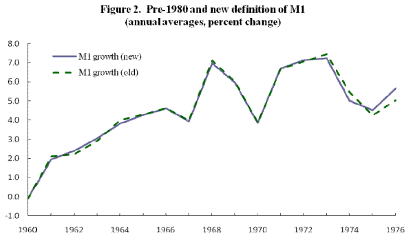
Some perspective on the behavior of monetary aggregates in the United States is provided by Figure 1, which plots quarterly observations on four-quarter growth rates of M1 and M2 since 1959. The modern M1 and M2 series were introduced by the Federal Reserve Board in 1980 (with some minor redefinitions thereafter). These series replaced narrower official definitions of each series.10 Despite their broader coverage, the pre-1980 growth rates of the modern definitions of M1 and M2 closely match those of the prior definitions. A partial demonstration of this fact is given in Figure 2, which plots growth in annual averages of the former M1 aggregate against the corresponding growth in the modern M1 series.11
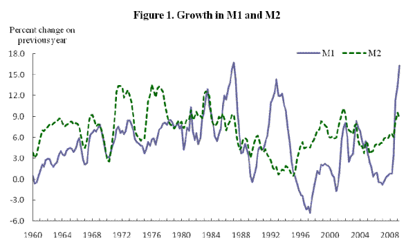
On the choice between M1 and M2 definitions, Friedman and Schwartz (1970, pp. 2, 92) stated: "important substantive conclusions seldom hinge on which definition is used... We have tried to check many of our results to see whether they depend critically on the specific definition used. Almost always, the answer is that they do not..."12 This conclusion has not proved to be durable. For much of the period since 1970, the M1 and M2 series have moved differently. Regulation Q was cited as a factor promoting discrepancies between M1 and M2 growth in the late 1960s and 1970s. But the abolition of Regulation Q did not bring an end to the discrepancies between M1 and M2 growth. On the contrary, the deregulated environment prevailing since the early 1980s seems to have perpetuated the differences in the behavior of the rates paid on M1 and M2 deposit balances. The result has been an intensification of the discrepancies between the growth rates of the M1 and M2 aggregates.
A change in interest paid on the deposits included in a monetary aggregate (and so a rise in the own-rate on money), holding constant the interest rates on securities, tends to change the real demand for that aggregate. Whether this affects the growth rate of the nominal quantity of money of depends on the operating procedure of the monetary authority. When the Federal Reserve uses an interest-rate instrument, it must acquiesce to the implications for money growth of its interest-rate choices. Consequently, the discrepancies between M1 growth and M2 growth in practice frequently reflect the different opportunity costs associated with the two aggregates.
Discussions of the effect of financial deregulation and innovation on the behavior of monetary aggregates often include the claim that the advent of payment of interest on M1 deposits has greatly changed the character of M1.13 While this argument appears to be important for the analysis of the international experience with deregulation,14 it has limited validity for the United States. The prohibition of interest on demand deposits has in fact never been lifted in the United States. The M1 series, as redefined in 1980, does include, in addition to currency and demand deposits, the category of other checkable deposits (OCDs), i.e., certain non-demand, checkable deposits that can legally bear interest. The OCD component of M1 rose relative to the demand deposit portion of M1 during most of the 1980s, suggesting that the interest return on OCDs had some attraction to bank customers. But, on the whole, it seems that explicit interest on M1 deposits has not proved to be a major factor affecting portfolio decisions. Convention, surviving regulations, and continuing differences in the transactions services provided by M1 funds compared to non-M1 M2, have all meant that the rate of return on M1 deposits has rarely been attractive relative to other deposit rates even in the era of deregulation.
The fall in M1 velocity in the 1980s has occasionally been attributed to the payment of interest on M1. But M1 velocity movements up to the late 1980s appear to be well captured by the declining opportunity cost of holding money as recorded in market interest rates, without recourse to an explanation that involves a changing own-rate on M1 (Lucas, 1988; Hoffman and Rasche, 1991; Stock and Watson, 1993).
Generally speaking, therefore, the whole of M1 is interest sensitive, and a rise in securities market interest rates promotes flows out of M1 balances. By contrast, from the late 1970s onward, the proportion of non-M1 M2 deposits bearing market-related interest rates rose considerably, standing at over 60% by early 1982 (Gramley, 1982). The overall interest sensitivity of M2 arises primarily from the fact that the rates on several classes of deposit, such as retail certificates of deposit, within M2 adjust to securities market interest rates only with a delay.
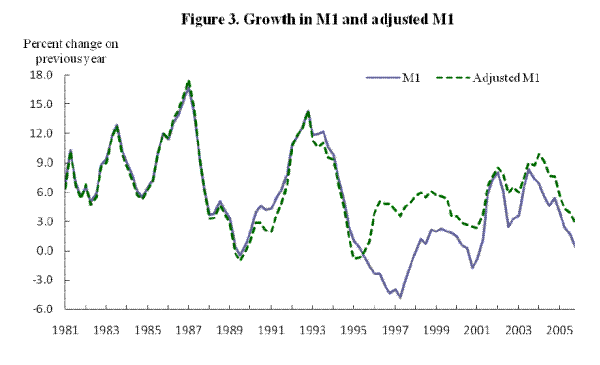
A different means through which financial innovation affects M1 behavior has proved to be much more significant in practice. "Sweeps" programs allow routine transfers, at the banks' initiative, between M1 deposits and non-M1 deposits. An embryonic version of this arrangement developed during the 1970s in the form of the automatic transfer system (ATS) (see Hafer, 1980), but extensive adoption of retail sweep deposit programs on the part of banks did not take effect until January 1994 (Anderson, 2003). The arrangement is attractive to depositors because of the better returns on non-M1 M2 deposits, and appeals to banks as a means of avoiding the more onerous reserve requirement on M1 deposits. The resulting portfolio behavior is believed to have created variations in M1 that have little macroeconomic meaning, with Anderson (2003, p. 1) arguing, "Retail-deposit sweep programs are only accounting changes: they do not affect the amounts of transaction deposits that banks' customers perceive themselves to own." (Italics in original.) A series of studies (including Jones, Dutkosky, and Elger, 2005, and Cynamon, Dutkowsky, and Jones, 2006) has attempted to correct the U.S. monetary aggregates for the effect of the sweep program. Figure 3 plots growth in M1 against growth in an adjusted M1 series. The deposits component of this adjusted series, following Ireland (2009), is based on replacing M1 deposits after 1993 with the Cynamon-Dutkowsky-Jones M1 deposit series that corrects for sweeps. In addition, the adjusted series used in Figure 3 excludes the Federal Reserve Board's estimates (available from 1964 onward) of U.S. currency held abroad, as reported in the flow of funds. We see from Figure 3 that these adjustments, on balance, lead to a more moderate decline in M1 growth during the late 1990s.
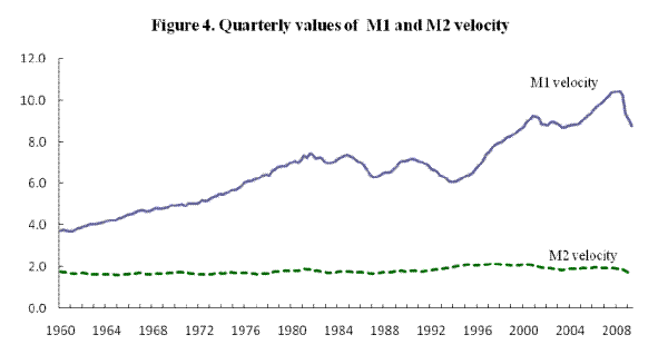
Figure 4 plots the velocities of M1 and M2. As is well known, the combination prevailing before the early 1980s was of an upward-trending M1 velocity and a stationary M2 velocity. As is also well known, M1 velocity underwent a major break in trend after 1981. (The apparent resumption of an upward M1 velocity trend in the late 1990s is largely illusory, reflecting the sweeps programs.) The presentation of both series on the same scale in Figure 4 means that M2 velocity appears very stable over the whole sample. But on closer inspection there are several notable shifts in the series--including a fall in M2 velocity with the introduction of money market deposit accounts in 1983 Q1, followed by a major velocity rise in the mid-1990s,15 and a decline, not fully reversed, that occurred during the monetary policy easing and international turmoil of 2001-2002.
One argument that has been advanced to explain the stability of M2 velocity is that the sweeps program itself tends to produce variations in M1 that cancel within M2. Beyond this more or less mechanical basis for favoring M2, it is also possible that M2 might be preferable even from the perspective of standard theories of money demand. While the M1 definition was intended to capture the concept of transactions balances, some of the non-M1 components of M2, such as money market deposit accounts, might be used routinely for performing transactions. In that case, the medium-of-exchange concept of money might better be represented by M2. Dorich (2009) argues that M2 should be used as the empirical measure of transactions money, and Reynard (2004) does so excluding one class of M2 deposit (namely, small time deposits, in recent years about one-seventh of M2). Arguing somewhat against the use of M2-type series as measures of transactions money, at least for studies using long sample periods, are the empirical results coming from the Divisia procedure, which Lucas (2000) argues is the best way to construct monetary aggregates. The Divisia procedure produces a series that downweights much of the non-M1 component of M2, and leads to quite different behavior of M2 and Divisia M2 during key episodes in the 1970s and 1980s (see Barnett and Chauvet, 2008).
5. Flawed evidence on money growth-inflation relations
A number of test procedures have been widely advanced as yielding evidence--pro or con--regarding quantity-theory relations between money growth and inflation. Two of the most prominent test procedures, however, are conceptually flawed. These are procedures based on: (i) determination of long-run money demand stability; (ii) regressions of inflation on money growth (or scatter plots of the series) using cross-country averages). We discuss each in turn.
5.1 Evidence on money demand stability
Quantity-theory relations between money growth and inflation do not depend on constancy of all parameters in an estimated money demand function, nor on cointegration among the components of the money demand function. To see this, let us write down a standard money demand equation:
| log ( |
(3) |
where ![]() and
and ![]() are positive. This is the typical specification (possibly with aggregate consumption
are positive. This is the typical specification (possibly with aggregate consumption ![]() substituting for aggregate output
substituting for aggregate output ![]() that would emerge from utility analysis (e.g., McCallum and Goodfriend, 1987; Lucas, 1988, 2000), other than our inclusion of the c
that would emerge from utility analysis (e.g., McCallum and Goodfriend, 1987; Lucas, 1988, 2000), other than our inclusion of the c![]() term. This linear trend term is designed to capture smooth progress in payments technology, which we will take as exogenous.16 If the financial system develops in a way that allows agents to economize on their money holdings over time, then
term. This linear trend term is designed to capture smooth progress in payments technology, which we will take as exogenous.16 If the financial system develops in a way that allows agents to economize on their money holdings over time, then ![]()
![]() 0. With a unitary income elasticity and a stationary nominal interest rate, the trend term implies a rising trend in velocity, i.e., real balances grow at a slower rate than real income.
0. With a unitary income elasticity and a stationary nominal interest rate, the trend term implies a rising trend in velocity, i.e., real balances grow at a slower rate than real income.
Money demand and cointegration studies are often motivated by the claim that money demand stability is a condition for the existence of quantity-theory relations between money growth and inflation. Lucas (1980), however, rejects the alleged dependence of a money growth/inflation link on money demand stability. There are several reasons to support Lucas' position. For example, a unit root in ![]() , the money demand shock in equation (3), would be considered a violation of dynamic stability in the money demand function, implying no cointegration and, by some definitions, money demand instability; but it would imply a first-difference relation,
, the money demand shock in equation (3), would be considered a violation of dynamic stability in the money demand function, implying no cointegration and, by some definitions, money demand instability; but it would imply a first-difference relation,
| (4) |
and hence a unitary money growth/inflation relationship, conditional on other variables. In particular, with stationary ![]() behavior,
behavior,
| E[ |
(5) |
so that there is on average a one-for-one relation between money growth, adjusted for output growth, and inflation. Hence, as argued by McCallum (1993), lack of cointegration between the levels of money (or money per unit of output) and prices is not a problematic result for the quantity theory.
Likewise, a change in the intercept term in the money demand function would permanently shift the relationship between the levels of money and prices, but would, once the shift to the new intercept was complete, wash out entirely from the first-differenced money demand function which is the underpinning of the money growth/inflation relationship. Furthermore, a one-time shift in the long-run interest semielasticity of money demand, such as has been argued by Ireland (2009) to have occurred in recent years in the case of M1 demand, does not affect the longer-term relation between money growth and inflation, provided ![]() averages zero. Summing up, while the price level homogeneity of the money demand function is crucial for delivering quantity-theory relations, instability in several other aspects of the long-run money demand relation does not preclude a close relation between money growth and inflation.
averages zero. Summing up, while the price level homogeneity of the money demand function is crucial for delivering quantity-theory relations, instability in several other aspects of the long-run money demand relation does not preclude a close relation between money growth and inflation.
It should furthermore be clear that, as Lucas (1980) also argued, money demand stability is consistent with a weak relationship between inflation and monetary growth. The case of M1 in the United States is perhaps the best example. As noted above, long-run M1 demand behavior up to the late 1980s appeared explicable via a standard demand function for money. But the M1 growth/inflation relationship seemed to break down in the early 1980s. The discrepancy between M1 growth rates and inflation is attributable to the sustained change in the opportunity cost of holding money. The ![]() term in equation (4) above, instead of averaging zero, was negative on average, and this declining opportunity cost of holding money promoted a recovery of real money balances. To be sure, a tendency toward nonzero
term in equation (4) above, instead of averaging zero, was negative on average, and this declining opportunity cost of holding money promoted a recovery of real money balances. To be sure, a tendency toward nonzero ![]() was not exceptional by postwar standards. The
was not exceptional by postwar standards. The ![]() term had been on average positive in the 1950s, 1960s, and 1970s. This led Barro (1982) to dispute the way that contributions of velocity growth to inflation were typically characterized in presentations of the quantity theory. These expositions tended to treat velocity growth arising from interest-rate increases as a "one-time" factor, affecting the price level but not the trend of prices. Barro pointed out that, with
term had been on average positive in the 1950s, 1960s, and 1970s. This led Barro (1982) to dispute the way that contributions of velocity growth to inflation were typically characterized in presentations of the quantity theory. These expositions tended to treat velocity growth arising from interest-rate increases as a "one-time" factor, affecting the price level but not the trend of prices. Barro pointed out that, with ![]() in practice trending upward, the contribution that velocity growth made to U.S. inflation, when measuring money with the M1 definition, turned out to be substantial. The contribution of
in practice trending upward, the contribution that velocity growth made to U.S. inflation, when measuring money with the M1 definition, turned out to be substantial. The contribution of ![]() to velocity growth over these decades was, however, steady enough that it did not prevent a close correlation between inflation and prior monetary growth. After 1981, the trend of
to velocity growth over these decades was, however, steady enough that it did not prevent a close correlation between inflation and prior monetary growth. After 1981, the trend of ![]() turned downward. But the actual decline in
turned downward. But the actual decline in ![]() , and associated fall in velocity, came in spurts. For example, the decline in the federal funds rate that took place in the second half of 1982 was almost entirely reversed in the course of the Federal Reserve's tightening over most of 1983 and 1984; but in 1985 and 1986, interest rates fell to levels not seen since the early 1970s. Thus, instead of the interest-rate decline contributing to a more or less constant difference between M1 growth and inflation, it affected M1 velocity growth markedly in specific periods, notably mid-1982 to mid-1983 and 1985-86, essentially wiping out the correlation between inflation and money growth once these periods were incorporated into calculations.
, and associated fall in velocity, came in spurts. For example, the decline in the federal funds rate that took place in the second half of 1982 was almost entirely reversed in the course of the Federal Reserve's tightening over most of 1983 and 1984; but in 1985 and 1986, interest rates fell to levels not seen since the early 1970s. Thus, instead of the interest-rate decline contributing to a more or less constant difference between M1 growth and inflation, it affected M1 velocity growth markedly in specific periods, notably mid-1982 to mid-1983 and 1985-86, essentially wiping out the correlation between inflation and money growth once these periods were incorporated into calculations.
The downward trend in nominal interest rates has continued in the 1990s and 2000s, with both the real interest rate and the expected-inflation component declining. While financial developments such as sweeps have undoubtedly contributed to distortions to both M1 growth and M1 demand, one should not expect a close money growth/inflation relation even in the absence of such distortions, because of the uneven but substantial shifts in the opportunity cost of holding money.
The fact that there is not a close mapping between stability of money demand and closeness of the money growth/inflation relationship provides the reason why we do not review studies of money demand in this paper. We do, however, discuss below the available evidence on the income elasticity of money demand, which does have bearing on the money growth/inflation relationship, and on the nominal homogeneity of money demand.
5.2 Evidence with country-average data
One popular way of scrutinizing putative quantity-theory relations is to construct per-country average observations on money growth and inflation, for use in scatter plots or in regressions (possibly with panel data) of inflation on money growth. When high double-digit inflation countries are included, scatter plots of annual averages of money growth and inflation tend to bring out an impressive relation (see, for example, Friedman, 1973, p. 18; Lucas, 1980, Figure 1; and McCandless and Weber, 1995, Chart 1). Results for countries which have experienced average inflation in single digits tend to be more mixed. For example, Issing, Gaspar, Angeloni, and Tristani (2001, p. 11) display, for a set of "low-inflation" countries, a scatter of mean money growth and inflation rates; they treat the quantity theory of money as implying a unitary slope for the plot, and fail to reject this slope restriction. De Grauwe and Polan (2005), on the other hand, find a poor relation between averages of money growth and inflation for low-inflation countries, although much stronger results have been reported in an exercise by Frain (2004) using the same sources for data as De Grauwe and Polan.
Favorable or unfavorable, these results using cross-country data are flawed as evidence on the quantity theory. A limiting case brings out the point. Consider two countries, ![]() and
and ![]() , in both of which there is no change in real income or nominal interest rates over time, and no money demand shocks. Then the first-differenced money demand equation implies that the money growth/inflation correlation is perfect in each country, i.e.,
, in both of which there is no change in real income or nominal interest rates over time, and no money demand shocks. Then the first-differenced money demand equation implies that the money growth/inflation correlation is perfect in each country, i.e., ![]() log
log ![]() log
log ![]() , for
, for ![]() ,
, ![]() . But the non-inflationary rate of money growth will not be identical across countries, except in the special case of identical trends in payment technology,
. But the non-inflationary rate of money growth will not be identical across countries, except in the special case of identical trends in payment technology, ![]() . The flaw in tests of the quantity theory based on cross-country averages is that they impose a constant
. The flaw in tests of the quantity theory based on cross-country averages is that they impose a constant ![]() value across each country--in essence, a common trend to velocity across countries.
value across each country--in essence, a common trend to velocity across countries.
Studies of money growth and inflation across countries have rarely recognized this point; an exception is Parkin (1980, p. 172), who correctly noted for six major countries that "there is virtually no association between averages of inflation and money growth," owing not to the absence of a within-country money growth/inflation link, but to "different trend changes in the demand for M1 balances arising from financial innovations." The point is of crucial quantitative significance when it comes to studying low-inflation countries. To take an example, Germany had lower inflation in the United States over 1962-79: 3.7% CPI inflation in Germany, 4.9% in the United States. But M1 growth over 1962-79 averaged 8.3% in Germany (with 4.6% growth in M1 per unit of output) and 5.3% in the United States (1.4% growth in per-unit terms). An approach that focused on these cross-country averages would suggest that inflation was not closely related to money growth. But, in each country, inflation was highly correlated with prior M1 growth over the 1962-79 period, with time series evidence supporting an approximately unitary relation. The cross-country approach neglects the different velocity trends across countries and fails to bring out the money growth/inflation relation that is obtainable from time series evidence.17
Admittedly, under very high inflation conditions, the trend in velocity due to exogenous improvements in payments technology is typically swamped by other factors: the inflation rates associated with rapid rates of money growth are large relative to the exogenous velocity trend.18 This accounts for the fact that money growth/inflation correlations computed from cross-country averages often look impressive despite the flaws inherent in this type of evidence.
6. Money growth and inflation in time series data
In this section we consider the time series relationship between money growth and inflation. Our contention is that while the static, contemporaneous relationship between monetary growth and inflation is weak, it is not the case that the only horizon at which the relationship becomes significant is at the very long run. Rather, inflation is strongly, though not at all perfectly, correlated with monetary growth of the immediately preceding years. This is the case whether one is considering quantitative experiments with standard models or drawing on evidence from historical time-series data.
In taking this position, we are challenging a view that has been widely expressed in the literature, both by critics and advocates of the use of money in monetary policy analysis. For example, while advocating the use of money in policy analysis, Assenmacher-Wesche and Gerlach (2007) do so subject to the qualifier (p. 535) that "money growth and inflation are closely tied only in the long run." That position could be taken as supportive of Svensson's (1999, p. 215) criticism that "this long-run correlation is irrelevant at the horizon relevant for monetary policy."
Svensson's claim that a very long-run relationship lacks any policy relevance seems doubtful, since policymakers are concerned with very long-term inflation expectations. But the more general notion that quantity-theory considerations only "bite" at very long horizons does seem to reduce the QTM's relevance for monetary policy decisions. In questioning this notion, it is useful to consider first the practice of taking long moving averages of data in studying the quantity theory, as we do in Section 6.1. Then we turn to the time-series relationship between money growth and inflation, both in quantitative models (Section 6.2) and in historical data (Sections 6.3 to 6.6). We finally consider evidence for the United States pertaining to the QTM's nominal homogeneity proposition (Section 6.7).
6.1 Is long averaging of data required?
We noted above that an implication of the QTM is that steady-state money growth rates and steady-state inflation rates are linked one-for-one, once allowance is made for output growth. Lucas (1980, 1986) argues that, in studying time series of a particular country, this steady-state relation can be brought out by taking long moving averages of monetary growth and inflation. Lucas (1986, p. S405) goes so far as to say, "Without such averaging, the quantity theory... does not provide a serviceable account of comovements in money and inflation." The argument that taking long moving averages of time series is the way to recover close money growth/inflation relations is also advanced in empirical studies such as Dewald (2003).
One objection to this procedure, which is not the criticism on which we focus here, is examined in detail by Sargent and Surico (2008). The interpretation of coefficient estimates in a regression of inflation (or its moving average) on a moving average of monetary growth will depend on whether past quarters' money growth rates (which enter the calculation of the moving average) are actually standing in for expectations of future money growth. If that is so, then the coefficient estimate associated with the average-money-growth term will not tend to 1.0 even in an environment where the quantity theory is valid; it will be a function of the policy rule parameters, for the same reason as that discussed in the literature on the natural rate hypothesis.
Sargent and Surico explore the behavior of the coefficient on the money growth term in moving-average regressions from simulations of a variety of models. Some of the models and parameter values contemplated do deliver large departures from a unitary money growth/inflation relation, and hence serve as one argument against the moving-average approach.19 But the practical relevance of their results for monetary policy models used in practice is open to question. Even under the conditions contemplated by Sargent and Surico, the coefficient on average money growth does tend to unity if long-term inflation is a unit root process, as it is assumed to be in Smets and Wouters (2007) and Woodford (2008), for example. Moreover, as detailed below, when we simulate a standard New Keynesian model with a standard interest-rate rule, the money growth/inflation relation is approximately unitary even when money growth and inflation are stationary.20
Our criticism of the moving-average procedure is somewhat different. Time averaging is advertised as a means of allowing for lags--especially by McCandless and Weber (1995)-- but in practice it may do so poorly. In particular, long averaging does not appear in practice to deliver any greater improvement in fit of the QTM than be obtained by retaining the non-averaged time series data.
To see this, consider the data Lucas (1980) used in studying the United States. He used second-quarter observations for M1 growth and CPI inflation for 1955-75. Using the modern vintage of CPI data and the Lothian-Cassese-Nowak (1983) data on old M1 (which are close to the data used by Lucas), and taking the four-quarter log differences for each second-quarter observation, we present three regressions in Table 1. The first regresses inflation on money growth for 1955-75. This was the relationship which Lucas characterized as loose and which motivated his use of moving averages. The second regression replaces the annual data with (overlapping) five-year averages of the data (the average for 1956-60 being the first observation, 1957-61 the second, etc., for a total of 16 observations). The third and fourth regressions return to the annual data (with sample periods 1955-75 and 1960-75, respectively), but instead of specifying inflation as a function of the current year's money growth, they regress inflation on money growth two years earlier.
Taking moving averages does have the effect of moving the coefficient on money growth from significantly below unity to above 0.80--and insignificantly different from unity. But so too does the procedure of retaining the annual data while replacing current money growth with lagged money growth. It is clear that the improvement in the performance of the QTM as one moves to heavily averaged data is no better than that delivered by a time series calculation that allows for an interval between movements in money growth and in inflation.
Table 1. M1 growth/ CPI inflation relationship using different degrees of time aggregation, United States, 1955-1975
| Dependent variable | Explanatory variable | Sample period | Coefficient on money growth term (Standard Errors are in parentheses) | R2 |
|---|---|---|---|---|
| Annual inflation | Annual money growth | 1955-1975 | 0.515 (0.236) |
0.200 |
| Five-year moving average of inflation | Five-year moving average of money growth | 1960-1975 | 0.832 (0.134) |
0.732 |
| Annual inflation | Annual money growth lagged two years | 1955-1975 | 0.809 (0.178) |
0.518 |
| Annual inflation | Annual money growth lagged two years | 1960-1975 | 0.829 (0.214) |
0.517 |
Note: The annual data underlying the regressions are for four-quarter growth rates of M1 and the CPI for the second quarter of the year.
We suggest that this result is not special to Lucas' example. On the contrary, the timing relationships between money growth, nominal income growth, and inflation mean that similar results are likely to show up using other sample periods and other countries. Replacing a regression of inflation on money growth with moving averages of the same series changes the right-hand-side variable from current money growth to an average of current, prior, and future money growth terms. But movements in money growth tend on average to lead movements in inflation--a regularity noted even in classic contributions on the quantity theory by Hume (1752) and Wicksell (1915/1935), and stressed in the monetarist literature, especially by Milton Friedman from 1970 onward (for example, Friedman, 1972, 1987). It is a regularity that continues to be found in studies using more recent data (see Batini and Nelson, 2001; Christiano and Fitzgerald, 2003; Leeper and Roush, 2003). In the terminology of spectral analysis, there is a phase shift in the relationship between monetary growth and inflation.
Superficially, time-averaging might seem to go in the right direction in allowing for this phase shift, as the averaging introduces prior money growth into the right-hand-side monetary term. But it is an inadequate approach if inflation regularly follows money growth. A regression of time-averaged inflation on time-averaged money growth still implies a relationship between inflation and money growth that is on average contemporaneous; future money growth rates enter the right-hand-side expression with the same weight as lagged rates.
Thus, taking long moving averages of time-series data seems an undesirable means of extracting the relationship between monetary growth and inflation. It is preferable to continue to use non-averaged time series data, and to allow for lags explicitly instead of implicitly.
What about the argument that long averages help remove measurement error? We have much sympathy with the view that there are substantial problems with the measurement of money, and have noted that these are likely to distort the relationship between monetary growth and inflation. But this is not, so far as we can see, a low-frequency vs. high-frequency data issue per se; it seems unrealistic to expect that measurement problems matter only for the cyclical relationship and wash out of the long-run relationship.
6.2 Money growth/inflation dynamics in a New Keynesian model
In our discussion of U.S. time series data on money growth and inflation, it may be instructive to consider the relationship between money growth and inflation that emerges from quantitative experiments with a structural model of a kind often used in monetary policy analysis. We deploy a New Keynesian model, appended by a money demand function. The New Keynesian model is standard, other than featuring date-t-1 calculations for the expectations terms that appear in the IS and Phillips curves. The use of lagged expectations in the spending and pricing relations follows Svensson and Woodford (2005), and yields a simplified version of the more elaborate representation of inertia that is specified in Rotemberg and Woodford (1997). Accordingly, in place of equation (2), the Phillips curve takes the form:
| (6) |
This Phillips curve arises from an environment where those firms changing prices in the current quarter (i.e., period ![]() make decisions on the basis of the prior quarter's (i.e., period t-1) information set.
make decisions on the basis of the prior quarter's (i.e., period t-1) information set.
The IS equation is:
| (7) |
Here ![]() 0, and
0, and ![]() is an IS shock. We retain the money demand function (4), so portfolio decisions are based on realized output and interest rates.
is an IS shock. We retain the money demand function (4), so portfolio decisions are based on realized output and interest rates.
To complete the model, we assume that monetary policy follows, up to a white noise shock, a Taylor (1993) rule with smoothing:
| Rt = ρRRt-1 + (1 - ρR)( |
(8) |
We set the parameters as follows: ![]() = 0.99,
= 0.99, ![]() = 0.024,
= 0.024, ![]() = 0.5,
= 0.5, ![]() = 0.8,
= 0.8, ![]() = 0.125,
= 0.125, ![]() = 1.5,
= 1.5, ![]() = 1,
= 1, ![]() = 0.21 The money demand interest semielasticity
= 0.21 The money demand interest semielasticity ![]() is kept to 4, corresponding to the value suggested for the business cycle frequency by King and Watson (1996). We assume that the nonpolicy shocks (IS, money demand, and natural output shocks) are AR(1) processes each with autoregressive parameter 0.95 and innovation standard deviation of 0.5%. The monetary policy shock is also treated as white noise, as noted above, with standard deviation 0.2%.
is kept to 4, corresponding to the value suggested for the business cycle frequency by King and Watson (1996). We assume that the nonpolicy shocks (IS, money demand, and natural output shocks) are AR(1) processes each with autoregressive parameter 0.95 and innovation standard deviation of 0.5%. The monetary policy shock is also treated as white noise, as noted above, with standard deviation 0.2%.
We solve the model and compute impulse responses. Figure 5 plots the responses to a unit monetary policy shock of money growth, inflation, nominal interest rates, and nominal income growth (![]() , defined as
, defined as ![]() . The monetary policy shock lowers the nominal interest rate and leads to an immediate rise in money growth. Because of the delays implied by the lagged-expectation terms, real
spending (not shown) and inflation react with a delay to interest-rate movements. Thus money growth leads inflation in the responses, even though the term that drives inflation (i.e., the sum of current and expected future output gaps) is wholly forward-looking.
. The monetary policy shock lowers the nominal interest rate and leads to an immediate rise in money growth. Because of the delays implied by the lagged-expectation terms, real
spending (not shown) and inflation react with a delay to interest-rate movements. Thus money growth leads inflation in the responses, even though the term that drives inflation (i.e., the sum of current and expected future output gaps) is wholly forward-looking.
Figure 6 plots the model response to a unit IS shock. Again, money growth reacts ahead of inflation.
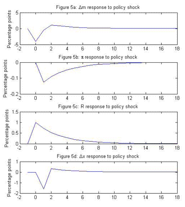
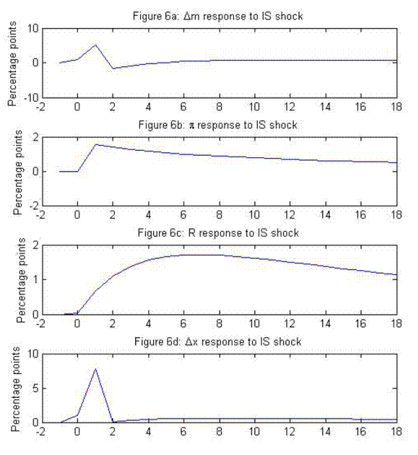
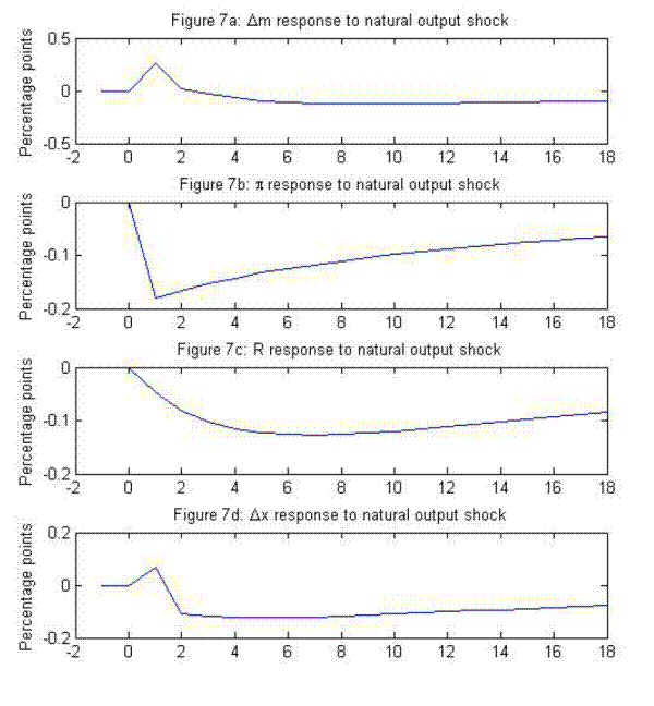
Figure 7 plots responses to a (positive) potential output shock. This shock reduces inflation after a one-period delay, while a policy loosening serves to brake the decline in inflation. The contemporaneous money growth/inflation relation is negative in this case, and the decline in inflation precedes an eventual decline in money growth. These patterns contrast with the lead of money growth over inflation observed in the previous responses. On the other hand, nominal income growth/inflation relation also differs from those previously depicted, as nominal income growth does not begin to decline until after the decline in inflation. This may suggest that the set of reactions associated with this shock is relatively unimportant empirically, since, as we discuss below, the average tendency in the data is for nominal income growth to lead inflation.
Four aspects of these results are worth cataloguing. First, money growth and inflation seem to be closely related--indeed, they seem to enjoy an approximately unitary relationship. This is despite the fact that the responses describe dynamics rather than steady-state relations. This standard New Keynesian model suggests that a great deal of the relationship between money growth and inflation is manifested at the business cycle frequency.
Second, money growth tends to have a contemporaneous or leading relation with inflation in this model. The Lucas (1980) approach to extracting quantity-theory relations can be thought of as implying a dependence of inflation on a two-sided distribution (i.e., both lags and leads) of money growth rates. The responses above suggest that in practice the future-money terms are less important for the study of the relation between inflation and money growth. This is despite the fact that, in the model, inflation is forward-looking when expressed in terms of the output gap. The decision delays built into the model confer on money a leading relationship. Also note that, in principle, following a shock that raises the level of money, the proportionality between money and prices can be restored by a return of the money stock to its original level; but that is not how the proportionality is principally restored for the shocks we consider. Rather, for IS and policy shocks, prices tend to move in the wake of the shift in money in a manner that restores the original level of real balances.
Third, the results with this model are not consistent with the notion that a policy rule that takes stabilizing actions against inflation is likely to have the effect of wiping out the money growth/inflation relation. The reasons this argument, which has appeared widely since the 1960s, does not appear relevant are, first, that the delays built into the model prevent complete stabilization of inflation, and, second, the inflation response coefficient of 1.5 implied by the Taylor rule still leaves some muted variation in inflation, which in turn has its counterpart in muted variation in monetary growth.
Fourth, while none of the responses depict the experiment we referred to in our definition of the QTM, i.e., an exogenous change in the money stock, they have several features common with the QTM experiment; the shocks contemplated in Figures 5 to 7 produce permanent changes in the levels of nominal money and prices, but only temporary movements in output and interest rates, and with the levels of money and prices restored to their original proportional relationship with one another.
These results reinforce the suggestion that quantity-theory relations should be recoverable from business-cycle data; that recovering the relation between inflation and money growth mainly involves looking at the relation between inflation and prior, not future, money growth; and that environments where policymakers follow a firm interest-rate rule tend to deliver traditional quantity-theory patterns in the reduced-form behavior of money and prices.
We consider the relationship further by computing a selection of second-moment statistics. Table 2 displays the correlations between inflation and (current and prior) monetary growth that emerge from simulations of the preceding model; specifically, the correlations tabulated are the averages of the correlations that arose from 100 simulated data series of 200 observations in length. The results indicate that money growth and inflation are positively correlated in the model with money growth leading inflation by a quarter.
We further report average coefficient estimates and R2 statistics that arise from regressions of inflation on money growth in the simulated data. A static regression delivers a coefficient on money growth of only 0.25. But when the regression specification includes lags of money growth, the coefficient sum rises to 0.93. Thus in this model the unitary relation between the two series, in principle visible completely only in the very long run, appears to be almost entirely recoverable from a reduced-form distributed -lag regression.
We have also considered an alternative New Keynesian model that replaces the Phillips curve with a curve based on indexation to lagged inflation. Equation (6) is replaced by:
| (8) |
Other than the dating of expectations to t-1, this specification follows Giannoni and Woodford (2002, eq. (2.1)), whose specification allowed for the dynamic indexation scheme advocated by Christiano, Eichenbaum, and Evans (2005). We assume partial indexation(i.e., ![]() = 0.2). The indexation feature, when combined with a stabilizing policy rule, tends to compress the variation of inflation. To compensate for this, we raise the output gap elasticity (
= 0.2). The indexation feature, when combined with a stabilizing policy rule, tends to compress the variation of inflation. To compensate for this, we raise the output gap elasticity (![]() to 0.15.
to 0.15.
Table 2a. Second-moment results, New Keynesian model:
Correlation of inflation and lag k of money growth
| k = 0 | k = 1 | k = 2 | k = 3 | k = 4 |
|---|---|---|---|---|
| 0.419 | 0.435 | 0.395 | 0.361 | 0.329 |
Table 2b. Second-moment results, New Keynesian model:
Regressions of inflation on money growth coefficient on lag of money growth
| 0 | 1 | 2 | 3 | 4 | 5 | 6 | Sum | R2 | |
|---|---|---|---|---|---|---|---|---|---|
| Static regression | 0.235 | --- | --- | --- | --- | --- | 0.235 | 0.167 | |
| Distributed-lag Regression | 0.166 | 0.179 | 0.169 | 0.149 | 0.121 | 0.089 | 0.062 | 0.935 | 0.579 |
Table 3a. Second-moment results, New Keynesian model with indexation:
Correlation of inflation and lag k of money growth
| k = 0 | k = 1 | k = 2 | k = 3 | k = 4 |
|---|---|---|---|---|
| 0.398 | 0.42 | 0.379 | 0.343 | 0.307 |
Note: All numbers reported in the tables are the averages across 100 stochastic simulations of output computed from time series of 250 generated data points.
Table 3b. Second-moment results, New Keynesian model with indexation:
Regressions of inflation on money growth coefficient on lag of money growth
| 0 | 1 | 2 | 3 | 4 | 5 | 6 | Sum | R2 | |
|---|---|---|---|---|---|---|---|---|---|
| Static regression | 0.318 | --- | --- | --- | --- | --- | 0.318 | 0.254 | |
| Distributed-lag regression | 0.241 | 0.205 | 0.187 | 0.154 | 0.117 | 0.075 | 0.042 | 1.022 | 0.593 |
Note: All numbers reported in the tables are the averages across 100 stochastic simulations of output computed from time series of 250 generated data points.
The second-moment results are given in Table 3. Here the correlation again is highest when money growth leads inflation, and the coefficient on money growth rises sharply when lags of money growth are included in regressions for inflation. The coefficient sum is here is very near to 1.0, so it is again the case that once allowance is made for lags, reduced-form regressions tend to convey the unitary relationship between money growth and inflation implied by the QTM.
Thus fortified by these model results, let us now examine the some examples of the empirical relation between money growth and inflation.
6.3 Nominal spending and inflation
Our contention that a relationship between money growth and inflation exists at the business cycle frequency does not rest on any claim that money appears in the structure of the IS or Phillips curves that describe spending and pricing decisions. Neither New Keynesian nor monetarist analyses imply the presence of money in the structural IS and Phillips curve equations, even though quantity-theory relations do prevail in models featuring these equations. The relationship in time series data between money growth and inflation rather is one that arises indirectly from the interaction of several equations. Indeed, since as Lucas (1986, p. S405) observes, "a change in money does not automatically cause prices to move equiproportionally in any direct sense," one important function of models of monetary policy analysis is to spell out the indirect process that tends to produce an equiproportionate relation between prices and money. This was seen in the preceding experiments with the New Keynesian model, where no money terms appeared in the system other than in the money demand relations, yet the model dynamics generated a close-to-unitary time series relationship between inflation and monetary growth.
In particular, the relationship between money growth and inflation is dependent on a relationship between nominal spending growth and inflation. Looseness in the relationship between monetary growth and nominal GDP growth will tend to imply a loose money growth/inflation relationship too. There is also a dynamic complication, for nominal spending growth tends empirically to exhibit timing relationships with its two components (real GDP growth and inflation) that should be taken into account when attempting to determine the money growth/inflation relationship. We state these two regularities before considering their implications for the study of monetary growth.
Nominal and real spending move together in the short run: In their study of U.S. monetary history, Friedman and Schwartz (1963, p. 678) observed that "real income tends to vary over the cycle in the same direction as money income does..." This observation holds true for U.S. data beyond the period covered by Friedman and Schwartz. McCallum (1988, p. 176) reports a correlation above 0.8 for 1954-85 quarterly changes in U.S. nominal and real GNP.22 Likewise, Brown and Darby (1985, p. 192) conclude from a study of annual data for several major countries that, contemporaneously, "the course of money income is much more closely related to that of real income than of price," while Woodford (2003, p. 188) notes "the persistence of the real effects of disturbances to nominal spending."
Inflation tends to follow nominal spending growth: The second regularity, consistent with but not implied by the first, is that inflation rates tend to be more closely related to prior nominal income growth than to same-period nominal income growth. This phenomenon was noted for the United States by Nelson (1978, p. 4) who stated, "An important conclusion is that the price level is very slow to respond to changes in nominal income."23 It is illustrated for several major countries in Table 4, which presents correlations of inflation with current and prior nominal GDP growth, for two inflation series (i.e., computed from the GDP deflator and the CPI), using annual data for selected sample periods.
The table documents a pronounced tendency for nominal income growth to have a better correlation with the following year's inflation than with current inflation. The lagged character of this relation is especially notable in the case of deflator inflation, a series which is biased toward having a close contemporaneous correlation with nominal GDP growth because of their connection via an identity.
Table 4. Correlations of inflation and nominal income growth
(Inflation in year t, nominal income growth in year t-k)
| GDP deflator inflation: k = 0 | GDP deflator inflation: k = 1 | CPI inflation: k = 0 | CPI inflation: k = 1 | ||
|---|---|---|---|---|---|
| Germany | 1957-1998 | 0.587 | 0.753 | 0.209 | 0.443 |
| Germany | 1980-1998 | 0.544 | 0.767 | 0.182 | 0.461 |
| Japan | 1959-2008 | 0.837 | 0.829 | 0.720 | 0.795 |
| Japan | 1980-2008 | 0.843 | 0.851 | 0.716 | 0.770 |
| United States | 1959-2008 | 0.624 | 0.708 | 0.541 | 0.709 |
| United States | 1980-2008 | 0.574 | 0.661 | 0.505 | 0.662 |
| United Kingdom | 1957-2008 | 0.923 | 0.834 | 0.893 | 0.845 |
| United Kingdom | 1980-2008 | 0.862 | 0.902 | 0.767 | 0.893 |
| United Kingdom | 1957-1972 | 0.785 | 0.860 | 0.761 | 0.808 |
| United Kingdom | 1977-2008 | 0.911 | 0.929 | 0.841 | 0.917 |
The full-sample correlations for the United Kingdom in Table 4 would appear to contradict the claim that nominal income growth leads inflation, but in fact do not do so. For most of the first quarter of 1974, the U.K. government imposed restrictions on days worked as an energy-conservation measure. As a result, recorded rates of both nominal and real U.K. GDP growth were artificially low in 1974, and nominal GDP growth did not peak until the inflation peak of 1975. Correlations for the United Kingdom omitting the mid-1970s observations reestablish a lead of nominal income growth over inflation, as the table shows.
6.4 Money growth per unit of output and inflation
What do these two regularities imply for the relationship between money growth and inflation? The principal implication is that, while money growth's correlation with inflation can be thought of as a by-product of the connection between monetary growth and nominal spending growth, money growth is likely to have different timing relations with the other two nominal aggregates.
With a unitary income elasticity, the demand for money function provides a connection of money to nominal income. As we have seen, the empirical relation between growth rates in nominal income and in prices seems to be close, but with nominal GDP growth tending to lead inflation. Taking these points together leads us to the implication that, when money growth is closely related to inflation, it is usually also closely related to nominal income growth. But different lags are relevant in each case; in annual data, money growth tends to be most closely related to current year's nominal income growth; but its maximum correlation with inflation is typically with inflation one or more years later. Consequently, there are problems with the procedure of adjusting money growth for output growth so as to obtain a measure of inflationary pressure. Over long periods, such an adjustment is appropriate, but over short periods, money growth adjusted for output growth may be an inferior indicator to money growth proper.
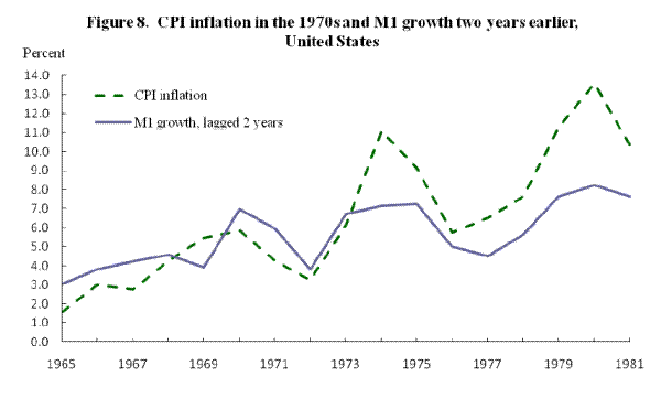
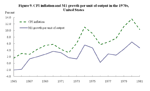
If correlations of money growth per unit of output growth and inflation are actually roundabout measures of the association between nominal income growth and monetary growth, they fail to capture the lead of money growth over inflation. That this is not simply a hypothetical issue is brought out by considering data for M1 growth and inflation in the United States in the 1960s and 1970s (Figures 8 and 9). The raw M1 growth data clearly lead movements in inflation; but adjusting for output growth delivers merely a contemporaneous money growth/inflation relationship.
Another problem inherent in comparisons of inflation with output-adjusted money growth is that the short-run nonneutrality of money may disguise the inflationary pressure implied by a given amount of money growth. In the late 1970s, for example, loose U.S. monetary policy led to rapid growth in both money and output. The strength of output disguised the longer-term weakness in output implied by the productivity slowdown, and indeed led some observers to contend that productivity from 1975 onward had returned to its pre-1973 rate of increase (see, for example, McNees, 1978, p. 56; Blinder, 1979, p. 67). Subtracting output growth from monetary growth in these years gave false comfort; the picture they conveyed suggested that policy settings were not as inflationary as they actually were.
6.5 Time series evidence
With this background, let us turn to reduced-form evidence on the relationship between money growth and inflation. We focus on annual data as they provide a convenient means of allowing for the possibility of lags between money growth and inflation of more than a year. We consider first the case of Japan, whose monetary experience illustrates several of the points noted above. Our data for Japan's M1 growth and CPI inflation are constructed from annual averages of data from International Financial Statistics. Regressions of inflation on money growth using this dataset are reported in Table 5.
We consider first the sample period 1959-1989. A static regression of inflation on money growth delivers an insignificant and low coefficient estimate. But this reflects not the absence of a relation in the time series data, but the failure to allow for lags; adding lags one to three of M1 growth to the specification has the effect of raising the R2 from 0.08 to 0.58. The sum of estimated coefficients on monetary growth is, however, only 0.44. The post- 1973 slowdown in Japan's real growth rate, which necessarily lowered the noninflationary rate of monetary growth, appears to be having a major impact on the results. Adding an intercept dummy equal to 1.0 after 1973 greatly improves the fit and interpretability of the regression, with the coefficient sum on money growth now 0.825 and insignificantly different from unity, and the coefficient on the dummy suggesting a rise in the inflation rate for given money growth (and a corresponding slowdown in potential growth, assuming a unit income elasticity of money demand) of 5.8%.
We also present results with money growth per unit of output as the explanatory variable. For the coefficient sum on money growth, the results that allow for lags closely agree with the results using M1 growth. The intercept dummy does not appear in the regressions because the per-unit term already adjusts for the slowdown in potential.
Results deteriorate when the sample period is 1959-2008. The post-1973 intercept dummy no longer seems to capture the growth slowdown well, and, while inclusion of lags of money growth raises the coefficient sum on money growth, the sum is still only 0.4. The results with per-unit money growth are poorer. The decade of the 1990s is not a decade in which the nonneutral effects of monetary policy average out; adjusting money growth for output growth worsens money growth as an indicator of inflation under these circumstances.
Do the full-sample results refute the quantity theory, or indicate a lack of practical usefulness in understanding inflation behavior? We would argue not. The collapse of nominal interest rates during the 1990s in Japan led to a series of permanent increases in real money demand that distorted the money growth/inflation correlation, as they did in the United States in the 1980s. From the viewpoint of the quantity theory, the trend in the opportunity cost of holding money in Japan during the 1990s illustrates a legitimate reason why there can be surges in money growth that never have a counterpart in inflation--particularly for a very interest-elastic aggregate like M1. That trend has left an indelible impression on the Japanese data, one that is unlikely to go away even with the taking of long averages. Nevertheless, an interest-rate trend is not something that can be confidently extrapolated. Once the economy has completely adjusted to a permanent decline in interest rates, the quantity theory suggests that the ceteris paribus unitary relation between money growth and inflation should become more evident.
Table 5a. Regressions for CPI Inflation in Japan (Sample Period: 1959-1989)
| Monetary Variable | Coefficients: Lag 0 | Coefficients: Lag 1 | Coefficients: Lag 2 | Coefficients: Lag 3 | Coefficients: Sum | Coefficients: D74 | R2 | SEE | DW |
|---|---|---|---|---|---|---|---|---|---|
| M1 growth | 0.178 | --- | --- | --- | 0.178 | --- | 0.082 | 0.040 | 0.840 |
| M1 growth standard errors | (0.110) | (0.110) | |||||||
| M1 growth | -0.279 | 0.214 | 0.311 | 0.196 | 0.441 | --- | 0.582 | 0.028 | 1.350 |
| M1 growth standard errors | (0.119) | (0.131) | (0.131) | (0.117) | (0.093) | ||||
| M1 growth | 0.067 | 0.278 | 0.313 | 0.166 | 0.825 | 0.058 | 0.735 | 0.023 | 1.460 |
| M1 growth standard errors | (0.133) | (0.108) | (0.107) | (0.095) | (0.126) | (0.015) | |||
| M1 growth per unit of output | 0.413 | --- | --- | --- | 0.413 | --- | 0.274 | 0.035 | 1.060 |
| M1 growth per unit of output standard errors | (0.125) | (0.125) | |||||||
| M1 growth per unit of output | 0.171 | 0.106 | 0.217 | 0.317 | 0.811 | --- | 0.639 | 0.026 | 1.480 |
| M1 growth per unit of output standard errors | (0.120) | (0.125) | (0.123) | (0.118) | (0.122) |
Note: A constant term was also included in all equations.
Table 5b. Regressions for CPI Inflation in Japan (Sample Period: 1959-2008)
| Monetary Variable | Coefficients: Lag 0 | Coefficients: Lag 1 | Coefficients: Lag 2 | Coefficients: Lag 3 | Coefficients: Sum | Coefficients: D74 | R2 | SEE | DW |
|---|---|---|---|---|---|---|---|---|---|
| M1 growth | 0.177 | --- | --- | --- | 0.177 | --- | 0.091 | 0.038 | 0.580 |
| M1 growth standard errors | (-0.081) | (-0.081) | |||||||
| M1 growth | -0.058 | 0.165 | 0.120 | 0.188 | 0.415 | --- | 0.365 | 0.033 | 0.660 |
| M1 growth standard errors | (-0.100) | (-0.122) | (-0.122) | (-0.101) | (-0.089) | ||||
| M1 growth | -0.061 | 0.164 | 0.119 | 0.187 | 0.409 | -0.001 | 0.365 | 0.034 | 0.670 |
| M1 growth standard errors | (-0.116) | (-0.124) | (-0.124) | (-0.103) | (-0.128) | (-0.015) | |||
| M1 growth per unit of output | 0.131 | --- | --- | --- | 0.131 | --- | 0.037 | 0.040 | 0.460 |
| M1 growth per unit of output standard errors | (-0.097) | (-0.097) | |||||||
| M1 growth per unit of output | 0.074 | 0.043 | 0.064 | 0.128 | 0.309 | --- | 0.108 | 0.039 | 0.450 |
| M1 growth per unit of output standard errors | (-0.120) | (-0.135) | (-0.134) | (-0.119) | (-0.135) |
Note: A constant term was also included in all equations.
Let us now consider the reduced-form relation between money growth and inflation in the United States. Table 6 presents regressions of inflation on money growth. Consider first the results with M1 as the measure of money. For the 1963-1979 sample, the coefficient sum on lags 0-3 of M1 growth is significant and very large. Indeed, it is well above unity. Allowing for the post-1973 growth slowdown via an intercept dummy brings the money-growth coefficient sum close to unity. But extending the sample period to 1989 destroys this result, making the sum negative. The 1963-89 regression result supports earlier evidence suggesting the breakdown of bivariate M1/inflation relations in the United States once observations from the 1980s are included in estimation (see, for example, Friedman and Kuttner, 1992). As noted previously, this deterioration reflected the protracted recovery of real M1 balances in response to permanent declines in U.S. nominal interest rates in the 1980s.
Adding the years 1990 to 2008 to the sample seems to restore some significance to M1 growth, but the coefficient sum is far below unity, and the explanatory power of the regression is low.
Moving to M1 growth per unit of output produces a near-unit sum on money growth for 1963-79. But it makes the money growth/inflation relation contemporaneous for the reasons discussed previously. There is a deterioration in the relation in the 1980s (not as great as the deterioration using M1 growth, because rapid output growth in 1983 and 1984 makes inflation in those years easier to reconcile with M1 behavior) and a further fall in the coefficient sum as 1990-2008 data are included.
The use of money per unit of output in the preceding regressions implicitly entailed an assumption of a unitary income elasticity of money demand; otherwise, it would not be appropriate to impose a unit weight on output growth in constructing a "money growth relative to output" series. For Japan, a unitary long-run elasticity of real M1 demand appears to have empirical support (Rasche, 1990), and many econometric studies for U.S. real M1 demand also support a unitary income elasticity (see Lucas, 1988; Hoffman and Rasche, 1991). There is some evidence, however, that the long-run income elasticity of M1 demand is better characterized empirically as 0.5 rather than 1.0 (see, for example, Ball, 2001). That being so, the "money growth relative to output" concept relevant for discussions of inflation should be measured as ![]() log(M1) - 0.5
log(M1) - 0.5 ![]() log
log ![]() rather than money growth per unit of output,
rather than money growth per unit of output, ![]() log(M1) -
log(M1) - ![]() log
log ![]() .
.
Table 6. Regressions for U.S. CPI inflation using M1
| Monetary Variable | Sample Period | Coefficients: Lag 0 | Coefficients: Lag 1 | Coefficients: Lag 2 | Coefficients: Lag 3 | Coefficients: Sum | Coefficients: D74 | R2 | SEE | DW |
|---|---|---|---|---|---|---|---|---|---|---|
| M1 growth | 1963-1979 | -0.085 | 0.624 | 0.995 | 0.214 | 1.748 | --- | 0.831 | 0.014 | 1.07 |
| M1 growth standard error | (-0.309) | (-0.336) | (-0.348) | (-0.270) | (-0.262) | |||||
| M1 growth | 1963-1979 | -0.103 | 0.507 | 0.877 | -0.037 | 1.244 | 0.026 | 0.947 | 0.008 | 2.20 |
| M1 growth standard error | (-0.180) | (-0.198) | (-0.204) | (-0.166) | (-0.184) | (-0.005) | ||||
| M1 growth | 1963-1989 | -0.271 | 0.044 | 0.003 | -0.136 | -0.359 | 0.038 | 0.278 | 0.029 | 0.42 |
| M1 growth standard error | (-0.287) | (-0.354) | (-0.397) | (-0.355) | (-0.435) | (-0.017) | ||||
| M1 growth | 1963-2008 | 0.094 | 0.021 | 0.127 | 0.143 | 0.384 | --- | 0.156 | 0.025 | 0.46 |
| M1 growth standard error | (-0.169) | (-0.246) | (-0.249) | (-0.169) | (-0.150) | |||||
| M1 growth | 1963-2008 | 0.097 | 0.015 | 0.136 | 0.120 | 0.368 | 0.007 | 0.169 | 0.026 | 0.44 |
| M1 growth standard error | (-0.170) | (-0.247) | (-0.251) | (-0.173) | (-0.151) | (-0.009) | ||||
| M1 growth relative to output: Δ log (M1/Y) | 1963-1979 | 0.925 | 0.030 | 0.065 | 0.125 | 1.145 | --- | 0.735 | 0.018 | 1.00 |
| M1 growth relative to output: Δ log (M1/Y) standard errors | (-0.264) | (-0.268) | (-0.255) | (-0.230) | (-0.210) | |||||
| M1 growth relative to output: Δ log (M1/Y) | 1963-1989 | 0.398 | -0.064 | 0.225 | -0.095 | 0.464 | --- | 0.184 | 0.03 | 0.59 |
| M1 growth relative to output: Δ log (M1/Y) standard errors | (-0.245) | (-0.282) | (-0.306) | (-0.259) | (-0.236) | |||||
| M1 growth relative to output: Δ log (M1/Y) | 1963-2008 | 0.273 | -0.087 | 0.109 | 0.080 | 0.376 | --- | 0.188 | 0.025 | 0.52 |
| M1 growth relative to output: Δ log (M1/Y) standard errors | (-0.139) | (-0.194) | (-0.195) | (-0.137) | (-0.127) | |||||
| M1 growth relative to output: Δ log (M1/Y0.5) | 1963-1979 | 0.925 | 0.294 | 0.474 | -0.161 | 1.532 | --- | 0.715 | 0.018 | 1.04 |
| M1 growth relative to output: Δ log (M1/Y0.5) standard errors | (-0.541) | (-0.548) | (-0.497) | (-0.445) | (-0.281) | |||||
| M1 growth relative to output: Δ log (M1/Y0.5) | 1963-1989 | 0.242 | -0.025 | 0.312 | -0.062 | 0.468 | --- | 0.108 | 0.031 | 0.50 |
| M1 growth relative to output: Δ log (M1/Y0.5) standard errors | (-0.353) | (-0.438) | (-0.516) | (-0.417) | (-0.290) | |||||
| M1 growth relative to output: Δ log (M1/Y0.5) | 1963-2008 | 0.234 | -0.095 | 0.155 | 0.105 | 0.399 | --- | 0.167 | 0.025 | 0.51 |
| M1 growth relative to output: Δ log (M1/Y0.5) standard errors | (-0.175) | (-0.268) | (-0.271) | 0.174 | (-0.141) |
Note: A constant term was included in all equations.
Table 7. Regressions for U.S. CPI inflation using M2
| Monetary Variable | Sample Period | Coefficients: Lag 0 | Coefficients: Lag 1 | Coefficients: Lag 2 | Coefficients: Lag 3 | Coefficients: Sum | Coefficients: D74 | R2 | SEE | DW |
|---|---|---|---|---|---|---|---|---|---|---|
| M2 growth | 1963-1979 | 0.119 | 0.193 | 0.550 | 0.680 | 1.543 | --- | 0.714 | 0.018 | 0.77 |
| M2 growth standard errors | (-0.235) | (-0.259) | (-0.269) | (-0.229) | (-0.363) | |||||
| M2 growth | 1963-1979 | -0.050 | 0.027 | 0.395 | 0.333 | 0.705 | 0.026 | 0.753 | 0.018 | 0.60 |
| M2 growth standard errors | (-0.263) | (-0.281) | (-0.287) | (-0.346) | (-0.731) | (-0.020) | ||||
| M2 growth | 1963-2008 | 0.006 | -0.053 | 0.206 | 0.522 | 0.682 | --- | 0.417 | 0.021 | 0.48 |
| M2 growth standard errors | (-0.185) | (-0.241) | (-0.239) | 0.181 | (-0.152) | |||||
| M2 growth | 1963-2008 | 0.060 | -0.050 | 0.240 | 0.474 | 0.723 | 0.012 | 0.449 | 0.021 | 0.51 |
| M2 growth standard errors | (-0.185) | (-0.237) | 0.237 | (-0.181) | (-0.152) | (-0.008) | ||||
| M2 growth relative to output: Δ log (M2/Y) | 1963-1979 | 0.340 | -0.208 | 0.324 | 0.651 | 1.107 | --- | 0.657 | 0.020 | 0.98 |
| M2 growth relative to output: Δ log (M2/Y) standard errors | (-0.229) | (-0.240) | (-0.249) | (-0.235) | (-0.263) | |||||
| M2 growth relative to output: Δ log (M2/Y) | 1963-2008 | 0.364 | -0.074 | 0.120 | 0.309 | 0.718 | --- | 0.387 | 0.022 | 0.740 |
| M2 growth relative to output: Δ log (M2/Y) standard errors | (-0.133) | (-0.153) | (-0.151) | (-0.133) | (-0.148) |
Note: A constant term was included in all equations.
Results imposing the alternative income elasticity of 0.5 appear as the final three regressions of Table 6. The results agree closely with those that used a unit weight on output growth, with similar equation standard errors and comparable performances across different sample periods. In addition, as before, the expression of money growth in relative-to-output terms makes the coefficient on current money the dominant term in the sum of coefficients.
In Table 7 we present regressions of CPI inflation on M2 growth. The results help explain why many researchers (such as Benati, 2009) prefer to use that aggregate in empirical studies rather than M1.24 In the regressions with a post-1973 intercept dummy, the coefficient sum on M2 growth changes little as the sample is extended from 1979 to 2008, and has 1.0 within its confidence interval throughout. Not all is well with the M2/inflation relation; for example, the regression standard error rises as the sample is extended, and residual serial correlation is substantial. But the greater resilience of the M2 results to the inclusion of more recent years' data supports two points stressed earlier: that a filter is not required to establish a relation between money growth and inflation,25 and that, while measurement problems with money are undoubtedly significant in practice, many of the discrepancies that arose between M1 growth and inflation, especially those prior to 1994, are attributable to the substantial interest sensitivity of M1 balances, rather than to measurement problems with M1.
6.6 Panel data evidence for the G7
We now consider panel data evidence, using annual observations on CPI inflation and monetary growth for the G7. In order to avoid some of the problems associated with the effect of disinflation on M1 behavior, the monetary series we use is an M2-type aggregate. The sample period is 1958-2008 for four of the seven economies; for those members of the G7 that are now part of the euro area (France, Italy, and Germany), we consider data only for the pre-euro period 1958-1998.
We present several estimated specifications in Table 8. In all cases these are panel regressions of inflation on money growth which impose common slopes across countries. We experiment however with cases where the intercept is allowed to vary across countries. The first regression in Table 8 is a static regression with a single intercept imposed. This delivers a coefficient of money growth of 0.387 which is highly significant but well below unity and the regression itself has only mild explanatory power. Introducing lags of monetary growth raises the coefficient sum to about 0.50. We argued above that it is not an implication of the quantity theory that the intercept term in panel regressions is constant across countries. In the remaining regressions, we therefore relax this restriction by moving to a fixed-effects specification. This change in specification does significantly reduce the equations' residual standard error, but seems initially to leave the slopes at their previous fairly low estimated values. But once we allow, as we did in our previous time-series regressions, for breaks in the intercept term after 1973 to take the secular decline in real GDP growth into account, the fixed-effects panel regressions exhibit much higher slope estimates than their single-intercept counterparts. For example, the regression including lags 0, 1, and 2 of money growth that and allowing for cross-country variation in intercepts with a break in intercepts in 1973, exhibits a coefficient sum of 0.692 and an R2 of 0.614, compared to values of 0.494 and 0.354, respectively, in the single-intercept case.
Table 8a. G7 panel regressions for CPI inflation: Single intercept
| 0 Lag of money growth used | 0-2a Lag of money growth used | |
|---|---|---|
| Coefficient on money growth | 0.614 | 0.494 |
| Coefficient on money growth standard error | (0.040) | (0.039) |
| R2 | 0.227 | 0.354 |
| SEE | 0.035 | 0.032 |
a. Estimate reported is coefficient sum.
Note: Observations in all regressions is 327. Data consist of annual observations for 1958-2008 (1958-1998 for France, Italy, and Germany).
Table 8b. G7 panel regressions for CPI inflation: Multiple intercepts with breaks in 1974
| 0 Lag of money growth used | 0-2a Lag of money growth used | |
|---|---|---|
| Coefficient on money growth | 0.377 | 0.509 |
| Coefficient on money growth standard error | (0.039) | (0.038) |
| R2 | 0.314 | 0.454 |
| SEE | 0.033 | 0.029 |
a. Estimate reported is coefficient sum.
Note: Observations in all regressions is 327. Data consist of annual observations for 1958-2008 (1958-1998 for France, Italy, and Germany).
Table 8c. G7 panel regressions for CPI inflation: Multiple intercepts
| 0 Lag of money growth used | 0-2a Lag of money growth used | |
|---|---|---|
| Coefficient on money growth | 0.514 | 0.692 |
| Coefficient on money growth standard error | (0.043) | (0.040) |
| R2 | 0.463 | 0.614 |
| SEE | 0.029 | 0.025 |
a. Estimate reported is coefficient sum.
Note: Observations in all regressions is 327. Data consist of annual observations for 1958-2008 (1958-1998 for France, Italy, and Germany).
Our stochastic simulations with the New Keynesian models indicated that, when the QTM holds, distributed-lag regressions of inflation on money growth tend to generate a coefficient on money growth close to unity, but perhaps somewhat lower than unity: in our simulation of the New Keynesian model, a coefficient sum of about 0.90. The empirical panel regression, on the other hand, delivers a coefficient sum of about 0.7. This is also close to the coefficient sum we obtained in similar specifications for estimated on U.S. time series data using M2. This perhaps suggests that empirical difficulties with finding a satisfactory measure of money, while not eliminating the relationship between money growth and inflation in the data, are responsible for reducing the coefficient on money growth in this type of time series regression by about 0.20 or 0.25.
6.7 Money demand nominal homogeneity
Our definition of the quantity theory does not associate the quantity theory closely with propositions about the money demand function. We have, however, insisted that zero degree homogeneity with respect to nominal variables is a property of money demand that is implied by the quantity theory--the demand is for real balances, in terms of real determinants.26 We now consider U.S. M1 and M2 demand further in this light.
The nominal homogeneity restriction implies ![]() = 0 in the relation:
= 0 in the relation:
![]() log VM
log VM
![]() OPP
OPP![]() ,
,
where VM![]() is velocity, defined as nominal GDP divided by nominal money, and OPP
is velocity, defined as nominal GDP divided by nominal money, and OPP![]() is the opportunity cost of the relevant aggregate. We measure OPP
is the opportunity cost of the relevant aggregate. We measure OPP![]() for M1 by the federal funds rate
(annual average) and OPP
for M1 by the federal funds rate
(annual average) and OPP![]() for M2 by the spread between the federal funds rate and the M2 own-rate.27 A money demand relation can be cast as a velocity relation (with no separate real income term) if the money demand function has a unitary income elasticity, a property often found for M2 demand and, as noted
above, also a common finding for M1. Note that this recasting of the relationship as a velocity relation means a change in sign when interpreting the coefficient on the interest rate: a negative money demand interest semielasticity implies a positive velocity interest semielasticity.
for M2 by the spread between the federal funds rate and the M2 own-rate.27 A money demand relation can be cast as a velocity relation (with no separate real income term) if the money demand function has a unitary income elasticity, a property often found for M2 demand and, as noted
above, also a common finding for M1. Note that this recasting of the relationship as a velocity relation means a change in sign when interpreting the coefficient on the interest rate: a negative money demand interest semielasticity implies a positive velocity interest semielasticity.
Given the definition of velocity, the natural price series to use in testing the nominal homogeneity restriction is the GDP deflator. For completeness, however, we also present results using CPI inflation. We express the relation in first differences rather than levels to allow for the likely presence of permanent money demand shocks, which produce nonstationarity in velocity and imply that levels of real money and real income are not cointegrated (see McCallum, 1993).
Because GDP deflator inflation and velocity growth have a definitional relation with one another, measurement errors in inflation may produce a correlation between inflation and velocity growth. These errors would tend to bias tests in the direction of rejecting nominal homogeneity. To protect against this bias, we estimate by instrumental variables, with two lags of each series (velocity growth, inflation, and first difference of opportunity cost) serving as instruments.
Table 9. Tests of nominal homogeneity of M1 demand where the dependent variable is the log-difference in M1 velocity
| Sample period | Coefficients on GDP deflator (standard errors in parentheses) | Coefficients on CPI (standard errors in parentheses) | Coefficients on ΔOPP (standard errors in parentheses) | Coefficients on Δlog Yt (standard errors in parentheses) | SEE | DW |
|---|---|---|---|---|---|---|
| 1962-2008 | -0.010 (0.240) |
--- | 0.505 (0.535) |
--- | 0.034 | 0.76 |
| 1962-1993 | 0.301 (0.260) |
--- | 0.520 (0.543) |
--- | 0.032 | 0.73 |
| 1980-2008 | -0.344 (0.401) |
--- | 1.427 (0.745) |
--- | 0.037 | 0.77 |
| 1962-2008 | --- | 0.016 (0.209) |
0.595 (0.519) |
--- | 0.034 | 0.76 |
| 1962-1993 | --- | 0.199 (0.221) |
0.574 (0.536) |
--- | 0.032 | 0.73 |
| 1980-2008 | --- | -0.224 (0.352) |
1.339 (0.672) |
--- | 0.037 | 0.75 |
| 1962-2008 | -0.152 (0.329) |
--- | 0.498 (0.556) |
-0.328 (0.475) |
0.037 | 0.82 |
| 1962-1993 | 0.497 (0.376) |
--- | 0.306 (0.672) |
0.318 (0.462) |
0.031 | 0.70 |
| 1962-2008 | --- | -0.162 (0.328) |
0.612 (0.576) |
-0.386 (0.534) |
0.036 | 0.82 |
| 1962-1993 | --- | 0.399 (0.381) |
0.246 (0.567) |
0.361 (0.554) |
0.031 | 0.68 |
Note: Instrumental variables estimates are reported in the tables. Instruments are a constant and two lags of each variable, including dependent variable. "GDP deflator" and "CPI" refer to log differences of these variables.
Estimates, using annual data, are presented in Table 9 for M1 and in Table 10 for M2. We consider the full sample (starting in 1962 for the M1 velocity estimation, a year later for M2), and results for samples starting in 1980. Because of the increased importance of sweeps for M1 behavior after 1993, we also present results for the 1962-1993 in the case of M1 velocity.
Observing the point estimates and standard errors for ![]() , we see that nominal homogeneity of money demand is not rejected irrespective of the inflation series used, the definition of money chosen, or sample period considered. As the final rows in each table show, this continues to be the case if we relax the assumption of a unitary income elasticity of money demand.28 Thus, nominal homogeneity of money demand, a fundamental aspect of the quantity theory, appears to be consistent with the U.S. data.
, we see that nominal homogeneity of money demand is not rejected irrespective of the inflation series used, the definition of money chosen, or sample period considered. As the final rows in each table show, this continues to be the case if we relax the assumption of a unitary income elasticity of money demand.28 Thus, nominal homogeneity of money demand, a fundamental aspect of the quantity theory, appears to be consistent with the U.S. data.
Table 10. Tests of nominal homogeneity of M2 demand:
Dependent variable: Log-difference in M2 velocity
| Sample period | Coefficients on: GDP deflator (standard errors in parentheses) | Coefficients on: CPI (standard errors in parentheses) | Coefficients on: ΔOPP (standard errors in parentheses) | Coefficients on: Δlog Yt (standard errors in parentheses) | SEE | DW |
|---|---|---|---|---|---|---|
| 1963-2008 | 0.130 (0.147) |
--- | 0.634 (0.372) |
--- | 0.021 | 1.23 |
| 1980-2008 | -0.006 (0.237) |
--- | 1.076 (0.860) |
--- | 0.025 | 0.96 |
| 1963-2008 | --- | 0.172 (0.125) |
0.732 (0.360) |
--- | 0.020 | 1.24 |
| 1980-2008 | --- | 0.036 (0.179) |
1.394 (0.653) |
--- | 0.020 | 0.87 |
| 1963-2008 | 0.048 (0.193) |
--- | 0.740 (0.421) |
-0.290 (0.290) |
0.023 | 1.39 |
| 1963-2008 | --- | 0.049 (0.185) |
0.802 (0.437) |
-0.299 (0.320) |
0.022 | 1.40 |
Note: Instrumental variables estimates are reported in the tables. Instruments are a constant and two lags of each variable, including dependent variable. "GDP deflator" and "CPI" refer to log differences of these variables.
7. Implications of a diminishing role for money
Benjamin Friedman (1999, 2000) has suggested that technological improvement in the financial sector raises the prospect of the virtual obsolescence of central bank money. In terms of the subject matter of this paper, the scenario that Friedman envisages is consistent with continuing quantity-theory relations between inflation and money growth, provided that the latter refers to growth in deposit-inclusive measures of money. But both deposit creation and market interest rates would become disconnected, in this scenario, from central bank actions, with associated loss of central bank control over nominal spending.29 Friedman's argument does not involve the complete disappearance of money, but instead a state of affairs in which the role of base money diminishes to the point where central banks' ability to influence aggregate demand in a dependable fashion would be in jeopardy. Reactions to these conjectures include those of Goodhart (2000) and Woodford (2000, 2001). In the following paragraphs we attempt to outline the main contours, and evaluate the merits, of the debate.
Base money includes, of course, both currency and bank reserves. Goodhart (2000) argues convincingly that private sector demand for currency will persevere for the foreseeable future, in part because of the anonymity conferred on currency transactions. In principle, the interest elasticity of currency demand gives central banks scope to manipulate interest rates without departing from its traditional policy of providing the amount of currency that the public demands at prevailing income and interest rates. But this would constitute a departure from the standard central bank practice of focusing on interbank transactions as the means through which to affect interest rates.
One part of Friedman's (2000) argument is that technological progress makes it possible for buyers to make payments through accounts--bank or nonbank--that are not subject to reserve requirements. The existence of such arrangements is widely accepted by all participants in the debate. Woodford (2000) argues convincingly that the magnitude of required reserves is irrelevant. After all, several central banks do not rely on reserve requirements in their arrangements for setting interest rates. Overnight interest rates in these economies are typically controlled by means of "channel" arrangements, involving standing facilities that set both a floor and a ceiling on overnight rates. These rates apply to the operational reserve balances, useful for settlement purposes, which financial intermediaries hold with the central bank. An arrangement consistent with the channel system involves central bank payment of interest on reserves, including excess reserves; this possibility is discussed by Woodford (2000, 2001) and Goodfriend (2002). The arrangement offers the promise of securing a positive demand for central bank money in a technologically advanced financial system. If settlement reserves with the central bank are held by banks, along with overnight securities, then the interest rate on the latter will equal the sum of the interest rate paid on reserve balances plus the marginal service yield provided by these balances. By adjusting the interest paid on reserves, the central bank can exert a dominant influence on the overnight interest rate. The Federal Reserve introduced interest payments on reserves in October 2008.
One element of Woodford's optimistic discussion of the prospects for monetary policy in an economy with a negligible medium of exchange should be read with special care. That part includes his statement that "the unit of account in a purely fiat system is defined in terms of the liabilities of the central bank" (Woodford, 2000, p. 257). His subsequent discussion pertains to the unit of account (UOA) as so defined. But in many analyses the UOA is defined instead as the unit in which prices are quoted in most transactions; see, for example, Niehans (1978, pp. 118-119) and Jevons (1875, p. 5).30 Now certainly the liabilities of the central bank would be a favored candidate for the role of UOA under this second meaning for an economy with no medium of exchange (MOE), but there is no necessity that it be the one that prevails. Goods prices will, in a market economy, be quoted in terms of the medium that market participants find most convenient. Just as central bank currency can be supplanted by some other candidate medium of exchange if its supply is managed too badly (e.g., under hyperinflation conditions), the central bank's contender for the MOA can conceivably lose out to another medium. And it is the UOA in terms of the MOA actually prevailing in market transactions that is of macroeconomic importance; it is stickiness of those prices used in actual transactions that is relevant for the definition of real rates of interest that influence aggregate demand. Woodford (2000, pp. 257-258) understands this point--indeed, makes it explicitly himself. But the tone of his discussion is, we suggest, made considerably more optimistic (in the sense at hand) in its impression by his choice of definition.
8. Money vs. interest rates in price level analysis
The diminishing role for money provides a natural point of departure for a discussion of recent approaches to the analysis of price level determination and monetary policy operating procedures. The trend of professional work in recent years can be put in context by juxtaposing two observations from earlier decades: Patinkin's (1972, p. 898) statement that "one of the primary tasks of monetary theory is indeed to explain the determination of the wage and price levels," and Gowland's (1991, p. 122) observation that "the term `monetary policy' seems inappropriate in a model without money." The recent literature can be thought of as embracing the first observation while rejecting the second. Monetary policy analysis remains concerned with explaining price-level determination, but it has become prevalent in the course of such explanations to omit reference to monetary aggregates. In particular, the "cashless" and "neo-Wicksellian" treatment in Woodford (2003) represents a crystallization of a framework in which the central bank manipulates interest rates and in which there may be no medium of exchange, with price level variations nevertheless capable of being influenced by deviations of the real interest rate from the natural rate of interest.
8.1 Conditions for excluding money from the analysis
The result that no reference to money arises when working out inflation behavior is not special to the analysis of cashless economies. It holds whenever the money stock appears in the money demand equation but not in the IS or spending equations, monetary policy rule, or Phillips curve. In New Keynesian models that feature a transactions technology or money in the utility function, there are two principal requirements for obtaining solution expressions for inflation and the output gap does not require considering money stock behavior. These conditions are (i) the assumed monetary policy rule that do not feature a response to money (real or nominal) or monetary growth and (ii) the utility or transaction cost function is separable across money and consumption.
The exclusion of money from the IS and Phillips curves, in turn, is not special to New Keynesian analysis; on the contrary, it was typical in prior monetary analysis. In that earlier analysis, it was usually also the case that monetary policy effects on spending were specified as working through interest rates, making it possible, when studying interest-rate rules, to treat the system excluding money as self-contained, the money demand equation then standing alone, with money becoming a "residual" variable.31
What is different in the modern literature is that the cases where money can be neglected have been formalized as the two conditions given above, and these conditions appear to have become accepted as realistic assumptions for policy analysis and empirical work. To a far greater extent than previously, the literature has focused on interest-rate or targeting rules in which money does not appear. Moreover, a number of studies have argued that utility can be treated as approximately separable across money and other variables.32
The limiting case of no medium of exchange would, in our terms, indeed be a nonmonetary economy; there would be no monetary policy, literally defined. Nevertheless, as discussed above, there would be scope for different types of policy measures regarding price level behavior, with the price level being regarded as some general index of prices in terms of the unit of account.
If we do not adopt a literally cashless model--so that a positive demand for money exists--but we absorb the message that the separable-utility case as realistic, is there a useful role left for money in monetary policy formation? Or is it satisfactory to have interest rates as the sole monetary policy variable in the analysis?
In answering these questions, one should note that the shift toward analyses that ignore or downplay money largely reflects a change in empirical judgments. In the era in which monetary aggregates were used as guides to policy, policymakers expressed the view that--although monetary policy actions did work on spending via interest rates, and the authorities did typically employ a short-term nominal interest rate as their policy instrument--it was a more straightforward matter to establish money/inflation relations than it was to establish connections between policy-rate actions and subsequent inflation movements. For example, the Reserve Bank of New Zealand (1985, p. 627) stated that the "empirical linkages between interest rates and inflation are less well established than the linkages between monetary growth and inflation." Similarly, Federal Reserve Governor Henry Wallich (1985, p. 40) argued that the "impact on inflation of a given level of interest rates, nominal or real... is far less predictable" than the relationship between inflation and prior monetary growth.
These statements can be interpreted as reflecting doubts about the reliability of empirical estimates of the natural rate of interest. At any point, there is an actual level of the real short-term interest rate and there exists a natural value of that rate which by definition is consistent with price stability.33 Likewise, at any time there will be an observed rate of monetary growth and there will be a noninflationary growth rate of money corresponding to the rate at which money would grow if the real short-term interest rate were at its natural level. Predominant reliance on monetary-aggregate data in policymaking in these circumstances could reflect a judgment that estimates of the noninflationary rate of monetary growth are more reliable than estimates of the natural rate of interest. Conversely, the shift in recent decades toward policy frameworks that relied less on monetary aggregate data likely reflects a judgment that estimates of the natural rate of interest are more reliable than estimates of the noninflationary rate of monetary growth.
Interest in a Wicksellian approach to price-level analysis showed some signs of reviving at a policy level in the early 1990s (for example, Kohn, 1990), but has exploded in recent years in light of Woodford's (2003) emphasis on the role of the natural rate of interest in dynamic stochastic general equilibrium models. We have not contrasted Wicksellian and quantity-theory approaches up to this point because, provided that a medium of exchange is present, the two are compatible, being in essence alternative ways of viewing the same process, as is acknowledged by Woodford (2003, p.53).34 Wicksell (1915/1935), one might note, emphasized the money stock adjustments that were implied by the banking system's variations in interest rates, although he also considered a "pure credit" economy. And in dynamic general equilibrium models, the money demand function that implies a connection between steady-state money growth and inflation comes from the same private sector optimization that delivers the IS and Phillips curves that Woodford uses.
To facilitate the discussion, consider the following variant of the model of Section 6, written now without the Et-1 operators in the IS and Phillips curve relations, and including a Phillips curve shock term, so as to conform even more closely to the mainstream model of recent years:
| b1 < 0 | (9) |
| 0 > |
(10) |
| R |
μ1 > 1, |
(11) |
Here ![]() is log output,
is log output, ![]() is inflation,
is inflation, ![]() is the flexible-price (natural- rate) value of
is the flexible-price (natural- rate) value of ![]() , and
, and ![]() is the one-period interest rate controlled by the central bank.35
is the one-period interest rate controlled by the central bank.35
The basic point relating to the interest-rate policy rule is, as is very well known, that with ![]() taken for simplicity as exogenous, this system is complete, i.e., it suffices to determine values of the system's endogenous variables
taken for simplicity as exogenous, this system is complete, i.e., it suffices to determine values of the system's endogenous variables ![]() ,
, ![]() , and
, and
![]() . Consequently, if the economy includes medium-of-exchange money with a demand function of the form
. Consequently, if the economy includes medium-of-exchange money with a demand function of the form
| (12) |
with ![]() being the log of nominal money balances, the latter serves only to describe how much (high-powered) money needs to be supplied by the central bank in order to implement its policy rule (11). Thus a shift in the parameters of (12) would, if there were no change in the other structural equations (9)-(11), have no effect on the behavior of the key variables
being the log of nominal money balances, the latter serves only to describe how much (high-powered) money needs to be supplied by the central bank in order to implement its policy rule (11). Thus a shift in the parameters of (12) would, if there were no change in the other structural equations (9)-(11), have no effect on the behavior of the key variables ![]() ,
, ![]() , and
, and ![]() . It is true that the crucial absence from (9) of any term involving
. It is true that the crucial absence from (9) of any term involving ![]() depends upon the assumption of separability of the relevant underlying function describing the way in which money facilitates transactions. But, as noted above, analyses by Woodford (2003, pp. 111-123), McCallum (2000a, 2001), and Ireland (2004) indicate that taking account of a plausible degree of nonseparability would have a negligible effect on the behavior of the key variables. Consequently, the omission of money from policy analysis involving the standard model is not a prima facie reason to doubt the validity of studies that incorporate such an omission.36
depends upon the assumption of separability of the relevant underlying function describing the way in which money facilitates transactions. But, as noted above, analyses by Woodford (2003, pp. 111-123), McCallum (2000a, 2001), and Ireland (2004) indicate that taking account of a plausible degree of nonseparability would have a negligible effect on the behavior of the key variables. Consequently, the omission of money from policy analysis involving the standard model is not a prima facie reason to doubt the validity of studies that incorporate such an omission.36
8.2 Determinacy and learnability
Recently, however, a major challenge to the validity of the current mainstream approach has been put forth by Cochrane (2007), who strongly questions its basic economic logic, arguing that one standard presumption--namely that "determinacy" of a rational expectations (RE) equilibrium suffices to imply that stable inflation behavior will be generated when the Taylor principle is satisfied--is incorrect. His point is that New Keynesian models such as that expressed in (9)-(11) are typically consistent with the existence of RE paths with explosive inflation rates (in addition to one or more stable paths) that normally do not imply explosions in real variables relevant for transversality conditions. Consequently, the usual logic does not imply the absence of explosive inflation. This point is, we believe, correct--but it does not (we contend) justify Cochrane's negative conclusions about New Keynesian analysis. As argued in McCallum (2009), there is a different criterion that is logically satisfactory for the purpose at hand. This is the requirement that, to be plausible, a RE solution should satisfy the property of least-squares learnability of the type featured in the work of Evans and Honkapohja (2001). Adoption of this criterion amounts to a requirement of feasibility, with respect to available information, of a candidate equilibrium and accordingly should be attractive to analysts concerned with actual monetary policy. In the class of New Keynesian models discussed by Cochrane, it transpires that the learnability criterion singles out the standard New Keynesian solution as the only plausible equilibrium. In this respect, it serves to justify in principle a large portion of current mainstream monetary analysis.37
We now argue, nevertheless, that there is one respect in which a money stock growth rule is distinctly preferable to an interest rate rule, at least when analyzed in the context of a typical linear model that includes a standard money demand function.38 In particular, it is the case that for non-activist rules a money-growth rule (i.e., a constant money growth rate) with standard parameterization leads to a unique and stable RE equilibrium that is learnable--in the least-squares sense researched extensively by Evans and Honkapohja (2001)--whereas a constant interest rate rule does not give rise to any learnable RE equilibrium. The latter fact is fairly well known from writings by Woodford (2003, pp. 264-268), Bullard and Mitra (2002), and others. To demonstrate that a well-behaved RE equilibrium is, by contrast, learnable with a non-activist money growth rule, we proceed as follows.
Consider the standard linearized New-Keynesian model of equations (9)-(11) but in which there is, for simplicity, full price flexibility so that in each period output equals its flexible-price, natural-rate value
![]() . We measure all real variables as deviations from their natural-rate values so
. We measure all real variables as deviations from their natural-rate values so ![]() = 0 for all
= 0 for all ![]() and, after substituting in the identity
and, after substituting in the identity ![]() - pt-1, the model can be written as
- pt-1, the model can be written as
| 0 = 0 - |
(9') |
| (13) |
together with money demand equation (12). Equation (13) is the money supply rule. Then substitution of (12) into (9') yields
| 0 = |
(14) |
Inserting the money supply rule (13) and rearranging we then obtain
| (15) |
where k is a constant, and ![]() /(1 +
/(1 + ![]() satisfies the inequalities 0
satisfies the inequalities 0 ![]() 1. Here both mt-1 and
1. Here both mt-1 and ![]() are exogenous so the system has a single non-explosive solution that is learnable.39 Thus a non-activist money growth rule leads to a well-behaved RE equilibrium in which the inflation rate equals the money growth rate minus a term reflecting technical progress (which equals zero in the example above).40
are exogenous so the system has a single non-explosive solution that is learnable.39 Thus a non-activist money growth rule leads to a well-behaved RE equilibrium in which the inflation rate equals the money growth rate minus a term reflecting technical progress (which equals zero in the example above).40
To this argument it might be objected that for practical purposes it is the monetary base that the central bank can actually control, whereas the medium-of-exchange aggregate is what appears in the money demand equation in our model. That is true, so our analysis should also include a random component reflecting the semi-technological relationship between the two. But ignoring this distinction in our analysis is analogous to our treatment of interest rates in which we ignore the difference between the overnight interest rate typically controlled by a central bank and the longer-maturity market rates that are relevant for aggregate demand.
8.3 Fiscal theory of the price level
Probably the most drastic conceptual challenge to today's mainstream analysis, and also to traditional views concerning the relationship between money growth and inflation, has come not from empirical findings or the foregoing arguments, but from an intricate, elusive, and controversial doctrine known as the "fiscal theory of the price level" (FTPL), which was developed primarily by Leeper (1991), Sims (1994), Woodford (1994, 1995), and Cochrane (1998). We have not attempted to survey this topic in general because it is covered extensively in this volume of the Handbook by Canzoneri, Cumby, and Diba (CCD). We find admirable, in most respects, their excellent and thorough treatment. We believe, nevertheless, that ultimate disagreements concerning the FTPL result basically from differing strategies for responding to multiplicities of rational expectations solutions, as suggested in McCallum (1999).41 The most satisfactory means of dealing with such multiplicities seems to be, once again, provided by analysis of the learnability of the various solutions, following procedures of the type developed and exposited most prominently in the treatise of Evans and Honkapohja (2001). To date the most extensive application of these techniques to the FTPL is that of Evans and Honkapohja (2007). We have discussed these results at some length in McCallum and Nelson (2005), which concludes that (i) several of the phenomena implied by the FTPL are actually consistent with traditional monetarist doctrine42 and that (ii) our study's main messages for policy are that "central banks can control inflation irrespective of fiscal policy and that detailed coordination between monetary and fiscal authorities is not needed for effective macroeconomic policy" (2005, p. 581). The second of these conclusions, which we continue to support, constitutes a partial disagreement with the CCD emphasis on the necessity of monetary-fiscal coordination.
8.4 Money as an information variable
We have argued above that from a purely theoretical perspective it has become very widely
understood that analysis that posits an interest rate instrument and ignores monetary aggregates is coherent under the assumption that any absence of separability in the transaction-cost function that expresses the MOE (i.e., transaction facilitating) role of money43 is mild enough to be of negligible effect. That does not, of course, settle the issue of whether an interest rate or monetary aggregate rule would perform more satisfactorily in practice--or whether it is desirable for a central bank with an interest rate instrument to ignore entirely monetary aggregates. In this regard it deserves mention that Woodford (2008) has recently developed the "OK to ignore" position in considerable detail, arguing that several claims by others for the usefulness of monetary aggregates are actually based on the behavior of credit (rather than monetary) aggregates.
A different approach to this issue is developed in McCallum (2000b), which employs counterfactual historical comparisons of the type utilized by Stuart (1996) and Taylor (1999). This type of analysis proceeds by contrasting actual settings of potential instrument variables during important historical time spans with the values that would have been specified by particular rules in response to prevailing conditions. Discrepancies between rule-specified and actual values are then evaluated, in light of ex post judgements concerning macroeconomic performance during the span studied, to yield tentative conclusions concerning the merits and demerits of the various rules. Of particular interest is whether major policy mistakes, judged ex post, might have been prevented by adherence to some of the candidate rules and not others.44 The study in question considered both interest-rate and monetary base instrument rules--with alternative target variables also being examined in each case. The countries considered were Japan, the United Kingdom, and the United States, over the years 1962-1998 (1972-1998 for Japan). Periods of major policy mistakes are taken to be 1965-1979 for the U.S., 1970-1979 and the mid-to-late 1980s for the United Kingdom, and 1989 onward for Japan. By and large the rules with a monetary base instrument seemed to perform somewhat better than those with an interest instrument. The most clear-cut conclusion of the analysis, however, is that the rules' messages are more dependent upon which instrument, rather than which target, is used.45 This is to us a surprising result. McCallum (2000b, p. 77) suggests that it can perhaps be understood "as resulting from the necessity of specifying a reference value, relative to which instrument settings are implicitly compared, in representing policy tightness or ease. For rules to be sufficiently simple, these reference-value specifications must themselves be simple, but different implicit assumptions about macroeconomic behavior are thereby built into the rule." We believe that it is still the case that more work of this type needs to be conducted.
It is worth dwelling further on reasons monetary aggregates might give different, and in some circumstances more accurate, signals from those coming from interest-rate rules. One possibility is that money growth could contain valuable information on a key unobserved variable, the natural rate of interest. If one considers the variables that appear in the standard money demand function (12), money does not appear to be promising as a variable whose fluctuations will shed light on variation in the natural rate. One of the arguments in the money demand function is the short-term interest rate. If this corresponds to the policymaker's policy instrument, it is directly observable and policymakers therefore have no need to consider money in keeping track of that variable. Another variable in the money demand function is the money demand shock, which is usually interpreted as uninteresting noise which in and of itself is not a source of actual or prospective fluctuations in output and inflation. A third variable is the scale variable, current real income. Friedman (1975, p. 444) argued that, with money data arriving more promptly than GDP data, and perhaps less subject to revision, fluctuations in real money balances could convey information about current real GDP fluctuations (see also Friedman, 1990). Notwithstanding a recent flurry of interest in the potential informational role of money arising from this route (see, for example, Dotsey and Hornstein 2003; Coenen, Levin, and Wieland, 2005), it seems unpromising. Indeed, the studies of money as an indicator of current GDP have been overtaken by events. Unofficial but widely watched indices of "monthly real GDP" now exist in the United States and other countries, and the advent of these series has made much headway into the problem of delays in official GDP releases. Their prevalence and success cast doubt on the need to look at money for the purpose of tracking current GDP.
A more promising possibility is that money reveals fluctuations in variables that matter for future aggregate demand developments, and may do so in a way that goes beyond the information recorded in current output and nominal interest rate variations. There are episodes in the historical U.S. experience where money growth seemed to exhibit this property. For example, during the credit controls episode of 1980, both monetary growth and short-term interest rates fell abruptly. Looking solely at interest rates, Bordo, Erceg, Levin, and Michaels (2007) interpret this period as one of extreme monetary policy ease; likewise, the estimated monetary policy shock coming from Smets and Wouters' (2007) dynamic general equilibrium model (estimated without money stock data) finds 1980Q2 to have featured the most expansionary monetary policy shock in postwar U.S. history. By contrast, estimating a monetary policy shock series from a VAR that does include money (M1), Blanchard and Watson (1986) find that 1980 Q2 featured one of the most contractionary monetary policy shocks in U.S. postwar history. The mid-1980 economic downturn suggests that the interpretations of monetary policy tightness that make use of monetary aggregates are the correct ones, and that evaluations based on standard interest rates are unreliable.
It is tempting to conclude that the reason that money growth accurately reflected the severity of aggregate demand conditions during the 1980 episode is because of the accounting relations between deposit and (bank) credit creation. If this were the case, then the value of monetary aggregates as an indicator over this period might simply be a by-product of their connection via identities to more fundamental credit aggregates. But the details of monetary behavior over this period provide evidence against this explanation. The credit control episode was associated with greater weakness in M1 growth than in M2 or M3 growth, yet it is the broader aggregates that have closer accounting connections with bank credit series.
A different explanation for the information contained in money growth during the 1980 episode does not rely on accounting connections between money and credit. Instead, it relies on the nature of the monetary policy transmission process. This process involves the adjustment of a wide range of asset prices to monetary injections. In a standard monetary policy model such as the New Keynesian models used above, the effect of monetary injections on these asset prices can be summarized by the reaction of the policy rate. If, however, alternative nonmoney financial assets differ in their short-run substitutability for money balances, then money demand could depend on a vector of opportunity cost variables rather than a single short-term interest rate. This could create circumstances under which, when important interest rates other than the riskless short-term rate fluctuate, these fluctuations will be recorded in real money balances. Different interest rates tend to move together over longer periods, so the money demand equation (12) will remain a valid description of longer-term portfolio behavior. But the short-run divergences between different interest rates could give rise to occasions where the real quantity of money demanded fluctuates for given values of current income and the riskless short rate. These fluctuations may in turn signal future movements in real and nominal aggregate demand. This insight, emphasized in much of the monetarist literature on the transmission mechanism, may be relevant to understanding the value of M1 as an indicator in the credit controls episode. Studies of M1 demand in 1980 generally find that the credit controls episode is associated with large estimated residuals for conventional money demand equations (see Hein, 1982; Gordon 1984; Hafer and Thornton, 1986). This is prima facie evidence that an important source of variation in real money balances over this period was not found in contemporaneous real income or short-term interest rates.
Perfect substitution between nonmoney assets, implying single-interest-rate specifications such as a money demand equation like (12), remains a convenient assumption for monetary policy analysis. But there are likely to be occasions where keeping track of distinct interest rates, and assessing the associated monetary policy options, is essential. McCallum (2000a), for example, argues that a realistic policy option for a central bank in an open economy when the policy rate has reached zero is to manipulate the nominal exchange rate via large-scale, unsterilized foreign exchange intervention. Such an option arises from a theoretical framework in which Treasury bills and base money are perfect substitutes at the zero lower bound, but money and foreign exchange are not.
This informational role of money arising from an environment of imperfect asset substitution can be expressed in terms of the natural rate. Let aggregate demand depend on a vector of real yields beside the real policy rate. Fluctuations in these real yields will affect the level of the real policy rate consistent with maintaining aggregate demand conditions conducive to price stability. They can thus be considered factors that affect the natural rate of interest.46 Let the opportunity cost of money demand consist of a vector of nominal yields, the nominal counterpart of the real interest rates that matter for aggregate demand.47 With nominal yields and real yields moving together in the short run, variations in real yields beside the real policy rate will be recorded in fluctuations in the real quantity of money demanded. And because these real-rate fluctuations are a source of movement in the natural rate of interest, real money variation provides information on variation in the natural interest rate. In the instance of the United States in 1980 mentioned above, imposition of the credit controls can be thought of as increasing the degree of monetary restriction for a given setting of the real policy rate (i.e., raising nonpolicy rates relative to the policy rate) and thereby reducing the natural rate of interest. The fall-off in monetary growth during 1980 accurately reflected this fall in the natural rate.
Other periods also provide further apparent instances where monetary and real developments not recorded in the policy rate conferred information power onto money. For example, in the early 1990s in the United States, the real and nominal federal funds rate fell substantially, but inflationary pressure and aggregate demand conditions were weak. Consistent with this development, empirical estimates of the natural rate of interest show a protracted decline in the first half of the 1990s to low levels (see Laubach and Williams, 2003, Figures 1 and 2). Some commentators (e.g., King, 1993) have noted that the weak money growth rates observed over this period in the United States and other countries gave a more accurate picture of economic prospects than did the low levels of policy rates, and have conjectured that the low money growth rate reflected variation in unobserved nonpolicy rates. This would be consistent with the informational role for money sketched above. Once again, it is tempting to suggest that the value of money over this period was due to money growth's correlation with credit growth. But again there exists evidence against this interpretation. In the United Kingdom and the United States, monetary base growth tends to have a fairly weak year-to-year connection with the measures of private credit creation; but indicators of policy stance derived from monetary base growth give a signal of a sharp tightening in the early 1990s (McCallum, 2000b). Thus the signal about policy stance in the early 1990s was different from the signal coming from short-term interest rates, and at the same time did not appear to be a by-product of arithmetical connections between money and credit.
9. Conclusions
The present paper has considered what, if any, relationship there is between monetary
aggregates and inflation, and whether there is any substantial reason for modifying the current mainstream mode of policy analysis, which frequently does not consider monetary aggregates at all. The quantity theory, as we have defined it, centers on the prediction that there will be a long-run reaction of prices to an exogenous increase in the nominal money stock. The fact that policymakers in practice do not set money growth rates exogenously does not rob the quantity theory of empirical content.48 Likewise, the observation that policymakers frequently are concerned with price behavior at horizons shorter than the very long run does not deprive the quantity theory of policy significance. On the contrary, the nominal homogeneity conditions that deliver the quantity-theory result are the same as those that deliver monetary neutrality, an important principle behind policy formulation. Furthermore, the quantity theory implies a ceteris paribus unitary relationship between inflation and money growth. After allowing for lags, this unitary relationship tends to emerge from examination of time series; it does not appear to be the case that replacing the time series with long averages of the data is a necessary or particularly valuable step in recovering that relationship.
Our discussion has not disputed the position that financial innovation can obscure the relationship between monetary growth and inflation. What is needed, however, is a sense of proportion. We believe that too much of the reaction to problems in measuring money has taken the form of abandoning the analysis of monetary aggregates, and too little has taken the form of more careful efforts at improved measurement. The problems of measurement associated with monetary aggregates have parallels in the measurement and estimation problems that occur with policy analysis that excludes money. Frameworks that include interest rates as the sole monetary variable in the analysis must, for example, grapple with the fact that the natural rate of interest is unobserved. Any shift in the natural real rate of interest will modify the consequences for inflation of a specified interest-rate policy. Such a shift in the natural interest rate would call not for leaving interest rates out of the analysis, but for more intense efforts at estimating the natural rate. Moreover, since the connections of interest rates and monetary growth to inflation are clouded by the presence of an imperfectly observed series (especially the natural rate, in the case of interest rates; financial innovations, in the case of money), studies of inflation and monetary policy behavior can benefit from including both interest rates and money in the empirical analysis.
Appendix: Data sources
The panel regressions in Section 6.6 use annual-average data for G7 economies on growth rates in the CPI and in an M2-type series. The source for CPI data was the Federal Reserve Bank of St. Louis FRED site for the United States, Bank of England and Office of National Statistics for the United Kingdom (where we used the RPIX series where available and RPI otherwise), and International Financial Statistics (IFS) for the remaining countries. IFS data were also the source for the nominal GDP data used in Table 4. Sources for money data were as follows:
Canada: Annual averages of M2 series, constructed from Lothian, Cassese, and Nowak (1983) for 1955-1968; IFS 1969-2008.
France: Annual average of M2 constructed from the second M2 series in Lothian, Cassese, and Nowak (1983) for 1955-1968; IFS for 1969-1998.
Germany: Annual average of M2 data from Lothian, Cassese, and Nowak (1983) for 1955-1967; IMF (1983) for 1968-1980; IFS for 1981-1998.
Italy: Annual average of Lothian, Cassese, and Nowak (1983) M2 data for 1955-1967; IMF (1983) data on M2 for 1968-1975; IFS data on "M2, national definition" for 1976-1998.
Japan: Annual average of M2 data constructed from IFS 1955-2007; G10 database for 2008.
United Kingdom: Annual average of M1 data 1955-1982, spliced into annual average of Bank of England series "Retail M4" (also known as M2) for 1983 onward (source: Bank of England website). Source for M1 data is Capie and Webber (1985) for 1955-1963, Hendry and Ericsson (1991) for 1964-1982.
United States: Annual average of M2 series (from FRED), adjusted for 1983Q1 break. Pre-1959 M2 data are annual averages of the Federal Reserve series tabulated in Lothian, Cassese, and Nowak (1983).
For the European countries, we plotted our money growth data against those constructed by Benati (2009) (and supplied by Luca Benati) and found few differences. We also plotted the German money growth data against Bundesbank data on M2 supplied by Christina Gerberding and we verified that our series was similar.
Abbot, W.J., 1962. Revision of money supply series, Federal Reserve Bulletin 48, 941-951.
Anderson, R.G., 2003. Retail deposit sweep programs: issues for measurement, modeling and analysis. Federal Reserve Bank of St. Louis Working Paper 2003-026A.
Anderson, R.G., Kavajecz, K.A., 1994. A historical perspective on the Federal Reserve's monetary aggregates: definition, construction and targeting, Federal Reserve Bank of St. Louis Review 76, 1-31.
Ando, A., 1981. On a theoretical and empirical basis of macroeconometric models. In Kmenta, J., Ramsey, J.B. (Eds.), Large-scale macroeconometric models, North Holland, pp. 329-368.
Assenmacher-Wesche, K., Gerlach, S., 2007. Money at low frequencies, Journal of the European Economic Association 5, 534-542.
Ball, L.M., 2001. Another look at long-run money demand, Journal of Monetary Economics 47, 3-44.
Barnett, W.A., Chauvet, M., 2008. International financial aggregation and index number theory: a chronological half-century empirical overview. Manuscript, University of Kansas.
Barro, R.J. 1982. United States inflation and the choice of monetary standard. In: Hall, R.E. (Ed.), Inflation: causes and effects (Chicago: University of Chicago Press), pp. 99-110.
Batini, N., Nelson, E., 2001. The lag from monetary policy actions to inflation: Friedman revisited, International Finance 4, 381-400.
Baumol, W.J., Blinder, A.S., 1982. Economics: principles and policy-second edition (New York: Harcourt Brace Jovanovich).
Benati, L., 2009. Long-run evidence on money growth and inflation, European Central Bank Working Paper No. 1027.
Blanchard, O.J., Watson, M.W., 1986. Are business cycles all alike? In: Gordon, R.J. (Ed.), The American business cycle: continuity and change (Chicago: University of Chicago Press), pp. 123-182.
Blinder, A.S., 1979. Economic policy and the great stagflation (New York: Academic Press).
Bordo, M., Erceg, C., Levin, A., Michaels, R., 2005. Three great American disinflations. International Finance Discussion Paper No. 2007-898, Federal Reserve Board.
Brown, C.V., 1965. A theory of interest rates or asset prices?, Scottish Journal of Political Economy 12, 297-308.
Brown, A. J., Darby, J., 1985. World inflation since 1950: an international comparative study (Cambridge, U.K.: Cambridge University Press).
Bullard, J.B., Mitra, K., 2002. Learning about monetary policy rules, Journal of Monetary Economics 49, 1105-1129.
Calvo, G.A., 1983. Staggered prices in a utility-maximizing framework, Journal of Monetary Economics 12, 383-398.
Canzoneri, M.B., Cumby, R.E., Diba, B., 2010. Interactions between monetary and fiscal policy. Manuscript, Georgetown University; forthcoming in Friedman, B.M., Woodford, M. (Eds.), Handbook of monetary economics, volume III (Amsterdam: Elsevier/North-Holland).
Capie, F., Webber, A., 1985. A monetary history of the United Kingdom, 1870-1982, volume 1: data, sources, methods (London: Allen and Unwin).
Carlson, J.B., Hoffman, D.L., Keen, B.D., Rasche, R.H., 2000. Results of a study of the stability of cointegrating relations comprised of broad monetary aggregates, Journal of Monetary Economics 46, 345-383.
Christiano, L.J., M. Eichenbaum, Evans, C., 2005. Nominal Rigidities and the Dynamic Effects of a Shock to Monetary Policy, Journal of Political Economy 113, 1-45.
Christiano, L.J., Fitzgerald, T.J., 2003. Inflation and monetary policy in the twentieth century, Federal Reserve Bank of Chicago Economic Perspectives 27, 22-45.
Cochrane, J.H., 1998. A frictionless view of U.S. inflation, NBER Macroeconomics Annual 13, 323-384.
Cochrane, J.H., 2007. Inflation determination with Taylor rules: a critical review. NBER Working Paper No. 13409.
Coenen, G., Levin, A.T., Wieland, V., 2005. Data uncertainty and the role of money as an information variable for monetary policy, European Economic Review 49, 975-1006.
Cynamon, B.Z., Dutkowsky, D.H., Jones, B.E., 2006. Redefining the monetary aggregates: a clean sweep, Eastern Economic Journal 32, 661-673.
De Grauwe, P., Polan, M., 2005. Is inflation always and everywhere a monetary phenomenon?, Scandinavian Journal of Economics 107, 239-259.
Dewald, W.G., 2003. Bond market inflation expectations and longer-term trends in broad monetary growth and inflation in industrial countries, 1880-2001, European Central Bank Working Paper No. 253.
Dorich, J., 2009. Resurrecting the role of real money balance effects. Manuscript, Bank of Canada.
Dotsey, M., Hornstein, A., 2003. Should a monetary policymaker look at money? Journal of Monetary Economics 50, 547-579.
Dotsey, M., King, R.G., 2005. Implications of state-dependent pricing for dynamic macroeconomic models, Journal of Monetary Economics 52, 213-242.
Duca, J.V., 1995. Should bond funds be added to M2?, Journal of Banking and Finance 19, 131-152.
Dutkowsky, D.H., Cynamon, B.Z., Jones, B.E., 2006. U.S. narrow money for the twenty-first century, Economic Inquiry 44, 142-152.
Evans, G.W., Honkapohja, S., 2001. Learning and expectations in macroeconomics
(Princeton, N.J.: Princeton University Press).
Evans, G.W., Honkapohja, S., 2007. Policy interaction, learning, and the fiscal theory of prices, Macroeconomic dynamics 11, 665-690.
Fisher, I., 1913. The purchasing power of money--second edition (New York: Macmillan).
Frain, J.C., 2004. Inflation and money growth: evidence from a multi-country dataset, The Economic and Social Review 35, 251-266.
Friedman, B.M., 1975. Targets, instruments, and indicators of monetary policy, Journal of Monetary Economics 1, 443-473.
Friedman, B.M., 1990. Targets and instruments of monetary policy. In: Friedman, B.M., Hahn, F.H. (Eds.), 1990, Handbook of monetary economics, volume II (Elsevier), pp. 1186-1230.
Friedman, B.M., 1999. The future of monetary policy: the central bank as an army with only a signal corps?, International Finance 2, 321-338.
Friedman, B.M., 2000. Decoupling at the margin: the threat to monetary policy from the electronic revolution in banking, International Finance 3, 261-272.
Friedman, B.M., Kuttner, K.I., 1992. Money, income, prices and interest rates, American Economic Review 82, 472-492.
Friedman, M., 1956. The quantity theory of money: a restatement. In: Friedman, M. (Ed.), Studies in the quantity theory of money (Chicago: University of Chicago Press), pp. 3-21.
Friedman, M., 1966. Comments. In: Shultz, G.P., Aliber, R.Z. (Eds.), Guidelines: informal controls and the market place (Chicago: University of Chicago Press), pp. 55-61.
Friedman, M., 1968. The role of monetary policy, American Economic Review, 58, 1-17.
Friedman, M., 1972a. Comments on the critics, Journal of Political Economy 80, 906-950.
Friedman, M., 1972b. Have monetary policies failed?, American Economic Review (Papers and Proceedings) 62, 11-18.
Friedman, M., 1973. Money and economic development (New York: Praeger).
Friedman, M., 1987. Quantity theory of money. In: Eatwell, J., Milgate, M., Newman, P. (Eds.), The new Palgrave: a dictionary of economics, volume 4 (London: Macmillan), pp. 3-20.
Friedman, M., 1988. Money and the stock market, Journal of Political Economy 96, 221-245.
Friedman, M., Meiselman, D., 1963. The relative stability of monetary velocity and the investment multiplier in the United States, 1897![]() 1958. In: Commission on Money and Credit (Ed.),
Stabilization policies (Eaglewood Cliffs, NJ: Prentice Hall), pp. 165-268.
1958. In: Commission on Money and Credit (Ed.),
Stabilization policies (Eaglewood Cliffs, NJ: Prentice Hall), pp. 165-268.
Friedman, M., Schwartz, A.J., 1963. A monetary history of the United States (Princeton: Princeton University Press).
Friedman, M., Schwartz, A.J. 1970. Monetary statistics of the United States (New York: Columbia University Press).
Giannoni, M.P., Woodford, M., 2002. Optimal interest-rate rules II: applications, NBER Working Paper No. 9420.
Goodfriend, M., 2002. Interest on reserves and monetary policy, Federal Reserve Bank of New York Economic Policy Review 8, 77-84.
Goodhart, C.A.E., 2000. Can central banking survive the IT revolution?, International Finance 3, 189-209.
Gordon, R.J., 1978. Macroeconomics (Boston: Little, Brown and Company).
Gordon, R.J., 1984. The short-run demand for money: a reconsideration, Journal of Money, Credit and Banking 16, 403-434.
Gordon, R.J., 1988. Postwar developments in business-cycle theory: an unabashedly New-Keynesian perspective. In: Oppenländer, K.H., Poser, G. (Eds.), Contributions of Business Cycle Surveys to Empirical Economics (Aldershott, U.K.: Gower Publishing Co., 1988), pp. 21-50.
Gowland, D., 1991. Money, inflation and unemployment--second edition (New York: Prentice Hall).
Gramley, L.E., 1982. Financial innovation and monetary policy, Federal Reserve Bulletin 68, 393-400.
Hafer, R.W., 1980. The new monetary aggregates, Federal Reserve Bank of St. Louis Review 62, 25-32.
Hafer, R.W., Thornton, D.L., 1986. Price expectations and the demand for money: a comment, Review of Economics and Statistics 68, 539-542.
Haldane, A.G., 1997. Designing Inflation Targets. In: Lowe, P. (Ed.), Monetary policy and inflation targeting (Sydney: Reserve Bank of Australia), pp. 74-112.
Hein, S.E., 1982. Short-run money growth volatility: evidence of misbehaving money demand?, Federal Reserve Bank of St. Louis Review 64, 27-36.
Hendry, D.F., Ericsson, N.R., 1991. Modeling the demand for narrow money in the United Kingdom and the United States, European Economic Review 35, 833-886.
Hoffman, D.L., Rasche, R.H., 1991. Long-run income and interest elasticities of money demand in the United States, Review of Economics and Statistics 73, 665-674.
Hume, D., 1752. Of money. In: D. Hume, Political Discourses (Edinburgh: Fleming).
International Monetary Fund, 1983. IFS supplement on money (Washington, DC: International Monetary Fund).
Ireland, P.N., 2004. Money's role in the monetary business cycle, Journal of Money, Credit and Banking 36, 969-983.
Ireland, P.N., 2009. On the welfare cost of inflation and the recent behavior of money demand, American Economic Review 99, 1040-1052.
Issing, O., Gaspar, V., Angeloni, I., Tristani, O., 2001. Monetary policy in the euro area (Cambridge, U.K.: Cambridge University Press).
Jevons, W.S., 1875. Money and the mechanism of exchange (Henry S. King & Co., London).
Juillard, M., Kamenik, O., Kumhof, M., Laxton, D., 2008. Optimal price setting and inflation inertia in a rational expectations model, Journal of Economic Dynamics and Control 32, 2584-2621.
Keynes, J.M., 1936. The general theory of employment, interest and money (London: Macmillan).
King, M.A., 1993. The Bundesbank: a view from the Bank of England, Bank of England Quarterly Bulletin 34, 269-273.
King, M.A., 1999. Challenges for monetary policy: new and old. In: New challenges for monetary policy (Kansas City, MO: Federal Reserve Bank of Kansas City), pp. 11-57.
King, R.G., Watson, M.W., 1996. Money, prices, interest rates and the business cycle, Review of Economics and Statistics 78, 35-53.
Kohn, D., 1990. Making monetary policy: adjusting policy to achieve final objectives. In: Norton, W.E., Stebbing, P. (Eds.), Monetary policy and market operations (Sydney: Reserve Bank of Australia), pp. 11
![]() 6.
6.
Laubach, T., Williams, J.C., 2003. Measuring the natural rate of interest, Review of Economics and Statistics 85, 1063-1070.
Leeper, E.M., 1991. Equilibria under "active" and "passive" monetary and fiscal policies, Journal of Monetary Economics 27, 129-147.
Leeper, E.M., Roush, J.E., 2003. Putting "M" back in monetary policy, Journal of Money, Credit and Banking 35, 1217-1256.
Lothian, J.R., Cassese, A., Nowak, L., 1983. Data appendix. In: Darby, M.R., Lothian, J.R. (Eds.), The international transmission of inflation (Chicago: University of Chicago Press), pp. 525-718.
Lown, C.S., Peristiani, S., Robinson, K.J., 1999. What was behind the M2 breakdown? Federal Reserve Bank of New York Staff Report No. 83.
Lucas, R.E., Jr., 1972. Econometric testing of the natural rate hypothesis. In: O. Eckstein (Ed.), The econometrics of price determination (Washington, DC: Board of Governors of the Federal Reserve System), pp. 50-59.
Lucas, R.E., Jr., 1980. Two illustrations of the quantity theory of money, American Economic Review 70, 1005-1014.
Lucas, R.E., Jr., 1986. Adaptive behavior and economic theory, Journal of Business 59, S401-S426.
Lucas, R.E., Jr., 1988. Money demand in the United States: a quantitative review,
Carnegie-Rochester Conference Series on Public Policy 29, 137-167.
Lucas, R.E., Jr., 2000. Inflation and welfare, Econometrica 68, 247![]() 274.
274.
McCallum, B.T., 1988. Robustness policies of a rule for monetary policy, Carnegie-Rochester Conference Series on Public Policy 29, 173-204.
McCallum, B.T., 1990. Inflation: theory and evidence. In: Hahn, F.H., Friedman, B.M. (Eds.), Handbook of monetary economics, volume 2 (Amsterdam: Elsevier/North-Holland), pp. 963-1012.
McCallum, B.T., 1993. Unit roots and economic time series: some critical issues, Federal Reserve Bank of Richmond Economic Quarterly 79, 13![]() 33.
33.
McCallum, B.T., 2000a. Theoretical analysis regarding a zero lower bound on nominal interest rates, Journal of Money, Credit, and Banking 32, 870![]() 904.
904.
McCallum, B.T., 2000b. Alternative monetary policy rules: a comparison with historical settings for the United States, the United Kingdom, and Japan, Federal Reserve Bank of Richmond Economic Quarterly 86, 49-79.
McCallum, B.T., 2001. Monetary policy analysis in models without money, Federal Reserve Bank of St. Louis Review 83, 145-160.
McCallum, B.T., Goodfriend, M., 1987. Demand for money: theoretical studies. In: Eatwell, J., Milgate, M., Newman, P. (Eds.), The new Palgrave: a dictionary of economics, volume 1 (London: Macmillan), pp. 775-781.
McCallum, B.T., Hargraves, M., 1995. A monetary impulse measure for medium-term policy analysis, Staff Studies for the World Economic Outlook, September, 52-70.
McCallum, B.T., Nelson, E., 2005. Monetary and fiscal theories of the price level: the irreconcilable differences, Oxford Review of Economic Policy 21, 565-583.
McCandless, G.T., Weber, W.E., 1995. Some monetary facts, Federal Reserve Bank of Minneapolis Quarterly Review 19, 2-11.
McNees, S.K., 1978. The current business cycle in historical perspective, New England Economic Review 60, 44-59.
Meltzer, A.H., 1969. Tactics and targets: discussion. In: Controlling monetary aggregates (Boston: Federal Reserve Bank of Boston), pp. 96![]() 103.
103.
Mishkin, F.S., 2007. The economics of money, banking, and financial markets--eighth edition (Boston: Addison-Wesley).
Nelson, C.R., 1978. Recursive structure in U.S. income, prices and output. In Federal Reserve Bank of San Francisco, Proceedings of West Coast Academic/Federal Reserve Economic Research Seminar (San Francisco: Federal Reserve Bank of San Francisco), pp. 2-26.
Nelson, E., 2003. The future of monetary aggregates in monetary policy analysis, Journal of Monetary Economics 50, 1029-1059.
Niehans, J., 1978. The theory of money (Baltimore, MD: Johns Hopkins University Press).
Orphanides, A., 2003a. Historical monetary policy analysis and the Taylor rule, Journal of Monetary Economics 50, 983-1022.
Orphanides, A., 2003b. The quest for prosperity without inflation, Journal of Monetary Economics 50, 633-663.
Parkin, M., 1980. Oil push inflation?, Banca Nazionale del Lavoro Quarterly Review 33, 163-185.
Patinkin, D., 1956. Money, interest and prices: an integration of money and value theory (Evanston, IL: Row, Peterson).
Patinkin, D., 1972. Friedman on the quantity theory and Keynesian economics, Journal of Political Economy 80, 883-905.
Rasche, R.H., 1990. Equilibrium income and interest elasticities of the demand for M1 in Japan, Bank of Japan Monetary and Economic Studies 8, 31-58.
Reserve Bank of New Zealand, 1985. Monetary policy: some questions and answers, Reserve Bank of New Zealand Bulletin 48, November, 626-629.
Reynard, S., 2004. Financial market participation and the apparent instability of money demand, Journal of Monetary Economics, 51, 1297![]() 1317.
1317.
Rotemberg, J.J., Woodford, M., 1997. An optimization-based econometric framework for the evaluation of monetary policy, NBER Macroeconomics Annual 12, 297-346.
Samuelson, P.A., 1967. Money, interest rates and economic activity: their interrelationship in a market economy. In American Bankers Association (Ed.), Proceedings of a symposium on money, interest rates and economic activity (New York: American Bankers Association), pp. 40-60.
Sargent, T.J., 1971. A note on the "accelerationist" controversy, Journal of Money, Credit and Banking 3, 50-60.
Sargent, T.J., Surico, P., 2008. Monetary policies and low-frequency manifestations of the quantity theory. External MPC Unit Discussion Paper No. 26, Bank of England.
Sims, C.A., 1994. A simple model for study of the determination of the price level and the interaction of monetary and fiscal policy, Economic Theory 4, 381-399.
Small, D.H., Porter, R.D., 1989. Understanding the behavior of M2 and V2, Federal Reserve
Bulletin 75, 244-254.
Smets, F., Wouters, R., 2007. Shocks and frictions in US business cycles: A Bayesian DSGE approach, American Economic Review 97, 586![]() 606.
606.
Solow, R.M., 1969. Price expectations and the behavior of the price level (Manchester, U.K.: Manchester University Press).
Stock, J.H., Watson, M.W., 1993. A simple estimator of cointegrating vectors in higher order integrated systems, Econometrica 61, 783-820.
Stuart, A., 1996. Simple monetary policy rules, Bank of England Quarterly Bulletin, 36 281-287.
Svensson, L.E.O., 1999. Monetary policy issues for the eurosystem, Carnegie-Rochester Conference Series on Public Policy 51, 79-136.
Svensson, L.E.O., 2003. What is wrong with Taylor rules? Using judgment in monetary policy through targeting rules, Journal of Economic Literature 41, 426-477.
Svensson, L.E.O., Woodford, M., 2005. Implementing optimal policy through inflation-forecast targeting. In Bernanke, B.S., and Woodford, M. (Eds.), The inflation-targeting debate (Chicago: University of Chicago Press), pp. 19-92.
Taylor, J.B., 1993. Discretion versus policy rules in practice, Carnegie-Rochester Conference Series on Public Policy 39, 195-214.
Taylor, J.B., 1999. An historical analysis of monetary policy rules. In J.B. Taylor (Ed.), Monetary Policy Rules (Chicago: University of Chicago. Press), pp. 319-341.
Wallich, H.C., 1985. U.S. monetary policy in an independent world. In: Ethier, W., Marston, R.C. (Eds.), International financial markets and capital movements: a symposium in honor of Arthur I. Bloomfield (Princeton, N.J.: International Finance Section), pp. 33-44.
Wicksell, K., 1915. Lectures on political economy, volume 2 (Translation: R.F. Kahn, London: Macmillan, 1935).
Woodford, M., 1994. Monetary policy and price level determinacy in a cash-in-advance economy, Economic Theory 4, 345-380.
Woodford, M., 1995. Price level determinacy without control of a monetary aggregate, Carnegie-Rochester Conference Series on Public Policy 43, 1![]() 46.
46.
Woodford, M., 2000. Monetary policy in a world without money, International Finance 3, 229-260.
Woodford, M., 2001. Monetary policy in the information economy. In: Economic policy for the information economy (Kansas City: Federal Reserve Bank of Kansas City).
Woodford, M., 2003. Interest and prices: foundations of a theory of monetary policy (Princeton: Princeton University Press).
Woodford, M., 2008. How important is money in the conduct of monetary policy?, Journal of Money, Credit, and Banking 40, 1561-1598.
Yun, T., 1996. Nominal price rigidity, money supply endogeneity, and business cycles, Journal of Monetary Economics 37, 345-370.
Footnotes
Brown (1965, p. 308): "The reader may have noted that there has been no mention thus far of the market for money. This has been done deliberately to indicate that with a theory of asset prices, we can regard the market for money as a residual."
Ando (1981, pp. 349-350): "Influence from the quantity of money supply to both [output and prices] goes through the short-term interest rate almost exclusively... The MPS model may be thought of as being block triangular..." Return to Text