Skip to: [Printable Version (PDF)] [Bibliography] [Footnotes]

Finance and Economics Discussion Series: 2007-08 Screen Reader version ^♣

Natural Rate Measures in an Estimated DSGE Model of the U.S. Economy

Rochelle M. Edge, Michael T. Kiley, and Jean-Philippe Laforte*

January 30, 2007

Keywords: Potential output, Natural rate of interest, Two-sector growth model, Bayesian estimation.

Abstract:

This paper presents a monetary DSGE model of the U.S. economy. The model captures the most important production, expenditure, and nominal-contracting decisions underlying economic data while remaining sufficiently small to allow it to provide a clear interpretation of the data. We emphasize the role of model-based analyses as vehicles for storytelling by providing several examples--based around the evolution of natural rates of production and interest--of how our model can provide narratives to explain recent macroeconomic fluctuations. The stories obtained from our model are both similar to and quite different from conventional accounts.

1 Introduction

This paper presents an estimated DSGE model of the U.S. economy. The model--which is intended to be employed to address a broad range of questions related to monetary policy--is used herein to gauge measures of the output gap and the natural rate of interest and discuss their recent evolution.¹

Our DSGE model, which will be described in the following three sections, is fairly disaggregated relative to models of a similar type. With regard to production, we specify two sectors, which differ in their pace of technological progress; with regard to expenditures, we distinguish between business spending (on investment in nonresidential capital) and several categories of household expenditure (the consumption of nondurables and non-housing services, investment in durable goods, and investment in residential capital). Our specification of production and expenditures is motivated by the long-run and cyclical properties of related data in the United States as discussed in section 2. Section 3 presents an overview of the structure of the model. Section 4 presents the estimated model's parameters and discusses some key properties of the model.

The recent literature on DSGE models in a policy context has made significant progress in developing models that can be brought to the data. Indeed, recent research has shown that estimated DSGE models are able to match the data for key macroeconomic variables as well as reduced-form vector autoregressions (Smets and Wouters [2004a], Smets and Wouters [2004b], Christiano et al. [2005], Altig et al. [2004]). We view this as very important, but do not explore the details of our model's fit to the data in this paper. Rather, we emphasize the ability of our model to "tell stories" in a policymaking context.²Our experiences using FRB/US--the large scale macroeconometric model used at the Federal Reserve Board--or other models in policy and forecast discussions reinforce the view that the theoretically-coherent narratives supported by structural models are perhaps their most important output, as they provide an invaluable tool for formalizing communication among participants in all aspects of the monetary policy process. In this research, reported in section 5, we focus on model-based output gap and natural rate of interest measures.

Before moving to our analysis, we would note that we anticipate that the type of DSGE model developed herein will serve as a complement to the analyses that are currently performed using existing large-scale econometric models, such as FRB/US model, as well as smaller, ad hoc models that we have found useful for more specific questions.³ This position reflects several considerations. First, our model, while quite a bit more detailed and disaggregated than most existing models of a similar type, is nonetheless incapable of addressing many of the questions addressed in a very large model like FRB/US and cannot therefore serve as the sole model for policy purposes. Second, we suspect that model-based analyses are enhanced by consideration of multiple models (and, indeed, our experience suggests that often we learn as much when models disagree than when they agree). Finally, the use of multiple models allows us to examine the robustness of policy strategies across models with quite different foundations, which we view as important given the significant divergences of opinion regarding the plausibility of various types of models.

2 Model Overview and Motivation

Figure 1 provides a graphical overview of the economy described by our model. The model possesses two final goods, which are produced in two stages by intermediate- and then final-goods producing firms (shown in the center of the figure). On the model's demand-side, there are four components of spending (each shown in a box surrounding the producers in the figure): consumer nondurable goods and services (sold to households), consumer durable goods, residential capital goods, and non-residential capital goods. Consumer nondurable goods and services and residential capital goods are purchased (by households and residential capital goods owners, respectively) from the first of economy's two final goods producing sectors, while consumer durable goods and non-residential capital goods are purchased (by consumer durable and residential capital goods owners, respectively) from the second sector. We "decentralize" the economy by assuming that residential capital and consumer durables capital are rented to households while non-residential capital is rented to firms. In addition to consuming the nondurable goods and services that they purchase, households also supply labor to the intermediate goods-producing firms in both sectors of the economy.

Our assumption of a two-sector production structure is motivated by the trends in certain relative prices and categories of real expenditure apparent in the data. As reported in Table 1, expenditures on consumer non-durable goods and non-housing services and residential investment have grown at roughly similar real rates of around 3-1/2 percent per year over the last 20 years, while real spending on consumer durable goods and on nonresidential investment have grown at around 6-1/2 percent per year. The relative price of residential investment to consumer non-durable goods and non-housing services has been fairly stable over the last twenty years (increasing only 1/2 percent per year on average, with about half of this average increase accounted for by a large swing in relative prices over 2003 and 2004). In contrast, the prices of both consumer durable goods and non-residential investment relative to those of consumer non-durable goods and non-housing services have decreased, on average, about 3 percent per year. A one-sector model is unable to deliver long-term growth and relative price movements that are consistent with these stylized facts. As a result, we adopt a two-sector structure, with differential rates of technical progress across sectors. These different rates of technological progress induce secular relative price differentials, which in turn lead to different trend rates of growth across the economy's expenditure and production aggregates. We assume that the output of the slower growing sector is used for consumer nondurable goods and services and residential capital goods and the output of a faster growing sector is used for consumer durable goods and non-residential capital goods, roughly capturing the long-run properties of the data summarized in Table 1.

The canonical DSGE models of Christiano et al. [2005] and Smets and Wouters [2004b] did not address differences in trend growth rates in spending aggregates and trending relative price measures, although an earlier literature--less closely tied to business cycle fluctuations in the data--did explore the multi-sector structure underlying U.S. growth and fluctuations.⁴ Subsequent richly-specified models with close ties to the data have adopted a multi-sector growth structure, including Altig et al. [2004], Edge, Laubach, and Williams [2003], and DiCecio [2005]; our model shares features with the latter two of these models.

The disaggregation of production (aggregate supply) leads naturally to some disaggregation of expenditures (aggregate demand). We move beyond a model with just two categories of (private domestic) final spending and disaggregate along the four categories of private expenditure mentioned earlier: consumer non-durable goods and non-housing services, consumer durable goods, residential investment, and non-residential investment.

While differential trend growth rates are the primary motivation for our disaggregation of production, our specification of expenditure decisions is related to the well-known fact that the expenditure categories that we consider have different cyclical properties. As shown in Table 2, consumer durables and residential investment tend to lead GDP, while non-residential investment (and especially non-residential fixed investment, not shown) lags. These patterns suggest some differences in the short-run response of each series to structural shocks. One area where this is apparent is the response of each series to monetary-policy innovations. As documented by Bernanke and Gertler [1995], residential investment is the most responsive component of spending to monetary policy innovations, while outlays on consumer durable goods are also very responsive. According to Bernanke and Gertler [1995], non-residential investment is less sensitive to monetary policy shocks than other categories of capital goods spending, although it is more responsive than consumer nondurable goods and services spending.

Beyond the statistical motivation, our disaggregation of aggregate demand is motivated by the concerns of policymakers. A recent example relates to the divergent movements in household and business investment in the early stages of the U.S. expansion following the 2001 recession, a topic discussed in Kohn [2003]. We believe that providing a model that may explain the shifting pattern of spending through differential effects of monetary policy, technology, and preference shocks is a potentially important operational role for our disaggregated framework.

3 The Model

This section provides an overview of the decisions made by each of the agents in our economy. Given some of the broad similarities between our model and others, our presentation is selective.

3.1 The Final Goods Producers' Problem

The economy produces two final goods and services: slow-growing "consumption" goods and services $X^{cbi}_{t}$ --so called because most of the sector's output is used for consumption--and fast-growing "capital" goods $X^{kb}_{t}$ . "Capital" goods are produced by businesses; "consumption" goods and services are produced by businesses and institutions. These final goods are produced by aggregating (according to a Dixit-Stiglitz technology) an infinite number of sector-specific differentiated intermediate inputs, $X_{t}^{s}(j)$ for , distributed over the unit interval. The representative firm in each of the consumption and capital goods producing sectors choses the optimal level of each intermediate input, taking as given the prices for each of the differentiated intermediate inputs, $P_{t}^{s}(j)$ , to solve the cost-minimization problem:

$\displaystyle \min_{\left\{ X_{t}^{s}(j)\right\} _{j=0}^{1}} \int_{0}^{1}P_{t}^{s}(j)X_{t}^{s}(j)dj\mathrm{ subject to } \left( \int_{0}^{1}\left(X_{t}^{s}(j)\right)^{\frac{\Theta^{x,s}_{t}-1} {\Theta^{x,s}_{t}}}dj\right)^{\frac{\Theta^{x,s}_{t} } {\Theta^{x,s}_{t}-1}} \!\!\geq X^{s}_{t}, \mathrm{for} s=cbi,kb.$

(1)

The term $\Theta^{x,s}_{t}$ is the stochastic elasticity of substitution between the differentiated intermediate goods inputs used in the production of the consumption or capital goods sectors. Letting $\theta^{x,s}_{t} \equiv \ln \Theta^{x,s}_{t}-\ln \Theta^{x,s}_{\ast}$ denote the log-deviation of $\Theta^{x,s}_{t}$ from its steady-state value of $\Theta^{x,s}_{\ast}$ , we assume that

$\displaystyle \theta_{t}^{x,s}=\epsilon_{t}^{\theta,x,s}, \mathrm{for} s=cbi,kb,$

(2)

where $\epsilon_{t}^{\theta,x,s}$ is an i.i.d. shock process. A stochastic elasticity of substitution introduces transitory markup shocks into the pricing decisions of intermediate-goods producers.

3.2 The Intermediate Goods Producers' Problem

The intermediate goods entering each final goods technology are produced by aggregating (according to a Dixit-Stiglitz technology) an infinite number of differentiated labor inputs, $L_{t}^{s}(j)$ for , distributed over the unit interval and combining this aggregate labor input (via a Cobb-Douglas production function) with utilized nonresidential capital, $K_{t}^{u,nr,s}$ . Each intermediate-good producing firm effectively solves three problems: two factor-input cost-minimization problems (over differentiated labor inputs and the aggregate labor and capital) and one price-setting profit-maximization problem.

In its first cost-minimization problem, an intermediate goods producing firm chooses the optimal level of each type of differential labor input, taking as given the wages for each of the differentiated types of labor, $W_{t}^{s}(i)$ , to solve:

$\displaystyle \min_{\left\{ L^{s}_{t}(i,j)\right\} _{i=0}^{1}}\!\! \int_{0}^{1}\!\!W_{t}^{s}(i)L^{s}_{t}(i,j)di\mathrm{ subject to }\! \left(\int_{0}^{1}\left(L^{s}_{t}(i,j)\right)^{\frac{\Theta^{l}_{t}-1} {\Theta^{l}_{t}}}\!\!di\right)^{\frac{\Theta^{l}_{t}} {\Theta^{l}_{t}-1}} \!\!\!\!\!\!\!\!\geq L^{s}_{t}(j), \mathrm{for} s=cbi,kb.$

(3)

The term $\Theta^{l}_{t}$ is the stochastic elasticity of substitution between the differentiated labor inputs. Letting $\theta^{l}_{t} \equiv \ln \Theta^{l}_{t}-\ln \Theta^{l}_{\ast}$ denote the log-deviation of $\Theta^{l}_{t}$ from its steady-state value of $\Theta^{l}_{\ast}$ , we assume that

$\displaystyle \theta_{t}^{l}=\epsilon_{t}^{\theta,l}$

(4)

where $\epsilon_{t}^{\theta,l}$ is an i.i.d. shock process.

In its second cost-minimization problem, an intermediate-goods producing firm chooses the optimal levels of aggregated labor input and utilized capital, taking as given the wage, $W_{t}^{s}$ , for aggregated labor, $L_{t}^{s}$ (which is generated by the cost function derived the previous problem), and the rental rate, $R^{nr,s}_{t}$ , on utilized capital, $K^{u,nr,s}_{t}$ , to solve:

		$\displaystyle \min _{\left\{ L^{s}_{t}(j),K^{u,nr,s}_{t}(j)\right\} } W^{s}_{t}L^{s}_{t}(j)+R^{nr,s}_{t}K^{u,nr,s}_{t}(j)$
		$\displaystyle \mathrm{\;subject\;to \;} \left(Z^{m}_{t}Z^{s}_{t}L^{s}_{t}(j)\right)^{1-\alpha} \left(K^{u,nr,s}_{t}(j)\right)^{\alpha}\geq\!X^{s}_{t}(j),\;\mathrm{for}\;s=cbi,kb, \;\mathrm{but}\;Z^{cbi}_{t}\equiv 1.$	(5)

The parameter $\alpha$ is the elasticity of output with respect to capital, while the $Z_{t}$ variables denote the level of productivity. The level of productivity has two components. The first, $Z^{m}_{t}$ , is common to both sectors and thus represents the level of economy-wide technology. The second, $Z^{s}_{t}$ , is sector specific; we normalize $Z^{cbi}_{t}$ to one, while $Z^{kb}_{t}$ is not restricted.

The exogenous productivity terms contain a unit root, that is, they exhibit permanent movements in their levels. We assume that the stochastic processes $Z^{m}_{t}$ and $Z^{kb}_{t}$ evolve according to

$\displaystyle \ln Z^{n}_{t} - \ln Z^{n}_{t-1} =\ln \Gamma^{z,n}_{t} =\ln \left(\Gamma^{z,n}_{\ast} \cdot \exp[\gamma^{z,n}_{t}] \right) =\ln \Gamma^{z,n}_{\ast} + \gamma^{z,n}_{t}, n = kb,m$

(6)

where $\Gamma^{z,n}_{\ast}$ and $\gamma^{z,n}_{t}$ are the steady-state and stochastic components of $\Gamma^{z,n}_{t}$ . The stochastic component $\gamma^{z,n}_{t}$ is assumed to evolve according to

$\displaystyle \gamma^{z,n}_{t}=\rho^{z,n}\gamma_{t-1}^{z,n}+\epsilon_{t}^{z,n}, n = kb,m.$

(7)

where $\epsilon_{t}^{z,n}$ is an i.i.d shock process, and $\rho^{z,n}$ represents the persistence of $\gamma^{z,n}_{t}$ to a shock. It is the presence of capital-specific technological progress that allows the model to generate differential trend growth rates in the economy's two production sectors. In line with historical experience, we assume a more rapid rate of technological progress in capital goods production by calibrating $\Gamma^{z,kb}_{\ast}>1$ , where (as is the case for all model variables) an asterisk on a variable denotes its steady-state value.

In its price-setting problem (or profit-maximization), an intermediate goods producing firm chooses its optimal nominal price and the quantity it will supply consistent with that price. In doing so it takes as given the marginal cost, $MC^{s}_{t}(j)$ , of producing a unit of output, $X^{s}_{t}(j)$ , the aggregate price level for its sector, $P^{s}_{t}$ , and households' valuation of a unit of nominal profits income in each period, which is given by $\Lambda^{cnn}_{t}/P^{cbi}_{t}$ where $\Lambda^{cnn}_{t}$ denotes the marginal utility of nondurables and nonhousing services consumption. Specifically, firms solve:

		$\displaystyle \max_{\{P^{s}_{t}(j),X^{s}_{t}(j),X^{s}_{t}(j)\}_{t=0}^{\infty}} \mathcal{E}_{0}\sum_{t=0}^{\infty}\beta^{t} \frac{\Lambda^{cnn}_{t}}{P^{cbi}_{t}} \left\{ P^{s}_{t}(j)X^{s}_{t}(j) -\!MC^{s}_{t}(j) X^{s}_{t}(j) \right.$
		$\displaystyle \left. -\frac{100\cdot\chi^{p}}{2} \left(\frac{P^{s}_{t}(j)}{P^{s}_{t-1}(j)}\!-\!\eta^{p}\Pi^{p,s}_{t-1} -\!(1\!-\!\eta^{p})\Pi^{p,s}_{\ast}\right)^{2}\!\!P^{s}_{t}X^{s}_{t} \right\}$
		$\displaystyle \mathrm{subject to} X^{s}_{\tau}(j) =\!\left(\!P^{s}_{\tau}(j)/P^{s}_{\tau}\!\right)^{-\Theta^{x,s}_{\tau}}\!X^{s}_{\tau} \mathrm{for} \tau=0,1,...,\infty \mathrm{and} s = cbi,kb.$	(8)

The profit function reflects price-setting adjustment costs (the size which depend on the parameter $\chi^{p}$ and the lagged and steady-state inflation rate). The constraint against which the firm maximizes its profits is the demand curve it faces for its differentiated good, which derives from the final goods producing firm's cost-minimization problem. This type of price-setting decision delivers a new-Keynesian Phillips curve. Because adjustment costs potentially depend upon lagged inflation, the Phillips curve can take the "hybrid" form in which inflation is linked to its own lead and lag as well as marginal cost.

3.3 The Capital Owners' Problem

We now shift from producers' decisions to spending decisions (that is, those by agents encircling our producers in Figure 1). Non-residential capital owners choose investment in non-residential capital, $E^{nr}_{t}$ , the stock of non-residential capital, $K^{nr}_{t}$ (which is linked to the investment decision via the capital accumulation identity), and the amount and utilization of non-residential capital in each production sector, $K^{nr,cbi}_{t}$ , $U^{cbi}_{t}$ , $K^{nr,kb}_{t}$ , and $U^{kb}_{t}$ . (Recall, that the firm's choice variables in equation 5 is utilized capital $K^{u,nr,s}_{t}=U^{s}_{t}K^{nr,s}_{t}$ .) The mathematical representation of this decision is described by the following maximization problem (in which capital owners take as given the rental rate on non-residential capital, $R_{t}^{nr}$ , the price of non-residential capital goods, $P_{t}^{kb}$ , and households' valuation of nominal capital income in each period, $\Lambda^{cnn}_{t}/P^{cbi}_{t}$ ):

		$\displaystyle \max_{\{E^{nr}_{t}(k),K^{nr}_{t+1}(k),K^{nr,cbi}_{t}(k),K^{nr,kb}_{t}(k) U^{cbi}_{t}(k),U^{kb}_{t}(k)\}_{t=0}^{\infty}}$
		$\displaystyle \mathcal{E}_{0}\sum_{t=0}^{\infty} \beta^{t} \frac{\Lambda^{cnn}_{t}}{P^{cbi}_{t}} \left\{R_{t}^{nr}U^{cbi}_{t}(k)K^{nr,cbi}_{t}(k) +\!R_{t}^{nr}U^{kb}_{t}(k)K^{nr,kb}_{t}(k)\!-\!P^{kb}_{t}E^{nr}_{t}(k) \right.$
		$\displaystyle \left. -\kappa \left(\frac{U^{cbi}_{t}(k)^{1+\psi}-1}{1+\psi} \right)P^{kb}_{t}K^{nr,cbi}_{t} -\kappa \left(\frac{U^{kb}_{t}(k)^{1+\psi}-1}{1+\psi} \right)P^{kb}_{t}K^{nr,kb}_{t} \right\}$
		$\displaystyle \mathrm{subject to}$
		$\displaystyle K^{nr}_{\tau+1}(k) =\! (1\!-\!\delta^{nr})K^{nr}_{\tau}(k)\!+\!A^{nr}_{\tau}\!E^{nr}_{\tau}(k) - \frac{100\!\cdot\!\chi^{nr}}{2} \left(\frac{E^{nr}_{\tau}(k)\!-\!E^{nr}_{\tau-1}(k)\Gamma^{y,kb}_{t}}{K^{nr}_{\tau}} \right)^{\!2}\!\!K^{nr}_{\tau}\;\mathrm{and}$
		$\displaystyle K^{nr,cbi}_{\tau}(k)\!+\!K^{nr,kb}_{\tau}(k) =\! K^{nr}_{\tau}(k) \;\mathrm{for}\;\tau=0,1,...,\infty.$	(9)

The parameter $\delta^{nr}$ in the capital-accumulation constraint denotes the depreciation rate for non-residential capital, while the parameter $\chi^{nr}$ governs how quickly investment adjustment costs increase when $(E^{nr}_{\tau}(k)-E^{nr}_{\tau-1}(k)\Gamma^{y,kb}_{t})$ rises above zero. The variable $A^{nr}_{t}$ is a stochastic element affecting the efficiency of non-residential investment in the capital-accumulation process. Letting $a_{t}^{nr}\equiv\ln A_{t}^{nr}$ denote the log-deviation of $A^{nr}_{t}$ from its steady-state value of unity, we assume that:

$\displaystyle a_{t}^{nr}=\rho^{a,nr}a_{t-1}^{nr}+\epsilon_{t}^{a,nr}.$

(10)

Higher rates of utilization incur a cost (reflected in the last two terms in the capital owner's profit function). We assume that $\kappa=R^{nr}_{\ast}/P^{kb}_{\ast}$ , which implies that utilization is unity in the steady-state.

The problems solved by the consumer durables and residential capital owners are slightly simpler than the nonresidential capital owner's problems. Since utilization rates are not variable for these types of capital, their owners make only investment and capital accumulation decisions. Taking as given the rental rate on consumer durables capital, $R_{t}^{cd}$ , the price of consumer-durable goods, $P_{t}^{kb}$ , and households' valuation of nominal capital income, $\Lambda^{cnn}_{t}/P^{cbi}_{t}$ , the capital owner chooses investment in consumer durables, $I^{cd}_{t}$ , and its implied capital stock, $K^{cd}_{t}$ , to solve:

		$\displaystyle \max_{\{E^{cd}_{t}(k),K^{cd}_{t+1}(k)\}_{t=0}^{\infty}\}} \mathcal{E}_{0}\sum_{t=0}^{\infty} \beta^{t} \frac{\Lambda^{cnn}_{t}}{P^{cbi}_{t}} \left\{R^{cd}_{t}K^{cd}_{t}(k)-P^{kb}_{t}E^{cd}_{t}(k) \right\}$
		$\displaystyle \mathrm{subject\;to}\;$
		$\displaystyle K^{cd}_{\tau+1}(k) =\!(1\!-\!\delta^{cd})K^{cd}_{\tau}(k)\!+\!A^{cd}_{\tau}E^{cd}_{\tau}(k) -\! \frac{100\cdot\chi^{cd}}{2} \left(\frac{E^{cd}_{\tau}(k)\!-\!E^{cd}_{\tau-1}(k)\Gamma^{x,kb}_{\tau}} {K^{cd}_{\tau}}\right)^{\!2}\!\!K^{cd}_{\tau}$
		$\displaystyle \mathrm{for} \tau=0,1,...,\infty.$	(11)

The residential capital owner's decision is analogous:

		$\displaystyle \max_{\{E^{r}_{t}(k),K^{r}_{t+1}(k)\}_{t=0}^{\infty}\}} \mathcal{E}_{0}\sum_{t=0}^{\infty} \beta^{t} \frac{\Lambda^{cnn}_{t}}{P^{cbi}_{t}} \left\{R^{r}_{t}K^{r}_{t}(k)-P^{cbi}_{t}E^{r}_{t}(k) \right\}$
		$\displaystyle \mathrm{subject\;to}\;$
		$\displaystyle K^{r}_{\tau+1}(k) =\!(1\!-\!\delta^{r})K^{r}_{\tau}(k)\!+\!A^{r}_{\tau}E^{r}_{\tau}(k) -\! \frac{100\cdot\chi^{r}}{2} \left(\frac{E^{r}_{\tau}(k)\!-\!E^{r}_{\tau-1}(k)\Gamma^{x,cbi}_{\tau}} {K^{cd}_{\tau}}\right)^{\!2}\!\!K^{cd}_{\tau}$
		$\displaystyle \mathrm{for} \tau=0,1,...,\infty.$	(12)

The notation for the consumer durables and residential capital stock problems paralells that of non-residential capital. In particular, the capital-efficiency shocks, $A^{cd}_{t}$ and $A^{r}_{t}$ , follow an autoregression process similar to that given in equation (10).

3.4 The Households' Problem

The final group of private agents in the model are households who make both expenditures and labor-supply decisions. Households derive utility from four sources: their purchases of the consumer non-durable goods and non-housing services, the flow of services from their rental of consumer-durable capital, the flow of services from their rental of residential capital, and their leisure time, which is equal to what remains of their time endowment after labor is supplied to the market. Preferences are separable over all arguments of the utility function. The utility that households derive from the three components of goods and services consumption is influenced by the habit stock for each of these consumption components, a feature that has been shown to be important for consumption dynamics in similar models. A household's habit stock for its consumption of non-durable goods and non-housing services is equal to a factor $h^{cnn}$ multiplied by its consumption last period $E^{cnn}_{t-1}$ . Its habit stock for the other components of consumption is defined similarly.

Each household chooses its purchases of consumer nondurable goods and services, $E^{cnn}_{t}$ , the quantities of residential and consumer durable capital it wishes to rent, $K^{r}_{t}$ and $K^{cd}_{t}$ , its holdings of bonds, $B_{t}$ , its wage for each sector, $W^{cbi}_{t}$ and $W^{kb}_{t}$ , and supply of labor consistent with each wage, $L^{cbi}_{t}$ and $L^{kb}_{t}$ . This decision is made subject to the household's budget constraint, which reflects the costs of adjusting wages and the mix of labor supplied to each sector, as well as the demand curve it faces for its differentiated labor. Specifically, the th household solves:

		$\displaystyle \max_{\left\{E^{cnn}_{t}(i),K^{cd}_{t}(i),K^{r}_{t}(i),\{W^{s}_{t}(i),L^{s}_{t}(i)\}_{s=cbi,kb}, B_{t+1}(i)\right\}_{t=0}^{\infty}}\!\!$
		$\displaystyle \mathcal{E}_{0}\!\sum_{t=0}^{\infty}\!\beta^{t}\!\! \left\{\varsigma^{cnn}\Xi_{t}^{cnn}\ln(E^{cnn}_{t}(i)\!-\!h^{cnn} E^{cnn}_{t-1}(i)) +\!\varsigma^{cd}\Xi_{t}^{cd}\ln(K^{cd}_{t}(i)\!-\!h^{cd} K^{cd}_{t-1}(i)) \right.$
		$\displaystyle \left. +\varsigma^{r}\Xi_{t}^{r}\ln(K^{r}_{t}(i)\!-\!h^{r} K^{r}_{t-1}(i)) -\!\varsigma^{l}\Xi_{t}^{l} \frac{(L^{cbi}_{t}(i)\!+\!L^{kb}_{t}(i))^{1+\nu}}{1+\nu} \right\}\!\!.$
		$\displaystyle \mathrm{subject to}$
		$\displaystyle R^{-1}_{\tau}B_{\tau+1}(i) =\! B_{\tau}(i)+\!\!\!\!\sum_{s=cbi,kb}\!\! W^{s}_{\tau}(i)L^{s}_{\tau}(i) +\!{\textit{Capital and Profits Income}}_{\tau}(i) -\!P^{cbi}_{\tau}E^{cnn}_{\tau}(i)$
		$\displaystyle -R^{cd}_{\tau}K^{cd}_{\tau}(i)-R^{r}_{\tau}K^{r}_{\tau}(i) -\!\sum_{s=cbi,kb}\frac{100\cdot\chi^{w}}{2} \left(\frac{W^{s}_{\tau}(j)}{W^{s}_{\tau-1}(j)}\!-\!\eta^{w}\Pi^{w,s}_{\tau-1} -\!(1\!-\!\eta^{w})\Pi^{w}_{\ast}\right)^{2} W^{s}_{\tau}L^{s}_{\tau}$
		$\displaystyle -\frac{100\cdot\chi^{l}}{2} \left(\frac{L^{cbi}_{\ast}\cdot W^{cbi}_{\tau}}{L^{cbi}_{\ast}+L^{kb}_{\ast}} +\frac{L^{kb}_{\ast}\cdot W^{kb}_{\tau}}{L^{cbi}_{\ast}+L^{kb}_{\ast}} \right) \left(\frac{L^{cbi}_{\tau}(i)}{L^{kb}_{\tau}(i)}\!-\!\eta^{l}\frac{L^{cbi}_{\tau-1}}{L^{kb}_{\tau-1}} -\!(1\!-\!\eta^{l}) \frac{L^{cbi}_{\ast}}{L^{kb}_{\ast}}\right)^{2} \frac{L^{kb}_{\tau}}{L^{cbi}_{\tau}}.$
		$\displaystyle L^{cbi}_{\tau}(i) =\!\left(W^{cbi}_{\tau}(i)/W^{cbi}_{\tau}\right)^{\!-\Theta^{l,cbi}_{\tau}}\!\!\!\! L^{cbi}_{\tau}, \;{\textrm{and}}\; L^{kb}_{\tau}(i) =\!\left(W^{kb}_{\tau}(i)/W^{kb}_{\tau}\right)^{\!-\Theta^{l,kb}_{\tau}}\!\!\!\! L^{kb}_{\tau},$
		$\displaystyle \;\mathrm{for}\;\tau=0,1,...,\infty.$	(13)

In the utility function the parameter $\beta$ is the household's discount factor, $\nu$ denotes its inverse labor supply elasticity, while $\varsigma^{cnn}$ , $\varsigma^{cd}$ , $\varsigma^{r}$ , and $\varsigma^{l}$ are scale parameter that tie down the ratios between the household's consumption components. The stationary, unit-mean, stochastic variables $\Xi^{cnn}_{t}$ , $\Xi^{cd}_{t}$ , $\Xi^{r}_{t}$ , and $\Xi^{l}_{t}$ represent aggregate shocks to the household's utility of its consumption components and its disutility of labor. Letting $\xi^{x}_{t} \equiv \ln \Xi^{x}_{t}-\ln \Xi^{x}_{\ast}$ denote the log-deviation of $\Xi^{x}_{t}$ from its steady-state value of $\Xi^{x}_{\ast}$ , we assume that

$\displaystyle \xi_{t}^{x}=\rho^{\xi,x} \xi_{t-1}^{x}+\epsilon_{t}^{\xi,x}, x=cnn,cd,r,l.$

(14)

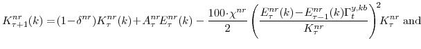
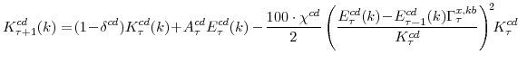
The variable $\epsilon_{t}^{\xi,x}$ is an i.i.d. shock process, and $\rho^{\xi,x}$ represents the persistence of $\Xi^{x}_{t}$ away from steady-state following a shock to equation (14). The household's budget constraint reflects wage setting adjustment costs, which depend on the parameter $\chi^{w}$ and the lagged and steady-state wage inflation rate, and the costs in changing the mix of labor supplied to each sector, which depend on the parameter $\chi^{l}$ . The costs incurred by households when the mix of labor input across sectors changes may be inportant for sectoral comovements, a point we briefly return to when discussing our parameter estimates.

3.5 Monetary Authority

We now turn to the last important agent in our model, the monetary authority. It sets monetary policy in accordance with an Taylor-type interest-rate feedback rule. Policymakers smoothly adjust the actual interest rate $R_{t}$ to its target level $\bar{R}_{t}$

$\displaystyle R_{t} = \left( R_{t-1}\right)^{\phi^{r}} \left( \bar{R}_{t} \right)^{1-\phi^{r}} \exp \left[ \epsilon^{r}_{t} \right],$

(15)

where the parameter $\phi^{r}$ reflects the degree of interest rate smoothing, while $\epsilon_{t}^{r}$ represents a monetary policy shock. The central bank's target nominal interest rate, $\bar{R}_{t}$ depends on GDP growth relative to steady-state growth, $H^{gdp}_{t}/H^{gdp}_{\ast}$ , the acceleration of GDP growth, $H^{gdp}_{t}/H^{gdp}_{t-1}$ , GDP inflation relative to target, $\Pi^{p,gdp}_{\ast}/\Pi^{p,gdp}_{t}$ , and the acceleration of GDP inflation, $\Pi^{p,gdp}_{t}/\Pi^{p,gdp}_{t-1}$ :

$\displaystyle \bar{R}_{t}\!=\!\left(\frac{H^{gdp}_{t}}{H^{gdp}_{\ast}} \right)^{\phi^{h,gdp}} \!\left(\frac{H^{gdp}_{t}}{H^{gdp}_{t-1}}\right)^{\phi^{\Delta h,gdp}} \!\left(\frac{\Pi^{p,gdp}_{t}}{\Pi^{p,gdp}_{\ast}} \right)^{\phi^{\pi,gdp}} \!\left(\frac{\Pi^{p,gdp}_{t}}{\Pi^{p,gdp}_{t-1}} \right)^{\phi^{\Delta\pi,gdp}} \!R_{\ast}.$

(16)

In equation (16), $R_{\ast}$ denotes the economy's steady-state nominal interest rate and $\phi^{h,gdp}$ , $\phi^{\Delta h,gdp}$ , $\phi^{\pi,gdp}$ , and $\phi^{\Delta \pi,gdp}$ denote the weights in the feedback rule.

GDP growth has not yet been discussed. It equals the Divisia (share-weighted) aggregate of final spending in the economy, as given by the identity:

$\displaystyle H^{gdp}_{t}\!= \!\left(\left(\frac{X^{cbi}_{t}}{X^{cbi}_{t-1}}\right)^{P^{cbi}_{\ast}X^{cbi}_{\ast}} \!\!\!\!\left(\frac{X^{kb}_{t}}{X^{kb}_{t-1}}\right)^{P^{kb}_{\ast}X^{kb}_{\ast}} \!\!\!\!\left(\frac{\Gamma^{x,cbi}_{t}\!\!\cdot\widetilde{X}^{gf}_{t}} {\widetilde{X}^{gf}_{t-1}}\right)^{P^{cbi}_{\ast}X^{gf}_{\ast}} \right)^{\frac{1} {P^{cbi}_{\ast}X^{cbi}_{\ast}+P^{kb}_{\ast}X^{kb}_{\ast} +P^{cbi}_{\ast}X^{gf}_{\ast}}} \!\!\!\! \!\!\!\!.$

(17)

In equation (17), $\widetilde{X}^{gf}_{t}$ represent stationary un-modeled output (that is, GDP other than $E^{cnn}_{t}$ , $E^{cd}_{t}$ , $E^{r}_{t}$ , and $E^{nr}_{t}$ ). To a first approximation, this definition of GDP growth is equivalent to how it is defined in the U.S. NIPA. Stationary un-modeled output is exogenous and is assumed to follow the process:

$\displaystyle \ln \widetilde{X}^{gf}_{t}-\ln \widetilde{X}^{gf}_{\ast} =\rho^{x,gf}\left(\ln \widetilde{X}^{gf}_{t}-\ln \widetilde{X}^{gf}_{\ast} \right) +\epsilon^{x,gf}.$

The inflation rate of the GDP deflator, represented by $\Pi^{p,gdp}_{t}$ , is defined implicitly by:

$\displaystyle \Pi^{p,gdp}_{t} H^{gdp}_{t} =\frac{P^{gdp}_{t}X^{gdp}_{t}}{P^{gdp}_{t-1}X^{gdp}_{t-1}} =\frac{P^{cbi}_{t}X^{cbi}_{t}+P^{kb}_{t}X^{kb}_{t}+P^{cbi}_{t}X^{gf}_{t}} {P^{cbi}_{t}X^{cbi}_{t-1}+P^{kb}_{t-1}X^{kb}_{t-1}+P^{cbi}_{t}X^{gf}_{t-1}}.$

3.6 Summary

Our brief presentation of the model highlights several important points. First, although our model considers production and expenditure decisions in a bit more detail, it shares many similar features with other DSGE models in the literature, such as, imperfect competition, nominal price and wage rigidities, and real frictions like adjustment costs and habit persistence. The rich specification of structural shocks (to productivity, preferences, capital efficiency, and mark-ups) and adjustment costs allows our model to be brought to the data with some chance of finding empirical validation.⁵

4 The Estimated Model

The empirical implementation of the model takes a log-linear approximation to the first-order conditions and constraints that describe the economy's equilibrium, casts this resulting system in its state-space representation for the set of (in our case 11) observable variables, uses the Kalman filter to evaluate the likelihood of the observed variables, and forms the posterior distribution of the parameters of interest by combining the likelihood function with a joint density characterizing some prior beliefs. Since we do not have a closed-form solution of the posterior, we rely on Markov-Chain Monte Carlo (MCMC) methods.

The model is estimated using 11 data series. The series, each from the Bureau of Economic Analysis's National Income and Product Accounts except where noted, are: Nominal gross domestic product; Nominal consumption expenditure on nondurables and services excluding housing services; Nominal consumption expenditure on durables; Nominal residential investment expenditure; Nominal business investment expenditure, which equals nominal gross private domestic investment minus nominal residential investment; GDP price inflation; Inflation for consumer nondurables and non-housing services; Inflation for consumer durables; Hours, which equals hours of all persons in the non-farm business sector from the Bureau of Labor Statistics;⁶Wage inflation, which equals compensation per hour in the non-farm business sector from the Bureau of Labor Statistics; and the federal funds rate, from the Federal Reserve Board.

Our implementation adds measurement error processes to the likelihood implied by the model for all of the observed series used in estimation except the nominal interest rate and the aggregate hours series.⁷The model's parameters are reported in the Tables 3 and 4; except where specified, our discussion focuses on parameter values at the posterior mode.

We consider first the parameters related to household-spending decisions. The parameters related to habit-persistence are uniformly large. For nondurables and services excluding housing, the habit parameter is about 0.8, close to the value in found by Fuhrer [2000]. For consumer durables capital the habit parameter is somewhat smaller, while for residential capital it is smaller still. Since most DSGE models do not consider utility functions with this level of disaggregation, there is little consensus on these values. In addition, simulations indicate that habit and adjustment cost parameters--both present in our model--are closely related, further complicating any comparison. Indeed, we estimate investment adjustment costs to be very significant for residential investment but of modest importance for consumer durables.⁸ Nonetheless, habit-persistence and investment adjustment costs are important in generating "hump-shaped" responses of these series to monetary policy shocks.⁹ The estimated value of the remaining preference parameter, the inverse of the labor supply elasticity, is, at a bit over one, a little higher than suggested by the balance of microeconomic evidence (see Abowd and Card [1989]).

With regard to adjustment cost parameters for non-residential investment, we estimate significant costs to the change in investment flows, which imply an elasticity of investment to marginal q of about 1/3. We also find an important role for the sectoral adjustment costs to labor: In our multisector setup, shocks to productivity or preferences in one sector of the economy result in strong shifts of labor towards that sector, which conflicts with the high degree of sectoral co-movement in the data. The adjustment costs to the sectoral mix of labor input ameliorate this potential problem, as in Boldrin et al. [2001].

Finally, adjustment costs to prices and wages are both estimated to be important, although prices appear "stickier" than wages. Our quadratic costs of price and wage adjustment can be translated into frequencies of adjustment consistent with the Calvo model; these are about six quarters for prices and about one quarter for wages. However, these estimates are very sensitive to the specifics of our model and would be altered by reasonable assumptions regarding "real rigidities" such as firm-specific factors or "kinked" demand curves. We find only a modest role for lagged inflation in our adjustment cost specification (around 1/3), equivalent to modest indexation to lagged inflation in other sticky-price specifications. This differs from some other estimates, perhaps because of the focus on a more recent post-1983 sample (similar to results in Kiley [2005b] and Laforte [2005]).

Space constraints prevent a fuller description of the model's properties. A companion paper (Edge, Kiley, and Laforte [2006b]) provides more complete documentation. We summarize some important model properties briefly. As for the sources of aggregate fluctuations in the model, technology shocks--that is, economy-wide productivity shocks, capital goods specific productivity shocks, and shocks to the (non-residential) capital evolution process--explain the overwhelming fraction of output fluctuations. Such shocks are much more important in our DSGE model than in a traditional model such as the Federal Reserve's FRB/US model. We view this as a strength of our model, as the importance of innovations to technology for high frequency fluctuations in output is standard in the academic literature. The addition of a model with this property to the toolkit used in policy analysis can only help expand the range of "stories" considered in forecasting and policy work.

Technology shocks similarly dominate the variance decomposition for inflation at all but the shortest horizons (where transitory markup shocks are important). Shocks to household preferences and to the efficiency of durables consumption spending and residential investment account for relatively little of the variability in the data. Perhaps unsurprisingly, monetary policy shocks contribute very little to the variance decomposition on any variable. Of course, this does not imply that monetary policy is unimportant, as the policy rule has significant effects on model properties. As we will see in the next section, there have been very important discretionary shifts in monetary policy (shocks) over our period, despite the unimportance of this factor overall for variance decompositions.

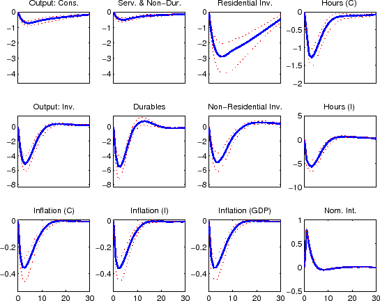
Turning to the response of model variables to fundamental innovations, Figure 2 presents the responses of key variables to a monetary policy shock. In a policy context, it is obviously important that our model capture the conventional wisdom regarding the effects of such shocks, and it is apparent that our model does. In particular, both household and business expenditures on durables (consumer durables, residential investment, and nonresidential investment) respond strongly (and with a hump-shape) to a contractionary policy shock, while nondurables and services consumption display a more muted responses. Each measure of inflation responds gradually albeit probably more quickly than in most analyses based on vector autoregressions.

5 Storytelling with Natural Rate Measures

We now consider some "storytelling" examples from our model. As we emphasized earlier, we view the narratives embedded in our model as a key potential contribution to the forecasting and policymaking process: It is these stories that connect--or possibly disconnect--the output of our model to the intuition and analysis brought to the policymaking process by staff not directly connected to day-to-day model operations. In the context of understanding the historical evolution of natural rate measures in the U.S. economy, we provide several examples of how our model can aid in story-telling. In some cases, the stories told by our DSGE model appear very similar to "conventional" wisdom; in others, the story from our model diverges significantly. This may indicate problems with the conventional wisdom or with our model.

5.1 The Output Gap, Recessions, and Monetary Policy

The first topic we discuss is the evolution of the output gap over our sample period. In our DSGE context, we define the level of potential output as the level that would prevail absent wage and price rigidities and abstracting from shocks to markups. This definition is standard in the new-Keynesian and related DSGE literature (Woodford [2003], Neiss and Nelson [2003]). For comparison purposes, we also consider a measure of potential output and the output gap based on the FRB/US model, which takes a more traditional view of potential output as a smoothly evolving series. In particular, FRB/US potential is based on a production function; total factor productivity in the potential series is a smoothed series for measured total factor productivity (with the smoothing achieved through a Kalman filter on actual TFP); the capital stock in the potential series is the actual measured capital stock; and labor input in the potential series is a smoothed series, more akin to our DSGE model's notion of steady-state labor input.

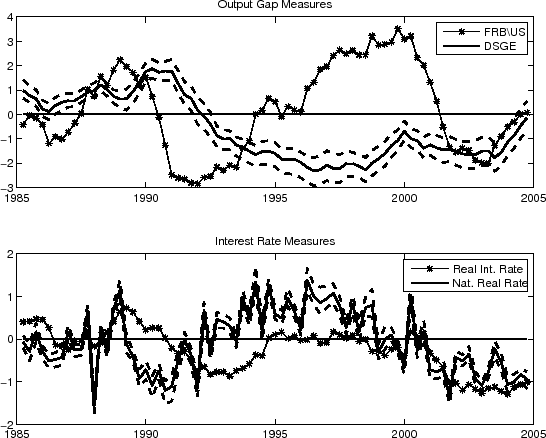
The top panel of Figure 3 graphs the output gap from our model and the FRB/US model's output gap from 1984 to 2004. It is immediately apparent that the two series capture some of the same stories that have been prominent factors in monetary policy decisions over this period. Perhaps most importantly, both series show movements in output away from potential in the early 1990s and in 2001--consistent with the recessions dates around those times documented by the National Bureau of Economic Research (NBER).

One reaction to this finding might be that this is a pretty weak story to hold up as an example illustrating that our DSGE model has some reasonable properties. However, we view the quasi-success of our model in capturing downward movements in the output gap in the neighborhood of NBER recessions as important; additionally, it addresses a criticism that has been made of much simpler new-Keynesian models. In the basic new-Keynesian model with only sticky prices, the output gap is proportional to labor's share of income (see, Woodford [2003]). It is well-known that labor's share of income, in the United States, has tended to rise, or at least not fall sharply, in NBER recessions (see, Rotemberg and Woodford [1999]). This has led some to criticize the new-Keynesian model as failing to connect with basic intuition as to the nature of expansions and contractions (see, Rudd and Whelan [2005]).

Nonetheless, there are sharp differences between the FRB/US and DSGE model generated output gaps, partially reflecting differences in the economic concept captured by the two series. The DSGE model's output gap is a driver of inflation, which implies that the path of inflation has an important bearing on the resulting output-gap path. Two instances illustrating this dependence are the early 1990s, when inflation continued to decline even though a slow recovery was underway (the so-called opportunistic disinflation), and the late 1990s, when inflation remained contained despite the very strong economic growth. These episodes are reflected in the DSGE model's output gap estimate, as this gap remains negative in the early 1990s and for much of the late 1990s. A conceptually similar output gap--albeit one from a reduced-form model of Laubach and Williams [2003]--shows a similar pattern over the 1990s because of the behavior of inflation. The FRB/US output gap measure is, by contrast, less closely linked to inflation:¹⁰ Indeed, real marginal cost, equal to the inverse of the mark-up, is the key driving variable in the model's inflation equation. The FRB/US potential output series is a production function based measure that is built up from smoothed values of multifactor productivity and production inputs. This measure saw output rising above potential through the 1990s.

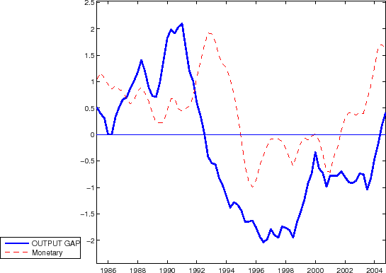
We next turn to the impact of monetary policy during each recession as indicated by the DSGE model. Figure 4 plots the DSGE model's measure of the output gap and the contribution to the output gap of monetary policy shocks, that is, deviations of policy from the standard rule. According to the model, monetary policy shocks acted to raise output toward potential, to a significant extent, in both the early 1990s and from 2001 to 2004.¹¹ This should be unsurprising to even casual observers of policy behavior at that time. But our model says a bit more: when potential output is measured by the efficient level of output, as in DSGE models like ours, it is also possible to state that such discretionary policy shocks were probably welfare-enhancing.

5.2 Potential Output

The view of growth over the past twenty years that emerges from the DSGE model becomes notably different from conventional wisdom once some other issues are considered. The evolution of potential output, and the associated stories regarding the role of technology disturbances in macroeconomic fluctuations, is one important area of disagreement. As noted earlier, our DSGE model attributes the overwhelming majority of fluctuations to technology shocks, where these shocks are total factor productivity shocks or (non-residential) investment efficiency shocks. Models like FRB/US attribute much more of the short-run variation to "animal-spirit" expenditure shocks, typically measured as residuals in the determination of key components of expenditure.

This is apparent in the graph of the output gap in the top panel of Figure 3, which is much smoother in our DSGE model than FRB/US. In terms of overall volatility, our measure of potential (flexible-price) output has a standard deviation of 0.5 percent per quarter--the same level as actual output growth. This implies that the efficient degree of output volatility in the DSGE model is quite close to the actual amount of output volatility. This result may not be particularly surprising given the existing literature on this topic, and Hall [2005] has argued that policymakers should perhaps absorb this lesson by not viewing all economic fluctuations as needing a policy response. So far, however, some policymakers, such as Bean [2005], seem skeptical of this prescription.

The potential for large, high frequency fluctuations in the efficient level of output has been well documented by a substantial literature, from Kydland and Prescott [1982] to modern, new-Keynesian DSGE models with very much a real-business cycle flavor. Given this tradition, this view probably should be represented among the set of models used for policy analysis.

5.3 The Natural Rate of Interest

We now consider the natural rate of interest. Attention to such a concept has surged over the past decade. In the academic community, a significant factor has been the work of Woodford [2003], who provides a elegant overview of monetary policy in the core new-Keynesian model and illustrates the role of the flexible-price equilibrium measure of the real interest rate in policy. For example, in a very simple model with one distortion, policymakers can implement the efficient outcome, with stable inflation, by following a rule that sets the real interest rate equal to its natural rate and promises to respond sufficiently to any move in inflation. While this academic work may have influenced policymakers to some extent, a greater interest in recent years--perhaps attributable to the prolonged period of low real interest rates following the 2001 recession--has been in the "equilibrium" or "neutral" policy rate. In late 2005 and early 2006, it was still common to hear Wall Street economists worrying about the level of the neutral policy rate in the U.S.

The lower panel of Figure 3 presents our DSGE model's measure of the natural rate of interest and the actual real federal funds rate (implied by the actual nominal funds rate and expected inflation from our DSGE model). The natural rate of interest implied by our model is very volatile: its standard deviation is 120 basis points, compared to a standard deviation of the actual real funds rate of only 60 basis points. This outcome is not unexpected: Neiss and Nelson [2003], for example, find similarly volatile estimates of the natural rate of interest for the United Kingdom. From a practical point of view, some policymakers are likely to consider such measures implausible. Based on our experience, policymakers' perceptions as to what the path of the natural real rate should look like are much more akin to something resembling a smoothed path of actual real interest rates. In this respect the natural real interest rate estimates that Laubach and Williams [2003] obtain with their semi-structural Kalman filter model seem more consistent with policymakers' priors than our more volatile measure.

Beyond its plausibility to policymakers, there may be more issues related to fluctuations in the natural rate of interest and their role in the policy process in a typical DSGE model like ours. In particular, our model relies on habit persistence to generate persistent, hump-shaped responses of key expenditure variables to fundamentals. It is well-known that this specification of preferences has some unpalatable asset pricing implications; specifically, these models imply substantial volatility in the risk-free real interest rate (Boldrin et al. [2001]). Given the concerns we expressed earlier regarding habit persistence for other reasons, we view research on quantitative DSGE models that tries to link financial market and business cycle behavior (as started in, for example, Uhlig [2004]) as quite important.

More fundamentally, research examining the movements in actual and natural real interest rates may shed light on the interaction between financial markets and economic activity or the monetary policy process. It has been well-documented that monetary policy appears to smooth the response of nominal interest rates to inflation and output movements. Such a preference for smoothing is present in our policy reaction function, and, in an accounting sense, explains, in part, why actual real rates are less volatile than the measured natural rates. However, this then begs the question of why policymakers smooth nominal interest rates. One reason may be concern about financial stability, which could arise from financial market imperfections that are absent from our model. Inclusion of such frictions may rationalize interest rate smoothing, an important topic for further research.¹²

6 Conclusions

We close by noting some of the practical lessons highlighted by our analysis concerning the use of DSGE models in the policy formulation process and the directions these lessons imply for future research.

The description of movements in potential output generated by our DSGE model highlights how views from the DSGE literature can differ substantially from the "conventional" wisdom of policy practitioners concerning what represents efficient fluctuations in macroeconomic variables. While we have emphasized that alternative views can be a strength of different modeling strategies when the truth is uncertain, we expect that the DSGE model's view that a significant fraction of fluctuations represent the economy's near-efficient response to fundamental shocks will encounter significant resistance from some policymakers. It appears to us that the view in policy circles continues to be one in which a significant fraction of fluctuations is viewed as inefficient; that is, the mainstream view appears to lie much closer to that of Bean [2005] than that of Hall [2005].

This controversy provides one question for future research: How sensitive are our DSGE model's predictions regarding the efficiency of significant high-frequency fluctuations in activity to changes in assumptions regarding the types of shock impinging on the economy or the frictions in certain markets? The efficiency of high-frequency fluctuations would certainly be reduced if disturbances to the degree of distortions in the economy were to increase in importance relative to innovations to technology (and preference) shocks. But estimated DSGE models require much more than simply the theoretical possibility that some alternative shock accounts for high-frequency volatility; they require that such shocks be capable of explaining the patterns observed in the data better than productivity and preference shocks. While it is not immediately obvious how to include a rich set of such shocks to distortions, and whether the data would find a significant role for such shocks if they were included, the practical value of moving the predictions of models closer to the views of policymakers suggests that model developments of this type are an important avenue of research.

The labor market in our DSGE model is clearly one area of the model where additional model frictions could (and indeed should) be added. Our specification of the labor market, while fairly standard in DSGE models, is likely quite incompatible with the concerns of policymakers and the public more generally. Most glaringly, we do not distinguish between the intensive and extensive margins of adjustment for hours, and hence have no meaningful measure of unemployment in our model. Related models have begun to incorporate search or other labor market frictions into DSGE models suitable for monetary policy analysis.

Finally, we alluded in section 6 to concerns regarding financial market behavior in our model. It is quite clear that the nature of financial frictions and the asset pricing implications of any DSGE model are important for monetary policy analysis, as the policy interest rate is one of the economy's key asset prices. Further investigations of model features that help explain financial market, activity, and inflation fluctuations are central to policy discussions, especially given the prominence of asset price and wealth fluctuations on activity in the United States in recent years.

Bibliography

Abowd, J., Card, D., 1989.

On the covariance structure of earnings and hours changes. Econometrica 57, 411-445.

Altig, D., Christiano, C., Eichenbaum M., Linde, J., 2004.

An Estimated Model of US business cycles. Mimeo.

Bean, C., 2005

Comments on: Separating the Business Cycle From Other Economic Fluctuations. In: The Greenspan Era: Lessons for the Future. Federal Reserve Bank of Kansas City.

Bernanke, B., Gertler, M., 1995.

Inside the Black Box: The Credit Channel of Monetary Policy Transmission. Journal of Economic Perspectives 9, 27-48.

Boldrin, M., Christiano, L., Fisher J., 2001.

Habit Persistence, Asset Returns, and the Business Cycle. American Economic Review 91, 149-166.

Christiano, L., Eichenbaum, M., Evans, C., 2005.

Nominal Rigidities and the Dynamic Effects of a Shock to Monetary Policy. Journal of Political Economy 113, 1-45.

DiCecio, R., 2005.

Comovement: It's Not A Puzzle. Federal Reserve Bank of St Louis Working Paper Working Paper 2005-035B.

Dynan, K., 2000.

Habit Formation in Consumer Preferences: Evidence from Panel Data. American Economic Review 90, 391-406.

Edge, R., Laubach, T., Williams, J.C., 2003.

The Responses of Wages and Prices to Techology Shocks. FEDS Working Paper 2003-65.

Edge, R., Kiley, M., Laforte, J.P., 2006a.

A Comparison of Forecast Performance between the FBB Staff Forecasts, Simple Reduced-Form Models, and a DSGE Model. Mimeo.

Edge, R., Kiley, M., Laforte, J.P., 2006b.

Documentation of the 2006 Version of the MAQS DSGE Model of the U.S. Economy. Mimeo.

Erceg, C., Guerrieri, L., Gust, C., 2005.

SIGMA: A new open economy model for policy analysis. Federal Reserve Board International Finance Discussion Paper 835.

Fisher, J., 2006.

The dynamic effects of neutral and investment-specific technology shocks. Journal of Political Economy 114, 413-451.

Fuhrer, J., 2000.

Habit Formation in Consumption and Implications for Monetary-Policy Models. American Economic Review 90, 367-390.

Greenwood, J., Hercowitz, Z., Krusell, P., 1997.

Long-Run Implications of Investment-Specific Technological Change. American Economic Review 8, 342-62.

Greenwood, J., Hercowitz, Z., Krusell, P., 2000.

The Role of Investment-specific Technological Change in the Business Cycle. European Economic Review 44, 91-115.

Hall, R., 2005.

Separating the Business Cycle From Other Economic Fluctuations. In: The Greenspan Era: Lessons for the Future, Federal Reserve Bank of Kansas City.

IMF, 2004.

GEM: A New International Macroeconomic Model. Occasional Paper 239.

Kiley, M., 2005a.

Habit Persistence, Inattention, or Rule-of-Thumb Consumers: Which Accounts for the Predictability of Consumption Growth? Mimeo.

Kiley, M., 2005b.

A Quantitative Comparison of Sticky-Price and Sticky-Information Models of Price Setting. Mimeo.

Kohn, D., 2003.

The Strength in Consumer Durables and Housing: Policy Stabilization or Problem in the Making? Remarks at the Conference on Finance and Macroeconomics. Federal Reserve Bank of San Francisco and SIEPR, February 28.

Kydland, F., Prescott, E., 1982.

Time-to-build and Aggregate Fluctuations. Econometrica 50, 1345-70.

Laforte, J., 2005.

Pricing Models: A Bayesian DSGE Approach to the U.S. Economy. Mimeo.

Laubach, T., Williams, J., 2003.

Measuring the Natural Rate of Interest. Review of Economics and Statistics 85, 1063-1070.

Neiss, K., Nelson, E., 2003.

The Real Interest Rate Gap as an Inflation Indicator. Macroeconomic Dynamics 7, 239-62.

Reifschneider, D., Stockton, D., Wilcox, D., 1997.

Econometric Models and the Monetary Policy Process. Carnegie-Rochester Conference Series on Public Policy 47, 1-37.

Rotemberg, J., Woodford, M., 1999.

The Cyclical Behavior of Marginal Cost. In: Taylor, J., Woodford, M. (Eds.), Handbook of Macroeconomics, Amsterdam: North-Holland.

Rudd, J., Whelan, K., 2005a.

Does Labor's Share Drive Inflation? Journal of Money, Credit, and Banking 37, 297-312.

Smets, F., Wouters, R., 2004a.

Comparing Shocks and Frictions in the US and Euro Area Busines Cycles: A Bayesian DSGE Approach. European Central Bank, Working Paper No.391.

Smets, F., Wouters, R., 2004b.

Shocks and Frictions in the US Busines Cycles: A Bayesian DSGE Approach. Mimeo.

Uhlig, H., 2004.

Macroeconomics and Asset Markets: Some Mutual Implications. Mimeo.

Whelan, K., 2003.

A Two-Sector Approach to Modeling U.S. NIPA Data. Journal of Money, Credit and Banking 35, 627-56.

Woodford, M., 2003.

Interest and Prices: Foundations of a Theory of Monetary Policy. Princeton University Press.

Table 1: Average Growth and Relative Price Changes (1984q1 to 2004q4).
	Average Real Growth Rate	Average Nominal Growth Rate	Average Price Change*
Consumer non-durable goods and non-housing services	3 1/4 percent	6 1/4 percent	n.a.
Consumer housing services	2 1/2 percent	6 1/4 percent	3/4 percent
Consumer durable goods	6 3/4 percent	6 1/2 percent	-3 percent
Res. investment goods	3 3/4 percent	7 1/2 percent	1/2 percent
Non-res. investment goods	6 1/4 percent	6 1/4 percent	-2 3/4 percent

*Relative to cons. non-durable goods & non-housing services prices.Return to Table

Table 2: Cross Correlations: GDP and Major Private Expenditure Components
	-4	-3	-2	-1	0	+1	+2	+3	+4
Cons. non-dur. goods & non-hous. services	-0.03	0.08	0.23	0.28	0.43	0.37	0.28	0.28	0.18
Cons. dur. goods	0.10	0.06	0.14	0.25	0.32	0.06	0.06	0.08	0.07
Res. inv. goods	0.15	0.19	0.34	0.31	0.44	0.15	- 0.08	- 0.12	- 0.15
Non-res. inv. goods	0.12	0.01	0.17	0.14	0.61	0.31	0.26	-0.09	-0.02

**Table 3:** Calibrated Parameters
$\beta$	$\alpha$	$\psi$	$\delta^{nr}$	$\delta^{cd}$	$\delta^{r}$	$\Theta^{x,cbi}_{\ast}$	$\Theta^{x,kb}_{\ast}$	$\Theta^{l}_{\ast}$	$\Gamma^{z,m}_{\ast}$	$\Gamma^{z,kb}_{\ast}$	$H^{x,gf}_{\ast}$
0.990	0.260	5	0.030	0.055	0.004	7.000	7.000	7.000	1.003	1.004	0.250

**Table 4:** Prior and Posterior Distributions
Param.	Prior Type	Prior Mean	Prior S.D.	Posterior Mode	Posterior S.D.	Posterior 10th perc.	Posterior 50th perc.	Posterior 90th perc.
$h^{cnn}$	B	0.500	0.122	0.766	0.048	0.707	0.770	0.828
$h^{cd}$	B	0.500	0.122	0.571	0.196	0.372	0.600	0.919
$h^{r}$	B	0.500	0.122	0.500	0.128	0.328	0.490	0.665
$\nu$	G	2.000	1.000	1.287	0.735	0.805	1.554	2.600
$\chi^{p}$	G	2.000	1.000	2.331	0.808	2.294	3.193	4.338
$\eta^{p}$	B	0.500	0.224	0.257	0.124	0.163	0.313	0.481
$\chi^{w}$	G	2.000	1.000	1.555	1.478	1.268	2.750	4.944
$\eta^{w}$	B	0.500	0.224	0.296	0.147	0.138	0.328	0.529
$\chi^{nr}$	G	2.000	1.000	0.831	0.397	0.676	1.053	1.665
$\chi^{cd}$	G	2.000	1.000	0.145	0.082	0.055	0.181	0.275
$\chi^{r}$	G	6.000	1.000	10.198	2.590	8.085	10.852	14.793
$\chi^{l}$	G	2.000	1.000	0.766	1.703	0.412	1.366	3.615
$\eta^{l}$	B	0.500	0.224	0.779	0.202	0.377	0.702	0.910
$r^{\pi}$	N	2.000	1.000	3.532	0.515	2.947	3.561	4.251
$r^{\triangle{\pi}}$	N	0.500	0.400	-0.041	0.080	-0.137	-0.040	0.070
$r^{h,gdp}$	N	0.500	0.400	0.210	0.026	0.183	0.216	0.250
$r^{\triangle{h,gdp}}$	N	0.500	0.400	-0.084	0.025	-0.124	-0.092	-0.059
$\rho^r$	B	0.750	0.112	0.900	0.018	0.876	0.902	0.922
$\rho^{a,nr}$	B	0.750	0.112	0.894	0.032	0.839	0.884	0.920
$\rho^{a,cd}$	B	0.750	0.112	0.842	0.115	0.619	0.802	0.908
$\rho^{a,r}$	B	0.500	0.150	0.527	0.103	0.379	0.519	0.648
$\rho^{\xi,cnn}$	B	0.750	0.112	0.795	0.079	0.660	0.778	0.867
$\rho^{\xi,cd}$	B	0.750	0.112	0.899	0.080	0.733	0.859	0.931
$\rho^{\xi,r}$	B	0.750	0.112	0.793	0.113	0.615	0.787	0.907
$\rho^{\xi,l}$	B	0.750	0.112	0.940	0.030	0.884	0.930	0.962
$\rho^{\gamma,m}$	B	0.500	0.150	0.305	0.079	0.211	0.315	0.418
$\rho^{\gamma,kb}$	B	0.750	0.112	0.927	0.051	0.823	0.903	0.949
$\rho^{x,gf}$	B	0.750	0.112	0.982	0.014	0.957	0.978	0.990

Notes:

B denotes the Beta distribution; G denotes the Gamma distribution; and N denotes the Normal distribution.
For the Gamma distribution, hyperparameters are shown.
The prior and posterior distributions for the variances of the model's shock processes are given in Edge, Kiley, and Laforte [2006b].

Figure 1: Model Overview

Notes:

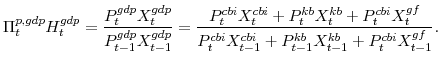
CBI represents the economy's slow growing sector, so denoted because consumption [C] goods and services account for most of its output and it is produced by the business and institutions [BI] sector of the economy.
KB represents the economy's fast growing sector, so denoted because its output is capital [K] goods and it is produced by the business [B] sector of the economy.

Figure 2: Impulse Responses: Monetary Policy Shock

Notes:

The dotted lines are the 90 percent credible set.

Figure 3: Key Measures

Notes:

The real interest rate and natural real rate are shown relative to their steady-state level.
The solid lines are the median estimates of the output gap and natural real rate.
The dotted lines are the 90 percent credible set around the output gap and natural real rate.

Natural Rate Measures in an Estimated DSGE Model of the U.S. Economy

January 30, 2007

4 The Estimated Model

5 Storytelling with Natural Rate Measures

6 Conclusions

Figure 1: Model Overview

Figure 2: Impulse Responses: Monetary Policy Shock

Figure 3: Key Measures

Figure 4: Output Gap: Historical Decomposition and Monetary Policy Contribution