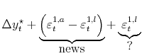
News, Noise, and Estimates of the "True" Unobserved State of the Economy
Keywords: GDP, statistical discrepancy, news and noise, signal-to-noise ratios, optimal combination of estimates, business cycles
Abstract:
Which provides a better estimate of the "true" state of the U.S. economy, gross domestic product (GDP) or gross domestic income (GDI)? Past work has assumed the difference between each estimate and the "true" state of the economy is pure noise, taking greater variability to imply lower reliability. We posit instead that each difference may be pure news; then greater variability implies higher information content and greater reliability. This is a general point, applicable to numerous situations beyond the case of combining GDP and GDI. For that particular case, we analyze various vintages of estimates, developing models for combining GDP and GDI under the differing assumptions, and use revisions to show the news assumption is probably more accurate.
JEL classification: C1, C82.
1 Introduction
For analysts of economic fluctuations, estimating the true state of the economy from imperfectly measured official statistics is an ever-present problem. As most economists agree that no one statistic is a perfect gauge of the state of the economy, many have proposed using some type of weighted
average of multiple imperfectly measured statistics instead. Examples include the composite index of coincident indicators,1 and averages of different measures
of aggregate economic activity such as gross domestic product (GDP) and its income-side counterpart GDI. While the precise meaning of the state of the economy can vary from case to case, in this paper we take it to mean the growth rate of the size of the economy as traditionally defined in the U.S.
National Income and Product Accounts (NIPAs).2![]() 3
3
The main point of our paper is as follows. To our knowledge, all prior attempts to produce such a weighted average of imperfectly measured statistics have made a strong implicit assumption that drives their weighting: that the difference between the true state of the economy and each measured statistic is pure noise, or completely uncorrelated with information about the true state of the economy.4 Under this assumption, a statistic with greater idiosyncratic variance is given a smaller weight because it is assumed to contain more noise. We examine a different assumption that produces a diametrically opposite weighting: that the difference between the true state of the economy and each measured statistic is pure news, or pure information about the true state of the economy. Under this assumption, a statistic with greater idiosyncratic variance is given a larger weight because it is assumed to contain more news about the true state of the economy.
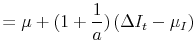
Focusing on GDP and GDI allows us to make this basic point in a simple bivariate context. These two measures of the size of the U.S. economy would equal one another if all the transactions in the economy were observed, but measurement difficulties lead to the statistical discrepancy between the two; their quarterly growth rates often diverge significantly. Weale (1992) and others5 have estimated the growth rate of "true" unobserved GDP as a combination of measured GDP growth and GDI growth, generally concluding that GDI growth should be given more weight than measured GDP growth. Is GDI really the more accurate measure`? We argue for caution, as the results are driven entirely by the noise assumption: the models implicitly assume that since GDP growth has higher variance than GDI growth over their sample period, it must be noisier, and so should receive a smaller weight. However GDP may have higher variance because it contains more information about "true" unobserved GDP (this is the essence of the news assumption); then measured GDP should receive the higher weight.
In section 2 of the paper, we emphasize that since we never observe the "true" state of the economy, assumptions about news vs. noise are inherently untestable. In the general version of our model that allows the idiosyncratic component of each measured statistic to be a mixture of news and noise, virtually any set of weights can be rationalized by making untestable assumptions about the mixtures. More information must be brought to bear on the problem; otherwise the choice of weights will be arbitrary. This point is broadly applicable, extending well beyond the simple bivariate case of GDP and GDI. For example, a large and growing literature on dynamic factor models uses principal components or other methods to extract common factors out of large data sets; see Stock and Watson (2002), Forni, Hallin, Lippi, and Reichlin (2000), Bernanke and Boivin (2003), Giannone, Reichlin, and Small (2005), Bernanke, Boivin, and Eliasz (2005), and Boivin and Ng (2006).6 While often these common factors are used for pure forecasting, sometimes they are equated with unobserveables of interest, assuming the idiosyncratic components of the variables in the dataset are uninteresting noise. However if these idiosyncratic components do contain useful information about the unobserveables of interest, estimating the unobserveables optimally may require taking weighted averages of the variables in the dataset very different from those implied by the factor models.
While this fundamental indeterminancy - the arbitrary nature of most weighting schemes - is somewhat disturbing, in the case of combining GDP and GDI we bring more information to bear on the problem to help pin down what the weights should be. In particular, an examination of revisions is helpful; section 3 summarizes this evidence, which favors the assumption that the idiosyncratic components of GDP growth and GDI growth are mostly news. Section 4 of the paper estimates the models and computes "true" unobserved GDP growth under the different assumptions, accounting for the fact that the variance of the measured estimates drops dramatically after the early 1980s - see McConnell and Perez-Quiros (2000). The results distinguish between the first few releases of GDP and GDI, and the later more heavily-revised estimates that are typically used for historical research. For the first few releases, the variance of measured GDP growth exceeds the variance of GDI growth, so the news assumption we favor dictates that measured GDP should receive the higher weight. However, for the later vintages of estimates we find the reverse: GDI growth has higher variance than measured GDP growth.7 When combining these estimates, the news assumptions would place the higher weight on GDI.
Our empirical results on GDP and GDI are interesting from a couple of perspectives. First, our explicit treatment of different vintages of GDP growth and GDI growth should be of interest to those tracking the current state of the economy in real time. Revisions can have important effects on the properties of these growth rates, but the unrevised (or little revised) growth rates are what analysts must employ in real time. Our results show how to combine these unrevised growth rates that are typically available, producing better real time measures of the growth rate of the U.S. economy; that is, measures that both account for revisions and are based on sound statistical assumptions. These improved real time measures could be useful for many purposes, including monetary policy. Second, our empirical results on combining the heavily-revised estimates of GDP and GDI growth should be of interest to those who estimate real business cycle and other models where moments of the economy's growth rate are important. For example, under our preferred news model assumptions, the variance of estimated "true" GDP growth exceeds the variance of measured GDP growth, and represents a lower bound on the actual variance of "true" GDP growth. The common practice of using the variance of measured GDP growth alone, then, underestimates the true variability of the economy's growth rate if the news model assumptions are true, a fact with clear implications for real business cycle, asset pricing, and other models. This and some other conclusions are drawn in section 5 of the paper.
2.1 Review of News, Noise, and Covariance Assumptions
Let
![]() be the true growth rate of the economy, let
be the true growth rate of the economy, let
![]() be one of its measured estimates, and let
be one of its measured estimates, and let
![]() be the difference between the two, so:
be the difference between the two, so:
In contrast, if an estimate
![]() were constructed efficiently with respect to a set of information about
were constructed efficiently with respect to a set of information about
![]() (call it
(call it
![]() ), then
), then
![]() would be the conditional expectation of
would be the conditional expectation of
![]() given that information set:
given that information set:
Writing:
the term
The news model can be written with the notation of the noise model if we take
![]() and switch this term to the other side of the equation, but the covariance assumption of the noise model will be violated; in fact the error will be perfectly
negatively correlated with the missing piece of information about the true growth rate of the economy, so
and switch this term to the other side of the equation, but the covariance assumption of the noise model will be violated; in fact the error will be perfectly
negatively correlated with the missing piece of information about the true growth rate of the economy, so
![]() . The variance ordering of the news assumption,
. The variance ordering of the news assumption,
![]() , will still hold, as:
, will still hold, as:
Writing the models in this common notation, and differentiating them by assumptions about the covariance of
The pure news and pure noise assumptions are extremes; many intermediate cases could be considered where
![]() is part news and part noise, implying differing degrees of negative covariance between
is part news and part noise, implying differing degrees of negative covariance between
![]() and
and
![]() . We consider a general model that encompasses these intermediate cases in the next subsection.
. We consider a general model that encompasses these intermediate cases in the next subsection.
2.2 The Mixed News and Noise Model
We consider a model with two estimates of true unobserved GDP, each an efficient estimate plus noise:
The noise components
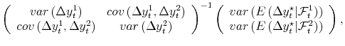
To clearly illustrate the main points of the paper, we focus on the simple case where all variables are jointly normally distributed, and where measured GDP and GDI are serially uncorrelated.10 With normality, the conditional expectation of the true growth rate of the economy is a weighted average of GDP and GDI; netting out means yields:
| (1') |
calling the conditional expectation
| (2') |  |
|
|
|
using
It is useful to introduce some additional notation. Call the covariance between the two estimates ![]() ; this arises from the overlap between the information sets used to compute the
efficient estimates.11 The model imposes the condition that the variance of each estimate is at least as large as the covariance between the two; then let
; this arises from the overlap between the information sets used to compute the
efficient estimates.11 The model imposes the condition that the variance of each estimate is at least as large as the covariance between the two; then let
![]() and
and
![]() be the variances of the
be the variances of the
![]() and
and
![]() , respectively. The idiosyncratic variance in each estimate, the
, respectively. The idiosyncratic variance in each estimate, the ![]() for
for ![]() , arises from two potential sources. The first is the idiosyncratic news in each estimate - the information in each efficient estimate missing from the other.
The second source of idiosyncratic variance is the noise,
, arises from two potential sources. The first is the idiosyncratic news in each estimate - the information in each efficient estimate missing from the other.
The second source of idiosyncratic variance is the noise,
![]() .
.
Let the fraction of idiosyncratic variance in the ![]() th estimate that is news be
th estimate that is news be ![]() , so
, so
![]() is the variance of idiosyncratic news in
is the variance of idiosyncratic news in
![]() , and
, and
![]() is the variance of noise. This
is the variance of noise. This ![]() will range from
zero, the case where the idiosyncratic variation in the estimate is pure noise, to one, the case where that variation is pure news. Then equation (2) becomes:
will range from
zero, the case where the idiosyncratic variation in the estimate is pure noise, to one, the case where that variation is pure news. Then equation (2) becomes:
|
 |
Solving and substituting into (2) gives:
 |
|||
| (3') | 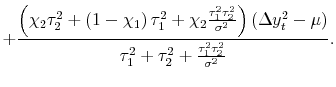 |
To understand this formula, it is helpful to work through some special cases of interest.
First note that not all of the parameters in this model are identified. We observe three moments from the variance-covariance matrix of
![]() , which is not enough to pin down the five parameters
, which is not enough to pin down the five parameters ![]() ,
, ![]() ,
, ![]() ,
, ![]() and
and ![]() . Imposing values for
. Imposing values for ![]() and
and ![]() will allow identification of the remaining parameters, and previous attempts to estimate models of this kind have focused on one particular
imposition, namely
will allow identification of the remaining parameters, and previous attempts to estimate models of this kind have focused on one particular
imposition, namely
![]() . The implication is that the two information sets must coincide, at least in the universe of information that is relevant for predicting
. The implication is that the two information sets must coincide, at least in the universe of information that is relevant for predicting
![]() , so
, so
![]() . Then the difference between each estimate and the truth,
. Then the difference between each estimate and the truth,
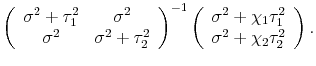
![]() , is pure noise. We call the general model with these assumptions the pure noise model, and under this model equation (3) becomes:12
, is pure noise. We call the general model with these assumptions the pure noise model, and under this model equation (3) becomes:12
| (4') |  |
In the pure noise model, the weight for one measure is proportional to the idiosyncratic variance of the other measure - since the idiosyncratic variance in each estimate is assumed to be noise, the "noisier" measure is downweighted. The weights on the (net of mean) estimates sum to less than
one; as is typical in the classical measurement error model, coefficients on noisy explanatory variables are downweighted. In fact, as the common variance ![]() approaches zero, the
signal-to-noise ratio in the model approaches zero as well, and the formula instructs us to give up on the estimates of GDP and GDI for any given time period, using the overall sample mean as the best estimate for each and every period.
approaches zero, the
signal-to-noise ratio in the model approaches zero as well, and the formula instructs us to give up on the estimates of GDP and GDI for any given time period, using the overall sample mean as the best estimate for each and every period.
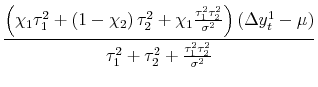
The opposite case is what we call the pure news model, where
![]() . The difference between each estimate and the truth,
. The difference between each estimate and the truth,
![]() , is pure news or pure information in this case, as in the second example in the previous subsection. Equation (3) then becomes:
, is pure news or pure information in this case, as in the second example in the previous subsection. Equation (3) then becomes:
| (5') |  |
The weight for each measure is now proportional to its own idiosyncratic variance - the estimate with greater variance contains more news and hence receives a larger weight. In addition, the weights (on the net of mean estimates) sum to a number greater than unity, another result diametrically opposed to that of the noise model. As
Moving back to the more general model, note that adding ![]() to equation (3) yields a weighted average of the growth rate of GDP, the growth rate of GDI, and
to equation (3) yields a weighted average of the growth rate of GDP, the growth rate of GDI, and ![]() ; the weights on these three variables sum to one. However in some situations the econometrician may have little confidence in the estimated mean
; the weights on these three variables sum to one. However in some situations the econometrician may have little confidence in the estimated mean ![]() , so it may be inadvisable to use it as the third component in the weighted average. One way around this problem is to force the weights on
, so it may be inadvisable to use it as the third component in the weighted average. One way around this problem is to force the weights on
![]() and
and
![]() to sum to one, with
to sum to one, with
![]() ; substituting into (1) and rearranging yields an expectation that can be computed without knowledge of
; substituting into (1) and rearranging yields an expectation that can be computed without knowledge of ![]() :
:
| (6') |
Adding back in
| (3') |  |
With the assumptions of the pure noise model, this particular estimator is equivalent to the estimator proposed by Weale (1992), who applied to the case of GDP and GDI the techniques developed earlier in Stone et al (1942). Appendix B clarifies the relation between these earlier estimators and those derived here.
Finally, consider another case of interest. If
![]() and
and
![]() , then
, then
![]() and
and
![]() . Placing all the weight on any given estimate amounts to an assumption that the idiosyncratic portion of that estimate is pure news, and the idiosyncratic portion of the other
estimate is pure noise. If placing all the weight on either variable can be justified in this way, perhaps any set of weights could be justified. This turns out to be the case. Let the ratio of the weights
. Placing all the weight on any given estimate amounts to an assumption that the idiosyncratic portion of that estimate is pure news, and the idiosyncratic portion of the other
estimate is pure noise. If placing all the weight on either variable can be justified in this way, perhaps any set of weights could be justified. This turns out to be the case. Let the ratio of the weights
![]() , so:
, so:
| (7) |  |
where we've expressed
One set of weights is as justifiable as any other; without further information about the estimates, the choice of weights will be arbitrary. In the empirical work below on GDP and GDI, we do bring further information to bear on the problem, and examine whether the pure news or pure noise model is closer to reality.
3 Data: The Case of GDP and GDI
The most widely-used statistic produced by the U.S. Bureau of Economic Analysis (BEA) is GDP, its expenditure-based estimate of the size of the economy; this statistic is the sum of personal consumption expenditures, investment, government expenditures, and net exports. However the BEA also produces an income-based estimate of the size of the economy, gross domestic income (GDI), from different information. National income is the sum of employee compensation, proprietors' income, rental income, corporate profits and net interest; adding consumption of fixed capital and a few other balancing items to national income produces GDI.13 Computing the value of GDP and GDI would be straightforward if it were possible to record the value of all the underlying transactions included in the NIPA definition of the size of the economy, in which case the two measures would coincide. However all the underlying transactions are not recorded: the BEA relies on various surveys, censuses and administrative records, each imperfect, to compute the estimates, and differences between the data sources used to produce GDP and GDI, as well as other measurement difficulties, lead to the statistical discrepancy between the two measures.
Table 1 summarizes the sequence of vintages of quarterly GDP and GDI data released by the BEA. The "advance" estimate for the most current quarter is released about a month after the quarter closes, with the "preliminary" estimate following a month after "advance" and the "final"
estimate following a month after "preliminary"; these three vintages are sometimes called the current quarterly estimates of GDP and GDI.14 Usually in the
summer of year ![]() , all quarters of year
, all quarters of year ![]() are reopened for the first annual
revision, and those quarters are revised again in the second and third annual revisions in years
are reopened for the first annual
revision, and those quarters are revised again in the second and third annual revisions in years ![]() and
and ![]() . Finally, about every five years, all of the accounts data are reopened for benchmark (comprehensive) revisions. The benchmarks are a mixture of methodological changes, statistical changes, and the incorporation of previously unavailable data, mainly from the most
recent quinquennial economic census.
. Finally, about every five years, all of the accounts data are reopened for benchmark (comprehensive) revisions. The benchmarks are a mixture of methodological changes, statistical changes, and the incorporation of previously unavailable data, mainly from the most
recent quinquennial economic census.
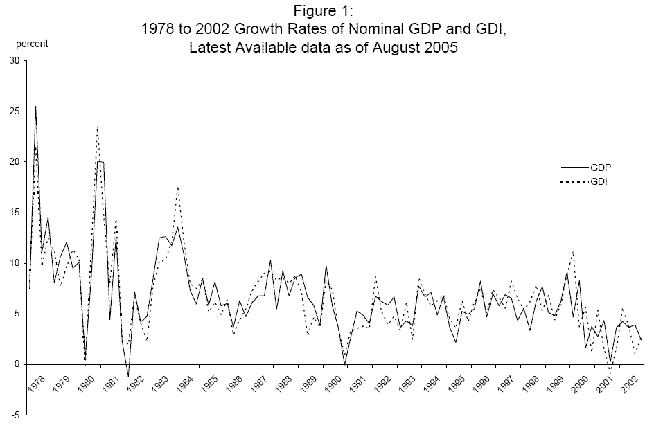
The BEA maintains a database of each of these vintages of estimates for GDP, GDI, and various sub-components, extending back to 1978; our sample extends from this date through 2002.15Our "latest available" data series were pulled from the BEA web site in August 2005; figure 1 plots the annualized quarterly growth rates of these nominal GDP (solid line) and nominal GDI (dashed line) numbers. These nominal data reflect relatively high inflation in the US in the late 1970s and early 1980s, and past research has documented the evident decline in volatility of the economy's growth rate sometime around 1984.16
Before reporting the summary statistics for our data, some additional notation is helpful. Let
![]() be the difference between "true" GDP growth and the "advance" estimate of measured GDP growth;
be the difference between "true" GDP growth and the "advance" estimate of measured GDP growth;
![]() is the difference between "true" GDP growth and its "preliminary" estimate, and so forth, with
is the difference between "true" GDP growth and its "preliminary" estimate, and so forth, with
![]() being the difference between "true" GDP growth and its latest available estimate. So:
being the difference between "true" GDP growth and its latest available estimate. So:
Each revision incorporates more comprehensive and accurate source data; Grimm and Weadock (2006) estimate that only 45% of the needed source data are available for the "advance" GDP estimate, improving to 75% for the "preliminary" estimate and 78% for the "final" estimate. For the first annual revision, about 95% of the data are available, although these data are not all available at the quarterly frequency, so the BEA must resort to interpolation and other techniques. The remainder of the data arrives at the subsequent annual and comprehensive benchmark revisions, although data incorporated at benchmarks are available only every five years. It should be noted that these latter flows contain informative revisions to previously received source data. Given these facts, we assume each revision brings the estimates closer to the truth
This assumption that the revisions are news is consistent with the flow of source data, and how the BEA uses the data to compute its estimates. When the BEA lacks data on components of GDP and GDI in its earlier vintages of estimates, they often substitute either related data or "trend extrapolations," assuming the growth rate for the current quarter is equal to the average growth rate over the past several quarters or years. Such extrapolations will generally have low variance, and when the BEA receives and substitutes actual data for these extrapolated components, the variance of the growth rates will increase. The new source data on some components of GDP and GDI is part of the news in each revision.
Table 2 reports summary statistics on means and variances of growth rates of GDP and GDI, for different vintages. The BEA does not produce "advance" estimates of GDI, as corporate profits and some other data are unavailable that close to the end of the quarter, and while the BEA does produce "preliminary" GDI for the first to third quarters of the year, it does not do so for the fourth. Consequently, we do not report GDI results for these vintages.
The results in table 2 are broadly consistent with the revisions to GDP and GDI being news. The first panel shows that over the full 1978 to 2002 sample, the variances of both GDP and GDI growth increase as the data pass through each revision; the only exception is the second annual revision. The second panel reports results for the 1984Q3 to 2002 sub-sample, excluding the high-variance, high-inflation period in our data.17 The drop in overall variance in this panel is clearly evident. Looking across vintages, the variance of GDP growth grows less uniformly than in the first panel; the revisions to GDI, in contrast, still look very much like news. The last row in each of these first two panels reports covariances between GDP growth and GDI growth, the other crucial ingredient in our combining formulas. Since 1984Q3, this covariance generally declines as the data pass through revisions; the next section discusses this phenonomenon.
The lower two panels of table 2 report means and variances of revisions - the first column reports means and variances of
![]() , for example. Measured by variance, the largest revisions occur moving from "final" current quarterly vintage to first annual revision vintage, and in the
benchmarks that move from third annual to latest (at least over the full sample). It should be kept in mind that what we call the revision from the third annual to the latest is actually the sum of multiple benchmark revisions for most years in the sample.
, for example. Measured by variance, the largest revisions occur moving from "final" current quarterly vintage to first annual revision vintage, and in the
benchmarks that move from third annual to latest (at least over the full sample). It should be kept in mind that what we call the revision from the third annual to the latest is actually the sum of multiple benchmark revisions for most years in the sample.
Table 3 sheds some additional light on whether revisions to GDP and GDI are news or noise, following Mankiw and Shapiro (1986) in showing a correlation matrix of each revision with each vintage. If the revisions are news, they should be uncorrelated with vintages prior to the revision, and
should be positively correlated with the current and subsequent vintages. For example, if the revision
![]() is news, it will be correlated with
is news, it will be correlated with
![]() ,
,
![]() , and later vintages, but not
, and later vintages, but not
![]() . If the revision
. If the revision
![]() is news, it will be correlated with
is news, it will be correlated with
![]() ,
,
![]() , and later estimates, but not
, and later estimates, but not
![]() or
or
![]() . Under the noise model, the exact opposite is true. The correlation table represents a compactly-expressed horse race between the two models.
. Under the noise model, the exact opposite is true. The correlation table represents a compactly-expressed horse race between the two models.
Panels A and B of table 3 show results for GDP and GDI using the full 1978 to 2002 sample; the numbers in parentheses below the correlation estimates are t-statistics. A large number of statistically significant coefficients appear in the upper right-hand section of each panel, and zero in the lower left-hand section, evidence again consistent with the revisions being news. Panels C and D report results for the 1984Q3 to 2002 sub-sample; as in table 2, the evidence in favor of the revisions being news is somewhat less uniform here for GDP, but remains strong for GDI.
Two points should be kept in mind about this evidence indicating that revisions to GDP and GDI are largely news, not noise. First, if each revision brings the estimates closer to
![]() , at least part of the difference between each early vintage estimate and "true" unobserved GDP is news, not noise. Taking the "advance" GDP estimate as an example, the
difference between this estimate and "true" GDP growth,
, at least part of the difference between each early vintage estimate and "true" unobserved GDP is news, not noise. Taking the "advance" GDP estimate as an example, the
difference between this estimate and "true" GDP growth,
![]() , can be decomposed in the following way:
, can be decomposed in the following way:
 |
This first component in the above equation - the component of
Our second point is more speculative, as inferences about the
![]() and conclusions about how to combine the fully-revised, latest-available estimates of GDP and GDI are more difficult to draw. However, in our judgment, it seems
reasonable to draw at least tentative inferences based on the revisions evidence. The argument is based on the assumption that observed patterns would continue: if the BEA did ultimately acquire exact knowledge of "true" unobserved GDP, we hypothesize that its (hypothetical) ultimate revision
from the most current estimates to the truth would be similar to other revisions we have observed in the past. After examining six types of revisions and finding each one to be mostly news, it seems more probable than not that this hypothetical ultimate revision would be news as well. This point is
bolstered by the fact that there are still large data gaps on both sides of the accounts at the quarterly frequency even after benchmark revisions, as these revisions incorporate data at the much-lower quinquennial frequency. To deal with these missing quarterly-frequency data, the BEA uses
interpolation and other techniques similar to those employed to handle missing data in its earlier-vintage estimates such as current quarterly. The similarity of the techniques probably leads to a similar outcome: estimates with lower variance than what would obtain if more information were
available.
and conclusions about how to combine the fully-revised, latest-available estimates of GDP and GDI are more difficult to draw. However, in our judgment, it seems
reasonable to draw at least tentative inferences based on the revisions evidence. The argument is based on the assumption that observed patterns would continue: if the BEA did ultimately acquire exact knowledge of "true" unobserved GDP, we hypothesize that its (hypothetical) ultimate revision
from the most current estimates to the truth would be similar to other revisions we have observed in the past. After examining six types of revisions and finding each one to be mostly news, it seems more probable than not that this hypothetical ultimate revision would be news as well. This point is
bolstered by the fact that there are still large data gaps on both sides of the accounts at the quarterly frequency even after benchmark revisions, as these revisions incorporate data at the much-lower quinquennial frequency. To deal with these missing quarterly-frequency data, the BEA uses
interpolation and other techniques similar to those employed to handle missing data in its earlier-vintage estimates such as current quarterly. The similarity of the techniques probably leads to a similar outcome: estimates with lower variance than what would obtain if more information were
available.
4 Estimates of "True" Unobserved GDP
Table 4 reports maximum likelihood estimates of the pure news and pure noise models for the different vintages of nominal GDP and GDI growth. Figure 1 makes it clear that breaks in the means and variances of these series are appropriate.18 We employed likelihood-ratio tests allowing for breaks in some parameters over potential points in the middle ![]() of the sample - see Andrews (1993). Allowing for breaks in
of the sample - see Andrews (1993). Allowing for breaks in ![]() produces massive increases in the likelihood function, with the greatest increase occuring with a
1984Q3 break for all five vintages of data. Allowing for a break in
produces massive increases in the likelihood function, with the greatest increase occuring with a
1984Q3 break for all five vintages of data. Allowing for a break in ![]() at the same point as the break in
at the same point as the break in ![]() (the visual evidence in Figure 1 indicates that these two breaks were roughly coincident), again produces the greatest likelihood increase with the 1984Q3 break for all five vintages. Evidence for further breaks in
(the visual evidence in Figure 1 indicates that these two breaks were roughly coincident), again produces the greatest likelihood increase with the 1984Q3 break for all five vintages. Evidence for further breaks in ![]() and
and ![]() was mixed; the table reports results where these idiosyncratic variances were held constant throughout
the sample.19
was mixed; the table reports results where these idiosyncratic variances were held constant throughout
the sample.19
The likelihood function is the same for both models; only the formulae for the weights to be placed on GDP and GDI differ. The first panel of table 4 reports parameter estimates (with standard errors beneath in parentheses) and the weights for the news model renormalized so they sum to one as in
(3'). These weights are unaffected by the parameter breaks in ![]() . The second panel reports the unrestricted weights for both models in the post-break period. In addition, we report the
variance of the predicted values for "true" GDP growth for each model. For the pure news model, we interpret this quantity as a lower bound on the variance of true GDP growth. Writing:
. The second panel reports the unrestricted weights for both models in the post-break period. In addition, we report the
variance of the predicted values for "true" GDP growth for each model. For the pure news model, we interpret this quantity as a lower bound on the variance of true GDP growth. Writing:
| (8) |
the
Most important for the relative weights on GDP and GDI are the idiosyncratic variances ![]() and
and ![]() . For the final current quarterly estimates, the variance of GDP exceeds the variance of GDI. Under the noise model assumptions where variance is a bad, GDI receives the higher weight; under the news model assumptions where variance is a good, GDP receives the higher
weight. Of course, the news model assumptions should be favored here, as the evidence in section 3 favorable to the news model is most relevant for these current quarterly estimates. The standard errors for the weights are somewhat large in this case, however.
. For the final current quarterly estimates, the variance of GDP exceeds the variance of GDI. Under the noise model assumptions where variance is a bad, GDI receives the higher weight; under the news model assumptions where variance is a good, GDP receives the higher
weight. Of course, the news model assumptions should be favored here, as the evidence in section 3 favorable to the news model is most relevant for these current quarterly estimates. The standard errors for the weights are somewhat large in this case, however.
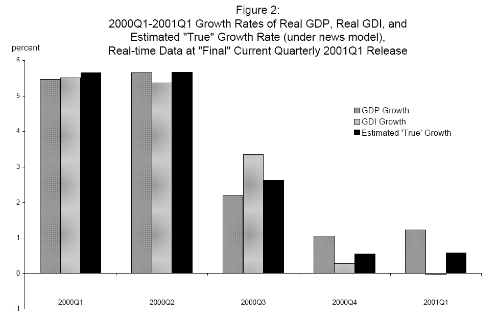
In tracking the current state of the economy in real time, the early-vintage estimates are what is available, and so the state of the economy must be inferred from them. Consider the GDP and GDI growth rates that were available after BEA's quarterly data release at the end of June 2001, when final current quarterly vintage growth rates prevailed from 2000Q1 to 2001Q1. These are plotted in Figure 2 along with estimated "true" GDP growth from the news model, with weights estimated using the real time data on final current quarterly vintage growth rates through 2001Q1. The estimated weights for (net of mean) nominal GDP growth and nominal GDI growth are 0.60 and 0.46, respecively; after adding back the mean, the combined estimate is deflated by the GDP deflator available in real time (as are the raw GDP growth and GDI growth series plotted). The combined estimate is about a half a percentage point below measured real GDP growth in both 2000Q4 and 2001Q1.20 Such differences may seem small, but even marginal improvements in the accuracy of real time estimates of the growth rate of the economy can be important. In this case, for example, a half a percentage point difference over two quarters might aid inferences about whether or not the economy is in recession; in the Markov switching model in Nalewaik (2007a), the additional information provided by GDI growth, beyond that contained in GDP growth, was crucial to recognizing the start of the 2001 recession in real time. Incorporating our new estimates of "true" GDP growth into such a Markov switching model would be an interesting avenue for future research.
Moving to later vintage estimates, Table 4 shows that the idiosyncratic variance of GDI relative to GDP grows as the data pass through annual revisions. Since these revisions are largely news, a plausible intepretation is that the informativeness of GDI relative to GDP is growing as we pass through annual and benchmark revisions. In other words, a greater amount of useful information is incorporated into GDI at revisions, causing larger increases in its variance. This interpretation is consistent with the findings in Nalewaik (2007a, 2007b), who shows that although GDI appears to be more informative than GDP in recognizing recessions (or, more precisely, more informative in recognizing the state of the world in a two-state Markov switching model for the economy's growth rate), most of that greater information content comes from the information in annual and benchmark revisions.
It is curious that the idiosyncratic variances grow as we move forward in vintage while, post 1984, the common variance ![]() falls; GDP and GDI become less similar as the data pass
through the revisions. Although this may seem to contradict the assumption that both GDP and GDI move closer to the truth as they pass through revisions, consider again how the BEA constructs its estimates. For the earliest vintages, the data available to the BEA are quite limited (see section 3),
and for this reason there is substantial overlap in the source data used to compute GDP and GDI. For example, data on much of services consumption, an expenditure-side component, are missing at the time of the current quarterly estimates, so the BEA borrows data from the income-side, using
employment, hours and earnings as a substitute for many sub-components of services. In later vintages, when more complete and appropriate data on the components of GDP and GDI becomes available, the overlap between the two measures becomes smaller; the two measures diverge, even as each one
individually moves closer to true unobserved GDP growth.
falls; GDP and GDI become less similar as the data pass
through the revisions. Although this may seem to contradict the assumption that both GDP and GDI move closer to the truth as they pass through revisions, consider again how the BEA constructs its estimates. For the earliest vintages, the data available to the BEA are quite limited (see section 3),
and for this reason there is substantial overlap in the source data used to compute GDP and GDI. For example, data on much of services consumption, an expenditure-side component, are missing at the time of the current quarterly estimates, so the BEA borrows data from the income-side, using
employment, hours and earnings as a substitute for many sub-components of services. In later vintages, when more complete and appropriate data on the components of GDP and GDI becomes available, the overlap between the two measures becomes smaller; the two measures diverge, even as each one
individually moves closer to true unobserved GDP growth.
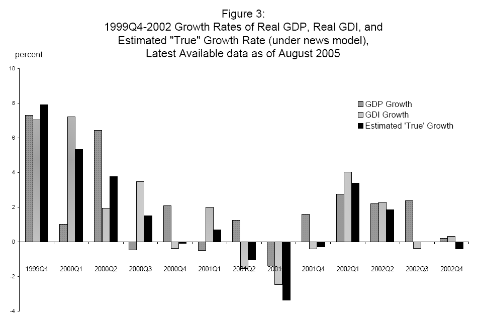
Some of this divergence between the two measures can be seen by comparing Figure 2 to Figure 3, which plots 1999-2002 growth rates of the latest available data on GDP and GDI (as of August 2005) with estimated "true" GDP from the news model; as before, these nominal data have been deflated by the GDP deflator. These latest available data show erratic patterns in GDP and GDI growth in 2000 that were not present in the final current quarterly growth rates shown in Figure 2. In contrast, the combined estimates based on the latest available data show a smooth downward trend into recession. However this apparent smoothness in Figure 3 should not mislead the reader, as the variance of estimated "true" GDP growth exceeds the variance of both GDP growth and GDI growth. Consider the fourth quarter of 1999 (the quarter with the fastest late-cycle growth), when "true" GDP growth exceeds the growth rate of both GDP and GDI, and the third quarter of 2001 (the nadir of the recession), when "true" GDP growth is below each estimate. These examples are not surprising, as the news model weights more heavily the component series with higher variance and uses weights that sum to more than one. And if the news model is true, this relatively large variance represents a lower bound on the variance of "true" GDP growth, a fact with potentially important implications for a wide class of economic models that depend importantly on the variance of the growth rate of the economy, for example many real business cycle and asset pricing models.
5 Conclusions
This paper makes a general point about heretofore implicit assumptions involved in taking weighted averages of imperfectly measured statisics, and uses insights from that general point to develop new models for estimating aggregate economic activity - what we have called "true" unobserved GDP - as a weighted average of measured GDP and GDI. These two measures should coincide in principle as they attempt to measure the same thing, but because of differences in source data they do not. Combining them in some way may produce an estimate that is superior to either one in isolation; however previous attempts to do so have made the strong implicit assumption that the difference between "true" GDP and each measured statistic is pure noise, or completely uncorrelated with "true" GDP. Our work allows for the possibility that the difference between "true" GDP and each measured statistic is partly or pure news, or correlated with "true" GDP. If this is true, then our models may weight more heavily the statistic with higher variance, as it could contain more information about "true" GDP, in contrast to previous models, which always weight less heavily the statistic with higher variance, as it is assumed to contain more measurement error.
We provide evidence that the BEA's numerous revisions to GDP and GDI are largely news, showing that at least part of the differences between "true" GDP and the first few estimates of GDP and GDI are news. We argue further on the basis of continuity that the differences between "true" GDP and the more-heavily-revised vintages of GDP and GDI are likely news as well. However this evidence is not definitive; some uncertainty about "true" unobserved GDP will always remain. As such, some type of Bayesian combining of the different models may be a promising way to proceed in future research, or Minimax estimation over the unidentified parameters of our general news and noise model, perhaps incorporating the evidence on revisions presented in this paper into prior distributions.21
Our empirical results have clear uses for analysts of the current state of the economy and business cycles, as we show how to combine the unrevised estimates of GDP and GDI growth that are typically available in real time, using solidly-grounded statistical assumptions. This is in contrast to prior work, which often ignores revisions, and has been based on statistical assumptions that are arbitrary. In addition, our results on combining the latest available GDP and GDI estimates have important implications for many economic models. If the news hypothesis is true, we show that the true variance of the growth rate of the economy is not equal to the variance of measured GDP growth, as is often assumed in real business cycle, asset pricing, and other models; the true variance is actually higher.
While our empirical results focus on GDP and GDI, some type of news model applies more generally whenever the goal is to combine the information in multiple efficiently-constructed estimates of a variable, each based on incomplete and non-identical information. Furthermore, the news vs. noise considerations highlighted here are ubiquitous when attempting to estimate unobserveables. Take the well known index of coincident indicators as constructed by Stock and Watson (1989), used by Diebold and Rudebusch (1996) and many other economists. Stock and Watson decompose each of four time series into a common factor plus an idiosyncratic component; a time series that covaries relatively less with the other three will receive less weight in the common factor and have higher idiosyncratic variance. Stock and Watson define the state of the economy as this common factor, so a series with greater (relative) idiosyncratic variance receives less weight in this construct. Is this best weighting? There may be good reasons to define the state of the economy as this common factor, following the venerable tradition of Burns and Mitchell (1946). However if we define the state of the economy as something other than this common factor, the answer to this question is unclear: if the idiosyncratic components of the time series are noise, the Stock and Watson approach is appropriate, but if the idiosyncratic components are news, then time series that contain much idiosyncratic variation are uniquely informative about the state of the economy, and should be weighted more heavily.
This same point is applicable to the burgeoning literature on dynamic factor models using large datasets. For example, Bernanke et al (2005) equate linear combinations of common factors with four unobserved variables: (1) the output gap, (2) a cost-push shock, (3) output, and (4) inflation. They take these last two as unobserveable due to measurement difficulties, in the same spirit as our work here. However it is unlikely that the idiosyncratic components of all 120 time series they use to extract the common factors are uncorrelated with these four unobserveables. For example, our results indicate that information from the income side of the national accounts probably contains useful information about the growth rate of output, above and beyond the information contained in expenditure-side variables. So it may be possible to improve the results in Bernanke et al (2005) with modifications such as allowing the idiosyncratic information in their employment and income variables to be correlated with unobservables (1) or (3).
These examples illustrate that the noise assumption is often implicit in models of imperfect measurement (in state space models often entering through the assumed orthogonality of the errors of the observation equations with the errors of the state equations); a contribution of this paper is to pull this hidden assumption out into the open, so that economists and statisticians can thoroughly assess its validity. Seemingly innocuous econometric assumptions can imply that the difference between truth and measurement is noise; econometric estimators generally treat variance as a bad, and the noise assumption does as well. We have examined some circumstances for which this assumption may be inappropriate, where it is possible that variance should be treated as a good instead. While realizing this leads to some fundamental indeterminancies, our work here has taken some initial steps towards deriving estimators appropriate for handling these situations.
We will consider two efficient estimates of true GDP growth, one based on consumption growth, and the other based on the growth rate of investment. After constructing each efficient estimate, we will discuss how to produce the improved estimate of true GDP growth by combining them with equation (5).
Let
![]() ,
,
![]() ,
,
![]() , and
, and
![]() be the contributions to true GDP growth
be the contributions to true GDP growth
![]() of consumption, investment, government, and net exports, so:
of consumption, investment, government, and net exports, so:
For simplicity, we will examine the case where neither
The relation between
![]() and
and
![]() determines the nature of the efficient estimates and weights on
determines the nature of the efficient estimates and weights on
![]() and
and
![]() in equation (5). Consider first the case where these variables are independent. Then:
in equation (5). Consider first the case where these variables are independent. Then:
There is no information common to
Next consider the case where
![]() and
and
![]() are perfectly correlated, so:
are perfectly correlated, so:
 |
Given that
Finally consider the general linear case. In this case:
Least squares projections tell us that
The variance parameters of the news model are identified from the following relations:
Substituting
It should be pointed out that, when combining
![]() and
and
![]() in this particular example, using equation (5) is not the most natural way to proceed. An easier and more intuitive procedure would be to set
in this particular example, using equation (5) is not the most natural way to proceed. An easier and more intuitive procedure would be to set
![]() to zero in
to zero in
![]() , set
, set
![]() to zero in
to zero in
![]() , and then combine, producing:
, and then combine, producing:
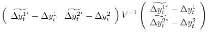
Equation (3') with the pure noise assumptions yields
![]() , essentially the estimator presented in Weale (1992).23 This paper applied to the case of U.S. GDP and GDI the techniques developed in Stone, Champernowne, and Meade (1942) and Byron (1978); see also Weale (1985), and Smith, Satchell, and
Weale (1998). In the general case, Stone et al (1942) considered a row vector of estimates
, essentially the estimator presented in Weale (1992).23 This paper applied to the case of U.S. GDP and GDI the techniques developed in Stone, Champernowne, and Meade (1942) and Byron (1978); see also Weale (1985), and Smith, Satchell, and
Weale (1998). In the general case, Stone et al (1942) considered a row vector of estimates ![]() that should but do not satisfy the set of accounting constraints
that should but do not satisfy the set of accounting constraints ![]() . They produce a new set of estimates
. They produce a new set of estimates
![]() that satisfy the constraints by solving the constrained quadratic minimization problem:
that satisfy the constraints by solving the constrained quadratic minimization problem:
| (B.1) | |||
| S.T. |
The matrix
 |
|
||
| S.T. |
Substituting the constraint into the objective function, we have:
| (B.2) | 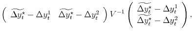 |
with
 |
Solving the quadratic minimization problem with this
Problem (B2) is a different minimization problem than the least squares minimization problems that we solve in this paper, where we solve for the weights in (1) or (6) and then compute the predicted values
![]() ; problem (B2) solves for
; problem (B2) solves for
![]() directly, leaving the weights implicit. In solving for the weights in (1) or (6), assumptions must be made about the covariances between
directly, leaving the weights implicit. In solving for the weights in (1) or (6), assumptions must be made about the covariances between
![]() and the estimates
and the estimates
![]() , whereas in (B2) assumptions must be made about
, whereas in (B2) assumptions must be made about ![]() ; as we have seen,
when these assumptions are equivalent and when some constraints are applied to (1), the two approaches can give the same result. Comparing the Stone, Champernowne, and Meade (1942) approach with the approach taken here, in a more general setting such as in (B1), is beyond the scope of this paper,
but is another interesting avenue for future research.
; as we have seen,
when these assumptions are equivalent and when some constraints are applied to (1), the two approaches can give the same result. Comparing the Stone, Champernowne, and Meade (1942) approach with the approach taken here, in a more general setting such as in (B1), is beyond the scope of this paper,
but is another interesting avenue for future research.
| Vintage | Variable Name |
|---|---|
| Advance Current Quarterly |
|
| Preliminary Current Quarterly |
|
| Final Current Quarterly |
|
| First Annual Revision |
|
| Second Annual Revision |
|
| Third Annual Revision |
|
| Latest Available |
|
| Measure |
|
|
|
|
|
|
|
|---|---|---|---|---|---|---|---|
| GDP mean | 6.22 | 6.41 | 6.46 | 6.50 | 6.54 | 6.63 | 6.74 |
| GDP variance | 11.55 | 12.73 | 13.19 | 14.38 | 14.21 | 14.88 | 16.18 |
| GDI mean | 6.55 | 6.60 | 6.67 | 6.66 | 6.75 | ||
| GDI variance | 12.60 | 13.91 | 13.59 | 14.07 | 15.86 | ||
| covariance(GDP,GDI) | 12.46 | 13.57 | 13.14 | 13.27 | 14.03 |
| Measure |
|
|
|
|
|
|
|
|---|---|---|---|---|---|---|---|
| GDP mean | 5.17 | 5.34 | 5.32 | 5.37 | 5.42 | 5.47 | 5.56 |
| GDP variance | 3.62 | 4.07 | 4.24 | 4.40 | 4.24 | 4.50 | 4.31 |
| GDI mean | 5.48 | 5.48 | 5.56 | 5.54 | 5.58 | ||
| GD variance | 3.92 | 4.48 | 4.51 | 5.12 | 5.51 | ||
| covariance(GDP,GDI) | 3.70 | 3.76 | 3.49 | 3.41 | 3.32 |
| Measure |
|
|
|
|
|
|
|---|---|---|---|---|---|---|
| GDP mean | 0.20 | 0.04 | 0.04 | 0.05 | 0.08 | 0.11 |
| GDP variance | 0.69 | 0.16 | 1.35 | 0.72 | 0.52 | 1.56 |
| GDI mean | 0.05 | 0.07 | -0.01 | 0.09 | ||
| GDI variance | 1.56 | 1.07 | 0.98 | 2.04 |
| Measure |
|
|
|
|
|
|
|---|---|---|---|---|---|---|
| GDP mean | 0.17 | -0.02 | 0.05 | 0.05 | 0.05 | 0.08 |
| GDP variance | 0.43 | 0.11 | 1.06 | 0.59 | 0.46 | 0.71 |
| GDI mean | 0.00 | 0.08 | -0.03 | 0.05 | ||
| GDI variance | 1.27 | 1.00 | 0.89 | 0.78 |
| Revision |
|
|
|
|
|
|
|
|---|---|---|---|---|---|---|---|
|
|
0.09 | 0.32 | 0.31 | 0.30 | 0.34 | 0.32 | 0.27 |
|
|
(0.87) | (3.30) | (3.27) | (3.09) | (3.56) | (3.36) | (2.75) |
|
|
0.11 | 0.11 | 0.22 | 0.19 | 0.18 | 0.14 | 0.08 |
|
|
(1.07) | (1.07) | (2.18) | (1.89) | (1.80) | (1.42) | (0.79) |
|
|
-0.01 | -0.01 | -0.02 | 0.29 | 0.26 | 0.24 | 0.13 |
|
|
(-0.11) | (-0.12) | (-0.18) | (2.98) | (2.66) | (2.43) | (1.31) |
|
|
-0.15 | -0.10 | -0.10 | -0.14 | 0.08 | 0.09 | 0.05 |
|
|
(-1.46) | (-0.98) | (-1.02) | (-1.39) | (0.84) | (0.87) | (0.52) |
|
|
0.09 | 0.07 | 0.05 | 0.02 | 0.03 | 0.21 | 0.20 |
|
|
(0.85) | (0.70) | (0.49) | (0.23) | (0.28) | (2.17) | (2.07) |
|
|
0.16 | 0.12 | 0.10 | -0.00 | -0.03 | -0.03 | 0.28 |
|
|
(1.59) | (1.20) | (0.97) | (-0.03) | (-0.26) | (-0.26) | (2.94) |
| Revision |
|
|
|
|
|
|---|---|---|---|---|---|
|
|
-0.03 | 0.31 | 0.26 | 0.25 | 0.16 |
|
|
(-0.28) | (3.21) | (2.72) | (2.51) | (1.64) |
|
|
-0.13 | -0.18 | 0.10 | 0.07 | 0.05 |
|
|
(-1.31) | (-1.82) | (0.98) | (0.73) | (0.48) |
|
|
-0.03 | -0.04 | -0.07 | 0.20 | 0.07 |
|
|
(-0.26) | (-0.43) | (-0.67) | (1.99) | (0.65) |
|
|
0.15 | 0.08 | 0.07 | -0.02 | 0.34 |
|
|
(1.52) | (0.81) | (0.65) | (-0.24) | (3.53) |
| Revision |
|
|
|
|
|
|
|
|---|---|---|---|---|---|---|---|
|
|
0.01 | 0.33 | 0.37 | 0.35 | 0.35 | 0.28 | 0.23 |
|
|
(0.07) | (3.00) | (3.37) | (3.19) | (3.21) | (2.49) | (2.04) |
|
|
-0.04 | 0.04 | 0.21 | 0.14 | 0.13 | 0.07 | -0.01 |
|
|
(-0.37) | (0.38) | (1.79) | (1.22) | (1.08) | (0.60) | (-0.12) |
|
|
-0.20 | -0.20 | -0.21 | 0.28 | 0.23 | 0.18 | 0.16 |
|
|
(-1.76) | (-1.71) | (-1.86) | (2.49) | (2.00) | (1.60) | (1.35) |
|
|
-0.16 | -0.16 | -0.16 | -0.23 | 0.14 | 0.18 | 0.14 |
|
|
(-1.39) | (-1.34) | (-1.38) | (-2.04) | (1.17) | (1.53) | (1.17) |
|
|
0.03 | -0.04 | -0.06 | -0.12 | -0.07 | 0.25 | 0.19 |
|
|
(0.24) | (-0.31) | (-0.53) | (-1.02) | (-0.58) | (2.21) | (1.63) |
|
|
-0.05 | -0.09 | -0.12 | -0.16 | -0.20 | -0.25 | 0.15 |
|
|
(-0.43) | (-0.78) | (-1.06) | (-1.37) | (-1.77) | (-2.21) | (1.28) |
| Revision |
|
|
|
|
|
|---|---|---|---|---|---|
|
|
-0.16 | 0.38 | 0.27 | 0.20 | 0.14 |
|
|
(-1.38) | (3.51) | (2.42) | (1.77) | (1.22) |
|
|
-0.12 | -0.23 | 0.24 | 0.23 | 0.20 |
|
|
(-0.99) | (-1.99) | (2.14) | (1.97) | (1.71) |
|
|
0.00 | -0.07 | -0.07 | 0.35 | 0.26 |
|
|
(0.02) | (-0.56) | (-0.58) | (3.19) | (2.26) |
|
|
0.10 | 0.02 | -0.01 | -0.10 | 0.28 |
|
|
(0.89) | (0.17) | (-0.05) | (-0.82) | (2.49) |
| Vintage | 1978Q1-1984Q2: |
1978Q1-1984Q2: |
1984Q3-2002Q4: |
1984Q3-2002Q4: |
News Model:
|
News Model:
|
||
|---|---|---|---|---|---|---|---|---|
| Final Curr. Qtrly. | 9.62 | 24.74 | 5.43 | 3.62 | 0.59 | 0.28 | 0.68 | 0.32 |
| Final Curr. Qtrly. (standard error) | (0.98) | (7.13) | (0.23) | (0.63) | (0.23) | (0.22) | (0.25) | (0.25) |
| First Annual | 9.74 | 28.41 | 5.43 | 3.75 | 0.59 | 0.58 | 0.50 | 0.50 |
| First Annual (standard error) | (1.05) | (8.31) | (0.23) | (0.67) | (0.25) | (0.25) | (0.20) | (0.20) |
| Second Annual | 9.77 | 27.63 | 5.48 | 3.49 | 0.70 | 0.82 | 0.46 | 0.54 |
| Second Annual (standard error) | (1.04) | (8.10) | (0.23) | (0.64) | (0.28) | (0.29) | (0.17) | (0.17) |
| Third Annual | 9.89 | 27.74 | 5.50 | 3.44 | 1.02 | 1.36 | 0.43 | 0.57 |
| Third Annual (standard error) | (1.04) | (8.17) | (0.23) | (0.67) | (0.36) | (0.38) | (0.14) | (0.14) |
| Latest Available | 10.08 | 30.23 | 5.57 | 3.06 | 1.40 | 2.54 | 0.35 | 0.65 |
| Latest Available (standard error) | (1.09) | (8.61) | (0.23) | (0.67) | (0.53) | (0.61) | (0.13) | (0.13) |
| Vintage | Noise Model: |
Noise Model: |
Noise Model:
|
News Model: |
News Model: |
News Model:
|
|---|---|---|---|---|---|---|
| Final Curr. Qtrly. | 0.30 | 0.65 | 3.49 | 0.70 | 0.35 | 4.36 |
| Final Curr. Qtrly. (standard error) | (0.23) | (0.25) | (0.23) | (0.25) | ||
| First Annual | 0.46 | 0.47 | 3.53 | 0.54 | 0.53 | 4.70 |
| First Annual (standard error) | (0.19) | (0.19) | (0.19) | (0.19) | ||
| Second Annual | 0.49 | 0.42 | 3.20 | 0.51 | 0.58 | 4.75 |
| Second Annual (standard error) | (0.16) | (0.15) | (0.16) | (0.15) | ||
| Third Annual | 0.49 | 0.37 | 2.98 | 0.51 | 0.63 | 5.44 |
| Third Annual (standard error) | (0.13) | (0.12) | (0.13) | (0.12) | ||
| Latest Available | 0.50 | 0.27 | 2.39 | 0.50 | 0.73 | 6.41 |
| Latest Available (standard error) | (0.12) | (0.09) | (0.12) | (0.09) |