
Insider Rates vs. Outsider Rates in Lending
The presence of private information about a firm can affect the competition among potential lenders. In the Sharpe (1990) model of information asymmetry among lenders (with the von Thadden (2004) correction), an uninformed outside bank faces a winner's curse when competing with an informed inside bank. This paper examines the model's prediction for observed interest rates at an inside vs. outside bank. Although the outside bank wins more bad firms than the inside bank, the winner's curse also causes the outside rate conditional on firm type to be lower in expectation than the inside rate conditional on firm type. I show analytically that the expected interest rate at the outsider can be either higher or lower than the expected interest rate at the insider, depending on the net of these two effects. Under the assumption that the banks split the firms in a tie bid, a numerical solution shows that the outside expected interest rate is higher than the inside expected interest rate for high quality borrower pools, but the outside expected interest rate is lower for low quality borrower pools.
JEL Classifications: G21, C72, D44, D82
* Please address comments to Lamont K. Black, Mail Stop 153, Federal Reserve Board, 20th & C Streets N.W., Washington, DC 20551, tel: (202) 452-3152, fax: (202) 452-5295, email: [email protected].
The opinions expressed do not necessarily reflect those of the Federal Reserve Board or its staff. I would like to thank Allen Berger, Ken Brevoort, Rochelle Edge, Eric Leeper, Robert Marquez, Richard Rosen, and Greg Udell for helpful comments and discussions. All remaining errors are my own.
1. Introduction
Sometimes banks have different amounts of information about a firm when competing for a loan. In this situation, the presence of private information will affect the level of competition among potential lenders, which will in turn affect observed interest rates. The issue is important for understanding the predicted outcome of competition between the informed bidding of insider banks and the uninformed bidding of outsider banks. Although intuition may suggest that the expected interest rate1 will be higher at an outside lender due to the "winner's curse," this paper shows that the apparent intuition is not always correct in a standard framework of insider vs. outsider lending. Depending on borrower characteristics, the expected interest rates at an outside lender may be higher or lower than the expected interest rates at an inside lender.
The standard theoretical framework used in this paper is the Sharpe (1990) model of inside and outside banks. In the Sharpe model, a bank learns private information about a firm through the process of lending. This bank becomes the "inside" bank in subsequent bidding on a new loan for the firm, whereas all other lenders without private information are "outside" banks. In the second period of the model, when banks compete for the firm's loan, the inside bank has an informational advantage over all the outside banks. A correction to the Sharpe paper by von Thadden (2004) shows that there is no pure-strategy equilibrium. Both the inside and outside bank offer rates from mixed strategies and the firm chooses the lowest offer.2
In this model of inside vs. outside lending, the outsider faces a clear winner's curse problem. This problem is due to the adverse selection present in the probability of the outside bank winning the bid. If both banks were equally informed, each bank would know which firms are the bad firms. However, in this model, the outside lender has an informational disadvantage. Even though the outsider chooses a mixed strategy so that it has some possibility of winning a good firm, the outsider's informational disadvantage increases the probability of the outsider winning a bad firm.
The winner's curse would seem to imply that the expected interest rate at the outside bank is higher. If the outside bank wins more bad firms than the inside bank and bad firms have to pay a higher interest rate than good firms, the comparison of insider vs. outsider rates seems clear. Von Thadden (2004) states that the prediction of the model is a higher expected interest rate at the outsider.3 However, the following analysis shows that this universal conclusion is premature. An additional effect of the winner's curse is that the inside bank is able to extract greater rents from the good firms and the outside bank underprices the bad firms. Combining the probabilities of winning and the expected interest rates for each firm reveals a surprising result. This paper shows that, in some cases, the expected interest rate at the inside bank is higher than the expected interest rate at the outside bank. Therefore, the Sharpe model does not provide a universal prediction of whether the inside or outside expected interest rate is higher.
This paper shows numerically that the prediction of the model depends on the parameters of the model, which are the borrower characteristics. The results indicate that the outside expected interest rate is higher than the inside expected interest rate for high-quality borrower pools and the inside expected interest rate is higher than the outside expected interest rate in low-quality borrower pools. This suggests that the prediction of the theory for average observed interest rates when firms switch depends on the characteristics of the borrowers in the sample, which is an important point of clarification for future empirical work on switching.
The remainder of the paper is laid out as follows. Section 2 provides a brief overview of the model. Section 3 provides the theoretical predictions of the model for the probabilities of each lender winning and discusses the sensitivity of the results to the assumption about tie bids. Section 4 analyzes the expected interest rates for three cases of lender competition. Section 5 discusses the winner's curse. Section 6 analyzes analytically the sign of the difference between the inside and outside rate and Section 7 analyzes this difference numerically over the parameter space. Section 8 concludes.
2. The Model
In the Sharpe model, there are two qualities of firms, ![]() , with probabilities of project success
, with probabilities of project success ![]() . The proportion of high quality firms is
. The proportion of high quality firms is ![]() . For the entire pool of borrowers, the probability of success is
. For the entire pool of borrowers, the probability of success is
![]() , such that
, such that ![]() . Banks all have this same
public information when bidding for firm loans in period 1 and firms do not know their own quality. After the bidding process in the first period, one bank makes a loan to the firm and becomes the "inside" bank. This inside bank receives a private signal
. Banks all have this same
public information when bidding for firm loans in period 1 and firms do not know their own quality. After the bidding process in the first period, one bank makes a loan to the firm and becomes the "inside" bank. This inside bank receives a private signal ![]() about the quality of the firm, based on the firm's performance on the first loan. If the firm succeeds on the first loan, the inside bank receives a signal of
about the quality of the firm, based on the firm's performance on the first loan. If the firm succeeds on the first loan, the inside bank receives a signal of ![]() , and if the firm fails on the first loan, the inside bank receives a signal of
, and if the firm fails on the first loan, the inside bank receives a signal of ![]() . This private information received by the inside bank allows the
inside bank to distinguish between "good" firms (an
. This private information received by the inside bank allows the
inside bank to distinguish between "good" firms (an ![]() signal) and "bad" firms (an
signal) and "bad" firms (an ![]() signal). The probability of a success in the second period conditional on success in the first period is
signal). The probability of a success in the second period conditional on success in the first period is
![]() , where
, where
![]() . Likewise, conditional on failure in the first period, the probability of success in the second period is
. Likewise, conditional on failure in the first period, the probability of success in the second period is ![]() . These conditional probabilities of success can be expressed in simplified form as
. These conditional probabilities of success can be expressed in simplified form as
which follow the order of
The "outside" banks are the banks that did not lend to the firm and did not receive the private signal. In the second stage of the model, the bidding is between the inside bank and an outside bank. The inside bank conditions its bid on its private signal, while the outside bank only has public information.4 Von Thadden (2004) shows that the inside bank and outside bank both choose a mixed strategy for their bids. The analysis in this paper is based on Proposition 2 of the von Thadden paper:
The outside bank's equilibrium strategy has a point mass of
Proposition 2 establishes the bidding functions of both the inside and outside bank.
The inside bank has a different bidding strategy for each firm type. For ![]() firms, the inside bank bids from
firms, the inside bank bids from ![]() , a distribution of rates
, a distribution of rates
![]() . Because the good signal about the firm is not public information, the firm always pays more than
. Because the good signal about the firm is not public information, the firm always pays more than ![]() . For
. For ![]() firms, the inside bank bids
firms, the inside bank bids ![]() , which is
the zero-profit loan rate. The inside lender cannot extract rents from the worse of the two types.
, which is
the zero-profit loan rate. The inside lender cannot extract rents from the worse of the two types.
The outside bank has the same bidding strategy for all firms. It does not know each firm's type, so it cannot have two different bidding strategies for the two different firm types, but it knows that the inside bank has private information. If the outside bank were to offer a single rate for all
firms, the outside bank would lose the bid for all the good firms and win the bid for all the bad firms. To mitigate this winner's curse, the outside bank chooses a mixed bidding strategy. The outside bank bids from ![]() with probability
with probability ![]() and bids
and bids ![]() with
probability
with
probability ![]() .
.
The important part of the model is the competition between the insider and outsider. The contribution of this paper is to analyze the outcome of these bidding strategies. Because the inside bank has a different bidding strategy for each of the two firm types, the next section begins by comparing competition by firm type.
3. The Probabilities of the Insider or Outsider Winning
This section analyzes the probabilities of winning for the inside and outside bank. The analysis is first done separately for each of the two firm types. These probabilities are then combined to show the probability of winning for the inside and outside bank, unconditional on firm type.
The probability of the inside or outside bank winning an ![]() firm follows from the bidding process for
firm follows from the bidding process for ![]() firms. When the firm is an
firms. When the firm is an ![]() firm, the inside bank always makes an offer from
firm, the inside bank always makes an offer from ![]() . The outside bank makes an offer from
. The outside bank makes an offer from ![]() with probability
with probability ![]() and an offer of
and an offer of ![]() with probability
with probability ![]() . This implies the
following probabilities of winning for the inside and outside bank, conditional on the firm being an
. This implies the
following probabilities of winning for the inside and outside bank, conditional on the firm being an ![]() firm:
firm:
where the subscript
The probability of the inside or outside bank winning an ![]() firm follows from the bidding process for
firm follows from the bidding process for ![]() firms. When the firm is an
firms. When the firm is an ![]() firm, the inside bank always offers
firm, the inside bank always offers ![]() . The outside bank makes an offer from
. The outside bank makes an offer from ![]() with a probability
with a probability ![]() or an offer of
or an offer of ![]() with probability
with probability ![]() .
.
At this point in the analysis, the assumption about which bank wins in the event of a tie bid becomes relevant. One of the seemingly unimportant aspects of the Sharpe (1990) model is the assumption that the inside bank wins the loan in the event of a tie bid. This assumption would be unimportant in the case of continuous bidding functions; however, the bidding functions of both firms have a point mass at the highest rate. Altering this assumption can affect the comparison of inside vs. outside rates. The rest of the paper proceeds under the assumption that the inside and outside bank split the loans in the event of a tie bid.5
The probabilities of winning for the inside and outside bank, conditional on the firm being an ![]() firm, are:
firm, are:
For these firms, when the outside bank makes an offer from
The probability of each bank winning, unconditional on firm type, can be calculated by combining the probability of winning a particular firm type with the proportion of each firm type. The proportion of good and bad firms depends simply on the probabilities of firms succeeding or failing in the
first period. A firm in the pool repays the first period loan with a probability of ![]() and fails to repay the loan with a probability of
and fails to repay the loan with a probability of ![]() . Therefore, a firm is the
. Therefore, a firm is the ![]() type with probability
type with probability ![]() and an
and an ![]() type with probability
type with probability ![]() .
.
The probabilities of winning conditional on firm type as well as the probabilities of each firm type can be combined to specify the probabilities of each bank winning without conditioning on firm type:
The
The difference between the probability of the inside bank winning and the outside bank winning is driven by whether the outside bank "guesses right". The inside bank always wins good firms which the outside bank guesses to be bad firms (which occurs with probability ![]() and the outside bank always wins bad firms which it guesses to be good firms (which occurs with probability
and the outside bank always wins bad firms which it guesses to be good firms (which occurs with probability ![]() . Because the second outcome occurs with greater probability than the first, the outside bank wins more of the total bids in expectation
. Because the second outcome occurs with greater probability than the first, the outside bank wins more of the total bids in expectation
4. The Low, Medium, and High Expected Rates
For a given firm type, the expected interest rate is determined by the number of banks bidding from ![]() for the firm. The term "expected interest rate" as used here means the expected
interest rate conditional on the strategies of each of the players, which include the bidding strategies of the inside and outside bank and the rule that the firm chooses the lowest rate offered. There are three possible expected rates, because there are three possible combinations of the number of
banks offering a rate below the highest rate,
for the firm. The term "expected interest rate" as used here means the expected
interest rate conditional on the strategies of each of the players, which include the bidding strategies of the inside and outside bank and the rule that the firm chooses the lowest rate offered. There are three possible expected rates, because there are three possible combinations of the number of
banks offering a rate below the highest rate, ![]() : both banks offer a rate below the highest rate, one bank bids below the highest rate, or neither bank bids below the highest rate. A bank
offering a rate below the highest rate makes an offer from the distribution
: both banks offer a rate below the highest rate, one bank bids below the highest rate, or neither bank bids below the highest rate. A bank
offering a rate below the highest rate makes an offer from the distribution ![]() . If both banks bid from
. If both banks bid from ![]() , then the firm chooses the minimum of the two draws from the distribution, which, as an expected rate is denoted as the "low expected rate." If only one bank bids from
, then the firm chooses the minimum of the two draws from the distribution, which, as an expected rate is denoted as the "low expected rate." If only one bank bids from ![]() , then the firm chooses this single draw from the distribution, which, as an expected rate is denoted as the "medium expected rate." Finally, if neither bank bids from
, then the firm chooses this single draw from the distribution, which, as an expected rate is denoted as the "medium expected rate." Finally, if neither bank bids from ![]() , then the firm receives only
, then the firm receives only ![]() , which is denoted as the "high expected rate." The three expected rates are shown below, followed by an explanation of how they relate
to the two firm types.
, which is denoted as the "high expected rate." The three expected rates are shown below, followed by an explanation of how they relate
to the two firm types.
If both banks bid from ![]() , the expected interest rate is the "low expected rate," denoted as
, the expected interest rate is the "low expected rate," denoted as ![]() :
:
![]() . 6 (Low Expected Rate)
. 6 (Low Expected Rate)
This expected interest rate can only apply to ![]() firms. This is the expected rate for an
firms. This is the expected rate for an ![]() firm if the insider bids from
firm if the insider bids from ![]() and the outsider bids from
and the outsider bids from ![]() . It is based on the minimum of two draws from the
. It is based on the minimum of two draws from the ![]() distribution.
distribution.
If only one bank bids from ![]() , the expected interest rate is the "medium expected rate," denoted as
, the expected interest rate is the "medium expected rate," denoted as ![]() :
:
![]() (Medium Expected Rate)
(Medium Expected Rate)
This expected rate can apply to either an ![]() firm or an
firm or an ![]() firm. This is the expected
rate for an
firm. This is the expected
rate for an ![]() firm if the insider bids from
firm if the insider bids from ![]() and the outsider bids
and the outsider bids ![]() . This is the expected rate for an
. This is the expected rate for an ![]() firm if the insider bids
firm if the insider bids ![]() and the outsider bids from
and the outsider bids from ![]() .
.
If neither bank bids from ![]() , then the expected interest rate is the "high expected rate," denoted as
, then the expected interest rate is the "high expected rate," denoted as ![]() :
:
![]() (High Expected Rate)
(High Expected Rate)
This expected interest rate can only apply to ![]() firms. This is the expected rate if the insider bids
firms. This is the expected rate if the insider bids ![]() and the outsider bids
and the outsider bids ![]() .
.
The expected interest rates can be ranked as
![]() . When the inside bank wins good firms at the rate
. When the inside bank wins good firms at the rate ![]() , the difference
, the difference ![]() can be considered a measure of "overpricing" for good firms and, when the outside bank wins bad firms at the rate
can be considered a measure of "overpricing" for good firms and, when the outside bank wins bad firms at the rate ![]() , the difference
, the difference ![]() can be considered a measure of "underpricing" for bad firms.
can be considered a measure of "underpricing" for bad firms.
5. The Winner's Curse
The winner's curse faced by the outside bank affects both the probability of winning each firm type for the inside and outside bank as well as the expected interest rate for each firm type at the inside and outside bank.
Corollary 1:
The probability of the outside bank winning an ![]() firm is lower than the probability of the inside bank winning an
firm is lower than the probability of the inside bank winning an ![]() firm. The opposite is true for
firm. The opposite is true for ![]() firms.
firms.
![]() and
and
![]() .
.
Corollary 1 follows directly from Equations (1) through (4).
Corollary 2:
The expected interest rate for an ![]() firm at the outside bank is lower than the expected interest rate for an
firm at the outside bank is lower than the expected interest rate for an ![]() firm at the inside bank. The same is true for
firm at the inside bank. The same is true for ![]() firms.
firms.
![]() and
and
![]() .
.
Proof:
This proof derives the expected rate of a bank's lending conditional on the firm being of a certain type and the bank winning the bid. The expected interest rates at the inside and outside bank, conditional on the firm being an ![]() firm or
firm or ![]() firm, are:
firm, are:
where
where
For ![]() firms, the inside expected rate is a convex combination of
firms, the inside expected rate is a convex combination of ![]() and
and
![]() , and
, and ![]() . For
. For ![]() firms, the outside expected rate is a convex combination of
firms, the outside expected rate is a convex combination of ![]() and
and ![]() , and
, and ![]() . (End Proof)
. (End Proof)
Corollary 1 shows that, when compared to the inside bank, the outside bank wins fewer good firms and more bad firms. This is the common intuition of the winner's curse. However, Corollary 2 shows that each firm type pays a lower rate when borrowing from the outsider, which is also due to the
winner's curse. The inside bank extracts more rents from some good firms (the overpricing ![]() and the outside bank wins some bad firms below their break-even loan rate (the underpricing
and the outside bank wins some bad firms below their break-even loan rate (the underpricing
![]() . This complicates the apparent prediction of this model for observed interest rates. The combination of these two corollaries shows that the winner's curse does not necessarily
imply that the expected interest rates at the inside bank are lower than the expected interest rates at the outside bank. The probabilities of winning and the expected rates must be combined to do a complete analysis.
. This complicates the apparent prediction of this model for observed interest rates. The combination of these two corollaries shows that the winner's curse does not necessarily
imply that the expected interest rates at the inside bank are lower than the expected interest rates at the outside bank. The probabilities of winning and the expected rates must be combined to do a complete analysis.
6. The Inside and Outside Expected Rates
The expected interest rates at the inside bank and outside bank can be written as probability weightings of each of the three expected interest rates. In other words, equations (1) through (4) can be combined with the corresponding expected interest rate for each bidding outcome. In this form,
the expected interest rates at the inside and outside bank are:
![\begin{displaymath} \begin{array}{l} E_i (r)=\frac{p\left[ {p(S)\left( {\frac{1}{2}} \right)r_L +(1-p(S))r_M } \right]+(1-p)\left[ {(1-p(S))\left( {\frac{1}{2}} \right)r_H } \right]}{\left[ {\frac{1}{2}+\frac{1}{2}p-\frac{1}{2}p(S)} \right]} \ \;\;\;\;\;\;\;\;\;\;\;\;\;\;\;\;\;\;\;\;\;\;\;\;\;\;\;\;\;\;\;\;\;\;\;\;\;. \ \end{array}\end{displaymath}](img69.gif)
The low expected rate occurs when both banks bid from the distribution
The only difference between the inside and outside banks' expected interest rates is in the number of medium expected rate contracts that each bank wins. The medium expected rate occurs either when the outside bank does not bid below the highest rate for a good firm or when the outside bank bids
below the highest rate for a bad firm. The inside bank wins all the auctions in the first case and the outside bank wins all the auctions in the second case. The probability of the inside bank winning a medium expected rate contract is ![]() , which is the probability of a firm being a good firm multiplied by the probability that the outside bank offers the high rate. The probability of the outside bank winning a medium expected rate contract is
, which is the probability of a firm being a good firm multiplied by the probability that the outside bank offers the high rate. The probability of the outside bank winning a medium expected rate contract is ![]() , which is the probability of firm being a bad firm multiplied by the probability that the outside bank offers the low rate.
, which is the probability of firm being a bad firm multiplied by the probability that the outside bank offers the low rate.
It is not clear whether the expected inside rate or the expected outside rate is greater, because the difference depends on whether the medium expected rate is greater than or less than the weighted average of the low and high expected rate. If the medium expected rate is greater than the weighted average, then the outside expected rate is higher. If the medium expected rate is less than the weighted average, then the inside expected rate is higher.
The important comparison for this analysis is the difference between the inside and outside expected rates. The sign of the difference between the expected inside and outside expected rates can be reduced to the following proposition:
Proposition A
![]() iff
iff
![]() .
.
Proof: Equations (4) and (5) can be combined to show the difference between the inside and outside expected rates.
Let
Then
With some minor algebraic manipulations, this expression can be reduced to
The proposition follows directly from Equation (7). (End Proof)
The intuition of Proposition 1 follows from the probabilities of winning and the expected interest rates. The outside bank wins more of the medium rate contracts, so the outside rate is higher if and only if ![]() , the probability of low rate contracts, is high relative to
, the probability of low rate contracts, is high relative to ![]() , the probability of high rate contracts. The threshold is the ratio of
, the probability of high rate contracts. The threshold is the ratio of ![]() to
to ![]() , which is the amount that the outside bank underprices some bad firms
relative to the amount that the inside bank overprices some good firms.
, which is the amount that the outside bank underprices some bad firms
relative to the amount that the inside bank overprices some good firms.
7. Numerical Analysis
Due to the complicated parameter relationships in Proposition A, the results are analyzed numerically. Figure 1 illustrates the results in the parameter space
![]() . The parameter space in
. The parameter space in ![]() is triangular because
is triangular because
![]() by definition, and the three panels in Figure 1 show the results for three different levels of
by definition, and the three panels in Figure 1 show the results for three different levels of ![]() . In each panel, the dark area is the region in
. In each panel, the dark area is the region in ![]() space where
space where
![]() , and the light area is the region in
, and the light area is the region in ![]() space where
space where
![]() .
.
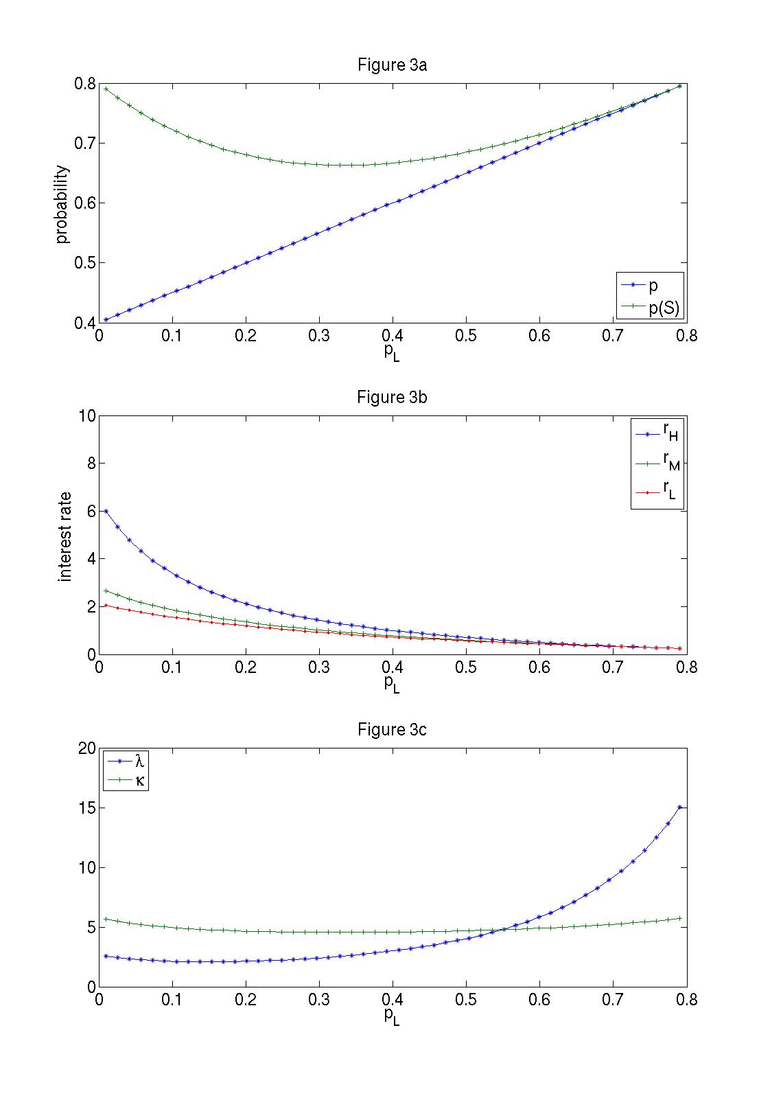
To illustrate why the outside expected rate is higher or lower than the inside expected rate, Figures 2 and 3 show cross sections of the components of Equation (7) in ![]() and
and ![]() , respectively. Figure 2 shows the change in the components across the full range of
, respectively. Figure 2 shows the change in the components across the full range of ![]() ,
holding constant the value of
,
holding constant the value of ![]() , and Figure 3 shows the same values across the full range of
, and Figure 3 shows the same values across the full range of ![]() , holding constant the value of
, holding constant the value of ![]() . In both figures, the value of theta is held constant at
. In both figures, the value of theta is held constant at ![]() . The specific numerical values for the two cross sections are chosen to illustrate the most straight forward changes in the components. The panels in Figures 2 and 3 have the following order: the 2a and 3a panels show the values of
. The specific numerical values for the two cross sections are chosen to illustrate the most straight forward changes in the components. The panels in Figures 2 and 3 have the following order: the 2a and 3a panels show the values of ![]() and
and ![]() ; the 2b and 3b panels show the values of
; the 2b and 3b panels show the values of ![]() ,
, ![]() , and
, and ![]() ; and the 2c and 3c panels show the values of
; and the 2c and 3c panels show the values of ![]() and
and ![]() ,
defined as
,
defined as
![]() and
and
![]() .
.
In Figure 2a, ![]() is linearly increasing in
is linearly increasing in ![]() at a constant rate of
at a constant rate of ![]() and
and ![]() is increasing in
is increasing in ![]() at a non-linear rate greater than
at a non-linear rate greater than ![]() . The value of
. The value of ![]() is increasing in
is increasing in ![]() because the probability of success is higher for
because the probability of success is higher for ![]() firms and the quality of the
firms and the quality of the ![]() signal is increasing (
signal is increasing (![]() is increasing relative to
is increasing relative to ![]() . Figure 2b shows that
. Figure 2b shows that ![]() and
and
![]() are both decreasing in
are both decreasing in ![]() . This is because the higher probability of success
for
. This is because the higher probability of success
for ![]() firms leads to lower rates. The value of
firms leads to lower rates. The value of ![]() is non-monotonic in
is non-monotonic in ![]() due to the non-monotonicity of
due to the non-monotonicity of ![]() in
in ![]() , which is because
, which is because ![]() has two opposing effects on
has two opposing effects on ![]() . First,
. First, ![]() has a positive effect on
has a positive effect on ![]() because
the probability of success is higher if the
because
the probability of success is higher if the ![]() signal occurs for an
signal occurs for an ![]() firm. Second,
firm. Second,
![]() has a negative effect on
has a negative effect on ![]() because the probability of
because the probability of ![]() occurring for an
occurring for an ![]() firm increases.7 In Figure 2c, both
firm increases.7 In Figure 2c, both ![]() and
and ![]() are increasing in
are increasing in ![]() , but
, but ![]() increases at a much faster rate at higher levels of
increases at a much faster rate at higher levels of ![]() . For this case of
. For this case of ![]() , the two curves cross at a value of
, the two curves cross at a value of ![]() between 0.8 and 0.85. This is precisely where the expected inside rate becomes greater than the expected outside rate, as shown
in Figure 1b.
between 0.8 and 0.85. This is precisely where the expected inside rate becomes greater than the expected outside rate, as shown
in Figure 1b.
In Figure 3a, the value of ![]() is linearly increasing in
is linearly increasing in ![]() at a constant rate of
at a constant rate of
![]() , whereas the value of
, whereas the value of ![]() is non-montonic in
is non-montonic in ![]() . The value of
. The value of ![]() is non-monotonic in
is non-monotonic in ![]() because
because ![]() has two opposing effects on
has two opposing effects on ![]() . First,
. First, ![]() has a positive effect on
has a positive effect on ![]() because the
probability of success is higher if the
because the
probability of success is higher if the ![]() signal occurs for an
signal occurs for an ![]() firm. Second,
firm. Second,
![]() has a negative effect on
has a negative effect on ![]() because the probability of
because the probability of ![]() occurring for an
occurring for an ![]() firm increases.8 In Figure 3b, the values of
firm increases.8 In Figure 3b, the values of ![]() ,
, ![]() , and
, and ![]() are all decreasing in
are all decreasing in ![]() . This is
because the higher probability of success for
. This is
because the higher probability of success for ![]() firms leads to lower rates. Figure 3c shows that the change in both
firms leads to lower rates. Figure 3c shows that the change in both ![]() and
and ![]() is non-monotonic in
is non-monotonic in ![]() , but
, but
![]() increases at a much faster rate at higher levels of
increases at a much faster rate at higher levels of ![]() . For this case of
. For this case of
![]() , the two curves cross at a value of
, the two curves cross at a value of ![]() between 0.5 and 0.6, where the
expected inside rate becomes greater than the expected outside rate, as shown in Figure 1b.
between 0.5 and 0.6, where the
expected inside rate becomes greater than the expected outside rate, as shown in Figure 1b.
The numerical results in Figures 2c and 3c show that the changes in
![]() over the parameter space are relatively small compared to the changes in
over the parameter space are relatively small compared to the changes in
![]() . Therefore, an analysis of the difference in the inside and outside expected interest rate in Proposition A can loosely be considered in terms of
. Therefore, an analysis of the difference in the inside and outside expected interest rate in Proposition A can loosely be considered in terms of ![]() and
and ![]() .9
.9
As can be seen from Equations (5) and (6), the difference between the inside and outside expected rates reflects the relative weightings of the low and high expected rate contracts in the total lending of the inside and outside bank. If ![]() is high, there is a high proportion of good firms (
is high, there is a high proportion of good firms (![]() and the outside bank is bidding from
and the outside bank is bidding from ![]() with a high probability (
with a high probability (![]() , such that there are a high proportion of low expected rate loans made by both
the inside and outside bank. The outside bank makes more
, such that there are a high proportion of low expected rate loans made by both
the inside and outside bank. The outside bank makes more ![]() loans than the inside bank, therefore the expected outside rate is higher. The outside bank wins more medium rate contracts, so
the expected outside rate is higher than the expected inside rate, making
loans than the inside bank, therefore the expected outside rate is higher. The outside bank wins more medium rate contracts, so
the expected outside rate is higher than the expected inside rate, making
![]() positive. On the other hand, if
positive. On the other hand, if ![]() is high, then the
proportion of good firms in the borrower pool (
is high, then the
proportion of good firms in the borrower pool (![]() is low and the outsider bids from
is low and the outsider bids from ![]() with a low probability (
with a low probability (![]() , so the proportion of high expected rate loans is large in both banks' lending. The outside bank makes more medium expected rate loans, so
the outside expected rate is lower than the inside expected rate, making
, so the proportion of high expected rate loans is large in both banks' lending. The outside bank makes more medium expected rate loans, so
the outside expected rate is lower than the inside expected rate, making
![]() negative.
negative.
The following interpretation of Figure 1 is based on the mappings of
![]() space into
space into ![]() space. Figure 1 shows that the outside
rate is always higher than the inside rate when
space. Figure 1 shows that the outside
rate is always higher than the inside rate when ![]() and
and ![]() are sufficiently high.
In all three panels, as
are sufficiently high.
In all three panels, as ![]() and
and ![]() , the outside rate is higher than
the inside rate, independent of
, the outside rate is higher than
the inside rate, independent of ![]() .10 This is
where
.10 This is
where ![]() and
and ![]() . The result confirms that the expected outside rate is
higher than the expected inside rate when
. The result confirms that the expected outside rate is
higher than the expected inside rate when ![]() and
and ![]() are sufficiently high. In the
lower left corner of the parameter space of Figure 1, where
are sufficiently high. In the
lower left corner of the parameter space of Figure 1, where ![]() and
and ![]() are both
low, the inside expected rate is higher than the outside expected rate. This is where
are both
low, the inside expected rate is higher than the outside expected rate. This is where ![]() and
and ![]() are low, which shows that the inside expected rate is higher than the outside rate when
are low, which shows that the inside expected rate is higher than the outside rate when ![]() and
and ![]() are sufficiently low.
are sufficiently low.
The panels of Figure 1 also indicate that the difference in the inside and outside expected rates depends on ![]() . This is especially true in the corner of
. This is especially true in the corner of ![]() space where
space where ![]() is high and
is high and ![]() is low. In this corner, when
is low. In this corner, when ![]() is low, the expected inside rate is higher than the expected outside rate, and when
is low, the expected inside rate is higher than the expected outside rate, and when ![]() is high, the expected outside rate is higher than the expected inside rate. This result makes sense in light of the values of
is high, the expected outside rate is higher than the expected inside rate. This result makes sense in light of the values of ![]() and
and ![]() , given these parameter values. When
, given these parameter values. When ![]() is high and
is high and
![]() is low, the value of
is low, the value of ![]() depends heavily on the value of
depends heavily on the value of ![]() whereas
whereas ![]() is less sensitive to
is less sensitive to ![]() . When
. When ![]() is low,
is low, ![]() is low in this corner, and when
is low in this corner, and when ![]() is high,
is high, ![]() is high in this corner. This is
because a low
is high in this corner. This is
because a low ![]() weights
weights ![]() toward
toward ![]() and a high
and a high ![]() weights
weights ![]() toward
toward ![]() . In other words, the proportion of good firms,
. In other words, the proportion of good firms, ![]() , largely
corresponds to the value of
, largely
corresponds to the value of ![]() in this corner. When
in this corner. When ![]() is low, the proportion
of good firms is low, and the inside bank has a larger proportion of
is low, the proportion
of good firms is low, and the inside bank has a larger proportion of ![]() loans. When
loans. When ![]() is high, the proportion of good firms is high, and the inside bank has a larger proportion of
is high, the proportion of good firms is high, and the inside bank has a larger proportion of ![]() loans. Therefore, the inside rate is higher than the outside rate when
loans. Therefore, the inside rate is higher than the outside rate when
![]() is low, but the outside rate is higher than the inside rate when
is low, but the outside rate is higher than the inside rate when ![]() is
high.11
is
high.11
These results show that the outside expected rate is not always higher than the inside expected rate, as might seem to be the intuition of the winner's curse. The outside expected rate is higher than the inside expected rate when there is a high proportion of good firms in the borrower pool and
the outside bank bids below ![]() with a high probability. The inside bank wins mostly good firms at the low expected rate and the outside bank expected rate is driven up by the outside bank
offering some bad firms a rate below
with a high probability. The inside bank wins mostly good firms at the low expected rate and the outside bank expected rate is driven up by the outside bank
offering some bad firms a rate below ![]() . On the other hand, the inside expected rate is higher than the outside expected rate when there is a low proportion of good firms in the borrower
pool and the outside bank bids below
. On the other hand, the inside expected rate is higher than the outside expected rate when there is a low proportion of good firms in the borrower
pool and the outside bank bids below ![]() with some probability. In this case, the inside bank rate is high because it lends mostly to bad firms at the high rate. The outside rate is reduced
below the inside rate, because the outside bank makes low rate offers to some bad firms.
with some probability. In this case, the inside bank rate is high because it lends mostly to bad firms at the high rate. The outside rate is reduced
below the inside rate, because the outside bank makes low rate offers to some bad firms.
8. Conclusion
This paper analyzes the predictions of a benchmark model for insider vs. outsider expected interest rates. The Sharpe model (with the von Thadden correction) is a standard framework for analyzing the role of private information in the competition between bank lenders. The results of this paper show that the Sharpe model does not provide a universal prediction for inside vs. outside expected interest rates. The prediction of the model depends on the parameters of the model, which are the borrower characteristics.
There is a clear winner's curse problem for the outside bank. The outside bank wins more bad firms and less good firms than the inside bank, suggesting the intuition that the expected interest rate at the outside bank is always higher than the expected interest rate at the inside bank. The reasoning would be that outside banks win more bad firms, bad firms borrow at a higher rate, and, hence, the outside rate is higher. The interesting result of this paper is that the apparent intuition of the winner's curse leading to this conclusion does not necessarily follow. Although the outside bank wins more bad firms than the inside bank, the winner's curse also causes the expected rate for each firm type to be lower at the outside bank. In other words, conditional on firm type, firms pay a lower rate at the outside bank. When this result is combined with the effect of the winner's curse on winning bids, it becomes apparent that deriving the prediction for the expected interest rate at an insider vs. outsider requires further analysis.
The results of this paper should help refine future theoretical work on observed price outcomes in games with information asymmetries among bidders as well as future empirical work on switching. The analytical results show that the predictions of the model for expected interest rates depend on the parameters of the model, which are the borrower characteristics. To illustrate these conditions, the numerical results show that the outside expected rate is higher than the inside expected rate when the quality of the borrower pool is high and the inside rate is higher than the outside rate when the quality of the borrower pool is low. This is an important step forward in clarifying the predictions of the model for observed interest rates when firms borrow from inside vs. outside lenders.
References
Black, L., 2008. The role of relationships in mitigating information asymmetries between lenders. Working paper, Board of Governors of the Federal Reserve System.
Degryse, H., Van Cayseele, P., 2000. Relationship lending within a bank-based system: Evidence from European small business data. Journal of Financial Intermediation 9, 90-109.
Rajan, R., 1992. Insiders and outsiders: the choice between informed and arm's length debt. Journal of Finance 47, 1367-1400.
Sharpe, S., 1990. Asymmetric information, bank lending and implicit contracts: A stylized model of customer relationships. Journal of Finance 45, 1069-1087.
von Thadden, E.-L., 2004. Asymmetric information, bank lending and implicit contracts: the winner's curse. Finance Research Letters 1, 11-23.
Footnotes
In each panel, the dark area is the region in ![]() space where
space where
![]() , and the light area is the region in
, and the light area is the region in ![]() space where
space where
![]() .
.
![Figure 2 has three panels and, for each panel, the X axis shows the probability of project success for H firms (pH) on the interval [0.5, 1]. All three panels show the results where pL equals 0.5 and theta equals 0.5. For Figure 2a, the Y axis displays the probability of p and p(S). For Figure 2b, the Y axis displays the interest rate of rH, rM, and rL. For Figure 2c, the Y axis displays the values of lambda and kappa. Each data point listed below is a Y-axis value of an increment of 0.2 on the X axis.](img109.gif)
>