Imperfect Information and Monetary Models:
Multiple Shocks and their Consequences
Keywords: Imperfect information, price puzzle, inflation inertia
Abstract:
JEL Codes: E31
1 Introduction
This paper incorporates multiple aggregate shocks into monetary models with imperfect information. After a contractionary monetary shock these models exhibit: a) an initial increase in inflation, i.e. the "price puzzle"; and b) a delayed disinflation, i.e. a "hump". These patterns are found in many empirical studies, for example see (Christiano et al., 2005). With multiple aggregate shocks, imperfect information implies that agents are not only unsure of the magnitude of the aggregate shock, but they are also unsure which shock has hit. In the New Keynesian variant of the models I present, when a contractionary monetary shock occurs agents see the interest rate increasing. They conclude that this is either due to a monetary disturbance or due to rising inflationary pressures, and so put some weight on both of these explanations. The weight they place on the "inflationary pressures" explanation then acts as a force inducing firms to increase their price. As time passes agents are better able to determine what has happened and start to cut prices in response to falling demand, generating a hump. I generate this pattern with very conservative parameter values.
It is important to explain what happens after a monetary shock because it influences how we view the monetary transmission mechanism and its associated delays. Empirically, the existence of the price puzzle is contentious. In vector autoregression exercises it is often suggested that augmentation of models with commodity prices eliminates the problem, see for example (Christiano et al., 1999). (Hanson, 2004) argued that this is most likely a coincidence. Hanson also pointed that out that some authors have proposed informal specification tests where a model is rejected if the price puzzle is found. Such specification tests are flawed if the price puzzle is indeed a structural part of the economy. By contrast the existence of the hump is widely accepted (eg. (Romer & Romer, 2004), (Bernanke et al., 2005)) but how it is modeled often lacks microfoundations. Typically it is achieved by assuming some sort of indexing behavior (see (Woodford, 2003b)).
In addition, I show that increased price flexibility can lead to more monetary non-neutrality. This runs counter to the results of traditional models, where the very source of non-neutrality is price stickiness. The recent controversy over the degree of stickiness in the United States ((Bils & Klenow, 2004), (Nakamura & Steinsson, Forthcoming)) has certainly been viewed through this conventional prism. The findings in this paper question that presumption.
Monetary models with imperfect information have experienced a revival of late. Initially they were popularized by (Lucas, 1972), who expanded upon some ideas of (Friedman, 1968) and (Phelps, 1969), but their use waned after
the 70s. (Woodford, 2003a) noted that this was, at least partially, because the simplifying assumptions needed to solve the models implied short-lived fluctuations. For example (Lucas, 1972) assumed everything became common knowledge after one
period's duration. However (Woodford, 2003a) was able to get around such problems, obtaining long-lived responses to shocks. This, along with Sims's work on rational inattention ((Sims, 2003)), sparked much of the revival. One notable characteristic
of this new work is the introduction of situations where agents have different information sets. This can introduce higher order expectations into models, where agents' actions depend upon what they believe other agents believe. This was the crucial mechanism in (Woodford,
2003a). Other topics have been investigated in this literature. For example (Ma![]() kowiak & Wiederholt, Forthcoming) looked at how agents allocate their attention between aggregate and
idiosyncratic shocks. (Gorodnichenko, 2008) analyzed a menu cost model where information gets "trapped" when firms do not reset their price. I have a different focus. Uncertainty regarding which aggregate shocks have hit the economy drives the results. It also illustrates a
broader methodological point. In imperfect information models all significant aggregate shocks should be included in order to get accurate model predictions.
kowiak & Wiederholt, Forthcoming) looked at how agents allocate their attention between aggregate and
idiosyncratic shocks. (Gorodnichenko, 2008) analyzed a menu cost model where information gets "trapped" when firms do not reset their price. I have a different focus. Uncertainty regarding which aggregate shocks have hit the economy drives the results. It also illustrates a
broader methodological point. In imperfect information models all significant aggregate shocks should be included in order to get accurate model predictions.
The paper proceeds as follows. Section 2 introduces a simple static model that demonstrates some of the main points of the paper. Section 3, introduces imperfect information into a traditional New Keynesian framework. Sharply different results are generated than would be the case if information were perfect, even though agents are very good at determining what is occurring. Section 4 considers the stabilizing role of sticky prices, showing that greater flexibility can induce more volatility. Section 5 concludes.
2 Simple Static Model
The model presented in this section is static and hence cannot replicate the delayed disinflation. However, it is usually the case that anything that enhances the price puzzle enhances the hump in the model of Section 3. Therefore I view the static exercise as
informative. There are a continuum of firms, indexed by ![]() on the interval
on the interval ![]() . A
firm's price is a positive function of their expectation of the aggregate price level, the level of economic activity, and a common markup shock. Formally, each firm sets the log of their price according to the following rule:
. A
firm's price is a positive function of their expectation of the aggregate price level, the level of economic activity, and a common markup shock. Formally, each firm sets the log of their price according to the following rule:
Monetary policy is conducted in the form of a money supply rule. Because the central bank dislikes the inflationary consequences of markup shocks, the money supply is cut when they occur. The money supply is also subject to its own shocks. Explicitly:

The two shocks that hit the economy, ![]() and
and ![]() , are uncorrelated and normally
distributed:
, are uncorrelated and normally
distributed:
![\displaystyle X=\left[ \begin{array}{c} \psi\ \nu \end{array} \right]\sim N(0,\Sigma)](img15.gif)
![\displaystyle \Sigma=\left[ \begin{array}{cc} \sigma_{\psi}^{2} & 0\ 0 & \sigma_{\nu}^{2}\end{array} \right]](img16.gif)
Each firm receives an idiosyncratic noisy signal, ![]() , of the money supply,
, of the money supply, ![]() ,
and markup shock,
,
and markup shock, ![]() , where the noise associated with each observation is normally distributed and uncorrelated with the other, i.e.:
, where the noise associated with each observation is normally distributed and uncorrelated with the other, i.e.:
![\displaystyle B=\left[ \begin{array}{cc} 1 & -\frac{1}{\phi}\ 0 & 1 \end{array} \right]](img20.gif)
![\displaystyle \mu\sim N(0,\Sigma_{n}),\ \Sigma_{n}=\left[ \begin{array}{cc} \sigma_{n,m}^{2} & 0\ 0 & \sigma_{n,\nu}^{2}\end{array} \right]](img21.gif)
Agents also know the parameters of the model and all firms have rational expectations, so:

-
 are rational
 - Given
 ,
,
 , and
, and

-

 where
where

Appendix A shows that the equilibrium is unique. If the price level after a monetary shock is considered, the following results are obtained:

-

 if
if
 where
where

The first result,
This mechanism relies on agents using their signal of the central bank's action to update their beliefs. This would imply that the central bank has some separate information that the public does not posses. This information structure finds empirical support in the study of (Romer & Romer, 2000), who conclude that "the Federal Reserve has considerable information about inflation beyond what is known to commercial forecasters".
If the variance of the markup shock is increased then firms will attribute more of what they see to a markup shock. Therefore firms will set a higher price than they otherwise would, which explains why
![]() . Indeed, the confusion about which shock has occurred can be so severe that prices may go up after a contractionary
monetary shock. This price puzzle result occurs if
. Indeed, the confusion about which shock has occurred can be so severe that prices may go up after a contractionary
monetary shock. This price puzzle result occurs if
![]() , i.e. if the relative variance of the monetary shocks is sufficiently small.
, i.e. if the relative variance of the monetary shocks is sufficiently small.
3 A New Keynesian Model
The model above abstracts from many different issues. For example, central banks rarely use money supply as a policy instrument. Also, in the model firms get signals of exogenous variables, ![]() and
and ![]() , and not endogenous variables such as prices,
, and not endogenous variables such as prices, ![]() . I address
these and other issues in the more sophisticated model that follows.
. I address
these and other issues in the more sophisticated model that follows.
3.1 The Model
The core components of this model follow a standard New Keynesian model, in the tradition of (Woodford, 2003b) and (Clarida et al., 1999). The point of departure is that each agent has an idiosyncratic information set.
3.1.1 Private Agents
There are a continuum of private agents indexed by ![]() . In what follows,
. In what follows, ![]() and
and ![]() index time periods. Each agent in the economy can be thought of as a yeoman farmer, producing a unique good, also indexed by
index time periods. Each agent in the economy can be thought of as a yeoman farmer, producing a unique good, also indexed by ![]() . The only input into production is labor with functional form:
. The only input into production is labor with functional form:
Each period the agent consumes a finite number of goods, ![]() . The identity of these goods is chosen randomly from the continuum in the economy. This is intended to limit the amount of
information that the agent can infer from their consumption basket about the overall price level.2 The per period utility function of agent
. The identity of these goods is chosen randomly from the continuum in the economy. This is intended to limit the amount of
information that the agent can infer from their consumption basket about the overall price level.2 The per period utility function of agent ![]() is a linearly separable function of a consumption index and labor:
is a linearly separable function of a consumption index and labor:


The only asset in the economy is a nominal one-period bond, so the budget constraint at time ![]() is:
is:
where
for all points along a planned consumption path, where
Appendix B shows that this implies:
and:
with price index:
The agent will sell to
where
Prices are sticky using the (Calvo, 1983) specification. Specifically, there is a probability equal to ![]() that the agent will have the opportunity to reset their
price in any given period. The discount factor is
that the agent will have the opportunity to reset their
price in any given period. The discount factor is ![]() .
.
At the end of each time period, the agent observes their own
![]() ; how much they sell,
; how much they sell, ![]() ; the prices in their consumption basket,
; the prices in their consumption basket,
![]() ; and the price of the nominal bond,
; and the price of the nominal bond, ![]() . Agents get
to see these only after they have made the decision on
. Agents get
to see these only after they have made the decision on ![]() and
and
![]() .4 Therefore the information used
when making decisions on
.4 Therefore the information used
when making decisions on ![]() and
and
![]() is:
is:
However, when deciding on
As a result, using the production function, the agent's problem can be written as choosing a plan for
![]() and
and ![]() under each state of the world that maximizes:
under each state of the world that maximizes:
subject to Equations 1, 2, 6, and 7 with sticky prices à la (Calvo, 1983), where the hazard is
Agents are rational, so that the underlying probability density functions used to calculate expectations are those implied by the model.
3.1.2 The Central Bank
The easiest and most conventional characterization of monetary policy is a Taylor Rule:
where


Inflation is defined as the rate of change of the aggregate idealized price index:6
The addition of the lagged interest rate on the right hand side of Equation 9 reflects the large and significant value for ![]() found in many studies, for example
see (Clarida et al., 1998). This dependence upon past rates is usually interpreted as "interest rate smoothing".
found in many studies, for example
see (Clarida et al., 1998). This dependence upon past rates is usually interpreted as "interest rate smoothing".
3.2 Equilibrium
I now define equilibrium:
-
 are rational.
 - Each agent is randomly assigned
 consumption goods and
  customers.
 - Prices and allocations satisfy the agent's problem, i.e. Equation 8.
-
 .
.
The model is log linearized around a perfect information, zero inflation steady state (Appendix C). The solution method is described in Appendix D.
3.3 Numerical Illustration
I begin my exposition of this model with the parameter values specified in Tables 1 and 2. I will argue that these parameter values are conservative, in the sense that parameter values that lead to a larger price puzzle and a more delayed
disinflation can be justified. Table 1 covers parameter values that would affect the economy's reaction to a monetary shock even if information were perfect. A time period is specified to be a quarter, so the Calvo hazard parameter of 0.25 implies an average price duration
of a year. This accords with some older estimates, see for example (Blinder et al., 1998), but is slightly longer than some more recent work. For example, (Nakamura & Steinsson, Forthcoming) find a median duration for prices of 8-11 months. The
intertemporal elasticity of substitution is 1, following the real business cycle literature ((Woodford, 2003b), p. 165). I base the coefficients of the Taylor Rule on well known estimates (eg. (Clarida et al., 2000)). The discount factor,
![]() , is equal to 1.7 This eliminates some wealth
effects that would otherwise render the model difficult to solve, as described in Appendix C.
, is equal to 1.7 This eliminates some wealth
effects that would otherwise render the model difficult to solve, as described in Appendix C.
The parameters mentioned thus far do not affect the results significantly if varied over plausible ranges. That is not true for the last two parameters in Table 1. The steady state value of ![]() is
3/4, which corresponds to an elasticity of substitution between goods of 4. This is on the low side of existing calibrations, see for example (Chari et al.,
2000), but it is consistent with the recent empirical work of (Broda & Weinstein, 2006). The elasticity of output with respect to the labor input,
is
3/4, which corresponds to an elasticity of substitution between goods of 4. This is on the low side of existing calibrations, see for example (Chari et al.,
2000), but it is consistent with the recent empirical work of (Broda & Weinstein, 2006). The elasticity of output with respect to the labor input, ![]() , is
0.9, so the model's labor share of income is 0.6.8As pointed out in (Woodford, 2003b), strategic complementarity in pricing, i.e. the situation where an agent wishes to increase their price in response to an increase in the price of others, is increasing in
, is
0.9, so the model's labor share of income is 0.6.8As pointed out in (Woodford, 2003b), strategic complementarity in pricing, i.e. the situation where an agent wishes to increase their price in response to an increase in the price of others, is increasing in
![]() and decreasing in
and decreasing in ![]() . Therefore my values correspond to low levels
of strategic complementarity relative to other work, see again (Chari et al., 2000) and also (Rotemberg & Woodford, 1997). This is conservative in the sense that stronger strategic complementarity leads to a larger price puzzle and a longer delay in
disinflation. This is discussed in Section 3.5.
. Therefore my values correspond to low levels
of strategic complementarity relative to other work, see again (Chari et al., 2000) and also (Rotemberg & Woodford, 1997). This is conservative in the sense that stronger strategic complementarity leads to a larger price puzzle and a longer delay in
disinflation. This is discussed in Section 3.5.
Table 2 specifies parameter values that would not affect the economy's reaction to a monetary shock if information were perfect.9 I
can normalize the variance of the markup shock to 1 because ratios of variances determine agents' signal extraction calculations. The autocorrelation of ![]() is 0.95. I base this on
(Smets & Wouters, 2007). This study estimated a structural model of the US economy using Bayesian methods and found that markup shocks are extremely persistent, with an autocorrelation of at least 0.9.10
is 0.95. I base this on
(Smets & Wouters, 2007). This study estimated a structural model of the US economy using Bayesian methods and found that markup shocks are extremely persistent, with an autocorrelation of at least 0.9.10
I choose the final three parameters, namely the variance of the monetary shock, the number of goods in the consumption basket, and the variance of the idiosyncratic ![]() shock, to give
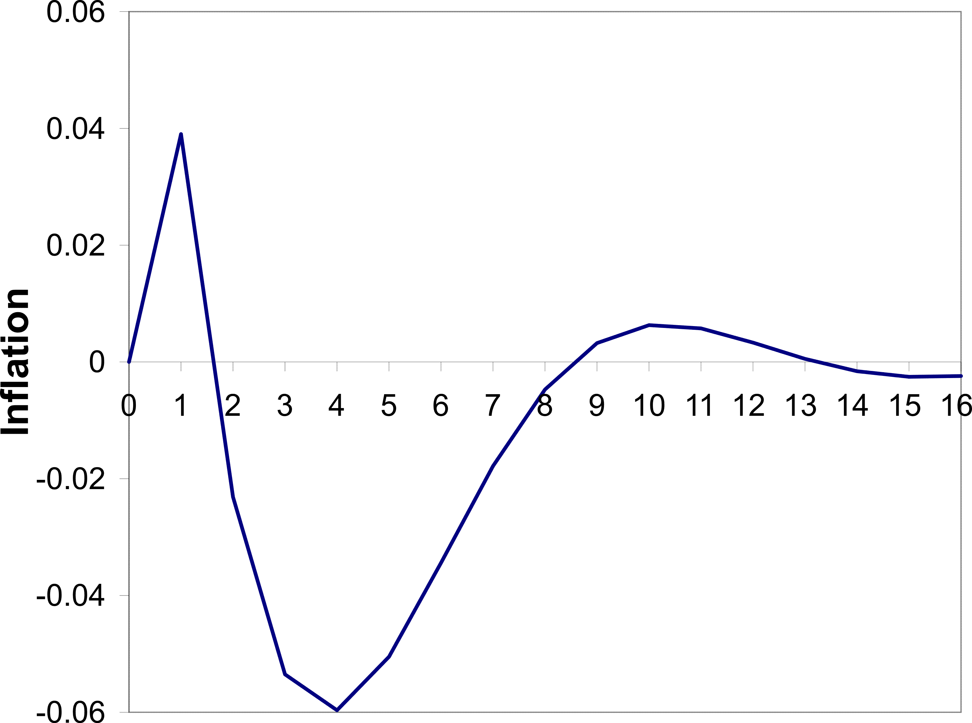
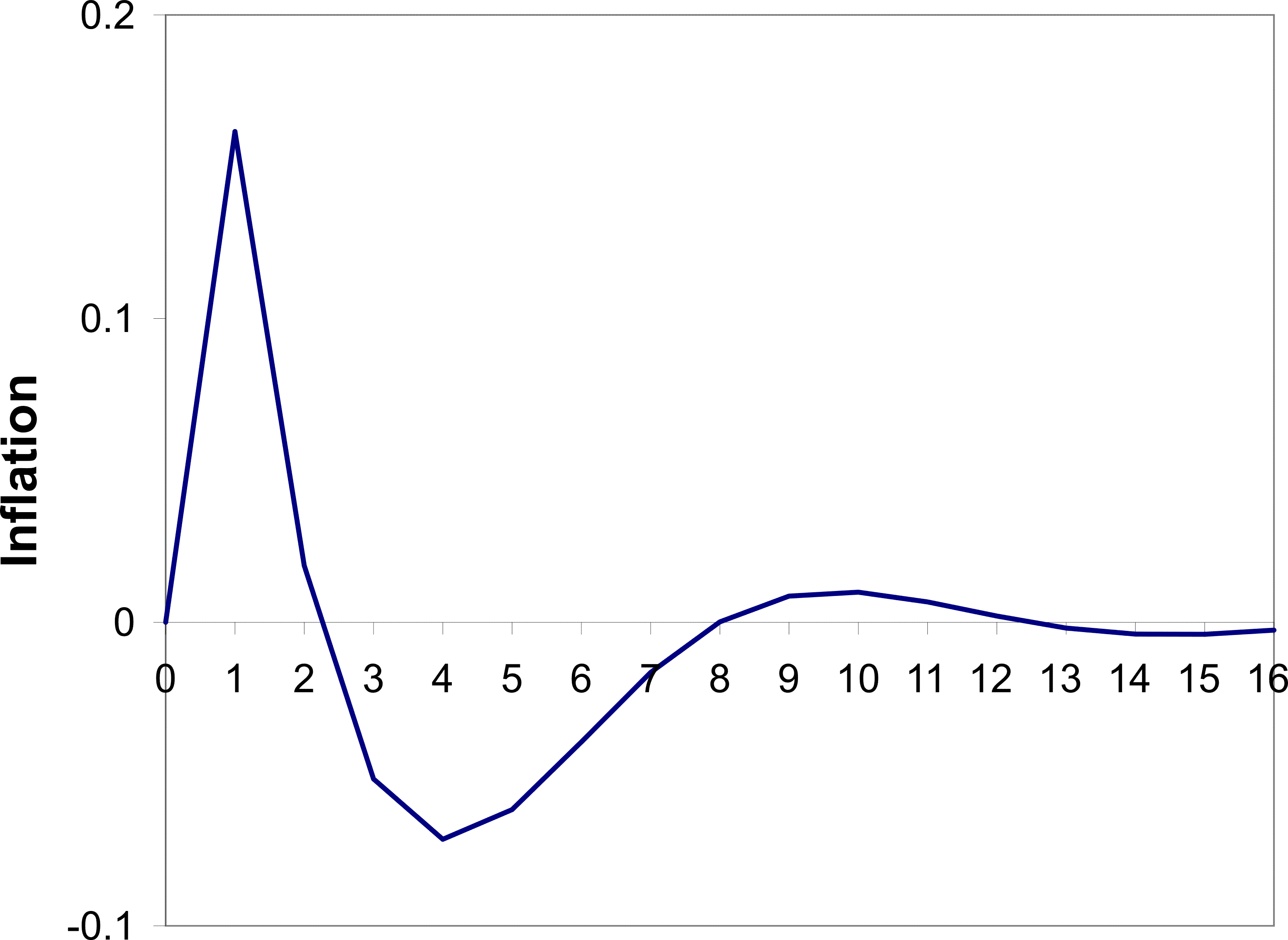
the price puzzle and a delayed disinflation. I shall discuss these parameters in Section 3.4. The resulting impulse response of inflation to a monetary shock is shown in Figure 1. By design, the inflation rate initially increases. This
increase results from the same forces discussed in Section 2. Agents see the interest rate increasing and conclude that this is partly because the central bank is responding to a positive markup shock. Agents therefore increase their price.
shock, to give
the price puzzle and a delayed disinflation. I shall discuss these parameters in Section 3.4. The resulting impulse response of inflation to a monetary shock is shown in Figure 1. By design, the inflation rate initially increases. This
increase results from the same forces discussed in Section 2. Agents see the interest rate increasing and conclude that this is partly because the central bank is responding to a positive markup shock. Agents therefore increase their price.
The period of peak disinflation occurs 4 quarters after the shock. This hump is generated by the same forces generating the price puzzle. Agents are not sure which shock has hit the economy and as a result they do not cut prices initially. As time passes they gather more information and form a better picture of the shock. They then act upon the fall in demand and begin to cut their prices. This source of the hump is different to the source in (Woodford, 2003a) and other imperfect information work, for example (Nimark, 2008). That vein of literature produces a hump through a high autocorrelation of the shock and inertia in higher order expectations-beliefs of what other agents believe. In that framework, when the shock occurs agents form an opinion about the shock, but they believe other agents are less perceptive of it. Strategic complementarity then dictates that prices will not move quickly. However, as time passes higher order expectations adjust and agents begin to change their price more aggressively. This delayed response is aided by the autocorrelation of the shock. In contrast, the mechanism I emphasize has no reliance on these higher order expectations or autocorrelation of the monetary shock.
There is also another period of inflation beginning 9 quarters after the shock. This is part of some oscillatory behavior that dies down eventually. It appears to be driven by beliefs. At that point agents are still updating their beliefs of what happened in the past, but also of what happened relatively recently. In the periods leading up to the 9 quarter mark, agents are revising their beliefs of recent markup shocks upward.
3.4 The Final Three Parameters
I now focus attention on the parameters I chose in order to generate the patterns in Figure 1, namely the variance of the monetary shock,
![]() ; the number of goods in the consumption basket,
; the number of goods in the consumption basket, ![]() ; and the variance
of the idiosyncratic
; and the variance
of the idiosyncratic ![]() shock,
shock,
![]() . While in some ways, estimating these parameters would have been desirable, computational issues rendered this impractical.
. While in some ways, estimating these parameters would have been desirable, computational issues rendered this impractical.
Section 2 demonstrated that the relative variance of the two shocks influences the price level. Table 2 specifies
![]() . I conduct a variance decomposition from simulated data as a guide to determine how this relates to the real world importance of this shock. The results are shown in
Table 3.
. I conduct a variance decomposition from simulated data as a guide to determine how this relates to the real world importance of this shock. The results are shown in
Table 3.
In the model, monetary shocks account for over half of the four period ahead output forecast error. However, such a significant role for monetary shocks has little empirical support, see for example (Kim, 1999) and (Kim & Roubini, 2000). These studies
concluded that monetary shocks are only responsible for 10-20 per cent of forecast errors. In the estimated model of (Smets & Wouters, 2007), the contribution of monetary shocks was either on the low side of this 10-20 per cent range or below it at all horizons. While the
numbers from Table 3 are in the right ballpark in the longer run, it is the short horizon figures heavily influence learning in the first few periods after the shock, and so should be emphasized. Therefore even lower values of
![]() can be justified, so in this sense
can be justified, so in this sense
![]() is conservative. However, the model has only two shocks. If other shocks were added, then to keep the numbers in Table 3 stable, the variance
of the markup shocks would have to be reduced. The rejoinder to this point is that most other major shocks that would be replacing the markup shock would induce the same sort of response. Take for example an aggregate demand shock. If added to the model, then when interest rates increase agents
will attribute this partly to rising demand, which will place upward pressure on their price. Specifications that included demand shocks have been experimented with and the qualitative features of the results are not changed.
is conservative. However, the model has only two shocks. If other shocks were added, then to keep the numbers in Table 3 stable, the variance
of the markup shocks would have to be reduced. The rejoinder to this point is that most other major shocks that would be replacing the markup shock would induce the same sort of response. Take for example an aggregate demand shock. If added to the model, then when interest rates increase agents
will attribute this partly to rising demand, which will place upward pressure on their price. Specifications that included demand shocks have been experimented with and the qualitative features of the results are not changed.
The other two parameters left to consider are
![]() and
and ![]() , i.e. the variance of the individual shock to
, i.e. the variance of the individual shock to
![]() and the number of goods consumed by each agent. These determine how well agents perceive the state of the economy because they govern the precision of their signals. While errors of
beliefs regarding the actual shocks can't be measured, errors of beliefs regarding aggregates can from the Survey of Professional Forecasters. This survey includes a question on respondents' expectations of GDP for the current quarter. Models of perfect information imply that agents should know
this exactly. Table 4 shows that they do not. The statistic used to show this is the ratio of the mean square error of the average forecast of the output gap to its variance. This is a variable that is negatively related to how well agents perceive current conditions.
This statistic is 0.186 in the data, which is more than a factor of 70 greater than the model implies. Therefore, the results are not dependent upon assuming an unrealistic degree of uncertainty. In this sense
and the number of goods consumed by each agent. These determine how well agents perceive the state of the economy because they govern the precision of their signals. While errors of
beliefs regarding the actual shocks can't be measured, errors of beliefs regarding aggregates can from the Survey of Professional Forecasters. This survey includes a question on respondents' expectations of GDP for the current quarter. Models of perfect information imply that agents should know
this exactly. Table 4 shows that they do not. The statistic used to show this is the ratio of the mean square error of the average forecast of the output gap to its variance. This is a variable that is negatively related to how well agents perceive current conditions.
This statistic is 0.186 in the data, which is more than a factor of 70 greater than the model implies. Therefore, the results are not dependent upon assuming an unrealistic degree of uncertainty. In this sense
![]() and
and ![]() are conservative.
are conservative.
3.6 Comparative Statics
I will not document the sensitivity of the results to changes in all of the parameters from Section 3.3. I shall instead focus on the most interesting cases. These are
![]() ,
, ![]() and
and
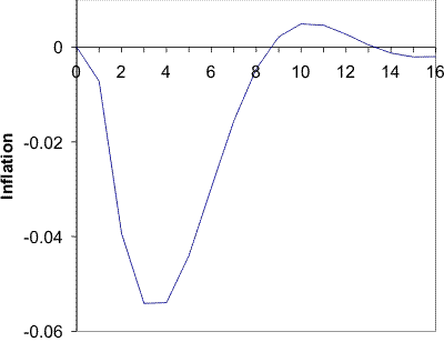
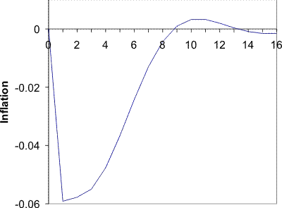
![]() . Variations in the remaining paramters over plausible values have little effect on the results. Figure 3 shows that increasing the
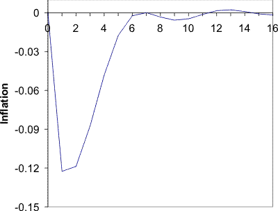
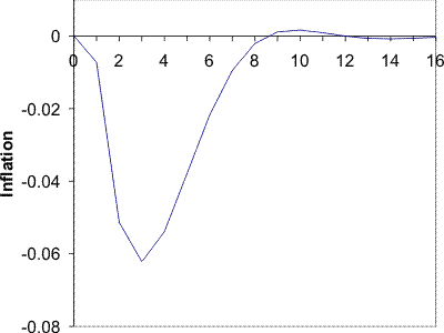
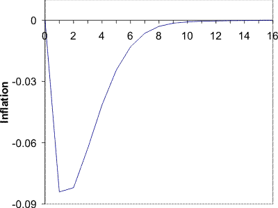
variance of the interest rate shock and increasing the precision of the signals reduces the price puzzle and brings the peak effect on inflation forward. The left panel shows values for which the price puzzle is eliminated. The right panel shows the points at which the hump is eliminated.
. Variations in the remaining paramters over plausible values have little effect on the results. Figure 3 shows that increasing the
variance of the interest rate shock and increasing the precision of the signals reduces the price puzzle and brings the peak effect on inflation forward. The left panel shows values for which the price puzzle is eliminated. The right panel shows the points at which the hump is eliminated.
Increasing
![]() from 0.07 to 0.09 eliminates the price puzzle. This increase pushes the four period ahead forecast error due to monetary shocks up from 51% to 54%. Increasing the variance
further to 0.13 eliminates the hump. In this case the forecast error due to monetary shocks is 60%.
from 0.07 to 0.09 eliminates the price puzzle. This increase pushes the four period ahead forecast error due to monetary shocks up from 51% to 54%. Increasing the variance
further to 0.13 eliminates the hump. In this case the forecast error due to monetary shocks is 60%.
Increasing ![]() and decreasing
and decreasing
![]() in integer steps eliminates the price puzzle at
in integer steps eliminates the price puzzle at ![]() and
and
![]() . These parameters correspond to ratios calculated in Table 4 of 0.0025 and 0.0023 respectively. Continuing this process means the hump
is eliminated when
. These parameters correspond to ratios calculated in Table 4 of 0.0025 and 0.0023 respectively. Continuing this process means the hump
is eliminated when ![]() and
and
![]() . These parameters correspond to a ratio calculated in Table 4 of 0.0018 and 0.0015 respectively.
. These parameters correspond to a ratio calculated in Table 4 of 0.0018 and 0.0015 respectively.
It can then be concluded that the presence of the price puzzle is quite sensitive to the parameters chosen. However, the hump is more robust.
4 Is Price Flexibility Stabilizing?
The degree of price stickiness in the United States has recently been subject to some debate. (Bils & Klenow, 2004) stimulated this debate by looking at data provided by the Bureau of Labor Statistics, arguing that the median length of price duration was a surprisingly short 4.3 months. Since this research (Nakamura & Steinsson, Forthcoming) have taken a different look at the data, generating longer estimates. This subject has received so much attention because more stickiness traditionally leads to more monetary non-neutrality. However, models have been constructed where this is not necessarily the case. For example, in a Keynesian model, (DeLong & Summers, 1986) showed that increased price flexibility can be destabilizing due to a "Mundell" effect. In their model increased price flexibility implied future prices were expected to fall further after a contractionary shock. The dependence of the forward looking IS curve on the real interest rate then dictated that agents would reduce their demand further, exacerbating the shock.
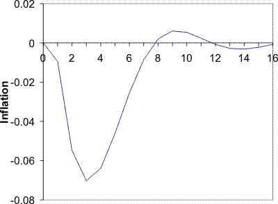
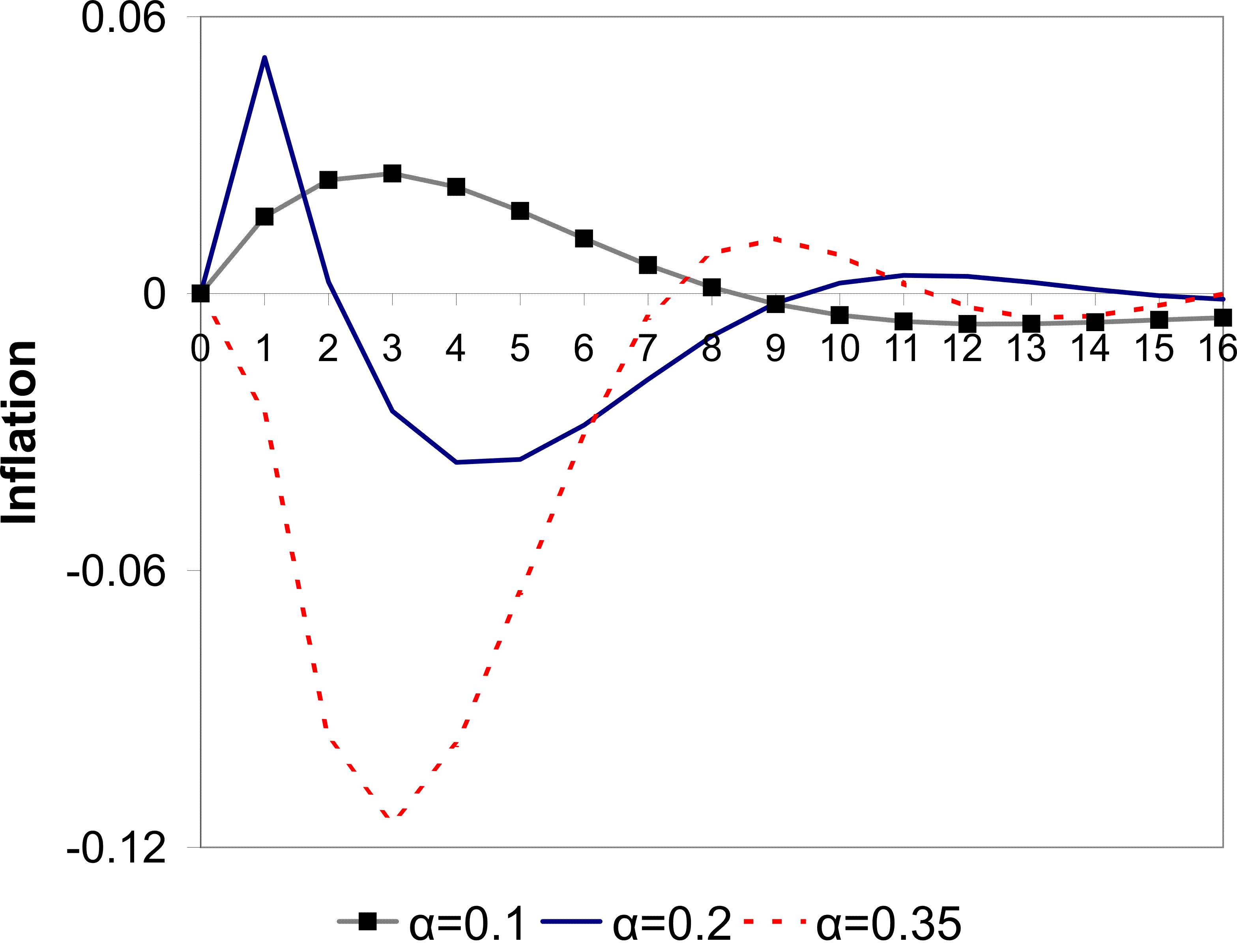
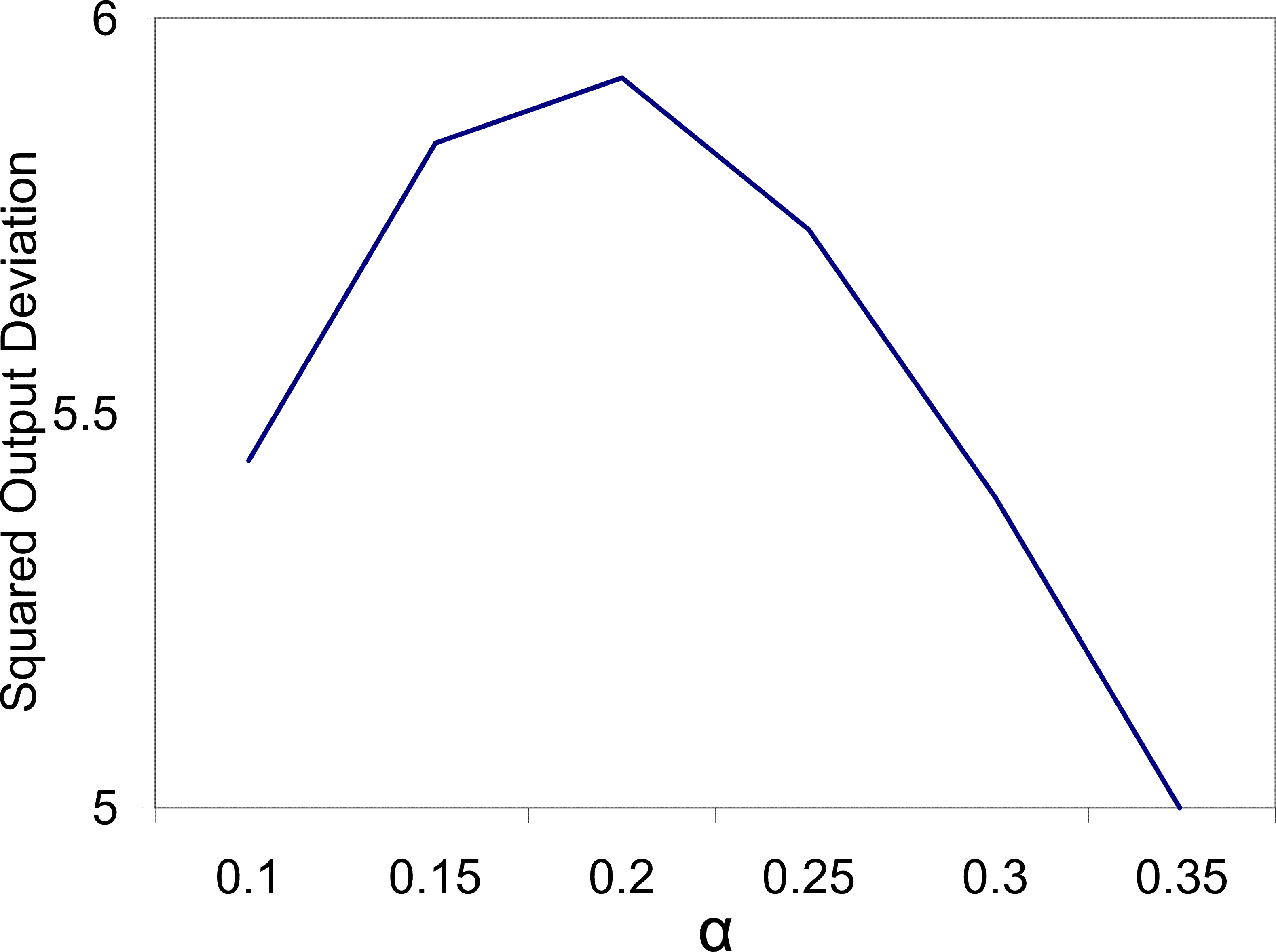
Similarly in this model, increased price flexibility can be destabilizing after a monetary shock, but for different reasons. Figure 4 shows that, with the baseline parameters from Section 3.3, output stability is increasing in
price flexibility up to the point of
![]() . The reason is simple, increased price flexibility means that the initial price puzzle is more pronounced and this destabilizes output. For price flexibility greater than
. The reason is simple, increased price flexibility means that the initial price puzzle is more pronounced and this destabilizes output. For price flexibility greater than
![]() , the initial price puzzle is mitigated when
, the initial price puzzle is mitigated when ![]() is increased. This
is because a different influence dominates pricing decisions arising from the dynamic nature of price setting. Prices in the future will be lower if price flexibility is increased. Therefore, agents' new prices will fall immediately after the shock, because they may be stuck with that price for
some time.
is increased. This
is because a different influence dominates pricing decisions arising from the dynamic nature of price setting. Prices in the future will be lower if price flexibility is increased. Therefore, agents' new prices will fall immediately after the shock, because they may be stuck with that price for
some time.
It should be noted however, that the price puzzle is not a necessary precondition for a positive relationship between price flexibility and output. There are other parameterizations where an initial fall in prices is tempered with greater price flexibility, which in turn leads to more output instability. The dominant force driving this comparative static is that flexibility leads to higher prices after a positive markup shock. In equilibrium, this means that more of the variability of prices and therefore interest rates is driven by markup shocks. This leads agents to place more weight on their markup shock beliefs after a monetary shock, which acts as a force tempering the initial price decrease.
5 Conclusion
This paper presented models where agents mistook a contractionary monetary shock for the endogenous response of monetary policy. As a result, they initially increase their own price, and by more if strategic complementarity in pricing is larger. However, the models illustrate a much broader point. Imperfect information models require a complete description of the important shocks that buffet the economy in order to get accurate model predictions. Agents don't know which shock has hit the economy and therefore will attribute some of what they see to all possible disturbances. This can have large effects and serves as a note of caution for further work.
The paper has shown that the mechanism that generates the price puzzle can also generate a hump in inflation's response to a monetary shock. Hump-shaped impulse responses turn up in many places in macroeconomics, presenting theoretical challenges. Indeed, the hump-shaped impulse response is what motivated (Woodford, 2003a). The mechanism creating the hump in Figure 3 is qualitatively distinct from any that the author has seen before. While (Woodford, 2003a) had a simple model that shared some features in common with the model employed here, the explanation for the hump is different.
The New Keynesian model developed could be enhanced further in order to investigate other challenges presented by the empirical literature. A potential finding of interest is the hump-shaped response of output to monetary shocks. While the model as it stands cannot replicate this, there are modifications that can. For example, if the interest rate shock is serially correlated, then hump-shaped responses are possible.
A. Proof of Claim 1
Let ![]() denote the probability density function of
denote the probability density function of ![]() given
given
![]() . It is easy to show that
. It is easy to show that
![]() is symmetric around
is symmetric around
![]() , so
, so
Therefore integrating over all individual prices,
![\displaystyle \Rightarrow p=\int_{0}^{1}p_{j}=[\begin{array}{cc}1& 1\end{array}] B(B'\Sigma_{n}^{-1}B+\Sigma^{-1})^{-1}B'\Sigma_{n}^{-1}BX](img137.gif) |
As a result
where:


B. Derivation of Equation 3
If ![]() is taken as given then the Lagrangian for the problem is:
is taken as given then the Lagrangian for the problem is:


and:
Dividing Equation 13 by Equation 14 and rearranging gives:

C. Log-linearized first order conditions for the private agent
Substituting in Equation 6 and Equation 4, the Lagrangian is:13

where:
The first order condition with respect to ![]() yields:
yields:
where
The first order condition with respect to ![]() gives the following:
gives the following:
where
Equation 5 implies:

where
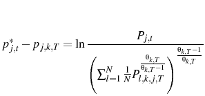
From this point I look at the solution as


D..1 The initial guess of impulse responses
Denote the initial guess for the impulse response as ![]() , a
, a ![]() matrix.15 Each column is the impulse response of a variable for the first
matrix.15 Each column is the impulse response of a variable for the first ![]() periods to one of the shocks. It is assumed that the impulse response is flat after
periods to one of the shocks. It is assumed that the impulse response is flat after ![]() periods. Let the first two columns of
periods. Let the first two columns of ![]() be the response of output (which equals consumption) to a
be the response of output (which equals consumption) to a
![]() shock and an interest rate shock. Let the following 2 columns be the response of price, then the next 2 be the response of interest rates and the next 2 the response of the
preference parameter
shock and an interest rate shock. Let the following 2 columns be the response of price, then the next 2 be the response of interest rates and the next 2 the response of the
preference parameter
![]() .
.
D..2 The state space
The true state space of the economy is postulated to be:
![\displaystyle \tilde{X}_{t}=\left[ \begin{array}{cc} \nu_{\theta,t} & \nu_{i,t}\ \nu_{\theta,t-1} & \nu_{i,t-1}\ \vdots & \vdots\\ \end{array} \right]](img195.gif)
Where
where
D..3 What is observed
From Equation 7, the following variables are used to update an agent's beliefs before making their decisions (converting these observations into their log linear counterparts):
Log linearizing Equation 6 around steady state gives:


As a result, if ![]() is defined to be:
is defined to be:
![\displaystyle \bar{M}=\left[ \begin{array}{cccc} M(1) & M(3) & M(5) & M(7) \ M(2) & M(4) & M(6) & M(8) \end{array} \right]](img226.gif)
![\displaystyle B=\left[ \begin{array}{cccc} 1 & -\frac{1}{\theta_{ss}-1}\frac{N-1}{N} & 0 & 0 \ 0 & 1 & 0 & 0 \ 0 & 0 & 1 & 0 \ 0 & 0 & 0 & 1\\ \end{array} \right]](img230.gif)
![\displaystyle \sigma_{\eta}^{2}=\left[ \begin{array}{cccc} \frac{1}{N}\sigma^{2}_{c}+(\frac{1}{1-\theta_{ss}})^{2}\frac{N-1}{N^{3}}\sigma^{2}_{p} & 0 & 0 & 0\ 0 &\frac{1}{N}\sigma^{2}_{p} & 0 & 0\ 0 & 0 &0 & 0\ 0 & 0 & 0 & \sigma^{2}_{\nu,\theta} \end{array} \right]](img232.gif)
If this is the start of the recursion, any values of
![]() and
and
![]() can be assumed. If it is not, denote previous mean square error matrix used in the Kalman filter as
can be assumed. If it is not, denote previous mean square error matrix used in the Kalman filter as ![]() . In the algorithm, calculations were made for the mean beliefs of the population for the state space. Therefore the mean square error matrix can be calculated for average beliefs, denoted
. In the algorithm, calculations were made for the mean beliefs of the population for the state space. Therefore the mean square error matrix can be calculated for average beliefs, denoted
![]() . Let
. Let
![]() be the average expectation of the state space
be the average expectation of the state space ![]() . It is easy to
show:
. It is easy to
show:

where:18
![\displaystyle \phi=-\sigma \left[ \begin{array}{cccc} 0 & 1 & 1 & 0 \end{array} \right]\bar{M}+\sigma \left[ \begin{array}{cccc} 0 & 1 & 0 & 0 \end{array} \right]\bar{M}F,\ \Phi=\phi\sum_{s=0}^{\infty} F^{s}](img246.gif)
Price setters' optimal behavior is given by Equation 20. This can be written in the form
where
D..4 Proof that the aggregate economy follows the same path as that chosen by an agent that observes no noise
Beliefs are determined by the Kalman filter19 so:
where
For the agent that observes no noise,
D..5 Calculating a new impulse response function
From the result of Appendix D.4 only the stand in agent who observes no noise needs to be considered. I first consider an interest rate shock. For the period after the shock the stand in agent has seen all variables at their baseline level in the past (which was zero) and observes:
where the last term is given by Equation 24 for the stand in agent. This follows from Appendix E. The new value for the interest rate will be given by Equation 9.
This process is then repeated for the next ![]() periods and all shocks. This is the mapping that takes us from
periods and all shocks. This is the mapping that takes us from ![]() to the new impulse response
to the new impulse response ![]() , and is iterated until convergence. Sometimes to prevent destabilizing oscillations partial adjustment is required.
, and is iterated until convergence. Sometimes to prevent destabilizing oscillations partial adjustment is required.
The adequacy of the state space postulated in Appendix D.2 is proven as Equations 23 and 24 are lienar functions of the postulated state space.
D..6 Proof that the fixed point is an equilibrium
Points 2 and 4 from the definition are trivially true because they are used in the construction at each iteration. Point 1 follows from the use of the Kalman filter by the agents, and that the actual motion of the economy follows the aggregate that the agents choose as a result of the fixed point of the iterative procedure. Point 3 follows because the new impulse responses are constructed using the solution to this problem at each iteration.
E. Evolution of the aggregate price level
The price index, ![]() , used to compute the inflation in Equation 10 is can be transformed to yield
, used to compute the inflation in Equation 10 is can be transformed to yield
where
 because the agents that get to reset their prices are chosen
randomly. Therefore Equation 28 becomes
 |
(27) |
If we approximate around the point where,

Bibliography
Federal Reserve Bank of Atlanta Economic Review 88(2):17-31.
Quarterly Journal of Economics 120(1):387-422.
Journal of Political Economy 112(5):947-985.
Russell Sage Foundation, New York.
Quarterly Journal of Economics 121(2):541-585.
Journal of Monetary Economics 12:383-398.
Econometrica 68(5):1151-1179.
In J. B. Taylor & M. Woodford (eds.), Handbook of Macroeconomics, vol. 1A. Elsevier, Amsterdam.
Journal of Political Economy 113(1):1-45.
European Economic Review 42:1033-1067.
Journal of Economic Literature 37(4):1661-1707.
Quarterly Journal of Economics 115(1):147-180.
Quarterly Journal of Economics 103(3):441-463.
American Economic Review 76(5):1031-1044.
American Economic Review 58(1):1-17.
http://www.econ.berkeley.edu/ ygorodni/gorodnichenko-endo-info-menu.pdf.
Journal Of Monetary Economics 51(7):1385-1413.
Journal of International Economics 48(2):387-412.
Journal of Monetary Economics 45(3):561-586.
Journal of Mathematical Analysis and Applications 10(2):354-367.
http://econ-www.mit.edu/files/2388.
Journal of Economic Theory 4:103-124.
American Economic Review .
Quarterly Journal of Economics .
Journal of Monetary Economics55(2).
American Economic Review 59(2):147-160.
American Economic Review 90(3):429-457.
American Economic Review 94(4):1055-1084.
NBER Macroeconomics Annual 12:297-346.
Journal of Monetary Economics 50(3):665-690.
http://sims.princeton.edu/yftpb/Macro2004/rlg.pdf.
http://sims.princeton.edu/yftp/Macro2004/Lecture1.pdf.
http://sims.princeton.edu/yftp/Macro2004/Lect2RBCStyle.pdf.
American Economic Review 97(3):586-606.
In P. Aghion, R. Frydman, J. Stiglitz, & M. Woodford (eds.), Knowledge, Information, and Expectations in Modern Macroeconomics: In Honor of Edmund S. Phelps. Princeton University Press, Princeton, NJ.
Princeton University Press, Princeton, NJ.
In J. H. Stock & M. W. Watson (eds.), Business Cycles, Indicators, and Forecasting, pp. 11-84. The University of Chicago Press, Chicago.
| Parameter | Symbol | Value |
|---|---|---|
| Calvo hazard parameter | 0.25 | |
| Int. elasticity of substitution | 1 | |
| Taylor Rule inflation coeff. |
|
1.5 |
| Taylor Rule output gap coeff. | 0.125 | |
| Interest rate smoothing | 0.7 | |
| Discount Factor | 1 | |
| Steady state |
|
3/4 |
| Elasticity of |
0.9 |
| Parameter | Symbol | Value |
|---|---|---|
| Markup shock variance |
|
1 |
|
|
0.95 | |
| Policy shock variance |
|
0.07 |
| Variance of individual |
|
7 |
| Number of goods consumed | 4 |
| 4 periods | 8 periods | 16 periods |
|---|---|---|
| 51% | 22% | 17% |
| (36,71) | (11,38) | (6,35) |
 |
sigma_i^2=0.09
sigma_i^2=0.13
N=5
N=12
sigma_mu,theta^2=3
sigma_mu,theta^2=1
|
Figure 4 B: Changes in Price Flexibility
|
Footnotes
 Return to Text


![\displaystyle E_{t}\left(\sum_{T=t}^{\infty}\beta^{T}\left[\frac{\mathcal{C}_{j,T}^{1-\sigma}}{1-\sigma}-(Y_{j,T})^{\frac{1}{\gamma}}\right]\vert I_{j,t}\right)](img77.gif)


![\begin{multline} -E_{t\vert s\in\Omega}\sum_{T=t}^{\infty}\frac{(\beta(1-\alpha... ...,T}}{\theta_{k,T}-1}}\frac{d\mathcal{P}_{k,T}}{d P_{j,t}}\right] \end{multline}](img164.gif)
![\begin{multline} E_{t\vert s\in\Omega}\Biggl[\sum_{T=t}^{\infty}(\beta(1-\alpha)... ...ta_{ss}-1}\left(p^{*}_{j,t}-p_{j,k,T}\right)\right)\Biggr)\Biggr] \end{multline}](img168.gif)


![\displaystyle X_{t}=\left[ \begin{array}{c} \nu_{\theta,t} \\ \nu_{\theta,t-1} \\ \vdots \\ \upsilon_{\theta,t}\\ \nu_{i,t} \\ \nu_{i,t-1} \\ \vdots \\ \upsilon_{i,t}\end{array} \right]](img196.gif)


