
Capital Goods Trade and Economic Development
Abstract:
1 Introduction
Cross-country differences in income per worker are large: the income per worker in the top decile is more than 40 times the income per worker in the bottom decile (Penn World Tables version 6.3, see (Heston, Summers, and Aten, 2009). Development accounting exercises such as Caselli (2005), Hall and Jones (1999), and Klenow and Rodriguez-Clare (1997) show that approximately 50 percent of the differences in income per worker are accounted for by factors of production, i.e., capital and labor, and the rest is attributed to aggregate total factor productivity (TFP).
In this paper, we argue that international trade in capital goods has quantitatively important effects on cross-country income differences through two channels: capital formation and aggregate TFP. Two facts motivate our argument: (i) capital goods production is concentrated in a few countries and (ii) the dependence on capital goods imports is systematically related to a country's level of income. The first fact is illustrated in Figure 1. Eight countries account for almost 80 percent of world capital goods production (see Eaton and Kortum (2001); capital goods production is more concentrated than GDP. The second fact is that the imports to production ratio for capital goods is negatively correlated with economic development: the correlation between the ratio and income per worker is -0.34. Malawi imports 39 times as much capital goods as it produces, Argentina imports 19 times as much as it produces, while the U.S. imports only half as much as it produces. Both facts suggest that closed economy models of capital formation can at best be only part of the explanation for cross-country factor differences.
Aggregate TFP differences across countries are also one of the consequences of international trade. Barriers to trade result in countries producing goods for which they do not have a comparative advantage. Poor countries, for instance, do not have a comparative advantage in producing capital goods, but produce too much capital goods, relative to non-capital goods. This results in a misallocation of resources and affects aggregate TFP.1 A reduction in barriers would then imply that each country specializes more in the direction of its comparative advantage resulting in a reduction in cross-country TFP differences.
We develop a multi-country Ricardian trade model along the lines of (Dornbuschm, Fischer and Samuelson (1977), Eaton and Kortum (2002), Alvarez and Lucas (2007), and Waugh (2010). Each country is endowed with labor that is not mobile internationally. Each country has technologies for producing a final consumption good, structures, a continuum of capital goods,
This figure is for our sample of 84 countries in 2005. The capital goods production data are from INDSTAT4, a database maintained by UNIDO (2010)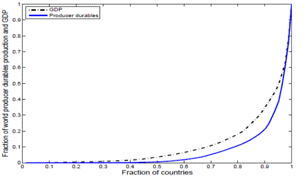
We calibrate the model to be consistent with the observed pattern of bilateral trade in capital goods and in intermediate goods, the observed relative prices of capital goods and intermediate goods (relative to final goods), and income per worker. Our model fits the trade data well: the correlation in home trade shares between the model and the data is 0.97 for capital goods and is 0.94 for intermediate goods.
Our model accounts for the fact that a few countries produce most of the capital goods in the world. The pattern of comparative advantage in our model is such that poor countries are net importers of capital goods and net exporters of intermediate goods. The average productivity gap in the capital goods sector between countries in the top and bottom deciles is almost twice as large as the gap in the intermediate goods sector.
We quantify the misallocation of resources due to trade barriers by comparing our calibrated model to a model with no trade barriers in which the allocations are optimal. Relative to the optimal allocation, countries with comparative disadvantage in the production of capital goods allocate more resources to the capital goods sector in the benchmark model. For instance, in the benchmark model, Panama allocates nearly 90 times the optimal amount of labor to the capital goods sector whereas France allocates only three-quarters of the optimal amount. With free trade the income per worker increases in every country; countries in the bottom decile of the income distribution gain about two and a half times as much as the countries in the top decile. On average, 66 percent of the increase in income per worker is accounted for by increases in capital stock. In absence of capital goods trade, poor countries have to rely on domestic production for capital goods. This results in an income loss of 11 percent for countries in the bottom decile of the income distribution. For all of the countries, almost the entire income loss is accounted for by the decreases in the capital stock.
This paper is organized as follows. Section 2 develops the multi-country Ricardian trade model and describes the steady state equilibrium. Section 3 describes the calibration. The quantitative results are presented in section 4 while section 5 concludes.
2 Model
Our model extends the framework of Eaton and Kortum (2002), Alvarez and Lucas (2007), and Waugh (2010) to two tradable sectors and embeds it into a neoclassical growth framework. There are ![]() countries indexed by
countries indexed by
![]() . Time is discrete and runs from
. Time is discrete and runs from
![]() . There are two tradable sectors, capital goods and intermediates, and two nontradable sectors, structures and final goods. (We will use "producer durables" and
"capital goods" interchangeably.) The capital goods and intermediate goods sectors are denoted by
. There are two tradable sectors, capital goods and intermediates, and two nontradable sectors, structures and final goods. (We will use "producer durables" and
"capital goods" interchangeably.) The capital goods and intermediate goods sectors are denoted by ![]() and
and ![]() , respectively. Investment in structures, denoted by
, respectively. Investment in structures, denoted by ![]() , augments the existing stock of structures. The final good, denoted by
, augments the existing stock of structures. The final good, denoted by ![]() , is used only for consumption. Within each tradable sector, there is a continuum of goods. Individual capital goods in the continuum are aggregated into a composite producer durable. Individual intermediate goods are
aggregated into a composite intermediate good. The composite intermediate good is used as an input in all sectors.
, is used only for consumption. Within each tradable sector, there is a continuum of goods. Individual capital goods in the continuum are aggregated into a composite producer durable. Individual intermediate goods are
aggregated into a composite intermediate good. The composite intermediate good is used as an input in all sectors.
Each country ![]() has a representative household with a measure
has a representative household with a measure ![]() of workers at
all points in time
of workers at
all points in time ![]() .2 Labor is immobile across
countries but perfectly mobile across sectors within a country. The household owns its country's stock of producer durables and stock of structures. The respective capital stocks are denoted by
.2 Labor is immobile across
countries but perfectly mobile across sectors within a country. The household owns its country's stock of producer durables and stock of structures. The respective capital stocks are denoted by
![]() and
and
![]() . They are rented to domestic firms. Earnings from capital and labor are spent on consumption and investment in producer durables and in structures. The two investments augment the
respective capital stocks. From now on, all quantities are reported in per worker units (e.g.,
. They are rented to domestic firms. Earnings from capital and labor are spent on consumption and investment in producer durables and in structures. The two investments augment the
respective capital stocks. From now on, all quantities are reported in per worker units (e.g.,
![]() is the stock of producer durables per worker); and, where it is understood, country and time subscripts are omitted.
is the stock of producer durables per worker); and, where it is understood, country and time subscripts are omitted.
2.1 Technology
Each country has access to technologies for producing all capital goods types, all intermediate goods, structures, and the final good. All technologies exhibit constant returns to scale.
Tradable sectors
Each capital goods type is indexed along a continuum by ![]() , while each intermediate good is indexed along a continuum by
, while each intermediate good is indexed along a continuum by ![]() . Production of each tradable good requires capital, labor, and the composite intermediate good. As in Easton and Kortum (2002), the indices
. Production of each tradable good requires capital, labor, and the composite intermediate good. As in Easton and Kortum (2002), the indices ![]() and
and ![]() represent idiosyncratic draws for each good along the continuum. These draws are viewed as random variables drawn from country- and sector-specific distributions, with
densities denoted by
represent idiosyncratic draws for each good along the continuum. These draws are viewed as random variables drawn from country- and sector-specific distributions, with
densities denoted by
![]() for
for
![]() , and
, and
![]() . We denote the joint density, across countries for each sector by
. We denote the joint density, across countries for each sector by
![]() .
.
Composite goods
All individual capital goods types along the continuum are aggregated into a composite producer durable ![]() according to
according to
![\displaystyle E=\left[ \int q_{e}(v)^{\frac{\eta -1}{\eta }}\varphi _{e}(v)dv\right] ^{% \frac{\eta }{\eta -1}},](img25.gif)
where
![\displaystyle M=\left[ \int q_{m}(u)^{\frac{\eta -1}{\eta }}\varphi _{m}(u)du\right] ^{% \frac{\eta }{\eta -1}}.](img28.gif)
Individual goods
All individual goods are produced using the stocks of capital, labor, and the composite intermediate good.
The technologies for producing individual goods in each sector are given by
For each factor used in production, the subscript denotes the sector that uses the factor, the argument in the parentheses denotes the index of the good along the continuum, and the superscript on the two capital stocks denotes either producer durables or structures. For example,
![]() is the amount of structures capital used to produce capital good type
is the amount of structures capital used to produce capital good type ![]() . The parameter
. The parameter
![]() determines the share of value added in production, while
determines the share of value added in production, while
![]() determines capital's share in value added. The parameter
determines capital's share in value added. The parameter ![]() controls the share of producer durables relative to structures.
controls the share of producer durables relative to structures.
The random variables ![]() and
and ![]() are distributed exponentially. In country
are distributed exponentially. In country
![]() ,
, ![]() has an exponential distribution with parameter
has an exponential distribution with parameter
![]() , while
, while ![]() has an exponential distribution with parameter
has an exponential distribution with parameter
![]() . Then, factor productivities,
. Then, factor productivities,
![]() and
and
![]() , have Fréchet distributions, implying average factor productivities of
, have Fréchet distributions, implying average factor productivities of
![]() and
and
![]() . If
. If
![]() , then on average, country
, then on average, country ![]() is more efficient than
country
is more efficient than
country ![]() at producing capital goods. Average productivity at the sectoral level determines specialization across sectors. Countries for which
at producing capital goods. Average productivity at the sectoral level determines specialization across sectors. Countries for which
![]() is high will tend to be net exporters of capital goods and net importers of intermediate goods. The parameter
is high will tend to be net exporters of capital goods and net importers of intermediate goods. The parameter ![]() governs the coefficient of variation of the distribution of productivity draws. A larger
governs the coefficient of variation of the distribution of productivity draws. A larger ![]() implies more variation in
productivity draws across individual goods within each sector, and hence, more room for specialization within each sector. We assume that the parameter
implies more variation in
productivity draws across individual goods within each sector, and hence, more room for specialization within each sector. We assume that the parameter ![]() is the same across the two
sectors and in all countries.
is the same across the two
sectors and in all countries.
Nontradable goods
Recall that final goods and structures are nontradable. The final good is consumed by the household and output produced by the structures sector augments the stock of structures. The final good is produced using capital, labor, and intermediate goods according to
where
Capital accumulation
The stocks of producer durables and structures are accumulated according to
where
Preferences
The representative household in country ![]() derives utility from consumption of the final good according to
derives utility from consumption of the final good according to
 |
where
International trade
Country ![]() purchases each individual capital good and each individual intermediate good from the least cost suppliers. The purchase price depends on the unit cost of the supplier, as well
as trade barriers.
purchases each individual capital good and each individual intermediate good from the least cost suppliers. The purchase price depends on the unit cost of the supplier, as well
as trade barriers.
Barriers to trade are denoted by
![]() , where
, where
![]() is the amount of good in sector
is the amount of good in sector ![]() that country
that country ![]() must export in order for one unit to arrive in country
must export in order for one unit to arrive in country ![]() . As a normalization we assume that
there are no barriers to ship goods domestically; that is,
. As a normalization we assume that
there are no barriers to ship goods domestically; that is,
![]() for all
for all ![]() and
and
![]() .
.
We focus on a steady-state competitive equilibrium. Informally, a steady-state equilibrium is a set of prices and allocations that satisfy the following conditions: 1) The representative household maximizes lifetime utility, taking prices as given; 2) firms maximize profits, taking factor prices
as given; 3) domestic markets for factors and nontradable goods clear; 4) total trade is balanced in each country; and 5) prices and quantities are constant over time. Note that condition 4 allows for the possibility of trade imbalances at the sectoral level, but a trade surplus in one sector must
be offset by an equal deficit in the other sector. In the remainder of this section we describe each condition from country ![]() 's point of view.
's point of view.
2.2 Household optimization
At the beginning of each time period, the stocks of producer durables and structures are predetermined and are rented to domestic firms in all sectors at the competitive rental rates ![]() and
and ![]() . Each period the household splits its income between consumption,
. Each period the household splits its income between consumption, ![]() , which has price
, which has price ![]() , and investments in producer durables and in structures,
, and investments in producer durables and in structures,
![]() and
and
![]() , which have prices
, which have prices ![]() and
and ![]() respectively.
respectively.
The household is faced with a standard consumption-savings problem, the solution to which is characterized by two Euler equations, the budget constraint, and two capital accumulation equations. In steady state these conditions are as follows:
![\displaystyle =\left[\frac{1}{\beta}-(1-\delta_{e})\right]P_{ei},](img72.gif) |
||
![\displaystyle =\left[\frac{1}{\beta}-(1-\delta_{s})\right]P_{si},](img74.gif) |
2.3 Firm optimization
Denote the price of intermediate good ![]() that was produced in country
that was produced in country ![]() and
imported by country
and
imported by country ![]() by
by
![]() . Then,
. Then,
![]() , where
, where
![]() is the marginal cost of producing good
is the marginal cost of producing good ![]() in country
in country ![]() . Since each country purchases each individual good from the least cost supplier, the actual price in country
. Since each country purchases each individual good from the least cost supplier, the actual price in country ![]() for the intermediate good
for the intermediate good ![]() is
is
![]() . Similarly, the price of capital good
. Similarly, the price of capital good ![]() in country
in country ![]() is
is
![]() .
.
The prices of the composite producer durable and the composite intermediate good are
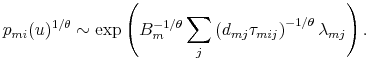
![\displaystyle P_{ei} =\left[ \int p_{ei}(v)^{1-\eta }\varphi _{e}(v)dv\right] ^{\frac{1}{ 1-\eta }}](img86.gif) and and ![\displaystyle P_{mi} =\left[ \int p_{mi}(u)^{1-\eta }\varphi _{m}(u)du\right] ^{\frac{1}{ 1-\eta }}](img87.gif) |
We explain how we derive the price indices for each country in appendix A. Given the assumption on the country-specific densities,
![\displaystyle P_{ei} =\gamma B_{e}\left[ {\sum\limits_{l}\left( d_{el}\tau _{eil}\right) ^{-1/\theta }\lambda _{el}}\right] ^{-\theta }](img90.gif) and and ![\displaystyle P_{mi} =\gamma B_{m}\left[ {\sum\limits_{l}\left( d_{ml}\tau _{mil}\right) ^{-1/\theta }\lambda _{ml}}\right] ^{-\theta },](img91.gif) |
where the unit costs for input bundles
The prices of the final good and structures are simply their marginal costs.
 and and |
For each tradable sector the fraction of country ![]() 's expenditure on imports from country
's expenditure on imports from country ![]() is given by
is given by
 and and  |
An alternative interpretation of
2.4 Equilibrium
We first define total factor usage in the intermediate goods sector in country ![]() as follows:
as follows:
 |
||
 |
||
 and and |
||
 |
where
The factor market clearing conditions in country ![]() are
are
The left-hand side of each of the previous equations is simply the factor usage by each sector, while the right-hand side is the factor availability.
The next three conditions require that the quantity of consumption and investment goods purchased by the household must equal the amounts available in country ![]() :
:
Aggregating over all producers of individual goods in each sector of country ![]() and using the fact that each producer minimizes costs, the factor demands at the sectoral level are described
by
and using the fact that each producer minimizes costs, the factor demands at the sectoral level are described
by
where
 |
||
 |
||
The total expenditure by country
To close the model we impose balanced trade country by country.
 |
The left-hand side denotes country
This completes the description of the steady-state equilibrium in our model. We next turn to calibration of the model.
3 Calibration
We calibrate our model using data for a set of 84 countries for the year 2005. This set includes both developed and developing countries and accounts for about 80 percent of the world GDP as computed from version 6.3 of the Penn World Tables (see Heston, Summers, and Aten, 2009).
Our classification for capital goods and structures are the categories "Machinery and equipment" and "Construction", respectively, in the International Comparisons Program (ICP). Prices of capital goods and structures are taken from the 2005 benchmark study of the Penn World Tables. To link prices of capital goods with trade and production in capital goods, we use four-digit ISIC revision 3 categories. Production data are from INDSTAT4, a database maintained by UNIDO. The corresponding trade data are available at the four-digit SITC revision 2 level. We follow the correspondence created by Affendy, Sim Yee, and Satoru (2010) to link SITC with ISIC categories. Intermediate goods correspond to the manufacturing categories other than capital goods, as listed by the ISIC revision 3. For details on specific countries, data sources, and how we construct our data; see Appendix B.
3.1 Common parameters
We begin by describing the parameter values that are common to all countries; see Table 1. The discount factor ![]() is set to 0.96, in line with
common values in the literature. Following Alvarez and Lucas(2007), we set
is set to 0.96, in line with
common values in the literature. Following Alvarez and Lucas(2007), we set ![]() equal to 2 (this parameter is not quantitatively important for the question addressed in this
paper).3
equal to 2 (this parameter is not quantitatively important for the question addressed in this
paper).3
From now on, the capital stock ![]() denotes the Cobb-Douglas composite of the stocks of producer durables and structures:
denotes the Cobb-Douglas composite of the stocks of producer durables and structures:
![]() . The share of capital in GDP,
. The share of capital in GDP, ![]() , is set at
1/3, as in Gollin(2002). Using capital stock data from the BEA, Greenwood, Hercowitz, and Krusell (1997) measure the rates of depreciation for both producer durables and structures. We set our values in accordance with their estimates:
, is set at
1/3, as in Gollin(2002). Using capital stock data from the BEA, Greenwood, Hercowitz, and Krusell (1997) measure the rates of depreciation for both producer durables and structures. We set our values in accordance with their estimates:
![]() and
and
![]() . We also set the share of producer durables in composite capital,
. We also set the share of producer durables in composite capital, ![]() , at 0.56 in accordance with Greenwood, Hercowitz, and Krusell (1997).
, at 0.56 in accordance with Greenwood, Hercowitz, and Krusell (1997).
The parameters
![]() , and
, and ![]() , respectively, control the shares of value
added in intermediate goods, capital goods, structures, and final goods production. To calibrate
, respectively, control the shares of value
added in intermediate goods, capital goods, structures, and final goods production. To calibrate ![]() and
and ![]() , we employ the data on value added and total output available in INDSTAT 4 2010 database. To compute
, we employ the data on value added and total output available in INDSTAT 4 2010 database. To compute ![]() we compute value added shares in gross
output for construction for a set of 32 OECD countries, and average across these countries. Data on value added and gross output for OECD countries are taken from input-output tables in the STAN database maintained by OECD for the period "mid 2000s", http://stats.oecd.org/Index.aspx. We set the
value
we compute value added shares in gross
output for construction for a set of 32 OECD countries, and average across these countries. Data on value added and gross output for OECD countries are taken from input-output tables in the STAN database maintained by OECD for the period "mid 2000s", http://stats.oecd.org/Index.aspx. We set the
value ![]() at 0.39. To calibrate
at 0.39. To calibrate ![]() we employ the same input-output
tables. The share of intermediates in final goods is
we employ the same input-output
tables. The share of intermediates in final goods is ![]() . Our estimate of
. Our estimate of ![]() is 0.9. Alvarez and Lucas (2007) compute a share of 0.82 by excluding agriculture and mining from the final goods sector. Since we include agriculture and mining in final goods we obtain a larger estimate.)
is 0.9. Alvarez and Lucas (2007) compute a share of 0.82 by excluding agriculture and mining from the final goods sector. Since we include agriculture and mining in final goods we obtain a larger estimate.)
The parameter ![]() controls the dispersion in efficiency levels. We use a simulated method of moments methodology as in Simonovska and Waugh (2011) and estimate this to be
0.23.
controls the dispersion in efficiency levels. We use a simulated method of moments methodology as in Simonovska and Waugh (2011) and estimate this to be
0.23.
| Parameter | Description | Value |
| 0.33 | ||
| 0.31 | ||
| 0.31 | ||
| 0.39 | ||
| 0.90 | ||
|
|
depreciation rate of producer durables | 0.12 |
|
|
depreciation rate of structures | 0.06 |
| variation in efficiency levels | 0.23 | |
| share of producer durables in composite capital | 0.56 | |
| discount factor | 0.96 | |
| elasticity of subs in aggregator | 2 |
3.2 Country-specific parameters
We take the labor force ![]() from Penn World Tables version 6.3 (PWT63, see Heston, Summers, and Aten, 2009 ). Using data on prices and bilateral trade shares, in both capital
goods and intermediate goods, we calibrate the bilateral trade barriers in each sector using a structural relationship implied by our model:
from Penn World Tables version 6.3 (PWT63, see Heston, Summers, and Aten, 2009 ). Using data on prices and bilateral trade shares, in both capital
goods and intermediate goods, we calibrate the bilateral trade barriers in each sector using a structural relationship implied by our model:
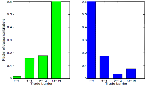
We set
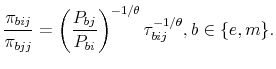
As can be seen in Figure 2 countries in the bottom decile of the income distribution face substantially larger barriers to export capital goods than countries in the top decile do. The figure displays the histogram of the cost for countries in each decile to export to all partners. The calibrated trade barriers in intermediate goods display a similar pattern: poor countries face larger barriers to export; we omit the figure for brevity.
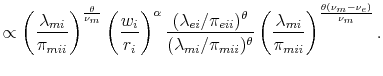
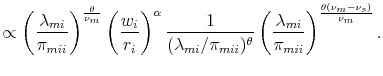
The remaining parameters include the productivity parameters
![]() and
and ![]() . Using data on relative prices, home trade
shares, and income per worker we use structural relationships to calibrate
. Using data on relative prices, home trade
shares, and income per worker we use structural relationships to calibrate


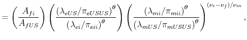
![\displaystyle = \left(\frac{A_{fi}}{A_{fUS}}\right) \left(\frac{\left(\lambda_{mUS}/\pi_{mUSUS}\right)^{\theta}}{\left(\lambda_{mi}/\pi_{mii}\right)^{\theta}}\right)^{\frac{1-\nu_{f}}{\nu_{m}}} \left[\left(\frac{\left(\lambda_{mUS}/\pi_{mUSUS}\right)^{\theta}}{\left(\lambda_{mi}/\pi_{mii}\right)^{\theta}}\right)^{\frac{1}{\nu_{m}}}\right]^{\frac{\alpha}{1-\alpha}}\times](img176.gif)
![\displaystyle \times \left[\left( \frac{\left(\lambda_{ei}/\pi_{eii}\right)^{\theta}}{\left(\lambda_{eUS}/\pi_{eUSUS}\right)^{\theta}} \frac{\left(\lambda_{mUS}/\pi_{mUSUS}\right)^{\theta}}{\left(\lambda_{mi}/\pi_{mii}\right)^{\theta}} \left(\frac{\left(\lambda_{mi}/\pi_{mii}\right)^{\theta}}{\left(\lambda_{mUS}/\pi_{mUSUS}\right)^{\theta}}\right)^{(\nu_{m}-\nu_{e})/\nu_{m}} \right)^{\mu} \right]^{\frac{\alpha}{1-\alpha}} \times](img177.gif)
![\displaystyle \times \left[\left( \frac{\left(\lambda_{mUS}/\pi_{mUSUS}\right)^{\theta}}{\left(\lambda_{mi}/\pi_{mii}\right)^{\theta}} \left(\frac{\left(\lambda_{mi}/\pi_{mii}\right)^{\theta}}{\left(\lambda_{mUS}/\pi_{mUSUS}\right)^{\theta}}\right)^{(\nu_{m}-\nu_{s})/\nu_{m}} \right)^{1-\mu} \right]^{\frac{\alpha}{1-\alpha}}](img178.gif)
We normalize
The average productivity gap in the capital goods sector between countries in the top and bottom deciles is 3.65. In the intermediate goods sector the average productivity gap is 1.90. This implies that rich countries have a comparative advantage in capital goods production, while poor countries have a comparative advantage in intermediate goods production.
4 Results
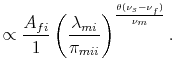
We define income per worker, at PPP, to be total factor income divided by the price of the final good:
![]() . Using arguments analogous to Waugh (2010), income per worker can be written as
. Using arguments analogous to Waugh (2010), income per worker can be written as
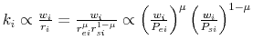
In the appendix we show that capital stock per worker is
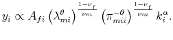
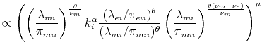
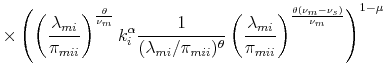
![% latex2html id marker 4479 $\displaystyle k_{i}\propto \left[ \left(\frac{\lambda_{mi}}{\pi_{mii}}\right)^{\frac{\theta}{\nu_{m}}} \left(\frac{(\lambda_{ei}/\pi_{eii})^{\theta}}{(\lambda_{mi}/\pi_{mii})^{\theta}}\left(\frac{\lambda_{mi}}{\pi_{mii}}\right)^{\frac{\theta(\nu_{e}-\nu_{m})}{\nu_{m}}}\right)^{\mu} \left(\frac{1}{(\lambda_{mi}/\pi_{mii})^{\theta}}\left(\frac{\lambda_{mi}}{\pi_{mii}}\right)^{\frac{\theta(\nu_{s}-\nu_{m})}{\nu_{m}}}\right)^{1-\mu} \right]^{\frac{1}{1-\alpha}}.$](img183.gif)
In equation (5)
![]() and
and ![]() are calibrated parameters. The remaining components on the
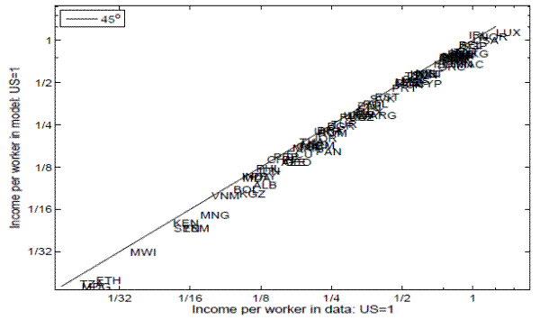
right-hand side of equation (5) are equilibrium objects. Figure 3 illustrates the relative income per worker in the model and in the data. Income per worker was one of the calibration targets and the model parameters
fit the target well. The final goods TFP,
are calibrated parameters. The remaining components on the
right-hand side of equation (5) are equilibrium objects. Figure 3 illustrates the relative income per worker in the model and in the data. Income per worker was one of the calibration targets and the model parameters
fit the target well. The final goods TFP, ![]() , does not affect the trade shares and , consequently, does not affect capital per worker. Hence,
, does not affect the trade shares and , consequently, does not affect capital per worker. Hence, ![]() simply scales income per worker in country
simply scales income per worker in country ![]() .
.
Much of the variation in income per worker is due to variation in ![]() . If we set
. If we set ![]() in each country to equal that in the U.S., capital per worker and home trade shares in equation (5) remain the same, but the log variance in income per worker declines from 1.05 to 0.29.
in each country to equal that in the U.S., capital per worker and home trade shares in equation (5) remain the same, but the log variance in income per worker declines from 1.05 to 0.29.
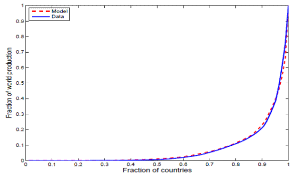
Figure 4 illustrates the cdf for capital goods production in the model along with its empirical counterpart. The model captures the observed skewness in production. Furthermore, the correlation between model and data for capital goods production is 0.94, so the countries are in fact lining up correctly in Figure 4.
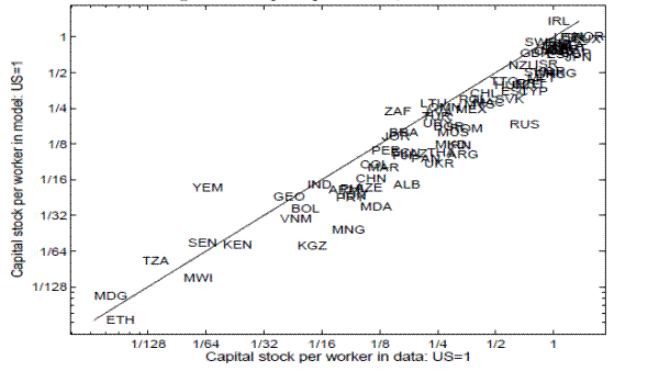
Equation (6) explicitly shows how trade affects capital per worker in each country. Trade in both intermediate goods, and in capital goods affects capital acumulation through the home trade shares ![]() and
and ![]() . Figure 5 plots capital per worker in the model against
capital per worker in the data. Although we did not target capital per worker directly, the model matches capital per worker for each country almost perfectly; the model explains 94 percent of the observed log variance in capital per worker.
. Figure 5 plots capital per worker in the model against
capital per worker in the data. Although we did not target capital per worker directly, the model matches capital per worker for each country almost perfectly; the model explains 94 percent of the observed log variance in capital per worker.
Next we present results along the trade dimension. In our calibration we targeted relative trade shares,
![]() , for each sector
, for each sector
![]() ; see equation (1). The levels of home trade shares,
; see equation (1). The levels of home trade shares, ![]() , are objects that we did not directly target. Figure 6 plots the levels of home trade shares in capital goods,
, are objects that we did not directly target. Figure 6 plots the levels of home trade shares in capital goods, ![]() , in the model against the data. The observations line up close to the 45 degree line and the correlation between model and data is 0.97. The home trade shares for intermediate goods also line up closely with the data. The correlation between model and data intermediate
goods home trade shares is 0.94.
, in the model against the data. The observations line up close to the 45 degree line and the correlation between model and data is 0.97. The home trade shares for intermediate goods also line up closely with the data. The correlation between model and data intermediate
goods home trade shares is 0.94.
In our model poor countries have a comparative advantage in intermediate goods while rich countries have a comparative advantage in capital goods. This result implies that model is consistent with the observation that poor countries are net importers of capital goods.
![Figure 6: Home trade share in capital goods.Figure 6 plots the levels of home trade shares in capital goods, pieii, in the model against the data. This single panel figure is a scatter plot with a 45 degree line. The line is a regression line that slopes upward to the right. Each data point represents a country in the sample. The y-axis is labeled,Home trades in intermediate goods in model and ranges from 0 to 0.8. The x-axis is labeled, Home trade share in intermediate goods in data and ranges from 0 to 0.8. The data points lie close to the regression line. Most of the data points are clustered at around [0.05, 0.1].](figure6.gif)
4.1 Misallocation due to trade barriers
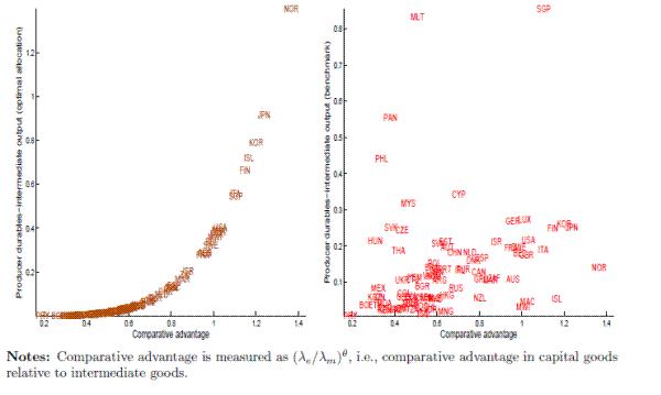
In the benchmark model trade barriers result in a misallocation of resources across sectors in each country. To highlight the magnitude of the misallocation, we compare the optimal allocation in a world without trade distortions with that in the benchmark model. In this exercise, we remove
barriers to trade in both sectors by setting
![]() for all countries and leaving all other parameters at their calibrated values. Clearly, the optimal allocation would dictate that countries with a comparative
advantage in capital goods should produce more capital goods relative to intermediate goods. Figure 7 plots the optimal relative size of the capital goods sector (
for all countries and leaving all other parameters at their calibrated values. Clearly, the optimal allocation would dictate that countries with a comparative
advantage in capital goods should produce more capital goods relative to intermediate goods. Figure 7 plots the optimal relative size of the capital goods sector (
![]() ) in each country in the left panel, and that for the benchmark model in the right panel. In a world with distortions, the relative size of the capital goods sector is far from
being optimal. The production of capital goods, relative to intermediate goods, is too little in rich countries and too much in poor countries. In the benchmark economy Panama allocates 87 times as much labor to capital goods production relative to the optimal allocation, and France allocates only
0.75 times as much.
) in each country in the left panel, and that for the benchmark model in the right panel. In a world with distortions, the relative size of the capital goods sector is far from
being optimal. The production of capital goods, relative to intermediate goods, is too little in rich countries and too much in poor countries. In the benchmark economy Panama allocates 87 times as much labor to capital goods production relative to the optimal allocation, and France allocates only
0.75 times as much.
Figure 7: Output in capital goods relative to intermediate goods: free trade (left), bench- mark (right)
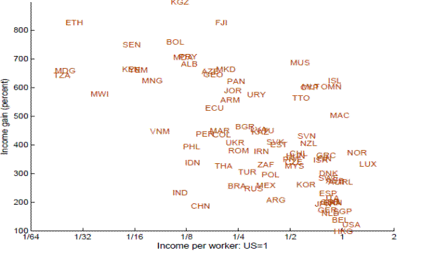
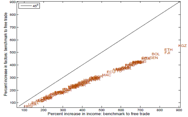
Poor countries gain substantially more than rich countries; see Figure 8. Countries in the bottom decile of the income distribution gain roughly twice as much as countries in the top decile. On average, increased capital accumulation accounts for 66 percent of the income gains; see Figure 9.
4.2 The role of trade in capital goods
Capital goods trade affects cross-country differences in income per worker in our model through two channels: 1) capital per worker, since capital stock in each country is not solely due to domestic capital formation (![]() in equation (6) affects
in equation (6) affects ![]() ), and 2) a component of TFP, since the trade balance condition connects capital
goods trade with intermediate goods trade and the home trade share in intermediate goods,
), and 2) a component of TFP, since the trade balance condition connects capital
goods trade with intermediate goods trade and the home trade share in intermediate goods, ![]() , affects the income per worker in equation (5). To
understand the role of capital goods trade, we eliminate all trade in capital goods by setting
, affects the income per worker in equation (5). To
understand the role of capital goods trade, we eliminate all trade in capital goods by setting
![]() to prohibitively high levels for all country pairs and leave all other parameters at their calibrated values. Countries trade only in intermediate goods in this experiment, so the
trade balance condition implies that exports of intermediate goods must equal the imports of intermediate goods in each country.
to prohibitively high levels for all country pairs and leave all other parameters at their calibrated values. Countries trade only in intermediate goods in this experiment, so the
trade balance condition implies that exports of intermediate goods must equal the imports of intermediate goods in each country.
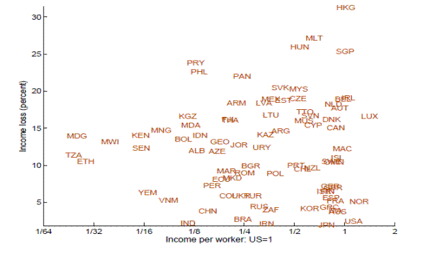
In the benchmark case many poor countries are net exporters of intermediate goods and net importers of capital goods. Once capital goods trade is shut down, they can no longer import capital goods. This distorts the world pattern of capital goods production toward countries that are inefficient at producing them, the poor countries. Thus, countries have to divert resources away from their sector of comparative advantage and poor countries lose 11 percent in income per worker. Figure 10 shows the income loss for every country as a result of eliminating trade in capital goods. In each country almost all of the decline in income per worker is due to decreased capital formation.
5.Conclusion
In this paper, we embed a multi-country multi-sector Ricardian model of trade into a neoclassical growth framework. By calibrating our model to bilateral trade shares, relative prices, and income per worker our model successfully reproduces the cross-country patterns in capital per worker, and capital goods production and home trade shares.
References
Affendy, Arip M., Lau Sim Yee, and Madono Satoru. 2010. "Commodity-industry Classification Proxy: A Correspondence Table Between SITC revision 2 and ISIC revision 3." MPRA Paper 27626, University Library of Munich, Germany. URL http://ideas.repec.org/p/pra/mprapa/27626.html.
Alvarez, Fernando and Robert E. Lucas. 2007. "General Equilibrium Analysis of the Eaton-Kortum Model of International Trade." Journal of Monetary Economics 54 (6):1726-1768.
Bernard, Andrew B., Jonathan Eaton, J. Bradford Jensen, and Samuel Kortum. 2003. "Plants and Productivity in International Trade." American Economic Review 93 (4):1268-1290.
Buera, Francisco J. and Yongseok Shin. 2010. "Financial Frictions and the Persistence of History: A Quantitative Exploration." NBER Working Papers 16400, National Bureau of Economic Research, Inc.
Caselli, Francesco. 2005. "Accounting for Cross-Country Income Differences." In Handbook of Economic Growth, edited by Philippe Aghion and Steven Durlauf, Handbook of Economic Growth, chap. 9. Elsevier, 679-741.
Dornbusch, Rudiger, Stanley Fischer, and Paul A. Samuelson. 1977. "Comparative Advantage, Trade, and Payments in a Ricardian Model with a Continuum of Goods." American Economic Review 67 (5):823-839.
Eaton, Jonathan and Samuel Kortum. 2001. "Trade in Capital Goods." European Economic Review 45:1195-1235.
Eaton, Jonathan and Samuel Kortum. 2002. "Technology, Geography, and Trade." Econometrica 70 (5):1741-1779.
Gollin, Douglas. 2002. "Getting Income Shares Right." Journal of Political Economy 110 (2):458-474.
Greenwood, Jeremy, Zvi Hercowitz, and Per Krusell. 1997. "Long-Run Implications of Investment-Specific Technological Change." American Economic Review 87 (3):342-362.
Greenwood, Jeremy, Juan M. Sanchez, and Cheng Wang. 2010. "Quantifying the Impact of Financial Development on Economic Development." Working Paper 10-05, Federal Reserve Bank of Richmond. URL http://ideas.repec.org/p/fip/fedrwp/10-05.html.
Guner, Nezih, Gustavo Ventura, and Xu Yi. 2008. "Macroeconomic Implications of Size-Dependent Policies." Review of Economic Dynamics 11 (4):721-744.
Hall, Robert E. and Charles I. Jones. 1999. "Why Do Some Countries Produce So Much More Output per Worker than Others?" Quarterly Journal of Economics 114 (1):83-116.
Heston, Alan, Robert Summers, and Bettina Aten. 2009. "Penn World Table Version 6.3." Center for International Comparisons of Production, Income and Prices at the University of Pennsylvania.
Klenow, Peter and Andres Rodriguez-Clare. 1997. "The Neoclassical Revival in Growth Economics: Has It Gone Too Far?" In NBER Macroeconomics Annual 1997, Volume 12, NBER Chapters. National Bureau of Economic Research, Inc, 73-114.
Restuccia, Diego and Richard Rogerson. 2008. "Policy Distortions and Aggregate Productivity with Heterogeneous Plants." Review of Economic Dynamics 11 (4):707-720.
Simonovska, Ina and Michael E Waugh. 2011. "The Elasticity of Trade: Estimates and Evidence." Tech. rep.
UNIDO. 2010. International Yearbook of Industrial Statistics 2010. Edward Elgar Publishing.
Waugh, Michael E. 2010. "International Trade and Income Differences." American Economic Review 100 (5):2093-2124.
A. Derivations
In this section we show how to derive analytical expressions for price indices and trade shares. The following derivations rely on three properties of the exponential distribution.
- 1)
-
 and
and
 .
. - 2)
-
 and
and
 .
. - 3)
-
and
 Pr
Pr .
.
A.1 Price indices
Here we derive the price index for intermediate goods, ![]() . The price index for capital goods can be derived in a similar manner. Cost minimization by producers of tradable good
. The price index for capital goods can be derived in a similar manner. Cost minimization by producers of tradable good
![]() implies a unit cost of an input bundle used in sector
implies a unit cost of an input bundle used in sector ![]() , which we denote by
, which we denote by
![]() .
.
Perfect competition implies that price in country ![]() of the individual intermediate good
of the individual intermediate good ![]() , when purchased from country
, when purchased from country ![]() , equals unit cost in country
, equals unit cost in country ![]() times the trade barrier
times the trade barrier
where
Since
Then, property 2 implies that
![\displaystyle \min_{j}\left[\left(d_{mj}\tau_{mij}\right)^{1/\theta}u_{j}\right]% \sim\exp\left(\sum_{j}\left(d_{mj}\tau_{mij}\right)^{-1/\theta}\lambda_{mj}\right).](img216.gif) |
Lastly, appealing to property 1 again,
Now let
 |
Apply a change of variables so that
 |
Let
![\displaystyle \gamma B_{m}\left[\sum_{j}(d_{mj}\tau_{mij})^{-1/\theta}\lambda_{mj}\right]% ^{-\theta}.](img226.gif)
A.2 Trade shares
We now derive the trade shares ![]() , the fraction of
, the fraction of ![]() 's total spending on
intermediate goods that was obtained from country
's total spending on
intermediate goods that was obtained from country ![]() . Due to the law of large numbers, the fraction of goods that
. Due to the law of large numbers, the fraction of goods that ![]() obtains from
obtains from ![]() is also the probability, that for any intermediate good
is also the probability, that for any intermediate good ![]() , country
, country ![]() is the least cost supplier. Mathematically,
is the least cost supplier. Mathematically,
where we have used equation (7) along with properties 2 and 3. Trade shares in the capital goods sector are derived identically.
A.3 Relative prices
Here we derive equations for three relative prices:
![]() , and
, and
![]() . Equations (8) and (9) imply that
. Equations (8) and (9) imply that
 |
||
 |
which implies that
 . Similarly,
 |
 |
 |
We show how to solve for
 |
||
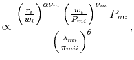
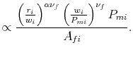
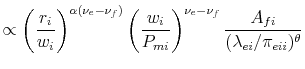
![\displaystyle =\frac{A_{fi}}{(\lambda_{ei}/\pi_{eii})^{\theta}} \left(\frac{r_{i}}{w_{i}}\right)^{\alpha(\nu_{e}-\nu_{f})} \left[\left(\frac{w_{i}}{r_{i}}\right)^{\alpha} \left(\frac{\lambda_{mi}}{\pi_{mii}}\right)^{\theta/\nu_{m}}\right]^{\nu_{e}-\nu_{f}}](img247.gif) |
||
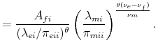 |
Similarly,
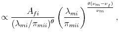 |
 |
A.4 Capital stock
We now derive an expression for the aggregate stock of capital per worker, ![]() . First note that
. First note that
![]() . Therefore,
. Therefore,
 .4 We show how to derive
![]() by making use of the relative prices derived above
by making use of the relative prices derived above
 |
||
|
(12) |
Analogously,
 |
Again, use the fact that
|
||
 |
||
![\displaystyle =\left[ \left(\frac{\lambda_{mi}}{\pi_{mii}}\right)^{\frac{\theta}{\nu_{m}}} \left(\frac{(\lambda_{ei}/\pi_{eii})^{\theta}}{(\lambda_{mi}/\pi_{mii})^{\theta}}\left(\frac{\lambda_{mi}}{\pi_{mii}}\right)^{\frac{\theta(\nu_{e}-\nu_{m})}{\nu_{m}}}\right)^{\mu} \left(\frac{1}{(\lambda_{mi}/\pi_{mii})^{\theta}}\left(\frac{\lambda_{mi}}{\pi_{mii}}\right)^{\frac{\theta(\nu_{s}-\nu_{m})}{\nu_{m}}}\right)^{1-\mu} \right]^{\frac{1}{1-\alpha}}.](img267.gif)
|
Categories
Capital goods in our model corresponds with " Machinery & equipment" in the ICP, (http://siteresources.worldbank.org/ICPEXT/Resources/ICP_2011.html). We identify the corresponding categories according to 4 digit ISIC revision 3 (for a complete list go to http://unstats.un.org/unsd/cr/registry/regcst.asp?cl=2). The ISIC categories for capital goods are: 2811, 2812, 2813, 2893, 2899, 291*, 292*, 30**, 31**, 321*, 322*, 323*, 331*, 332*, 3420, 351*, 352*, 353*, and 3599. Intermediate goods are identified as all of manufacturing categories 15**-37**, excluding those that are identified as capital goods. Structures in our model corresponds to ISIC categories 45** labeled " Construction". Final goods in our model correspond to the remaining ISIC categories excluding capital goods, intermediate goods, and structures.
Prices
Data on the prices of capital goods across countries are constructed by the ICP (available at http://siteresources.worldbank.org/ICPEXT/Resources/ICP_2011.html). We use the variable PX.WL, which is the PPP price of " Machinery & equipment", world price equals 1. The price of structures is also taken from the ICP; we use the variable PX.WL, which is the PPP price of " Construction", world price equals 1. The price of final goods in our model is taken to be the price consumption goods from PWT63 as the variable PC. The price of structures is (need to complete). The price of intermediate goods is (need to complete).
National accounts
PPP income per worker is taken from PWT63 as the variable RGDPWOK. The size of the workforce is constructed by taking other variables from PWT63 as follows: number of workers equals 1000*POP*RGDPL/RGDPWOK.
Production
Data on manufacturing production is taken from INDSTAT4, a database maintained by UNIDO (2010) at the four-digit ISIC revision 3 level. We aggregate the four-digit categories into either capital goods or intermediate goods using the classification method discussed above. Most countries are taken from the year 2005, but for this year some countries have no available data. For such countries we look at the years 2002, 2003, 2004, and 2006, and take data from the year closest to 2005 for which it is available, then convert into 2005 values by using growth rates of total manufacturing output over the same period.
Trade barriers
Trade costs are assumed to be a function of distance, common language, and shared border. All three of these gravity variables are taken from Centre D'Etudes Prospectives Et D'Informations Internationales (http://www.cepii.fr/welcome.htm).
Trade flows
Data on bilateral trade flows are obtained from UN Comtrade for the year 2005 (http://comtrade.un.org/). All trade flow data is at the four-digit SITC revision 2 level, and then aggregated into respective categories as either capital goods or intermediate goods. In order to link trade data to production data we employ the correspondence provided by Affendy, Sim Yee, and Satoru (2010) which links ISIC revision 3 to SITC revision 2 at the 4 digit level.
Construction of trade shares
The empirical counterpart to the model variable ![]() is constructed following Bernard, Eaton, Jensen and Kortum (2003) (recall that this is the fraction of country
is constructed following Bernard, Eaton, Jensen and Kortum (2003) (recall that this is the fraction of country
![]() 's spending on intermediates that was produced in country
's spending on intermediates that was produced in country ![]() ). We divide the value
of country
). We divide the value
of country ![]() 's imports of intermediates from country
's imports of intermediates from country ![]() , by
, by ![]() 's gross production of intermediates minus
's gross production of intermediates minus ![]() 's total exports of intermediates (for the whole
world) plus
's total exports of intermediates (for the whole
world) plus ![]() 's total imports of intermediates (for only the sample) to arrive at the bilateral trade share. Trade shares for the capital goods sector are obtained similarly.
's total imports of intermediates (for only the sample) to arrive at the bilateral trade share. Trade shares for the capital goods sector are obtained similarly.
C. Table
| Country | Isocode | Aθfi | λθei | λθmi | ((λei)/(λmi))θ |
| Albania | ALB | 0.29 | 0.24 | 0.43 | 0.56 |
| Argentina | ARG | 0.71 | 0.19 | 0.32 | 0.58 |
| Armenia | ARM | 0.58 | 0.13 | 0.33 | 0.39 |
| Australia | AUS | 0.90 | 0.85 | 0.92 | 0.93 |
| Austria | AUT | 0.91 | 0.49 | 0.79 | 0.62 |
| Azerbaijan | AZE | 0.42 | 0.16 | 0.51 | 0.32 |
| Belgium | BEL | 0.93 | 0.47 | 0.49 | 0.96 |
| Bolivia | BOL | 0.32 | 0.12 | 0.50 | 0.24 |
| Brazil | BRA | 0.47 | 0.39 | 0.71 | 0.54 |
| Bulgaria | BGR | 0.48 | 0.31 | 0.61 | 0.50 |
| Canada | CAN | 0.89 | 0.61 | 0.79 | 0.77 |
| Chile | CHL | 0.81 | 0.42 | 0.79 | 0.54 |
| China | CHN | 0.43 | 0.35 | 0.54 | 0.65 |
| Colombia | COL | 0.46 | 0.26 | 0.62 | 0.41 |
| Cyprus | CYP | 0.75 | 0.45 | 0.66 | 0.67 |
| Czech Republic | CZE | 0.70 | 0.31 | 0.75 | 0.40 |
| Denmark | DNK | 0.79 | 0.59 | 0.80 | 0.74 |
| Ecuador | ECU | 0.37 | 0.28 | 0.62 | 0.45 |
| Estonia | EST | 0.60 | 0.31 | 0.50 | 0.61 |
| Ethiopia | ETH | 0.17 | 0.08 | 0.30 | 0.28 |
| Fiji | FJI | 0.44 | 0.26 | 0.50 | 0.51 |
| Finland | FIN | 0.80 | 0.97 | 0.86 | 1.12 |
| France | FRA | 0.86 | 0.84 | 0.91 | 0.92 |
| Georgia | GEO | 0.46 | 0.17 | 0.41 | 0.41 |
| Germany | GER | 0.83 | 0.81 | 0.87 | 0.92 |
| Greece | GRC | 0.86 | 0.65 | 0.83 | 0.77 |
| Hong Kong | HKG | 1.07 | 0.17 | 0.28 | 0.61 |
| Hungary | HUN | 0.69 | 0.21 | 0.75 | 0.28 |
| Iceland | ISL | 0.88 | 0.87 | 0.76 | 1.14 |
| India | IND | 0.33 | 0.31 | 0.55 | 0.56 |
| Indonesia | IDN | 0.40 | 0.16 | 0.51 | 0.30 |
| Iran | IRN | 0.67 | 0.38 | 0.66 | 0.58 |
| Ireland | IRL | 0.97 | 0.59 | 0.86 | 0.69 |
| Israel | ISR | 0.83 | 0.65 | 0.76 | 0.85 |
| Italy | ITA | 0.89 | 0.98 | 0.91 | 1.08 |
| Japan | JPN | 0.85 | 1.06 | 0.88 | 1.21 |
| Jordan | JOR | 0.43 | 0.32 | 0.59 | 0.54 |
| Kazakhstan | KAZ | 0.69 | 0.21 | 0.55 | 0.38 |
| Kenya | KEN | 0.25 | 0.13 | 0.40 | 0.32 |
| Korea, Republic of | KOR | 0.76 | 0.93 | 0.80 | 1.17 |
| Kyrgyzstan | KGZ | 0.41 | 0.10 | 0.36 | 0.27 |
| Latvia | LVA | 0.52 | 0.24 | 0.54 | 0.45 |
| Lithuania | LTU | 0.55 | 0.29 | 0.63 | 0.46 |
| Luxembourg | LUX | 1.15 | 0.54 | 0.55 | 0.98 |
| Macao | MAC | 1.13 | 0.42 | 0.42 | 0.99 |
| Macedonia | MKD | 0.41 | 0.31 | 0.55 | 0.56 |
| Madagascar | MDG | 0.13 | 0.10 | 0.21 | 0.49 |
| Malawi | MWI | 0.21 | 0.17 | 0.17 | 0.97 |
| Malaysia | MYS | 0.85 | 0.30 | 0.69 | 0.43 |
| Malta | MLT | 0.79 | 0.30 | 0.63 | 0.48 |
| Mauritius | MUS | 1.07 | 0.25 | 0.57 | 0.44 |
| Mexico | MEX | 0.53 | 0.22 | 0.75 | 0.29 |
| Moldova | MDA | 0.39 | 0.12 | 0.38 | 0.32 |
| Mongolia | MNG | 0.26 | 0.14 | 0.24 | 0.61 |
| Morocco | MAR | 0.48 | 0.40 | 0.49 | 0.82 |
| Netherlands | NLD | 0.83 | 0.43 | 0.59 | 0.72 |
| New Zealand | NZL | 0.74 | 0.64 | 0.83 | 0.77 |
| Norway | NOR | 1.06 | 1.15 | 0.86 | 1.33 |
| Oman | OMN | 1.16 | 0.37 | 0.75 | 0.50 |
| Panama | PAN | 0.41 | 0.18 | 0.50 | 0.35 |
| Paraguay | PRY | 0.36 | 0.08 | 0.48 | 0.16 |
| Peru | PER | 0.35 | 0.29 | 0.64 | 0.45 |
| Philippines | PHL | 0.40 | 0.15 | 0.49 | 0.31 |
| Poland | POL | 0.56 | 0.42 | 0.75 | 0.56 |
| Portugal | PRT | 0.64 | 0.47 | 0.78 | 0.61 |
| Romania | ROM | 0.44 | 0.35 | 0.63 | 0.55 |
| Russia | RUS | 0.55 | 0.45 | 0.68 | 0.66 |
| Senegal | SEN | 0.23 | 0.18 | 0.35 | 0.52 |
| Singapore | SGP | 1.04 | 0.43 | 0.40 | 1.07 |
| Slovak Republic | SVK | 0.61 | 0.24 | 0.68 | 0.35 |
| Slovenia | SVN | 0.74 | 0.41 | 0.72 | 0.57 |
| South Africa | ZAF | 0.61 | 0.59 | 0.70 | 0.84 |
| Spain | ESP | 0.84 | 0.72 | 0.92 | 0.78 |
| Sweden | SWE | 0.81 | 0.80 | 0.84 | 0.95 |
| Tanzania | TZA | 0.11 | 0.15 | 0.34 | 0.45 |
| Thailand | THA | 0.46 | 0.22 | 0.58 | 0.39 |
| Trinidad and Tobago | TTO | 0.80 | 0.39 | 0.77 | 0.50 |
| Turkey | TUR | 0.47 | 0.48 | 0.69 | 0.69 |
| Ukraine | UKR | 0.58 | 0.24 | 0.60 | 0.40 |
| United Kingdom | GBR | 0.84 | 0.85 | 0.86 | 0.99 |
| United States | USA | 1.00 | 1.00 | 1.00 | 1.00 |
| Uruguay | URY | 0.56 | 0.28 | 0.68 | 0.41 |
| Vietnam | VNM | 0.32 | 0.23 | 0.43 | 0.53 |
| Yemen | YEM | 0.15 | 0.25 | 0.54 | 0.46 |