Skip to: [Printable Version (PDF)] [Bibliography] [Footnotes]

System Committee on International Economic Analysis: Screen Reader version ^♣

Are Long-Term Inflation Expectations Well-Anchored in Brazil, Chile and Mexico?*

Michiel De Pooter	Patrice Robitaille*	Ian Walker	Michael Zdinak
Federal Reserve	Federal Reserve	Federal Reserve	Federal Reserve
Board	Board	Board	Board

March 2013
PRELIMINARY DRAFT. PLEASE DO NOT QUOTE

Abstract:

We examine whether long-term inflation expectations are well-anchored in Brazil, Chile, and Mexico, three emerging market countries with an explicit inflation targeting regime. We use survey measures on long-term inflation expectations as well as high-frequency far-forward inflation compensation measures based on financial market data. Because the latter have been unavailable to date for these countries, we constructed a sufficiently long historical daily time-series of these measures from sovereign bond prices. We first compare the survey and market-based long-run inflation expectations and find that these do not necessarily imply the same conclusion; whereas survey measures typically track each country's inflation target quite well, the high-frequency measures are more volatile and regularly deviate from the inflation target. We then use our daily inflation compensation measures in an event study, regressing daily changes in inflation compensation on news surprises of monetary policy, prices, and the real economy. The results show that far-forward inflation compensation does not significantly react to domestic news surprises, implying that inflation expectations in Brazil, Chile, and Mexico are well-anchored. However, inflation compensation does react to some U.S. and Chinese news surprises. Subsample analysis shows that inflation expectations have become better anchored predominantly in recent years. Overall, we argue that it may be too premature to conclude that long-term inflations expectations in Brazil, Chile and Mexico have truly become well-anchored.
Keywords: Inflation targeting, survey expectations, inflation compensation, Nelson-Siegel
model, macro news suprises, Brazil, Chile, Mexico
JEL classification: D84, E31, E43, E44, E52, E58, G14

1 Introduction

Nearly 30 countries have adopted inflation targeting frameworks, driven by a conviction that defining an explicit inflation target and communicating how the central bank will strive to meet that goal is the best monetary policy strategy for maintaining inflation at a relatively low and stable level without sacrificing long-term growth.¹ Several studies have found that countries with inflation targeting frameworks have had lower inflation and generally better economic performance than countries without inflation targeting frameworks but it has not been clear whether it was adopting inflation targeting framework or other factors have been driving those results.² There is some evidence that an explicit inflation target can help coordinate private agents' inflation expectations and anchor long-term inflation expectations to the specified target (references below). However, due to data limitations, most of the work has focused on the experience of industrialized countries. In this study, we overcome some of these data limitations and we explore whether and to what degree long-term inflation expectations are well-anchored in three emerging market economies: Brazil, Chile, and Mexico.

The behavior of long-term inflation expectations provides insight into the success of inflation targeting as a monetary policy strategy. Unforeseen shocks can drive inflation away from the target, monetary policy influences inflation with a considerable lag, and there is uncertainty about the transmission process itself (Svensson, 1999 and many others make this point). These circumstances will influence inflation expectations over the short- and medium- term. Nonetheless, if the central bank is viewed as being committed to bringing inflation back to the inflation goal, shocks that affect inflation should be viewed as transitory and therefore should not influence long-term inflation expectations.

Because Brazil, Chile, and Mexico all have inflation targeting frameworks, this study can be thought of as an effort to look for within-group differences among inflation targeters, an area that has received relatively little attention. These three countries are at similar stages of development, have had inflation targeting frameworks in place for over a decade, and previously had a historical record of monetary and fiscal mismanagement. On the other hand, their inflation targeting frameworks have differed in several respects and have undergone changes over time³, and we would only be able to speculate on the reasons for differences that we find in the data.

Our approach is a blend of an informal and formal analysis. In our formal analysis, we follow the approach that was first used by Gurkaynak, Sack, and Wright (2007b) by examining both the evidence from surveys of inflation expectations as well as from financial market-derived measures of long-term inflation expectations. To the best of our knowledge, long-horizon financial market based expectations of future inflation with a sufficiently long history have been unavailable to date for Brazil, Chile and Mexico as a result of insufficient data on sovereign bond prices. We therefore first collected a comprehensive set of historical prices on nominal and inflation-linked sovereign bonds, and used these to construct far-forward inflation compensation estimates for each individual country. We use the Nelson, C. R. and A. F. Siegel (1987) model to estimate nominal and real zero coupon curves from all observed bond prices. We then measure inflation compensation at any desired (forward) horizon as the spread between these two curves. Inflation compensation provides a reading on investors' expectations for inflation plus the premium that investors demand for the risk that inflation may exceed its expected level.⁴ Far-forward inflation compensation covers a period that is several years in the future, beyond the period over which shocks to inflation and monetary policy influence the inflation outlook.

Because market-based measures of far-forward inflation expectations were previously unavailable for emerging market countries, studies that examined the success of inflation targeting in these countries were restricted to using only survey measures.⁵ We therefore also use to the extent possible surveys of long-term inflation expectations and the dispersion in these measures. Regarding the latter, Beechey, M. J., B. K. Johanssen, and A. T. Levin (2011) compare survey-based measures of long-term inflation expectations in the euro area with those for the United States and find that the dispersion of long-term inflation expectations was higher in the United States than in the euro area.⁶ The dispersion in inflation expectations - the degree of disagreement among forecasters - is considered to be a reasonable proxy for inflation uncertainty (the aggregate distribution of inflation forecasts). Using survey results from Consensus Economics, Capistran, C. and M. Ramos-Francia (2010) find that the dispersion in short- and medium-term inflation expectations is lower in countries with inflation targeting than in countries without. For our three countries, we use the survey data from Consensus Economics. Survey measures in general, however, are typically only available at relatively low frequencies; either monthly, quarterly, or even only semi-annually. In particular, readings on long-term inflation expectations for most inflation targeting countries are currently still only available at a semi-annual frequency. Consensus Economics provides survey expectations of inflation between five and ten years ahead only twice a year; in the fall and in spring, but does not provide a dispersion in respondents' expectations associated with the survey results.⁷ For Brazil and Mexico we are able to supplement the Consensus data with data from surveys of professional forecasters that are compiled by the central bank. With both the survey and market-based measures of inflation expectations in hand, we can compare the two measures to assess whether they convey differences in the degree to which countries' inflation targeting regimes are successful in shaping agents' expectations about future inflation.

Similar as in Gurkaynak, Levin, Marder, and Swanson (2007a) and Gurkaynak, Levin, and Swanson (2010a), among others, we can also assess whether our market-based measures of far-forward inflation compensation respond significantly to news surprises in monetary policy decisions, prices, and macroeconomic data releases. Gurkaynak et al. (2010a) find that long-term inflation expectations were better-anchored in Sweden, an inflation targeting country, than in the United States, which at that time did not have an explicit inflation target. Far-forward inflation compensation for Sweden did not significantly react to news suprises during a period from 1996 to 2005, while U.S. forward inflation compensation does significantly react to surprises during a very similar period (1998 to 2005). They also find that long-term inflation expectations in the United Kingdom became well anchored after the Bank of England gained legal independence in the late 1990s.⁸ Gurkaynak el al. (2007a) compare the experience of the United States with those of Canada and Chile, using data for the somewhat different periods for each country. Long-term inflation expectations were found to be well anchored in Canada and Chile, although the evidence for Chile is based on only a short sample period (2002 to 2004). Details on this empirical approach are Section 4 below. Galati,Poelhekke, and Zhou (2011) explore whether the global financial crisis unhinged long-term inflation expectations. Although the evidence is inconclusive, long-term inflation expectations in the United Kingdom drifted up.

What all these studies have in common, is that they have all focused on the experience of industrialized countries because market-based measures of long-term inflation expectations have been unavailable to date for many emerging market economies. The fact that long-term bond markets in Brazil, Chile, and Mexico have been developing allows us to construct our financial market-based inflation compensation measures. Although market liquidity for some long-term bonds in these country will certainly be an issue, we believe that it is well worth taking a closer look at what the results from the event study analysis imply.

After reviewing the evidence from our formal regressions, we conclude that although long-term inflation expectations seem to have become better anchored in all three countries over the past decade, it is premature to conclude that long-term inflation expectations are truly well-anchored. On the one hand, we did not find evidence that market participants systematically revised their views on long-term inflation in response to domestic macroeconomic and monetary policy news. This result, by itself, would suggest that long-term inflation expectations are well anchored. On the other hand, we find that inflation compensation does tend to react to certain foreign macroeconomic news suprises. Furthermore, the level of far-forward inflation compensation is persistently above the target in Brazil, and survey data provide some evidence that long-term inflation expectations may be drifting up. Far-forward inflation compensation has hovered above the inflation target in Mexico, particularly since 2009. And we do not have an explanation for the sizeable variations in far-forward inflation compensation for Chile.

A possible explanation for these results is that other types a news (with one candidate being the U.S. and Chinese surprises that we find to be significant) have been much more important drivers of long-term inflation expectations and the risk premium in these countries.

2 Inflation targeting in Brazil, Chile, and Mexico

2.1 Inflation Targeting in Brazil, Chile and Mexico

The top panels of Figures 1 through 3 display 12-month inflation (headline and core) in Brazil, Chile, and Mexico, as well as the inflation target and the tolerance range for the inflation targets. Brazil and Chile adopted inflation targeting frameworks in 1999 and Mexico adopted its inflation targeting framework in 2001.⁹ In 2001, while in the midst of disinflation, the Bank of Mexico announced that the inflation target would be 3 percent from 2003 on. Chile's inflation target was formally 2 to 4 percent range until January 2007, when a 3 percent inflation target was announced.¹⁰ Brazil's inflation target is set yearly and is announced a year and a half in advance. The target was reduced to a low of 3¼ percent for 2003 but was subsequently raised and has been 4½ percent since 2005.¹¹ Chile and Mexico have a tolerance range of 1 percentage point in each direction around the target while Brazil's is wider (2 percentage points since 2006).

3 Survey and market-based measures of inflation expectations

3.1 Survey-Based Inflation Expectations

The middle panels of Figures 2 to 4 display the inflation target against a widely used measure of long-term expected inflation from the Consensus Forecasts survey, which is taken in the spring and fall of every year. Consensus Forecasts releases the average of participants' expectations. Levin, Natalucci, and Piger (2004) showed that long-term inflation expectations had already been falling in the years preceding the adoption of formal inflation targets. Average expected inflation for Chile had been very close to 3 percent even before the formal 3 percent target was adopted in early 2007. Long-term inflation expectations for Mexico have been at or very near 3½ percent since 2005, ½ percentage point above the target. The Bank of Mexico's monthly survey of expectations first polled views on long-term inflation in 2008, and the average expectation from this survey has also been at about 3½ percent (blue line).

For Brazil, long-term inflation expectations have been more variable, jumping up during the 2002 crisis, then drifting down to below the (revised upward) inflation target, and then drifting up again to 4½ percent. One possible interpretation of these movements is that signals from government officials on the desirable level of long-term inflation have been unclear, and as a result, long-term expected inflation may be less well anchored than what otherwise would have been the case.¹² That is even if, for inflation targeting countries as a whole,Alichiet al.(2011) found that long-term inflation expectations in inflation targeting emerging market economies are less sensitive to changes in short-term inflation expectations than are countries with alternative monetary arrangements.¹³

3.2 Financial Market-Based Inflation Expectations

The drawback of using survey-based measures or realized inflation measures to assess how well-anchored are inflation expectations, which is what the emerging market literature so far has typically done, is that these measures are typically available only at relatively low frequencies; either monthly, quarterly, or even semi-annually. Long-horizon survey measures, which tend to be uncontaminated by short-term shocks to inflation and can therefore shed the most light on the behavior of inflation expectations, are currently only available at a semi-annual frequency.¹⁴. It is therefore difficult to truly gauge whether a central bank's inflation targeting regime is successful in shaping agents' expectations about future inflation.

Luckily, we can derive much higher-frequency gauges of inflation expectations from financial market data. Using data on inflation swaps and/or nominal and real interest rates, all typically available at a daily frequency, one can construct daily measures of (far-forward) inflation compensation.¹⁵ Market participants and policy makers alike heavily track these financial market-based measures to gauge the effect of macroeconomic news announcements or monetary policy decisions on market participants' perception of future inflation. Several studies, including Gurkaynak, Levin, Marder, and Swanson (2007a), Guurkaynak, Levin, and Swanson (2010a), Beechey, Johanssen, and Levin (2011), and Galati, Poelhekke, and Zhou (2011), have used these market-based inflation compensation measures in event study regression analyses to assess their sensitivity to macroeconomic news and to see how well-anchored inflation expectations are.

One important caveat to using these measures, however, is that they do necessarily offer a fully clean read on inflation expectations. As pointed out by Hordahl (2009), besides reflecting the level of expected inflation, inflation compensation also embed inflation risk premia, liquidity premia, and technical factors. It is difficult, if not impossible to distinguish these different factors without having to resort to strong identifying assumptions.

In this section we first construct inflation compensation measures for Brazil, Chile and Mexico. In particular, we use term structure estimation techniques to construct full term structures of inflation compensation at various horizons. To the best of our knowledge, we are the first to construct these measures in detail for Brazil, Chile and Mexico. We first construct a sufficiently large history of marked-based inflation compensation measures and then use these in Section 4 in an event study, similar to the studies mentioned above, to assess the sensitivity of inflation compensation to news surprises about monetary policy actions, prices, and the real economy.

3.2.1 Estimating inflation compensation measures

We estimate our financial market-based inflation compensation measures as the spread between yields on nominal and inflation-indexed (real) sovereign bonds. The latter bonds have a principal value that is linked to inflation and therefore protect investors from inflation risk. Brazil, Chile and Mexico all have had a history of monetary mismanagement resulting in periods of very high inflation. It should therefore not be surprising that each of these countries have substantial experience with issuing inflation-linked bonds.¹⁶ The fact that each country has a spectrum of both nominal and real sovereign bonds outstanding allows us to construct nominal and real zero-coupon curves from these bonds, respectively. The zero curve estimation method we apply is that of Nelson and Siegel (1987) which has increasingly become the workhorse method for estimating zero curves from bond prices.¹⁷

A zero-coupon yield curve consists of the collection of interest rates earned on non-coupon-paying bonds with increasing maturities. Because zero-coupon yields are not directly observable but are instead embedded in coupon-bearing bonds, we must resort to curve estimation techniques such as the Nelson and Siegel (1987) model. This model postulates that the curve of continuously-compounded zero -coupon yields at any given time can be well described by a smooth parametric function which is governed by just four parameters;

$\displaystyle y_{t}(\tau)=\beta_{1,t}+\beta_{2,t}\!\left[\frac{1-\exp\!{\left(\!-\frac{\tau}{\lambda_{t}}\right)}}{\left(\frac{\tau}{\lambda_{t}}\right)}\right]+\beta_{3,t}\!\left[\frac{1-\exp\!{\left(\!-\frac{\tau}{\lambda_{t}}\right)}}{\left(\frac{\tau}{\lambda_{t}}\right)}-\exp\!{\left(\!-\frac{\tau}{\lambda_{t}}\right)}\right]$

(1)

where $y_{t}(\tau)$ is the model-implied $\tau$ -period zero-coupon yield and $\{\beta_{1,t},\beta_{2,t}\beta_{3,t},\lambda_{t}\}$ is the parameter vector. These parameters can be interpreted as the level parameter, $\beta_{1,t}$ , the slope parameter, $\beta_{2,t}$ , and the curvature parameter, $\beta_{3,t}$ , judging from the effect that a change in each of these respective parameters has on the shape of the curve, see for example Diebold and Li (2006). The fourth parameter, $\lambda_{t}$ , is a shape parameter that influences the factor loading associated with the slope and curvature parameters. We follow the approach of Gurkaynak, Sack, and Wright (2007b) and Gurkaynak, Sack, and Wright (2010b) to estimate nominal and real zero coupon curves from observed bond prices. In particular, we estimate the Nelson-Siegel parameters by minimizing the sum of squared approximate yield errors; bond price fitting errors weighted by the inverse of modified duration ( MDur ):

$\displaystyle \min_{\{\beta_{1,t},\beta_{2,t}\beta_{3,t},\lambda_{t}\}} \sum_{i=1}^{N_{t}} \left[\frac{P_{i,t}(\tau)-\widehat{P_{i,t}}(\tau)}{\text{MDur}_{i,t}}\right]^{2}$

(2)

where $P_{i,t}(\tau)$ are the prices for $N_{t}$ observable bonds on day

, and $\widehat{P_{i,t}}(\tau)$ are the bond price estimates implied by the Nelson-Siegel model.

When implementing the Nelson-Siegel model we must ensure that the optimization procedure converges to sensible and reliable zero curves. To accomplish this we impose several restrictions on the model parameters: (i) the level parameter $\beta_{1,t}$ is restricted to be positive and in the range , (ii) the slope and curvature parameters, $\beta_{2,t}$ and $\beta_{3,t}$ , respectively, are restricted to be in the range , (iii) the shape parameter, $\lambda_{t}$ , is restricted to be contained in the range . As discussed below, we only include bonds in the optimization which have a remaining maturity between three months and 15 years. An immediate problem arising from this particular maturity window is that our estimated yield curves could show odd behavior for maturities between zero and three months. Specifically because there are no data points on short-term rates by construction, the short end of the curve could therefore in theory go to either plus of minus infinity. To prevent this, we impose that the Nelson-Siegel implied instantaneous short rate, the sum of $\beta_{1,t}$ and $\beta_{,2t}$ , has to be equal to the overnight rate, or, if the overnight rate shows erratic behaviour, the central banks' official target rate.¹⁸

Once we have estimates of the nominal and real zero coupon curves for each day in the sample for our three countries, we difference the two curves to construct an estimate of the inflation compensation curve. Furthermore, with the estimated Nelson-Siegel, we can construct zero yields for any desired maturity. We can also easily compute nominal and real forward rates, and therefore forward inflation compensation estimates. In the remainder of the paper we will focus primarily on 1-year far-forward rates: 1-year forward rates ending in 1, 2, ... , 7 years in the future for Brazil and Mexico and 1-year forward rates ending in 1, 2, ... , 10 years for Chile.

3.2.2 Bond Data

Brazil and Mexico
We collected historical prices on nominal and inflation-linked bonds for Brazil and Mexico from several sources. Because our goal iss to construct long-enough time series of far-forward inflation compensation, we combined data from different sources. For Brazil we obtained daily prices for all current and previously outstanding bonds from Bloomberg and MorganMarkets.¹⁹ For Mexico we combined data from Bloomberg and Proveedor Integral de Precios (PIP).²⁰

As is standard practice, we apply the usual filters to the available bond data; we do not include any bonds that have option-like features or floating coupon payments, and we do not include any Treasury bills out of concern that the behavior of bills can be quite different from that of bonds. From the remaining bonds, on any given day we only include those bonds that have a remaining maturity between three months and fifteen years.²¹ The top two panels of Figure 4 show the number of bonds over time that were included in the estimation.²² For both Brazil and Mexico, the number of outstanding bonds has increased throughout the sample, in particular for nominal bonds. The total number of bonds continues to remains relatively small, however, likely introducing some degree of noise in our curve estimates. To shed some light on this issue, Figure 5 shows the average absolute bond price fitting error for bonds with maturities between two and ten years. This metric is used in for example Gurkaynak, Sack, and Wright (2010b) to assess the fit of zero coupon curve models. On average, we fit bond prices with an error of about 0.25%. This is higher than the yield fitting errors that Gurkaynak, Sack, and Wright (2010b) report for likely more-liquid U.S. Treasury Inflation Protected Securities, but is certainly reasonable.²³ Note that for both Brazil and Mexico the fitting errors, in particular for inflation-index bonds in Mexico, spiked up in the 4 $^{th}$ quarter of 2008 when both countries underwent a sudden stop with investors partially withdrawing from the countries.²⁴

The bottom panels of Figure 4 show the longest-maturity bond used in the estimation. Panel C shows that Brazil did not issue its first long-maturity nominal bond until July 2006. We therefore start our data sample for Brazil in July 2006. Furthermore, even though Brazil has issued 10-year bonds at several times throughout our sample, the longest maturity that is consistently outstanding throughout the sample is seven years. In order to prevent having to extrapolate our zero-coupon curves for longer maturities, we therefore estimate our curves only up to maturities of seven years. We do the same for Mexico.²⁵

Chile

For Chile we use nominal and real zero coupon curves that were graciously supplied to us by RiskAmerica.²⁶. RiskAmerica estimates zero-coupon curves from prices on Chilean nominal and inflation-linked sovereign bonds, in a comparable fashion as we do here for Brazil and Mexico. RiskAmerica's zero coupon estimates were similarly used by Gurkaynak et al. (2007a) to construct 1-year forward inflation compensation rates when they examined whether inflation expectations were well-anchored in Chile between August 2002 and October 2005 (see the discussion in Section 4. Compared to Gurkaynak et al. (2007a) our sample for Chile is much longer; October 2, 2002 to October 18, 2012.

As noted by Gurkaynak et al. (2007a), it was not until 2002 that Chile began issuing long-term nominal bonds.²⁷ However, since that time, the maturity of the longest-outstanding bond has consistently been above ten years. We therefore use 1-year forward inflation compensation rates ending in 10 years, similar to Gurkaynak et al. (2007a), and in contrast to our forward inflation compensation measures for Brazil and Mexico, which end in seven years. Because Chilean forward rates are also based on fewer bonds in comparison to for example U.S. and U.K. forward rates, they will tend to be more noisy.²⁸

3.2.3 Far-forward inflation compensation estimates

Figure 6 shows our market-based time-series estimates of far-forward nominal yields in Panel A, far-forward real yields in Panel B, and far-forward inflation compensation in Panel C. The far-forward inflation compensation measures in the bottom panel are the spread between the forward rates in the top two panels. Far forward inflation compensation is also plotted in the bottom panels of Figures 1 to 3. We make 3 observations here. First, the fact that all three governments were able to issue long-term nominal debt by the mid-2000s is a sign that inflation expectations have become better anchored, for previously, investors had demanded higher yields for long-term debt than what governments were willing to pay. Second, far forward inflation compensation varies considerably, particularly for Brazil, where it spikes in late 2008. Third, far forward inflation compensation for Brazil and Mexico has nearly always been above the inflation target but for Chile has been both below and above 3 percent.

Far forward inflation compensation for Mexico declines considerably between 2003 and 2005, and for a period in 2007 and 2008 is very close to 3½ percent. It appears that although financial market participants viewed the inflation target as higher than 3 percent, the inflation risk premium was seen as small. (In a future draft, we will obtain measures of the inflation risk premium by subtracting the Consensus measure of long-term expected inflation from inflation compensation.) The inflation compensation jumps up in 2009 and slowly moves down until late 2012.

4 Sensitivity of Yields and Inflation Compensation to News

Previous studies that use financial market-based estimates of far-forward inflation compensation to examine whether inflation expectations are well-anchored, e.g. Gurkaynak et al. (2005), Gurkaynak et al. (2007a), Gurkaynak et al. (2010a), and Beechey et al. (2011), have all focused on developed economies such as the U.S., U.K., Canada or Sweden. For emerging market economies, the lack of sufficiently-long time series of far-forward inflation compensation measures has, to date, precluded similar studies. Using the inflation compensation measures that we constructed in Section 3.2 we fill in this gap in the literature for Brazil, Chile and Mexico.²⁹

We build upon the regression analysis used in the studies referenced above by regressing daily changes in forward nominal and real yields and, in particular, far-forward inflation compensation on the surprise component of news announcements on monetary policy, prices, and the real economy, while controlling for several other factors that may influence inflation compensation. The premise here is that if inflation expectations are well-anchored, far-ahead forward inflation compensation should not react significantly to news surprises. If they do react significantly then this is a indication that agents' inflation expectations remain unhinged.

4.1 Regression Approach

We estimate the parameters of the following linear regression specification:

$\displaystyle \Delta y_{t,n} = \alpha_{n} + \beta_{n} X_{t} + \gamma_{n} Z_{t} + \epsilon_{t,n} \qquad \epsilon_{t,n} \sim IID(0.\sigma_{n}^{2})$

(3)

where $\Delta y_{t,n}$ is the daily change in either (forward) nominal and real rates or far-forward inflation compensation ending in

years³⁰ and $X_{t}$ is the vector of news surprises. We follow Galati, Poelhekke, and Zhou (2011) by also including a vector of control variables, $Z_{t}$ to control for the fact that inflation compensation not only reflects inflation expectations, but also inflation risk premia, liquidity, and technical factors. By including variables that are aimed at controlling for the latter two factors, we attempt to restrain the influence of variation in the liquidity and other technical factors not directly related to inflation expectations³¹.

We not only examine whether domestic news surprises move inflation compensation for Brazil, Chile, and Mexico, but also whether news surprises from the U.S. and China have a significant impact. All three countries that we analyze are open economies that rely heavily on imports and exports with the U.S. and China being major trading partners. It is therefore interesting to see whether developments abroad have an influence on inflation expectations at home.

In the end we are interested in which, if any, of the surprises included in the regression have a significant impact on inflation compensation. To assess whether, overall, inflation expectations are well-anchored or not, we perform a standard test of the joint hypothesis that all coefficients in the regression are equal to zero (i.e. $\beta_{n} = \gamma_{n} = 0$ ). Furthermore, Galati et al. (2011) examine the effect that the financial crisis that erupted in mid-2007 has had on the anchoring properties of inflation expectations in the U.S., U.K. and the euro area and find that expectations may have become less well-anchored. We therefore also examine subsamples of before and after mid-2007 to assess the stability of our full sample results.

4.2 News surprise data and controls

Similar to the previous literature, we include surprises on three types of announcements for which we have sufficient data available; news on (i) the stance of monetary policy, (ii) prices, (iii) the real economy. We included data on the following eight announcements (when available) in the regressions: (1) the central bank policy rate,³²(2) headline consumer prices (CPI), (3) industrial production (IP), (4) purchasing managers index (PMI),³³ (5) retail sales, (6) trade deficit, (7) real GDP, and (8) the unemployment rate. All data releases and survey expectations were obtained from Bloomberg and the above announcement are the ones for which we have sufficient data available³⁴. Besides these, for the U.S. surprises, we also included: (9) consumer confidence, (10) initial jobless claims, (11) new home sales, (12) and the nonfarm payrolls report.

To measure the size of the surprise surrounding each data release, we compute the difference between the actual release and the median Bloomberg survey forecast. By including only the surprise component we take out the expected component of the information contained in any news release and which should already have been incorporated in bond markets. We normalize all surprises by their standard deviation with the exception of policy rate surprises which are recorded in basis points.

As control variables we include daily changes in (1) the VIX, (2) the 12-month WTI futures contract, and (3) the 3-month Food futures contract, all of which we obtained from Bloomberg. The VIX serves as a control of general market volatility, and can also be seen as control for general investor risk appetite. We include oil and food futures contracts to control for the passthrough from international price developments to domestic prices, (for an analysis of passthrough see Alichi et al. (2011). For example, passthrough from food prices tends to be higher in emerging markets compared to developed economies because food is typically a larger component of emerging markets' CPI. In contrast, passthrough from oil prices tends to be small for Brazil and Mexico because of government influence. In Chile more passthrough is allowed.

4.3 Full-sample results

Tables 1 through 3 present the main empirical results of our analysis, showing the full-sample results for the regression in 3 where we include domestic new surprises while controlling for liquidity and technical factors.³⁵ In each regression we used our full available history of inflation compensation and news surprises. We did exclude the fourth quarter of 2008 because of sudden stop discussed earlier and to not contaminate the regression results with such a potentially influential period.³⁶ In all tables, we show results using a dependent variables the 1-year nominal rate (column 1), the 1-year forward nominal rate ending in 7 or 10 years depending on the country (column 2) and the breakdown of this into the 1-year forward real rate (column 3) and our main variable of interest, the 1-year far-forward inflation compensation rate (column 4). In all tables we used standard OLS standard errors to assess the significance of individual surprise variables, and we highlight surprises that enter the regression significantly (*** indicates significance at the 1% level, ** at the 5% level and * at the 10% level). -statistics are reported in parentheses underneath each regression coefficient. The result for the joint-significance test are reported in the bottom two rows of each table.

The first observation to make from each table is that short-term interest rates, as represented by the 1-year nominate rate in the first column, react significantly to sometimes an array of different surprises, but in particular to surprises in the policy rate³⁷, consumer prices and industrial production. This is not surprising, given how strongly correlated short-term interest rates are with the state of the economy, and the $R^{2}$ confirm the surprises fit changes in the 1-year rate quite.

The final columns in each table show that surprises do, however, not significant affect far-forward inflation compensation, with the exception of GDP for Brazil, CPI for Chile, and IP (weakly) for Mexico. The $R^{2}$ s in these regressions are low. Moreover, the -test of joint significance for all news surprises fails to reject the null-hypothesis (at the 5% level) that news surprises do not have a significant effect on far-forward inflation compensation. This result indicates that for the sample periods under consideration, inflation expectations seem to be well-anchored in Brazil, Chile and Mexico.³⁸

Next we examine the regression results where we include U.S. news surprise (Tables 4 through 6) and Chinese news surprises (Tables 8 through 10). The top part of each table shows the coefficients on domestic surprises, while the middle part shows the regression coefficients and significance results on U.S. and Chinese news surprises.

in the regressions for the daily changes in 1-year nominal rates for Brazil and Chile, domestic surprises that were significant before remain significant and none of the U.S. surprises come in significantly. In contrast, for Mexico, several U.S. surprises are significant, in particular nonfarm payrolls. Table 7 shows that a potential explanation for this result could be that Mexican macro figures are released with a substantial lag, more so than for Brazil and Chile. As a result, one of the first news releases for a particular month is the nonfarm payrolls release. Because of the strong economics linkages between Mexico and the U.S. it seems that this release also has a high informational content for Mexico. Meanwhile, in Brazil and Chile several macro figures are released early in the month, thereby seemingly reducing the informational content of U.S. news releases.

Far-forward inflation compensation measures do react significantly to U.S. news releases, as judged by the final columns of the tables. News about the U.S. real economy (in particular nonfarm payrolls) significantly affects inflation compensation. In fact, for both Brazil and Chile, the joint -test now rejects the null that inflation expectations are well-anchored. This result could indicate that even if the central banks of Brazil and Chile are able to make long-term inflation expectations resilient to domestic news surprises, it cannot overcome the destabilizing effects on expectations of U.S. news surprises. However, another explanation could be that perhaps inflation expectations do remain well-anchored and that one of the other components of inflation compensation is reacting significantly to U.S. news surprises. Judging which explanation holds true is difficult, if not impossible in the context of these regressions, as we cannot separately these different components.

The results for Chinese news surprises show that Brazil and Chile inflation compensation are affected by releases from China, while Mexican inflation compensation is not affected. This is line with the fact that there is very little trade between Mexico and China.³⁹ while the trade share with China is more important for Brazil and Chile.

4.4 Subsample Regressions

To address the potentially destabilizing effects of the financial crisis, we re-estimate our regressions (but including only domestic news surprises) by splitting up the sample in a pre-crisis sample (using data up until July 2007) and a crisis period (using data from July 2007 onwards). Tables 11 and 12 show results for Brazil. The pre-crisis results show that the joint test rejects, suggesting that prior to the financial crisis, inflation expectations in Brazil were not well-anchored. However, our pre-crisis sample only consists of one year of data, with few observations on surprises. Since the crisis, inflation expectations have been well-anchored. The same results hold for Chile. The pre-crisis period for Chile is in contrast with the result in Gurkaynak, Levin, Marder, and Swanson (2007a) who found that inflation expectations were well-anchored. However, as noted earlier, our sample is longer and incorporates more news surprises. For example,Gurkaynak et al. (2007a) did not include the unemployment rate, the variable that is significant in our regression. Finally, the results for Mexico show that inflation expectations were well-anchored before the crisis and have stayed well-anchored since the crisis.⁴⁰

5 Conclusion

In this paper, we have examined whether inflation expectations in Brazil, Chile and Mexico, three countries with an explicit inflation targeting regime, are well-anchored or not. We examine. For the latter we construct a novel data set of historical financial market-based inflation compensation estimates, which we estimated from prices on nominal and inflation-linked bonds.

Table 1: BRAZIL Baseline Model (Full Sample: Jul-2006 - Oct-2012)

variable	1-year nominal rate	1-yr forward nominal rate ending 7 yrs	1-yr forward real rate ending 7 yrs	1-yr forward infl. comp. ending 7 yrs
Macro News Surprises: Policy Rate	0.31^***	-0.26^*	-0.31^***	0.05
Macro News Surprises: Policy Rate (t-statistics)	(4.85)	(-1.71)	(-4.00)	(0.31)
Macro News Surprises: CPI	2.03^**	1.21	-0.80	2.01
Macro News Surprises: CPI (t-statistics)	(2.42)	(0.60)	(-0.79)	(0.98)
Macro News Surprises: IP	3.54^***	0.60	-0.26	0.86
Macro News Surprises: IP (t-statistics)	(4.58)	(0.32)	(-0.28)	(0.46)
Macro News Surprises: PMI	-	-	-	-
Macro News Surprises: PMI (t-statistics)	-	-	-	-
Macro News Surprises:Retail Sales	1.48	1.80	-0.63	2.42
Macro News Surprises:Retail Sales (t-statistics)	(1.92)	(0.97)	(-0.67)	(1.29)
Macro News Surprises: Trade Deficit	-1.12	0.45	-2.37^**	2.82
Macro News Surprises: Trade Deficit (t-statistics)	(-1.22)	(0.21)	(-2.12)	(1.26)
Macro News Surprises: GDP	5.27^***	8.56^**	0.50	8.06^**
Macro News Surprises: GDP (t-statistics)	(3.68)	(2.50)	(0.29)	(2.31)
Macro News Surprises: Unemployment Rate	-2.00^***	-0.90	0.90	-1.80
Macro News Surprises: Unemployment Rate (t-statistics)	(-2.58)	(-0.48)	(0.96)	(-0.95)
Controls: Oil Futures	0.52^**	0.07	0.35	-0.28
Controls: Oil Futures (t-statistics)	(2.29)	(0.12)	(1.27)	(-0.51)
Controls: Food Futures	-0.11	-0.21	-0.04	-0.17
Controls: Food Futures (t-statistics)	(-0.40)	(-0.31)	(-0.13)	(-0.24)
Controls: VIX	0.33	1.25^**	1.00^***	0.24
Controls: VIX (t-statistics)	(1.41)	(2.21)	(3.52)	(0.43)
Number of obs.	395	395	395	395
R²	18%	5%	8%	4%
adj. R²	16%	3%	5%	1%
F-statistics	7.65	2.95	2.95	1.40
(pval)	(0.00)	0.03	0.00	0.17

Notes: The table shows regression results for the full sample peri od July 2006 - October 2012, including only those days on which at least one Brazilian macroeconomic figu re is released.The surprises in the policy rate are recorded in basis points, while all other macroeconomic sur prises are normalized by their standard deviation. Oil and food futures are recorded as the change from the day be fore, in basis points, while the VIX is recorded as the change from the day before in percentage points. Besid es the surprise and control variables shown, also included in the regressions are a constant and a dummy that ta kes on the value of 1 on the first business day of the year and 0 on all other days. Student- t statistics are presented between parentheses, except for t he test of joint significance of all included regressors ( F -statistic) for which the p -value is shown. ***indicates significance at the 1% level, ** at the 5% level and * at the 10% level

Table 2: CHILE Baseline Model (Full Sample: Oct-2002 - Oct-2012)

variable	1-year nominal rate	1-yr forward nominal rate ending 10 yrs	1-yr forward real rate ending 10 yrs	1-yr forward infl. comp. ending 10 yrs
Macro News Surprises: Policy Rate	0.07^**	-0.03	-0.03	0.00
Macro News Surprises: Policy Rate (t-statistics)	(2.37)	(-0.66)	(-0.76)	(-0.05)
Macro News Surprises: CPI	3.95^***	5.74^***	1.98^**	3.56^***
Macro News Surprises: CPI (t-statistics)	(5.56)	(5.28)	(2.28)	(2.86)
Macro News Surprises: IP	1.85^***	0.04	1.38^*	-1.34
Macro News Surprises: IP (t-statistics)	(2.86)	(0.04)	(1.74)	(-1.18)
Macro News Surprises: PMI	-	-	-	-
Macro News Surprises: PMI (t-statistics)	-	-	-	-
Macro News Surprises: Retail Sales	2.05	2.26	0.02	2.17
Macro News Surprises: Retail Sales (t-statistics)	(1.37)	(0.99)	(0.01)	(0.83)
Macro News Surprises: Trade Deficit	0.22	-0.54	0.15	-0.66
Macro News Surprises: Trade Deficit (t-statistics)	(-0.35)	(-0.55)	(0.19)	(-0.59)
Macro News Surprises: GDP	-0.84	-2.19	-1.82	-0.31
Macro News Surprises: GDP (t-statistics)	(-0.76)	(-1.30)	(-1.35)	(-0.16)
Macro News Surprises: Unemployment Rate	0.29	1.58^*	-0.11	1.61
Macro News Surprises: Unemployment Rate (t-statistics)	(0.50)	(1.76)	(-0.15)	(1.56)
Controls: Oil Futures	0.34^*	0.04	-0.15	0.19
Controls: Oil Futures (t-statistics)	(1.71)	(0.12)	(-0.64)	(0.54)
Controls: Food Futures	-0.22	0.39	-0.07	0.44
Controls: Food Futures (t-statistics)	(-0.86)	(1.00)	(-0.23)	(0.99)
Controls: VIX	-0.27	-0.08	-0.46^**	0.38
Controls: VIX (t-statistics)	(-1.49)	(-0.28)	(-2.06)	(1.19)
Number of observation	459	459	459	459
R²	11%	8%	1%	4%
adj. R²	9%	6%	1%	2%
F-statistic	4.97	1.36	1.36	1.72
(pval)	(0.00)	0.00	0.19	0.07

Notes : The table shows regression results for the full sample peri od October 2002 - October 2012, including only those days on which at least one Chilean macroeconomic figure is released. The surprises in the policy rate are recorded in basis points, while all other macroeconomic sur prises are normalized by their standard deviation. Oil and food futures are recorded as the change from the day befor e, in basis points, while the VIX is recorded as the change from the day before in percentage points. Besides the surprise and control variables shown, also included in the regressions are a constant and a dummy that takes on the va lue of 1 on the first business day of the year and 0 on all other days. Student- t statistics are presented between parentheses, except for the test of joint significance of all included regressors (F -statistic) for which the p-value is shown.^*** indicates significance at the 1%, ^** at the 5% level and ^*at the 10& level.

Table 3: MEXICO Baseline Model (Full Sample: Jan-2003 - Oct-2012)
variable	1-year nominal rate	1-yr forward nominal rate ending 7 yrs	1-yr forward real rate ending 7 yrs	1-yr forward infl. comp. ending 7 yrs
Macro News Surprises: Policy Rate	0.50^***	0.16	0.31^***	-0.16
Macro News Surprises: Policy Rate (t-statistics)	(6.07)	(1.14)	(3.35)	(-1.25)
Macro News Surprises: CPI	0.96	0.57	-0.52	1.08
Macro News Surprises: CPI (t-statistics)	(1.36)	(0.48)	(-0.65)	(1.00)
Macro News Surprises: IP	1.33^**	2.70^**	0.79	1.89^*
Macro News Surprises: IP (t-statistics)	(2.12)	(2.55)	(1.09)	(1.96)
Macro News Surprises: PMI	-	-	-	-
Macro News Surprises: PMI (t-statistics)	-	-	-	-
Macro News Surprises: Retail Sales	0.03	-0.43	-0.38	-0.02
Macro News Surprises: Retail Sales (t-statistics)	(-0.05)	(-0.40)	(-0.52)	(-0.02)
Macro News Surprises: Trade Deficit	0.09	-0.22	0.40	-0.59
Macro News Surprises: Trade Deficit (t-statistics)	(0.14)	(-0.20)	(0.54)	(-0.59)
Macro News Surprises: GDP	1.79	-0.63	-0.20	-0.07
Macro News Surprises: GDP (t-statistics)	(-1.58)	(-0.33)	(-0.15)	(-0.04)
Macro News Surprises: Unemployement Rate	0.18	-0.97	-0.24	-0.73
Macro News Surprises: Unemployement Rate (t-statistics)	(0.28)	(-0.90)	(-0.33)	(-0.74)
Controls: Oil Futures	0.04	-0.47	0.08	-0.54^*
Controls: Oil Futures (t-statistics)	(0.20)	(-1.49)	(0.37)	(-1.88)
Controls: Food Futures	0.53^**	-0.31	-0.64^**	0.33
Controls: Food Futures (t-statistics)	(-2.39)	(-0.83)	(-2.54)	(0.97)
Controls: VIX	0.34	1.11^***	0.72^***	0.39
Controls: VIX (t-statistics)	(1.91)	(3.75)	(3.57)	(1.45)
Number of observations	639	639	639	639
R²	8%	5%	6%	2%
adj. R²	7%	3%	4%	1%
F-statistic	4.81	3.24	3.24	1.32
(pval)	(0.00)	0.00	0.00	0.21

Notes : The table shows regression results for the full sample peri od January 2003 - October 2012, including only those days on which at least one Mexican macroeconomic figure is released. The surprises in the policy rate are recorded in basis points, while all other macroeconomic sur prises are normalized by their standard deviation. Oil and food futures are recorded as the change from the day be fore, in basis points, while the VIX is recorded as the change from the day before in percentage points. Besid es the surprise and control variables shown, also included in the regressions are a constant and a dummy that ta kes on the value of 1 on the first business day of the year and 0 on all other days. Student- t statistics are presented between parentheses, except for t he test of joint significance of all included regressors ( F -statistic) for which the p--value is shown.^*** indicates significance at the 1% level,^** at the 5% level and^* at the 10% level.

Table 4: BRAZIL: Baseline Model with U.S. Surprises (Full Sample)
variable	1-year nominal rate	1-yr forward nominal rate ending 7 yrs	1-yr forward real rate ending 7 yrs	1-yr forward infl. comp. ending 7 yrs
Brazilian Macro News Surprises: Policy Rate	0.30^***	-0.27^*	-0.32^***	0.05
Brazilian Macro News Surprises: CPI	2.10^**	1.20	-0.52	1.72
Brazilian Macro News Surprises: IP	3.45^***	0.64	-0.23	0.87
Brazilian Macro News Surprises: PMI	-	-	-	-
Brazilian Macro News Surprises: Retail Sales	1.59^**	1.56	-0.42	1.98
Brazilian Macro News Surprises: Trade Deficit	-1.23	0.33	-2.12^*	2.46
Brazilian Macro News Surprises: GDP	5.40^***	8.86^***	0.47	8.39^**
Brazilian Macro News Surprises: Unemployement Rate	-2.11^***	-0.69	0.73	-1.41
U.S. Macro News Surprises: Policy Rate	0.28	0.47	0.13	0.34
U.S. Macro News Surprises: Policy Rate (t-statistics)	(1.07)	(0.79)	(0.42)	(0.55)
U.S. Macro News Surprises: CPI	1.34	1.98	-0.02	2.01
U.S. Macro News Surprises: CPI (t-statistics)	(1.56)	(1.01)	(-0.02)	(0.98)
U.S. Macro News Surprises: IP	0.60	-3.94^*	0.89	-4.83^**
U.S. Macro News Surprises: IP (t-statistics)	(0.62)	(-1.77)	(0.77)	(-2.08)
U.S. Macro News Surprises: PMI	-1.06	0.89	-1.68^*	2.57
U.S. Macro News Surprises: PMI (t-statistics)	(-1.28)	(0.47)	(-1.71)	(1.30)
U.S. Macro News Surprises: Retail Sales	0.00	3.41^*	-0.13	3.54^*
U.S. Macro News Surprises: Retail Sales (t-statistics)	(0.00)	(1.81)	(-0.14)	(1.81)
U.S. Macro News Surprises: Trade Deficit	0.41	1.32	-1.24	2.57
U.S. Macro News Surprises: Trade Deficit (t-statistics)	(0.51)	(0.72)	(-1.30)	(1.34)
U.S. Macro News Surprises: GDP	0.98	-3.02	-0.43	-2.59
U.S. Macro News Surprises: GDP (t-statistics)	(0.68)	(-0.91)	(-0.25)	(-0.75)
U.S. Macro News Surprises: Cons. Confidence	0.29	-0.57	1.42	-1.99
U.S. Macro News Surprises: Cons. Confidence (t-statistics)	(0.35)	(-0.30)	(1.45)	(-1.01)
U.S. Macro News Surprises: Initial Claims	0.04	0.94	0.08	0.87
U.S. Macro News Surprises: Initial Claims (t-statistics)	(0.09)	(1.00)	(0.16)	(0.88)
U.S. Macro News Surprises: ISM	0.78	0.09	-0.14	0.23
U.S. Macro News Surprises: ISM (t-statistics)	(0.88)	(0.04)	(-0.14)	(0.11)
U.S. Macro News Surprises: New Home Sales	0.08	0.02	-1.23	1.25
U.S. Macro News Surprises: New Home Sales (t-statistics)	(0.11)	(0.01)	(-1.30)	(0.66)
U.S. Macro News Surprises: Nonfarm Payrolls	-0.38	0.97	0.71	0.26
U.S. Macro News Surprises: Nonfarm Payrolls (t-statistics)	(-0.44)	(0.49)	(0.69)	(0.13)
U.S. Macro News Surprises: Unemployement Rate	0.17	1.36	0.09	1.27
U.S. Macro News Surprises: Unemployement Rate (t-statistics)	(0.21)	(0.73)	(0.09)	(0.65)
Controls: Oil Futures	0.32^**	0.31	0.17	0.14
Controls: Food Futures	-0.13	-0.46	-0.14	-0.32
Controls: VIX	0.21	1.55^***	0.50^***	1.05^***
Number of observations	902	902	902	902
R²	9%	6%	4%	5%
adj. R²	7%	3%	2%	2%
F-statistic	3.68	1.71	1.71	1.74
(pval)	(0.00)	0.00	0.02	0.02

Notes : The table shows regression results for the full sample peri od July 2006 - October 2012, including only those days on which at least one Brazilian or U.S. macroecono mic figure is released. The surprises in the policy rate are recorded in basis points, while all other macroecon omic surprises are normalized by their standard deviation. Oil and food futures are recorded as the change fr om the day before, in basis points, while the VIX is recorded as the change from the day before in percentage po ints. Besides the surprise and control variables shown, also included in the regressions are a constant and a d ummy that takes on the value of 1 on the first business day of the year and 0 on all other days. Student- t statistics are presented between parentheses, except for the test of joint significance of all included regressors ( F -statistic) for which the p -value is shown. ^*** indicates significance at the 1% level, ^** at the 5% level and ^* at the 10% level.

Table 5: CHILE: Baseline Model with U.S. surprises (Full Sample)

variable	1-year nominal rate	1-yr forward nominal rate ending 10 yrs	1-yr forward real rate ending 10 yrs	1-yr forward infl. comp. ending 10 yrs
CHILEAN Macro News Surprises: Policy Rate	0.06^**	-0.02	-0.02	0.00
CHILEAN Macro News Surprises: CPI	4.06^***	5.88^***	1.87^**	3.81^***
CHILEAN Macro News Surprises: IP	1.72^***	0.06	1.37^*	-1.30
CHILEAN Macro News Surprises: PMI	-	-	-	-
CHILEAN Macro News Surprises: Retail Sales	2.01	2.28	0.16	2.04
CHILEAN Macro News Surprises: Trade Deficit	-0.29	-0.42	0.20	-0.60
CHILEAN Macro News Surprises: GDP	-0.74	-2.05	-1.62	-0.38
CHILEAN Macro News Surprises: Unemployement Rate	0.29	1.50	-0.26	1.68
U.S. Macro News Surprises: Policy Rate	0.06	0.06	0.01	0.05
U.S. Macro News Surprises: Policy Rate (t-statistics)	(0.39)	(0.22)	(0.04)	(0.17)
U.S. Macro News Surprises: CPI	-0.14	-1.29	0.73	-1.97^*
U.S. Macro News Surprises: CPI (t-statistics)	(-0.25)	(-1.27)	(0.98)	(-1.72)
U.S. Macro News Surprises: IP	-0.05	0.62	0.27	0.33
U.S. Macro News Surprises: IP (t-statistics)	(-0.08)	(0.59)	(0.35)	(0.27)
U.S. Macro News Surprises: PMI	0.05	-0.21	-0.09	-0.12
U.S. Macro News Surprises: PMI (t-statistics)	0.05	-0.21	-0.09	-0.12
U.S. Macro News Surprises: Retail Sales	-0.53	1.44	0.73	0.65
U.S. Macro News Surprises: Retail Sales (t-statistics)	(-0.98)	(1.50)	(1.03)	(0.60)
U.S. Macro News Surprises: Trade Deficit	-0.79	0.53	-0.37	0.88
U.S. Macro News Surprises: Trade Deficit (t-statistics)	-0.79	0.53	-0.37	0.88
U.S. Macro News Surprises: GDP	-1.05	1.39	3.11^***	-1.73
U.S. Macro News Surprises: GDP (t-statistics)	(-1.17)	(0.86)	(2.61)	(-0.95)
U.S. Macro News Surprises: Cons. Confidence	0.08	2.67^***	-0.35	2.92^***
U.S. Macro News Surprises: Cons. Confidence (t-statistics)	0.08	2.67^***	-0.35	2.92^***
U.S. Macro News Surprises: Initial Claims	0.33	-0.08	-0.19	0.11
U.S. Macro News Surprises: Initial Claims (t-statistics)	(1.27)	(-0.18)	(-0.56)	(0.22)
U.S. Macro News Surprises: ISM	-0.08	1.80^*	0.31	1.42
U.S. Macro News Surprises: ISM (t-statistics)	-0.08	1.80^*	0.31	1.42
U.S. Macro News Surprises: New Home Sales	0.34	-0.69	0.24	-0.90
U.S. Macro News Surprises: New Home Sales (t-statistics)	(0.64)	(-0.74)	(0.35)	(-0.86)
U.S. Macro News Surprises: Nonfarm Payrolls	0.54	1.50	-2.15^***	3.56^***
U.S. Macro News Surprises: Nonfarm Payrolls (t-statistics)	(1.03)	(1.59)	(-3.09)	(3.38)
U.S. Macro News Surprises: Unemployment Rate	0.11	-1.35	1.26^*	-2.53^**
U.S. Macro News Surprises: Unemployment Rate (t-statistics)	(0.21)	(-1.44)	(1.83)	(-2.42)
Controls: Oil Futures	0.22^**	0.25	0.16	0.08
Controls: Food Futures	-0.03	0.36^*	-0.05	0.39
Controls: VIX	-0.14	0.10	-0.25^*	0.34^*
Number of observations	1486	1486	1486	1486
R²	5%	4%	3%	3%
adj. R ²	3%	2%	1%	2%
F-statistic	3.22	1.62	1.62	1.99
(pval)	(0.00)	0.00	0.03	0.00

Notes : The table shows regression results for the full sample peri od October 2002 - October 2012, including only those days on which at least one Chilean or U.S. macroeconomi c figure is released. The surprises in the policy rate are recorded in basis points, while all other macroeconomic surprises are normalized by their standard deviation. Oil and food futures are recorded as the change from the day be fore, in basis points, while the VIX is recorded as the change from the day before in percentage points. Besid es the surprise and control variables shown, also included in the regressions are a constant and a dummy that ta kes on the value of 1 on the first business day of the year and 0 on all other days. Student- t statistics are presented between parentheses, except for t he test of joint significance of all included regressors ( F -statistic) for which the p -value is shown.^*** indicates significance at the 1% level,^** at the 5% level and ^* at the 10% level

Table 6:MEXICO: Baseline Model WITH U.S. Surprises (Full Sample)

variable	1-year nominal rate	1-yr forward nominal rate ending 7 yrs	1-yr forward real rate ending 7 yrs	1-yr forward infl. comp. ending 7 yrs
MEXICAN Macro News Surprises: Policy Rate	0.51^***	0.17	0.32^***	-0.14
MEXICAN Macro News Surprises: CPI	0.87	0.89	-0.62	1.49
MEXICAN Macro News Surprises: IP	1.23^*	2.71^**	0.81	1.87^*
MEXICAN Macro News Surprises: PMI	0.97	-0.79	1.50	-2.25
MEXICAN Macro News Surprises: Retail Sales	-0.01	-0.31	-0.36	0.07
MEXICAN Macro News Surprises: Trade Deficit	0.02	-0.35	0.34	-0.67
MEXICAN Macro News Surprises: GDP	-1.88	-0.32	0.16	-0.19
MEXICAN Macro News Surprises: Unemployement Rate	0.08	-1.04	-0.29	-0.77
U.S. Macro News Surprises: Policy Rate	0.17	0.14	-0.32	0.47
U.S. Macro News Surprises: Policy Rate (t-statistics)	(0.67)	(0.34)	(-1.17)	(1.17)
U.S. Macro News Surprises: CPI	0.07	2.27^**	-0.38	-2.07^*
U.S. Macro News Surprises: CPI (t-statistics)	(-0.10)	(-1.97)	(-0.51)	(-1.86)
U.S. Macro News Surprises: IP	1.82^**	-1.50	-1.36^*	0.33
U.S. Macro News Surprises: IP (t-statistics)	(2.41)	(-1.22)	(-1.69)	(0.28)
U.S. Macro News Surprises: PMI	-0.15	2.67^**	1.86^***	0.81
U.S. Macro News Surprises: PMI (t-statistics)	(-0.23)	(2.50)	(2.66)	(0.79)
U.S. Macro News Surprises: Retail Sales	-0.45	0.83	-0.12	1.28
U.S. Macro News Surprises: Retail Sales (t-statistics)	(-0.68)	(0.77)	(-0.17)	(1.24)
U.S. Macro News Surprises: Trade Deficit	1.23^*	2.51^**	0.90	1.58
U.S. Macro News Surprises: Trade Deficit (t-statistics)	(-1.88)	(2.36)	(1.29)	(1.54)
U.S. Macro News Surprises: GDP	1.14	1.81	-0.32	2.14
U.S. Macro News Surprises: GDP (t-statistics)	(1.00)	(0.97)	(-0.26)	(1.20)
U.S. Macro News Surprises: Cons. Confidence	1.36^**	0.91	0.50	0.51
U.S. Macro News Surprises: Cons. Confidence (t-statistics)	(2.07)	(0.85)	(0.72)	(0.49)
U.S. Macro News Surprises: Initial Claims	-0.38	-0.70	-0.58^*	-0.17
U.S. Macro News Surprises: Initial Claims (t-statistics)	(-1.17)	(-1.32)	(-1.68)	(-0.33)
U.S. Macro News Surprises: ISM	0.60	2.35^**	2.19^***	0.29
U.S. Macro News Surprises: ISM (t-statistics)	(0.88)	(2.11)	(3.00)	(0.27)
U.S. Macro News Surprises: New Home Sales	0.53	-0.21	1.05	-1.14
U.S. Macro News Surprises: New Home Sales (t-statistics)	(0.81)	(-0.20)	(1.50)	(-1.11)
U.S. Macro News Surprises: Nonfarm Payrolls	1.87^***	3.50^***	1.28^*	2.30^**
U.S. Macro News Surprises: Nonfarm Payrolls (t-statistics)	(2.83)	(3.25)	(1.82)	(2.21)
U.S. Macro News Surprises: Unemployment Rate	-0.68	-1.40	-1.85^***	0.52
U.S. Macro News Surprises: Unemployment Rate (t-statistics)	(-1.04)	(-1.31)	(-2.65)	(0.51)
Controls: Oil Futures	-0.06	-0.16	0.10	-0.30^*
Controls: Food Futures	0.43^***	-0.47^**	-0.52^***	0.09
Controls: VIX	0.00	0.69^***	0.50^***	0.15
Number of observations	1620	1620	1620	1620
R²	5%	4%	5%	2%
adj. R ²	3%	3%	3%	0%
F-statistic	3.25	3.30	3.30	1.21
(pval)	(0.00)	0.00	0.00	0.22

Notes : The table shows regression results for the full sample peri od January 2003 - October 2012, including only those days on which at least one Mexican or U.S. macroeco nomic figure is released. The surprises in the policy rate are recorded in basis points, while all other macroeconomic surprises are normalized by their standard deviation. Oil and food futures are recorded as the change from the day before, in basis points, while the VIX is recorded as the change from the day before in percen tage points. Besides the surprise and control variables shown, also included in the regressions are a cons tant and a dummy that takes on the value of 1 on the first business day of the year and 0 on all other days. Student- t statistics are presented between parentheses, except for the test of joint significance of all included regr essors ( F -statistic) for which the p -value is shown.^*** indicates significance at the 1% level,^** at the 5% level and^* at the 10% level.

Table: Table 7:Time table of data releases

week number

Month X:1

Month X:2

Month X:3

Month X:4

Month X+1:1

Month X+1:2

Month X+1:3

MOnth X+1:4

Month X+2:1

Month X+2:2

Month X+2:3

Month X+2:4

Brazil: CPI (IPCA)

Brazil:IP

Brazil:PMI

Brazil:Retail Sales

Brazil:Trade Deficit

Brazil:GDP

Brazil:Unempl. rate

Chile: CPI

Chile:IP

Chile:PMI

Chile:Retail Sales

Chile:Trade Deficit

Chile: GDP

Chile: Unemployment Rate (*)

Mexico: CPI

Mexico: IP

Mexico: PMI (IMEF)

Mexico:Retail Sales

Mexico:Trade Deficit

Mexico: GDP

Mexico: Unemployment rate

United States: CPI

United States: IP

United States: PMI

United States: Retail Sales

United States: Trade Deficit

United States: GDP (Advance)

United States: Cons Confidence

United States: Initial Claims (**)

United States: New Home Sales

United States: Nonfarm Payrolls

United States: Unemployment rate

Notes : The table shows in which weeks different macro figures for mon th X are released. Data is either released in the actual month (columns 1 through 4), the following mont h (columns 5 through 8), or in the month after that (columns 9 through 13). The timetable for U.S. data releases is from Andersson, Overby, and Sebesty en (2009). (*) For Chile, the unemployment rate is the 3-month moving av erage rate. Before March 2009, unemployment was released the first week of month X+2. Since then, the release h as been in the last week of month X+1. (**) Initial claims for the U.S. are released weekly, with a release always reflecting claims for the week ending on the Friday prior to the release.^*** indicates significance at the 1% level,^** at the 5% level and^* at the 10% level.

Table 8:BRAZIL: Baseline Model with Chinese Surprises (Full Sample)

variable	1-year nominal rate	1-yr forward nominal rate ending 7 yrs	1-yr forward real rate ending 7 yrs	1-yr forward infl. comp. ending 7 yrs
Brazilian Macro News Surprises: Policy Rate	0.31^***	-0.24	-0.32^***	0.08
Brazilian Macro News Surprises: CPI	2.09^**	1.45	-0.65	2.10
Brazilian Macro News Surprises: IP	3.68^***	1.14	-0.17	1.31
Brazilian Macro News Surprises: PMI	-	-	-	-
Brazilian Macro News Surprises: Retail Sales	1.45^*	1.94	-0.41	2.35
Brazilian Macro News Surprises: Trade Deficit	-1.16	0.65	-2.20^*	2.85
Brazilian Macro News Surprises: GDP	5.84^***	9.77^***	0.63	9.13^**
Brazilian Macro News Surprises: Unemployement Rate	-1.87^**	-0.78	0.84	-1.62
Chinese Macro News Surprises: CPI:0.97	-0.49	-0.18	-0.31
Chinese Macro News Surprises: CPI (t-statistics):(1.14)	(-0.24)	(-0.17)	(-0.15)
Chinese Macro News Surprises: IP	-1.51^*	4.28^*	-0.71	4.99^**
Chinese Macro News Surprises: IP (t-statistics): (-1.66)	(1.94)	(-0.62)	(2.21)
Chinese Macro News Surprises: PMI:0.10	2.32	0.52	1.80
Chinese Macro News Surprises: PMI (t-statistics):(0.09)	(0.87)	(0.38)	(0.66)
Chinese Macro News Surprises: Retail Sales	1.52	2.03	1.13	0.90
Chinese Macro News Surprises: Retail Sales (t-statistics):(1.54)	(0.85)	(0.90)	(0.37)
Chinese Macro News Surprises: Trade Deficit	1.23	-1.02	-0.15	-0.87
Chinese Macro News Surprises: Trade Deficit(t-statistics): (-1.53)	(-0.52)	(-0.15)	(-0.43)
Chinese Macro News Surprises: GDP	-2.16	-7.41^*	0.08	-7.49^*
Chinese Macro News Surprises: GDP (t-statistics):(-1.38)	(-1.95)	(0.04)	(-1.92)
Controls: Oil Futures	0.43^**	0.15	0.18	-0.03
Controls: Food Futures	-0.08	-0.50	0.08	-0.58
Controls: VIX	-0.08	-0.50	0.08	-0.58
Number of observations	537	537	537	537
R²	17%	5%	5%	4%
adj. R²	14%	2%	2%	1%
F-statistic	6.10	1.68	1.68	1.38
(pval)	(0.00)	0.09	0.04	0.14

Notes : The table shows regression results for the full sample peri od July 2006 - October 2012, including only those days on which at least one Brazilian or Chinese mac roeconomic figure is released. The surprises in the policy rate are recorded in basis points, while all oth er macroeconomic surprises are normalized by their standard deviation. Oil and food futures are recorded as the change from the day before, in basis points, while the VIX is recorded as the change from the day be fore in percentage points. Besides the surprise and control variables shown, also included in the r egressions are a constant and a dummy that takes on the value of 1 on the first business day of the year and 0 on all other days. Student- t statistics are presented between parentheses, except for the test of jo int significance of all included regressors ( F - statistic) for which the p -value is shown. *** indicates significance at the 1* at the 5and * at the 10% level

Table 9:CHILE: Baseline Model with Chinese surprises (Full Sample)

variable	1-year nominal rate	1-yr forward nominal rate ending 10 yrs	1-yr forward real rate ending 10 yrs	1-yr forward infl. comp. ending 10 yrs
Chilean Macro News Surprises: Policy Rate	0.06^**	-0.02	-0.03	0.01
Chilean Macro News Surprises: CPI	3.97^***	5.82^***	2.01^**	3.62^***
Chilean Macro News Surprises: IP	1.80^***	0.16	1.33^*	-1.16
Chilean Macro News Surprises: PMI	-	-	-	-
Chilean Macro News Surprises: Retail Sales	2.02	2.16	0.02	2.07
Chilean Macro News Surprises: Trade Deficit	-0.23	-0.50	0.14	-0.62
Chilean Macro News Surprises: GDP	-0.82	-2.22	-1.73	-0.43
Chilean Macro News Surprises: Unemployement Rate	0.27	1.65^*	-0.13	1.69^*
Chinese Macro News Surprises: CPI	0.68	-0.45	0.24	-0.67
Chinese Macro News Surprises: CPI (t-statistics)	(1.05)	(-0.46)	(0.31)	(-0.60)
Chinese Macro News Surprises: IP	-2.15^***	0.29	0.18	0.11
Chinese Macro News Surprises: IP (t-statistics)	(-2.99)	(0.27)	(0.21)	(0.09)
Chinese Macro News Surprises: PMI	1.97^*	-2.06	-0.64	-1.33
Chinese Macro News Surprises: PMI (t-statistics)	(1.92)	(-1.33)	(-0.53)	(-0.75)
Chinese Macro News Surprises: Retail Sales	-1.14	1.71	-1.44	3.08^*
Chinese Macro News Surprises: Retail Sales (t-statistics)	(-1.24)	(1.23)	(-1.33)	(1.93)
Chinese Macro News Surprises: Trade Deficit	0.42	0.52	0.36	0.15
Chinese Macro News Surprises: Trade Deficit (t-statistics)	(0.62)	(0.52)	(0.46)	(0.13)
Chinese Macro News Surprises: GDP	1.22	1.16	0.01	1.09
Chinese Macro News Surprises: GDP (t-statistics)	(1.09)	(0.69)	(0.01)	(0.56)
Controls: Oil Futures	0.38^**	-0.07	-0.20	0.13
Controls: Food Futures	0.00	-0.01	0.00	-0.01
Controls: VIX	-0.23^*	-0.11	-0.34^**	0.23
Number of observations	651	651	651	651
R²	11	7	3	4
adj. R²	8	5	0	1
F-statistic	4.47	1.12	0.12	1.49
(pval)	(0.00)	0.00	0.33	0.09

Notes : The table shows regression results for the full sample peri od October 2002 - October 2012, including only those days on which at least one Chilean or Chinese macro economic figure is released. The surprises in the policy rate are recorded in basis points, while all other macroeconomic surprises are normalized by their standard deviation. Oil and food futures are recorded as the change from the day before, in basis points, while the VIX is recorded as the change from the day before in p ercentage points. Besides the surprise and control variables shown, also included in the regressio ns are a constant and a dummy that takes on the value of 1 on the first business day of the year and 0 on all other days. Student- t statistics are presented between parentheses, except for the test of joint significan ce of all included regressors ( F -statistic) for which the p -value is shown.^*** indicates significance at the 1% level,^** at the 5% level and * at the 10% level.

Table 10:MEXICO: Baseline Model With Chinese Surprises (Full Sample)

variable	1-year nominal rate	1-yr forward nominal rate ending 7 yrs	1-yr forward real rate ending 7 yrs	1-yr forward infl. comp. ending 7 yrs
Mexican Macro News Surprises: Policy Rate	0.50^***	0.16	0.31^***	-0.16
Macro News Surprises: CPI	0.96	0.61	-0.52	1.10
Macro News Surprises: IP	1.31^***	2.71^***	0.76	1.93^**
Macro News Surprises: PMI	-	-	-	-
Macro News Surprises: Retail Sales	-0.03	-0.39	-0.37	0.00
Macro News Surprises: Trade Deficit	0.07	-0.22	0.39	-0.58
Macro News Surprises: GDP	-1.73	-0.62	-0.23	-0.03
Macro News Surprises: Unemployement Rate	0.13	-0.92	-0.22	-0.69
Chinese Macro News Surprises:CPI	0.50	-1.10	0.09	-1.14
Chinese Macro News Surprises:CPI (t-statistics)	(0.71)	(-0.96)	(0.11)	(-1.08)
Chinese Macro News Surprises: IP	0.12	1.25	-0.48	1.68
Chinese Macro News Surprises: IP (t-statistics)	(0.15)	(0.99)	(-0.55)	(1.43)
Chinese Macro News Surprises: PMI	0.58	-2.13	-1.45	-0.63
Chinese Macro News Surprises: PMI (t-statistics)	(0.52)	(-1.18)	(-1.16)	(-0.38)
Chinese Macro News Surprises: Retail Sales	-0.64	1.14	1.84	-0.70
Chinese Macro News Surprises: Retail Sales (t-statistics)	(-0.64)	(0.71)	(1.64)	(-0.46)
Chinese Macro News Surprises: Trade Deficit	-0.15	-0.10	0.44	-0.49
Chinese Macro News Surprises: Trade Deficit (t-statistics)	(-0.21)	(-0.08)	(0.54)	(-0.45)
Chinese Macro News Surprises: GDP	0.83	0.98	0.21	0.77
Chinese Macro News Surprises: GDP (t-statistics)	(0.69)	(0.50)	(0.16)	(0.43)
Controls: Oil Futures	0.03	-0.30	0.24	-0.53^**
Controls: Food Futures	-0.33^*	-0.60^*	-0.72^***	0.13
Controls: VIX	0.22	1.15^***	0.70^***	0.45^**
Number of observations	814	814	814	814
R²	6%	6%	7%	3%
adj. R²	4%	4%	4%	1%
F-statistic	3.06	3.10	3.10	1.40
(pval)	(0.00)	(0.00)	0.00	0.12

Notes : The table shows regression results for the full sample peri od January 2003 - October 2012, including only those days on which at least one Mexican or Chi nese macroeconomic figure is released. The surprises in the policy rate are recorded in basis points , while all other macroeconomic surprises are normalized by their standard deviation. Oil and food fut ures are recorded as the change from the day before, in basis points, while the VIX is recorded as the c hange from the day before in percentage points. Besides the surprise and control variables shown, a lso included in the regressions are a constant and a dummy that takes on the value of 1 on the first business day of the year and 0 on all other days. Student- t statistics are presented between parentheses, except for t he test of joint significance of all included regressors ( F -statistic) for which the p -value is shown.^*** indicates significance at the 1% level,^** at the 5% level and^* at the 10% level.

Table 11:BRAZIL: Baseline Model (Pre-Crisis Sample: Jul-2006 - Jun-2007)

variable	1-year nominal rate	1-yr forward nominal rate ending 7 yrs	1-yr forward real rate ending 7 yrs	1-yr forward infl. comp. ending 7 yrs
Macro News Surprises: Policy Rate	0.58^**	1.65^***	-0.26	1.91^***
Macro News Surprises: Policy Rate (t-statistics)	(2.12)	(3.06)	(-0.91)	(3.46)
Macro News Surprises: CPI	3.61^**	1.26	-2.97	4.23
Macro News Surprises: CPI (t-statistics)	(2.02)	(0.36)	(-1.57)	(1.17)
Macro News Surprises: IP	2.43	3.10	0.16	2.95
Macro News Surprises: IP (t-statistics)	(1.44)	(0.93)	(0.09)	(0.86)
Macro News Surprises: PMI	-	-	-	-
Macro News Surprises: PMI (t-statistics)	-	-	-	-
Macro News Surprises: Retail Sales	2.05	2.34	-1.59	3.93
Macro News Surprises: Retail Sales (t-statistics)	(1.29)	(0.75)	(-0.95)	(1.23)
Macro News Surprises: Trade Deficit	4.97^*	5.70	1.42	4.28
Macro News Surprises: Trade Deficit (t-statistics)	(1.84)	(1.08)	(0.50)	(0.79)
Macro News Surprises: GDP	5.71^*	-9.41	-0.23	-9.18
Macro News Surprises: GDP (t-statistics)	(1.91)	(-1.60)	(-0.07)	(-1.52)
Macro News Surprises: Unemployement Rate	0.80	7.20^**	1.34	5.86^*
Macro News Surprises: Unemployement Rate (t-statistics)	(0.46)	(2.11)	(0.73)	(1.67)
Controls: Oil Futures	0.14	0.87	1.09	-0.22
Controls: Oil Futures (t-statistics)	(0.19)	(0.60)	(1.40)	(-0.15)
Controls: Food Futures	1.33^*	2.40	1.25	1.16
Controls: Food Futures (t-statistics)	(1.79)	(1.64)	(1.59)	(0.77)
Controls: VIX	1.01	2.87^*	-0.39	3.26^*
Controls: VIX (t-statistics)	(1.18)	(1.71)	(-0.43)	(1.89)
Number of observations	66	66	66	66
R²	37%	31%	21%	34%
adj. R²	25%	17%	5%	20%
F-statistic	2.93	2.23	1.29	2.48
(pval)	(0.00)	(0.03)	(0.25)	(0.01)

Notes : The table shows regression results for the pre-crisis samp le period July 2006 - June 2007, including only those days on which at least one Brazilian macroeconomic figu re is released. The surprises in the policy rate are recorded in basis points, while all other macroeconomic sur prises are normalized by their standard deviation. Oil and food futures are recorded as the change from the day be fore, in basis points, while the VIX is recorded as the change from the day before in percentage points. Besid es the surprise and control variables shown, also included in the regressions are a constant and a dummy that ta kes on the value of 1 on the first business day of the year and 0 on all other days. Student- t statistics are presented between parentheses, except for t he test of joint significance of all included regressors ( F -statistic) for which the p -value is shown. *** indicates significance at the 1% level, ** at the 5% level and * at the 10% level

Table 12:BRAZIL: Baseline Model (Crisis Sample: Jul-2007 - Oct-2012)

variable	1-year nominal rate	1-yr forward nominal rate ending 7 yrs	1-yr forward real rate ending 7 yrs	1-yr forward infl. comp. ending 7 yrs
Macro News Surprises: Policy Rate	0.29^***	-0.32^*	-0.31^***	-0.01
Macro News Surprises: Policy Rate (t-statistics)	(4.33)	(-1.91)	(-3.67)	(-0.04)
Macro News Surprises: CPI	1.84^*	1.50	-0.40	1.90
Macro News Surprises: CPI (t-statistics)	(1.95)	(0.65)	(-0.34)	(0.81)
Macro News Surprises: IP	3.75^***	0.28	-0.27	0.55
Macro News Surprises: IP (t-statistics)	(4.38)	(0.14)	(-0.25)	(0.26)
Macro News Surprises: PMI	-	-	-	-
Macro News Surprises: PMI (t-statistics)	-	-	-	-
Macro News Surprises: Retail Sales	1.70^*	2.06	-0.16	2.22
Macro News Surprises: Retail Sales (t-statistics)	(1.94)	(0.96)	(-0.15)	(1.02)
Macro News Surprises: Trade Deficit	-1.45	0.31	-2.62^**	2.94
Macro News Surprises: Trade Deficit (t-statistics)	(-1.44)	(0.13)	(-2.10)	(1.17)
Macro News Surprises: GDP	4.95^***	9.58^**	0.74	8.84^**
Macro News Surprises: GDP (t-statistics)	(3.08)	(2.44)	(0.37)	(2.21)
Macro News Surprises: Unemployement Rate	-2.33^***	-2.63	0.73	-3.35
Macro News Surprises: Unemployement Rate (t-statistics)	(-2.77)	(-1.28)	(0.69)	(-1.60)
Controls: Oil Futures	0.52^**	-0.10	0.34	-0.44
Controls: Oil Futures (t-statistics)	(2.16)	(-0.17)	(1.12)	(-0.73)
Controls: Food Futures	-0.20	-0.42	-0.15	-0.27
Controls: Food Futures (t-statistics)	(-0.65)	(-0.55)	(-0.38)	(-0.35)
Controls: VIX	0.28	1.07^*	1.02^***	0.05
Controls: VIX (t-statistics)	(1.13)	(1.75)	(3.28)	(0.08)
Number of observations	329	329	329	329
R²	18%	6%	8%	4%
adj. R²	15%	3%	5%	1%
F-statistic	6.40	1.93	2.57	1.21
(pval)	(0.00)	(0.04)	(0.00)	(0.28)

Notes : The table shows regression results for the crisis sample pe riod July 2007 - October 2012, including only those days on which at least one Brazilian macroeconomic figu re is released. The surprises in the policy rate are recorded in basis points, while all other macroeconomic sur prises are normalized by their standard deviation. Oil and food futures are recorded as the change from the day be fore, in basis points, while the VIX is recorded as the change from the day before in percentage points. Besid es the surprise and control variables shown, also included in the regressions are a constant and a dummy that ta kes on the value of 1 on the first business day of the year and 0 on all other days. Student- t statistics are presented between parentheses, except for t he test of joint significance of all included regressors ( F -statistic) for which the p -value is shown.*** indicates significance at the 1% level, ** at the 5% level and * at the 10% level.

Table 13:CHILE: Baseline Model (Pre-Crisis Sample: Oct-2002 - Jun-2007)

variable	1-year nominal rate	1-yr forward nominal rate ending 10 yrs	1-yr forward real rate ending 10 yrs	1-yr forward infl. comp. ending 10 yrs
Macro News Surprises: Policy Rate	0.03	0.13	-0.15^*	0.27^**
Macro News Surprises: Policy Rate (t-statistics)	(0.65)	(1.24)	(-1.76)	(2.22)
Macro News Surprises: CPI	0.28	4.99^**	-0.12	4.97^*
Macro News Surprises: CPI (t-statistics)	(0.32)	(2.29)	(-0.07)	(1.94)
Macro News Surprises: IP	1.73^**	-1.39	1.99	-3.31
Macro News Surprises: IP (t-statistics)	(2.43)	(-0.79)	(1.36)	(-1.60)
Macro News Surprises: PMI	-	-	-	-
Macro News Surprises: PMI (t-statistics)	-	-	-	-
Macro News Surprises: Retail Sales	-	-	-	-
Macro News Surprises: Retail Sales (t-statistics)	-	-	-	-
Macro News Surprises: Trade Deficit	1.09^*	-1.12	0.90	-1.97
Macro News Surprises: Trade Deficit (t-statistics)	(1.77)	(-0.73)	(0.71)	(-1.10)
Macro News Surprises: GDP	-0.85	-0.55	-2.64	2.08
Macro News Surprises: GDP (t-statistics)	(-0.74)	(-0.19)	(-1.11)	(0.62)
Macro News Surprises: Unemployement Rate	0.17	2.56^*	-1.92^*	4.32^***
Macro News Surprises: Unemployement Rate (t-statistics)	(0.31)	(1.90)	(-1.70)	(2.72)
Controls: Oil Futures	-0.12	-0.10	-0.37	0.27
Controls: Oil Futures (t-statistics)	(-0.58)	(-0.18)	(-0.85)	(0.44)
Controls: Food Futures	-0.19	-0.08	-0.24	0.16
Controls: Food Futures (t-statistics)	(-0.78)	(-0.13)	(-0.47)	(0.22)
Controls: VIX	0.48	-0.16	-0.87	0.70
Controls: VIX (t-statistics)	(1.58)	(-0.22)	(-1.38)	(0.79)
Number of observations	192	192	192	192
R²	8%	7%	6%	11%
adj. R²	3%	2%	1%	6%
F-statistic	1.52	1.31	1.26	2.17
(pval)	(0.13)	(0.23)	(0.26)	(0.02)

Notes : The table shows regression results for the pre-crisis samp le period October 2002 - June 2007, including only those days on which at least one Chilean macroeconomic figure is released. The surprises in the policy rate are recorded in basis points, while all other macroeconomic sur prises are normalized by their standard deviation. Oil and food futures are recorded as the change from the day befor e, in basis points, while the VIX is recorded as the change from the day before in percentage points. Besides the surprise and control variables shown, also included in the regressions are a constant and a dummy that takes on the va lue of 1 on the first business day of the year and 0 on all other days. Student- t statistics are presented between parentheses, except for t he test of joint significance of all included regressors ( F -statistic) for which the p -value is shown.^*** indicates significance at the 1% level,^**at the 5% level and ^* at the 10% level

Table 14:CHILE: Baseline Model (Crisis Sample: Jul-2007 - Oct-2012)

variable	1-year nominal rate	1-yr forward nominal rate ending 10 yrs	1-yr forward real rate ending 10 yrs	1-yr forward infl. comp. ending 10 yrs
Macro News Surprises: Policy Rate	0.08^**	-0.07	0.01	-0.07
Macro News Surprises: Policy Rate (t-statistics)	(2.04)	(-1.34)	(0.13)	(-1.27)
Macro News Surprises: CPI	4.82^***	5.97^***	2.53^***	3.24^**
Macro News Surprises: CPI (t-statistics)	(4.83)	(4.74)	(2.63)	(2.34)
Macro News Surprises: IP	1.89^**	0.41	1.29	-0.89
Macro News Surprises: IP (t-statistics)	(1.97)	(0.34)	(1.40)	(-0.67)
Macro News Surprises: PMI	-	-	-	-
Macro News Surprises: PMI (t-statistics)	-	-	-	-
Macro News Surprises: Retail Sales	1.48^*	1.87	0.24	1.57
Macro News Surprises: Retail Sales (t-statistics)	(0.79)	(0.79)	(0.13)	(0.60)
Macro News Surprises: Trade Deficit	-0.72	-0.47	-0.03	-0.42
Macro News Surprises: Trade Deficit (t-statistics)	(-0.71)	(-0.37)	(-0.03)	(-0.30)
Macro News Surprises: GDP	-0.99	-3.30	-1.49	-1.71
Macro News Surprises: GDP (t-statistics)	(-0.58)	(-1.53)	(-0.91)	(-0.72)
Macro News Surprises: Unemployement Rate	0.33	0.88	1.33	-0.48
Macro News Surprises: Unemployement Rate (t-statistics)	(0.34)	(0.71)	(1.42)	(-0.35)
Controls: Oil Futures	0.47	0.09	-0.02	0.10
Controls: Oil Futures (t-statistics)	(1.54)	(0.23)	(-0.05)	(0.24)
Controls: Food Futures	-0.23	0.69	0.05	0.61
Controls: Food Futures (t-statistics)	(-0.57)	(1.35)	(0.11)	(1.09)
Controls: VIX	-0.33	-0.03	-0.33	0.30
Controls: VIX (t-statistics)	(-1.37)	(-0.09)	(-1.41)	(0.90)
Number of observations	267	267	267	267
R²	14	12	5	5
adj. R²	10	8	1	1
F-statistic	3.72	3.02	1.26	1.20
(pval)	(0.00)	(0.00)	(0.25)	(0.29)

Notes : The table shows regression results for the crisis sample pe riod July 2007 - October 2012, including only those days on which at least one Chilean macroeconomic figure is released. The surprises in the policy rate are recorded in basis points, while all other macroeconomic sur prises are normalized by their standard deviation. Oil and food futures are recorded as the change from the day befor e, in basis points, while the VIX is recorded as the change from the day before in percentage points. Besides the surprise and control variables shown, also included in the regressions are a constant and a dummy that takes on the va lue of 1 on the first business day of the year and 0 on all other days. Student- t statistics are presented between parentheses, except for t he test of joint significance of all included regressors ( F -statistic) for which the p -value is shown.^*** indicates significance at the 1% level, ^**at the 5% level and * at the 10% level.

Table 15 MEXICO: Baseline Model (Pre-Crisis Sample: Jan-2003 - Jun-2007)

variable	1-year nominal rate	1-yr forward nominal rate ending 7 yrs	1-yr forward real rate ending 7 yrs	1-yr forward infl. comp. ending 7 yrs
Macro News Surprises: Policy Rate	0.61^***	0.14	0.16	-0.02
Macro News Surprises: Policy Rate (t-statistics)	(3.43)	(0.47)	(0.84)	(-0.05)
Macro News Surprises: CPI	0.99	1.56	-1.29	2.84
Macro News Surprises: CPI (t-statistics)	(0.70)	(0.65)	(-0.86)	(1.18)
Macro News Surprises: IP	2.42^***	3.99^**	1.47	2.50
Macro News Surprises: IP (t-statistics)	(2.40)	(2.31)	(1.36)	(1.45)
Macro News Surprises: PMI	-	-	-	-
Macro News Surprises: PMI (t-statistics)	-	-	-	-
Macro News Surprises: Retail Sales	-1.78*	-1.30	-1.15	-0.09
Macro News Surprises: Retail Sales (t-statistics)	(-1.66)	(-0.71)	(-1.00)	(-0.05)
Macro News Surprises: Trade Deficit	0.71	0.82	0.60	0.27
Macro News Surprises: Trade Deficit (t-statistics)	(0.64)	(0.43)	(0.51)	(0.14)
Macro News Surprises: GDP	-4.62^**	3.25	1.61	1.62
Macro News Surprises: GDP (t-statistics)	(-2.45)	(1.01)	(0.80)	(0.50)
Macro News Surprises: Unemployement Rate	-0.32	-2.32	-1.41	-0.91
Macro News Surprises: Unemployement Rate (t-statistics)	(-0.31)	(-1.29)	(-1.26)	(-0.51)
Controls: Oil Futures	-0.42	-0.91	-0.09	-0.84
Controls: Oil Futures (t-statistics)	(-1.23)	(-1.56)	(-0.24)	(-1.44)
Controls: Food Futures	0.76^*	0.53	-0.23	0.72
Controls: Food Futures (t-statistics)	(-1.88)	(0.76)	(-0.54)	(1.04)
Controls: VIX	1.64^***	2.23^**	1.81^***	0.48
Controls: VIX (t-statistics)	(2.91)	(2.31)	(3.01)	(0.50)
Number of observations	265	265	265	265
R²	13	6	6	3
adj. R²	10	2	2	-1
F-statistic	3.56	1.55	1.41	0.75
(pval)	(0.00)	(0.11)	(0.17)	(0.69)

Notes : The table shows regression results for the full sample peri od January 2003 - June 2007, including only those days on which at least one Mexican macroeconomic figure is released. The surprises in the policy rate are recorded in basis points, while all other macroeconomic sur prises are normalized by their standard deviation. Oil and food futures are recorded as the change from the day be fore, in basis points, while the VIX is recorded as the change from the day before in percentage points. Besid es the surprise and control variables shown, also included in the regressions are a constant and a dummy that ta kes on the value of 1 on the first business day of the year and 0 on all other days. Student- t statistics are presented between parentheses, except for t he test of joint significance of all included regressors ( F -statistic) for which the p -value is shown.^*** indicates significance at the 1% level,^** at the 5% level and ^* at the 10% level

Table 16 MEXICO Baseline Model (Crisis Sample: Jul-2007 - Oct-2012)

variable	1-year nominal rate	1-yr forward nominal rate ending 7 yrs	1-yr forward real rate ending 7 yrs	1-yr forward infl. comp. ending 7 yrs
Macro News Surprises: Policy Rate	0.50^***	0.16	0.31^***	-0.16
Macro News Surprises: Policy Rate (t-statistics)	(6.07)	(1.14)	(3.35)	(-1.25)
Macro News Surprises: CPI	0.96	0.57	-0.52	1.08
Macro News Surprises: CPI (t-statistics)	(1.36)	(0.48)	(-0.65)	(1.00)
Macro News Surprises: IP	1.33^**	2.70^**	0.79	1.89^*
Macro News Surprises: IP (t-statistics)	(2.12)	(2.55)	(1.09)	(1.96)
Macro News Surprises: PMI	1.02	-1.02	1.22	-2.20
Macro News Surprises: PMI (t-statistics)	(0.89)	(-0.53)	(0.93)	(-1.25)
Macro News Surprises: Retail Sales	-0.03	-0.43	-0.38	-0.02
Macro News Surprises: Retail Sales (t-statistics)	(-0.05)	(-0.40)	(-0.52)	(-0.02)
Macro News Surprises: Trade Deficit	0.09	-0.22	0.40	-0.59
Macro News Surprises: Trade Deficit (t-statistics)	(0.14)	(-0.20)	(0.54)	(-0.59)
Macro News Surprises: GDP	-1.79	-0.63	-0.20	-0.07
Macro News Surprises: GDP (t-statistics)	(-1.58)	(-0.33)	(-0.15)	(-0.04)
Macro News Surprises: Unemployement Rate	0.18	-0.97	-0.24	-0.73
Macro News Surprises: Unemployement Rate (t-statistics)	(0.28)	(-0.90)	(-0.33)	(-0.74)
Controls: Oil Futures	0.04	-0.47	0.08	-0.54^*
Controls: Oil Futures (t-statistics)	(0.20)	(-1.49)	(0.37)	(-1.88)
Controls: Food Futures	0.53^**	-0.31	-0.64^**	0.33
Controls: Food Futures (t-statistics)	(-2.39)	(-0.83)	(-2.54)	(0.97)
Controls: VIX	0.34^*	1.11^***	0.72^***	0.39
Controls: VIX (t-statistics)	(1.91)	(3.75)	(3.57)	(1.45)
Number of observations	639	639	639	639
R²	8	5	6	2
adj. R²	7	3	4	1
F-statistic	4.81	2.64	3.24	1.32
(pval)	(0.00)	(0.00)	(0.00)	(0.21)

Notes : The table shows regression results for the full sample peri od July 2007 - October 2012, including only those days on which at least one Mexican macroeconomic figure is released. The surprises in the policy rate are recorded in basis points, while all other macroeconomic sur prises are normalized by their standard deviation. Oil and food futures are recorded as the change from the day be fore, in basis points, while the VIX is recorded as the change from the day before in percentage points. Besid es the surprise and control variables shown, also included in the regressions are a constant and a dummy that ta kes on the value of 1 on the first business day of the year and 0 on all other days. Student- t statistics are presented between parentheses, except for t he test of joint significance of all included regressors ( F -statistic) for which the p -value is shown. *** indicates significance at the 1% level, ** at the 5% level and * at the 10% level.

Figure 1:Brazil: Inflation, forward inflation compensation, and survey measures

Figure 2: Chile: Inflation, forward inflation compensation, and survey measures

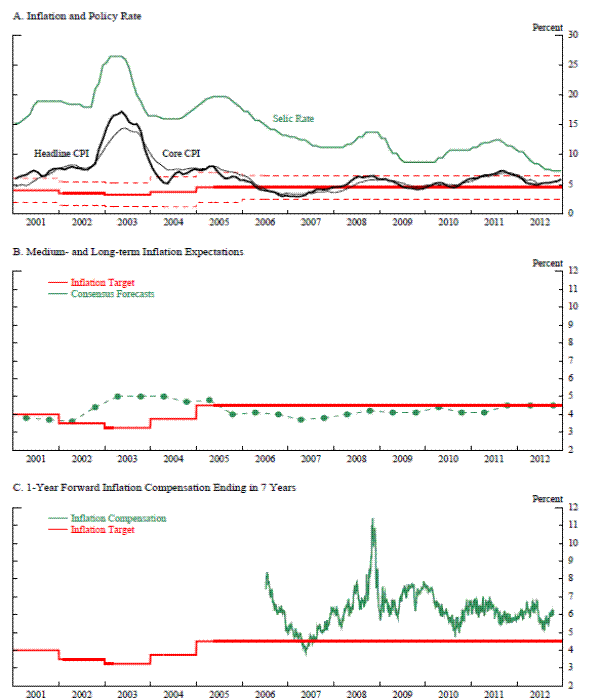
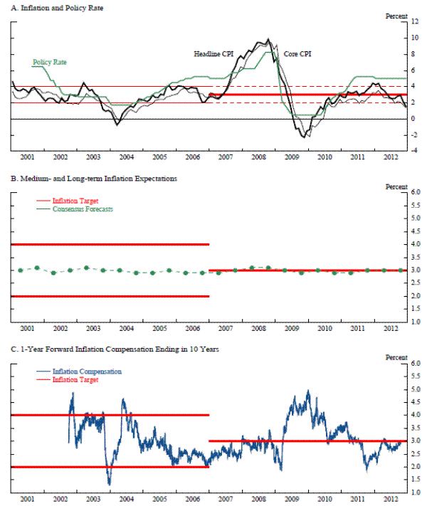
Figure 3: Mexico: Inflation, forward inflation compensation, and survey measures

Figure 4: Zero curve estimation: outstanding bonds and longest-maturity bond

Figure 5: Bond price fitting errors

Figure 6: Zero-coupon yield and inflation compensation estimates

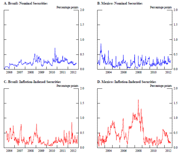
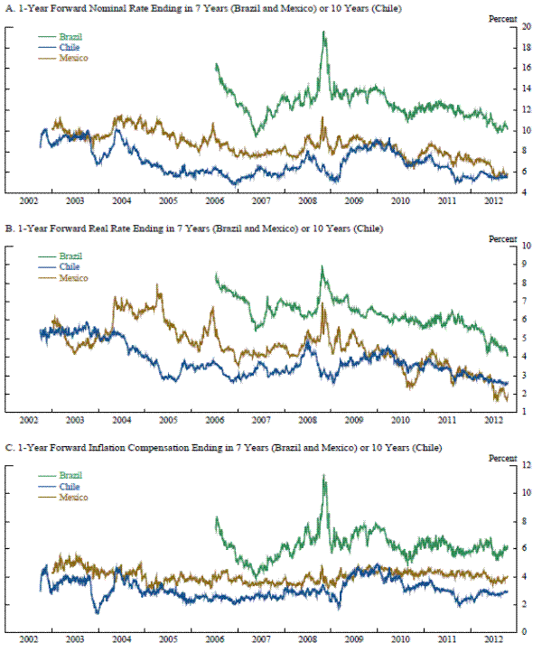
References

Alichi, A., L. Catao, D. Leigh, A. Pescatori, O. Kamenik, H. Kim, D. Laxton, R. Portillo, J. Simon, and F. Zanna (2011),International Monetary Fund, World Economic Outlook (Sepember), Chapter 3 , 101-133.

Andersson, M., L. J. Overby, and S. Sebestyen (2009), Which News Moves the Euro Area Bond Market?,German Economic Review,10, 1-31.

Beechey, M. J., B. K. Johanssen, and A. T. Levin (2011), Are Long-Run Inflation Expectations Achored More Firmly in the Euro Area than in the United States?, American Economic Journal: Macroeconomics,3, 104-129.

Beechey, M. J. and J. H. Wright (2009), The High-Frequency Impact of News on Long-term Yields and Forward Rates: Is it real?, Journal of Monetary Economics, 56, 535-544.

Bevilaqua, A., M. Mesquita, and A. Minella (2007), Brazil: Taming Inflation Expectations, Central Bank of Brazil, Working paper, No. 129.

BIS (2005), Zero-Coupon Yield Curves: Technical Documentation, Bank for International Settlements,Basle.

Capistran, C. and M. Ramos-Francia (2010), Does Inflation Targeting Affect the Dispersion of Inflation Expectations?, Journal of Money, Credit and Banking, 42 , 113-134.

de CarvalhoFilho, I. (2011), 28 Months Later: How Inflation Targeters Outperformed Their Peers in the Great Recession, B.E. Journal of Macroeconomics, 11, Article 22.

Diebold, F. X. and C. Li (2006), Forecasting the Term Structure of Government Bond Yields, Journal of Econometrics, 130, 337-364.

Fraga, A., I. Goldfajn, and A. Minella (2004), Inflation Targeting in Emerging Market Economies, NBER Macroeconomics Annual 2003, Volume 18; eds M. Gertler and K. Rogoff; The MIT Press.

Galati, G., S. Poelhekke, and C. Zhou (2011), Does the Crisis Affect Inflation Expectations?,International Journal of Central Banking, 7, 167-207.

Gurkaynak, R. S., A. T. Levin, A. N. Marder, and E. T. Swanson (2007a), Inflation Targeting and the Anchoring of Inflation Expectations in the Western Hemisphere, Monetary Policy under Inflation Targeting;eds F. Mishkin and K. Schmidt-Hebbel; Central Bank of Chile; Santiago, Chile, 415-465.

Gurkaynak, R. S., A. T. Levin, and E. T. Swanson (2010a), Does Inflation Targeting Anchor Long-Run Inflation Expectations? Evidence from the U.S., U.K., and Sweden, Journal of the European Economic Association,8, 1208-1242.

Gurkaynak, R. S., B. Sack, and E. T. Swanson (2005), The Sensitivity of Long-Term Interest Rates to Economic News: Evidence and Implications for Macroeconomic Models,American Economic Review,95,425-436.

Gurkaynak, R. S., B. Sack, and J. H. Wright (2007b), The U.S. Treasury Yield Curve: 1961 to the Present, Journal of Monetary Economics, 54, 2291-2304.

Gurkaynak, R. S., B. Sack, and J. H. Wright (2010b), The TIPS Yield Curve and Inflation Compensation, American Economic Journal: Macroeconomics,2, 70-92.

Hammond, G. (2012), State of the Art of Inflation Targeting, Centre for Central Banking Studies, Handbook- No. 29, Bank of England.

Hordahl, P. (2009), Disentangling the Drivers of Recent Shifts in Break-Even Inflation Rates, Bank of International Settlements Quarterly Review, March, 10-11.

J. P. Morgan (2006), Local Markets Guide, March 2006.

J. P. Morgan (2012), Local Markets Guide, Septmber 2012.

Levin, A. T., F. M. Natalucci, and J. M. Piger (2004), The Macroeconomic Effects of Inflation Targeting, Federal Reserve Bank of St. Louis Review, 86, 51-80.

Mishkin, F. S. and K. Schmidt-Hebbel (2007), Does Inflation Targeting Make a Difference?, NBER Working Paper, No. 12876.

Nelson, C. R. and A. F. Siegel (1987), Parsimonious Modeling Of Yield Curves, Journal of Business,60, 473-489.

Novo, A. (2004), Meirelles defende a independencia do BC,Correio Braziliense, January 18.

Radowitz, B. (2007), Brazil Real Closes Weaker On Govt's Inflation-Target Decision, Dow Jones International News, June 26.

Ranos-Francia, M. and A. T. Garcia (2005), Reducing Inflation Through Inflation Targeting: The Mexican Experience,Bank of Mexico Working paper, No. 2005-01.

Spiegel, M. (1998), Central Bank Independence and Inflation Expectations: Evidence from British Index- Linked Gilts, Federal Reserve Bank of San Francisco Economic Review,1, 3-14.

Svensson, L. E. O. (1994), Estimating and Interpreting Forward Interest Rates: Sweden 1992-1994, NBER Working Paper Series, 4871.

Svensson, L. E. O. (1999), Inflation Targeting: Some Extensions, Scandinavian Journal of Economics, 101, 337-361.

Gazeta Mercantil (2007), Finance minister defends 4.5% inflation target.,June 22.

Tombini, A. and S. Lago Alves (2006), The Recent Brazilian Disinflation Process and its Costs,Central Bank of Brazil, Working paper, No. 109.

Valdes, R. (2007), Inflation Targeting in Chile: Experience and Selected Issues, Central Bank of Chile,Economic policy paper, No. 22.

Footnotes

* We thank seminar participants at the Federal Reserve Board and the Risk & Return Brazil 2012 Conference for helpful comments. The views expressed in this paper are solely the responsibility of the authors and should not be interpreted as reflecting the views of the Board of Governors of the Federal Reserve System or of any other employee of the Federal Reserve System. Return to Text

* Corresponding author. Board of Governors of the Federal Reserve System, Washington, D.C. 20551, US. Tel.: (202) 452-2359. E-mail addresses: [email protected] (M. De Pooter), [email protected] (P. Robitaille), [email protected] (I. Walker), [email protected] (Michael Zdinak) Return to Text

1. According to Hammond (2012), 27 countries are considered to have inflation targeting frameworks: Armenia, Australia, Brazil, Canada Chile, Colombia, the Czech Republic, Ghana, Guatemala, Hungary, Indonesia, Iceland, Israel, Korea, Mexico, New Zealand, Peru, the Philippines, Poland, Romania, Serbia, South Africa, Sweden, Thailand, and Turkey, and the United Kingdom. Return to Text

2. See, for example, Mishkin and Schmidt-Hebbel (2007). de Car valho Filho (2011) finds that countries with inflation targeting regimes experienced lower output loss during the recession that followed the global financial crisis of 2008, even after taking into account other potential drivers of economic performance. But countries that have adopted inflation targeting tend to be the ones that have also undertaken other economic reforms. Return to Text

3. The Bank of Mexico, for example, took several steps to improve its communications with the public. In 2007, the Bank of Mexico began to publish its inflation forecasts and in January 2011 began to release the minutes to its monetary policy meetings. Return to Text

4. Besides reflecting these two factors, Hordahl (2009) notes that inflation compensation also reflects liquidity premia and "technical" market factors, both of which we consider below and which we control for in our regression analysis in Section 4.1 Return to Text

5. Alichiet al., (2011), for example, use survey measures and find that long-term inflation expectations in inflation-targeting emerging market economies are less sensitive to changes in short-term inflation expectations than are countries with alternative monetary arrangements. They follow the methodology in Levin, Natalucci, and Piger (2004), who used survey measures but only considered developed economies. Return to Text

6. Whether this result has held up since the onset of the European fiscal crisis remains an open question. Return to Text

7. Brazil is an exception as the Central Bank of Brazil conducts a long-horizon survey that is updated on a weekly basis. Return to Text

8. See also Spiegel (1998). Return to Text

9. Chile's government had been setting annual inflation targets since the early 1990s a "fully fledged" inflation target was adopted in 1999, when the central bank abandoned its heavily managed exchange rate policy. Return to Text

10. On Brazil's experiences under inflation targeting, see Fraga, Goldfajn, and Minella (2004), Tombini and Lago Alves (2006), Bevilaqua, Mesquita, and Minella (2007). On Mexico's experiences, see Ranos-Francia and Garcia (2005). On Chile's experiences, see Valdes (2007). Return to Text

11. The chart shows only the medium-term inflation target, that is, the target that is announced a year and a half in advance. Between 2002 and 2003, the government raised the target in response to a rise in inflationary pressures, and in [2003 and 2004], the central bank announced adjusted inflation targets in which it specified the extent to which it would accommodate adverse shocks. These adjusted targets should be viewed as higher upper limits of tolerance range rather than higher a long-term inflation target, that is, the desired level of steady state inflation. Return to Text

12. The inflation target is decided by the central bank in consultation with the government. In mid-2004, then-Central Bank governor Henrique Meirelles stated that "[w]e are making for 2005 and 2006 a smooth transition for [an inflation] target of 4 percent, which is the long-term goal..." Novo (2004), translation is ours). However, then-Finance Minister Antonio Palocci, left office in 2005, and press reports suggest that his successor and current finance minister, Guido Mantega, preferred that the inflation target remain at 4½ percent. Press reports have noted that Meirelles preferred a 4 percent inflation target. See Radowitz (2007)>, Nunes (2007) and Gazeta Mercantil (2007). In October 2012, Central Bank President Alexandre Tombini, who assumed the presidency in January 2011, stated that "we have to have the ambition of having inflation converge to [inflation] of our trading partners, as his, in the medium and long-term, would make a difference...(O Estado de São Paulo 2012)." Return to Text

13. They follow the methodology in Levin et al (2004). Return to Text

14. Consensus Forecasts' long-term inflation survey measures for Brazil, Chile and Mexico are released twice a year, in April and October, and reflect respondents' perception of the expected average annual inflation rate between five and ten years out. Return to Text

15. Wright (2009) even go one step further and use high-frequency intraday quotes on U.S. Treasury Inflation Protected Securities and nominal Treasury securities to construct intraday inflation compensation measures. Return to Text

16. In contrast, even some developed economies, including for example Canada and Germany, still have much less developed inflation-linked bond markets with only a small number of bonds outstanding at any given time. This greatly complicates, or even makes it impossible, to estimate reliable real zero coupon curves for these countries. Return to Text

17. For example, the Bank of International Settlements, BIS (2005), reports that nine out of the thirteen (predominantly European) central banks which report their zero coupon curve estimates to the BIS use either the Nelson and Siegel (1987) model or an extension of it, the Svensson (1994) model, to construct zero-coupon yield curves. Return to Text

18. This restriction on the model-implied instantaneous short rate turns out to work well as we were able to eliminate the occasional odd yield curves that resulted when not imposing the short rate restriction. Return to Text

19. See https://mm.jpmorgan.com/ Return to Text

20. See https://www.precios.com.mx/ Return to Text

21. Gurkaynak, Sack and Wright (2007b) show that for estimating zero coupon curves from U.S. Treasury bonds, one needs the Svensson (1994) model to accurately fit bond prices in the very longest end of the curve. However, the Svensson model requires estimating additional parameters compared to the Nelson-Siegel model. Therefore, due to the relatively small number of bond prices that we have available for each day, we only consider maturities of up to fifteen years. In practice, only a few very long-maturity bonds have been issued in Brazil, Chile, and Mexico and imposing this restriction never removes more than one or two bonds. Return to Text

22. Because the Nelson-Siegel model is a four-parameter model, we can only construct zero coupon curves on days where at least four bond prices are available. Return to Text

23. J.P. Morgan reports (see J.P. Morgan (2006, 2012), that liquidity in Mexican bond markets has improved over time, stating that the liquidity in 10-year Mexican bonds has "increased markedly", with bid-ask spreads having fallen and foreign holdings having risen from 18% in early 2006 to about 60% in August 2012. Return to Text

24. While many emerging market countries experienced a sudden stop as investors fled to safety following the bankruptcy of Lehman Brothers in September 2008, Brazil and Mexico experienced an additional source of instability when it was revealed that firms in both countries, including several large ones such as Aracruz Celulose SA in Brazil and CEMEX and Gruma in Mexico, were found to have had unhedged dollar liabilities. Return to Text

25. While the longest maturity that is consistently available for Mexico is eight years, we chose the same 7-year maximum maturity out of convenience. While studies that have examined far-forward inflation compensation for developed economies typically look at 1-year forward rates ending in 10 years, our 1-year forward rates ending in 7 years are still far enough in the future such that unforeseen shocks to prices and the real economy should not drive inflation away from the target if inflation expectations are well-anchored. Return to Text

26. See www.riskamerica.com Return to Text

27. Chile has had inflation-indexed bonds outstanding for decades. Return to Text

28. Gurkaynak, Levin, Marder (2007a) show this point in their Figure 5B. Return to Text

29. Gurkaynak, Levin, Marder (2007a) also study inflation compensation in Chile and find that these do not react significantly to Chilean and U.S. news surprises. However, due to data limitations, they only analyzed the relatively short sample from August 2002 to October 2005. Furthermore, their set of news surprises was small and, as the authors note, the survey measures used were likely to be somewhat stale. Here we use a much longer time series of inflation compensation, as well as a larger set of economic news surprises (see Section

)index Return to Text

30. Recall that we use n = 7 for Brazil and Mexico, while for Chile n=10. Return to Text

31. As noted by Galati,Poelhekke, and Zhou (2011), because inflation compensation is defined at the difference between nominal and real (forward) rates, we already filter out most of the impact of liquidity and technical factors, provided that these affect nominal and real bond prices in a similar way. Return to Text

... rate,³²

33. Instead of Markit Group's PMI, for Mexico we instead include the business climate index produced by the Mexican Institute of Finance Executives (IMEF). Return to Text

34. To construct survey expectations for economic data releases, Bloomberg initially asks respondents to input their forecasts two weeks prior to the actual release. Respondents can then submit their forecast, or change their previously submitted forecast up until roughly one hour before the release time of the announcement. Return to Text

35. We run the regressions including only the days with one or more surprises. Regression results when we included all days (which entails including a substantial number of days with zero values for surprises) were very similar. Return to Text

36. It turns out to matter little for the results whether we include the fourth quarter of 2008 or not. However, as shown in Figure 6, the inflation compensation do exhibit an outlier-level amount of volatility for those months. Return to Text

37. Instead of incorporating surprises in the policy rate directly, we also used the daily change in the 3-month Treasury Bill rate which some authors have claimed is a better measure of monetary policy surprises. The results were virtually the same. Return to Text

38. For Chile, this corroborates the conclusion of Gurkaynak et al (2007a). Return to Text

39. Over 80% of Mexico's trade is with the U.S. Return to Text

40. A more sophisticated subsample analysis, for example using rolling windows and testing for breaks as in Galati et al (2001) could shed more light on the anchoring of inflation expectations over time. However, we do not address this here and leave this for further research. Return to Text

^♣ This version is optimized for use by screen readers. Descriptions for all mathematical expressions are provided in LaTex format. A printable pdf version is available. Return to Text