Skip to: [Printable Version (PDF)] [Bibliography] [Footnotes]

System Committee on International Economic Analysis: Screen Reader version ^♣

Diversification, Cost Structure, and the Stock Returns of Multinational Corporations^*

José L. Fillat**

Federal Reserve Bank of Boston

Stefania Garetto*

Boston University

Lindsay Oldenski*

Georgetown University

April 28, 2013

Very Preliminary

Abstract:

This paper investigates theoretically and empirically the relationship between the geographic structure of a multinational corporation and its stock market returns. We use a structural model to identify two main channels through which the fact of being a multinational firm affects returns. On the one hand, multinational activity offers diversification potential. On the other hand, there is cash flow risk arising from hysteresis and potential losses induced by sunk entry costs and fixed costs. To identify these channels empirically, we merge Compustat/CRSP data on stock returns with the Bureau of Economic Analysis data on the operations of multinational corporations. Preliminary empirical results confirm the predictions of the theory.
Keywords: Multinational firms, diversification, risk premium, stock returns.
JEL Classification: F14, F23, G12.

1 Introduction

An extensive literature in finance has been investigating cross-sectional differences in stock returns across firms, assets, or portfolios, identifying several variables driving returns differentials.¹ However, existing explanations of the cross section of returns overlooked the role of the international status of the firm. About half of the manufacturing firms publicly listed in the U.S. are multinational corporations, with assets, operations, and sales in many countries. The objective of this paper is to investigate whether the geographic structure of a multinational corporation affects its stock market returns.

We present a streamlined, multi-country version of the model developed by Fillat and Garetto (2012) to identify two main channels via which the fact of being a multinational firm affects returns. On the one hand, multinational activity offers diversification potential: if the business cycles of two countries are not perfectly correlated, multinational sales diversify away the risk arising from country-specific fluctuations and reduce equilibrium returns. This mechanism, referred to as the "diversification channel", implies that, in equilibrium, MNCs should exhibit lower returns than non-multinational firms - all else equal. Within multinationals, returns should be higher for those firms operating in countries whose business cycles are more correlated with each other. On the other hand, there is risk arising from hysteresis and potential losses induced by sunk entry costs and fixed costs: firms open affiliates abroad when prospects of growth make foreign operations profitable, but they must bear sunk entry costs to open an affiliate, and fixed costs of production. If the host country is hit by a negative shock, the affiliate may incur losses. The parent may find optimal not to exit the foreign market and bear those losses for a while, in order not to forego the sunk cost it paid to enter. The higher the fixed and sunk costs of production, the higher the potential losses and the longer the time for which a firm is willing to bear them. These potential losses are perceived as a cash flow risk by the investors, who must be rewarded by expected stock returns that are higher the higher the fixed and sunk costs of production. This second mechanism, that we refer to as the "sunk cost channel", implies that MNCs with affiliates in countries where entry is more costly and fixed operating costs are higher should exhibit higher stock returns than MNCs with affiliates located in countries that are more easily and cheaply accessible.

The question of understanding why and how average stock returns vary across firms based on certain characteristics is central to the asset pricing literature. Nonetheless, existing empirical work on the returns of multinational corporations is scarce. Early research examined the returns of MNCs to assess whether firms' foreign activities provide diversification benefits to their stockholders. Support for this "diversification hypothesis" is scarce: Jacquillat and Solnik (1978) regressed the returns of multinationals from nine countries on a set of market indices and found that multinational returns tended to covary most with the firm's home market, hence not providing any evidence in support of diversification. Senchack and Beedles (1980) compared the risk, returns and betas of portfolios of multinationals with portfolios of domestic and international equities and found that multinationals did not deliver diversification benefits. Using a different methodology based on mean-variance spanning tests, Rowland and Tesar (2004) also found limited evidence of diversification benefits for MNCs. More recently, using a sample of manufacturing firms from Compustat, Fillat and Garetto (2012) have shown that the stock market returns of multinational corporations (henceforth, MNCs) are systematically higher than the stock market returns of non-multinational firms, also against what would be predicted by the diversification hypothesis. The structural model in their paper sheds light on this "puzzle" by introducing another channel, the sunk cost channel, that increases the risk to which MNCs are exposes compared to non-multinational firms and can potentially explain MNCs' higher returns and the lack of evidence of diversification.

The scarcity of firm-level geographic information in the Compustat Segments database prevented Fillat and Garetto (2012)'s analysis from studying cross-sectional variation in returns across multinational corporations differing in their geographical organization. By merging Compustat/CRSP data on stock returns with the Bureau of Economic Analysis (BEA) data on the operations of multinational corporations, in this paper we are able to study the relationship between firms' multinational organization and stock returns. The data display a large amount of variation across MNCs' operations in foreign markets in terms of number and characteristics of countries entered, number of affiliates (total and per country), volume of foreign sales, and employment (total, per country, and at the affiliate level). The results of our regression analysis are consistent with the predictions of the model in showing that GDP growth correlations and entry costs in the countries in which these firms have affiliates are correlated with the returns that they offer in the stock market.

Our empirical analysis starts with a reduced form specification whose goal is to explore the statistical relationship between GDP growth correlations, entry costs, and returns. In this specification we proxy entry costs with country level data on the cost of starting a business from the World Bank's Doing Business database. The results of our baseline regressions neglect the impact that potential foreign activities in countries other than the ones currently served have on the value of the firm and hence on its returns (the option value). To control for the contribution of the option value to stock returns, we also present the results of a two-stage approach. In the first stage, we estimate the probability that each firm will have an affiliate in each country using standard predictors of FDI activity. In the second stage, we estimate the impact of the characteristics of countries in which the firm has affiliates on annual returns, controlling for characteristics of the countries where the firm does not have any affiliates.

The results of the reduced form analysis are useful to illustrate the importance of GDP growth correlations and sunk costs for the firms' returns, but the estimated parameters do not have a structural interpretation. For this reason, we also run regressions based on the structural equation that the model delivers, linking returns to a function of the GDP growth correlations and of the elasticity of firm value with respect to GDP. The results of this specification allow us to do two things. First, by looking only at those firms that have affiliates in only one country, we can compare each country' contribution to the risk premium. Second, using the entire sample of firms, we can separate the contribution of option value versus assets in place in explaining stock returns.

This paper aims to deepen our understanding of the operations of multinational corporations by examining the relationship between their geographical structure and their stock market returns. As such, our analysis is related to empirical research using the BEA data on the operations of multinational corporations, starting with Kravis and Lipsey (1982) and Brainard (1997), and more recently Yeaple (2003), Helpman, Melitz, and Yeaple (2004), and Yeaple (2009). We contribute to this literature by providing more information on the operations of MNCs from a financial markets perspective.² The theoretical framework at the basis of our empirical specifications builds on the literature on investment under uncertainty, particularly on the real option value framework developed by Dixit (1989) and Dixit and Pindyck (1994) as applied to the heterogeneous firms framework by Fillat and Garetto (2012).

Our work is also related to a strand of literature in corporate finance that studies the linkages between international activity and stock market variables. Denis, Denis, and Yost (2002) find that multinational corporations trade at a discount, and Baker, Foley, and Wurgler (2009) link empirically market valuations, returns, and FDI activity. Our analysis departs from these contributions by taking into account the full geographic structure of the firm as a determinant of stock returns, and by starting from the predictions of a structural model to identify the economic forces that link MNCs' structure and stock returns in the data.

The rest of the paper is organized as follows. Section 2 lays out the theoretical model at the basis of our empirical specification. Section 3 describes the financial data and the data on the operations of multinational corporations. Section 4 presents our baseline empirical specification and results. Section 5 outlines the next steps of the analysis, and Section 6 concludes.

2 The Returns of Multinational Corporations

The model we develop in this section is designed to illustrate how the stock returns of multinational corporations depend on a set of variables related to their international activities across countries. At the aggregate level, the model is specified as an endowment economy, consistently with consumption-based asset pricing models. We take aggregate consumption as given, and focus on modeling the production side of the economy, where firms' valuations are affected by firm-level and country-level characteristics. Firms' valuations and the covariance of their profits with the agents' stochastic discount factor drive the returns.

The model is a multi-country extension of the framework developed in Fillat and Garetoo (2012).³ The economy is composed by countries: a Home country, that we denote by , and potentially asymmetric foreign countries, that we denote by . Time is continuous. Each country is hit by aggregate shocks to its GDP growth rate, which are described by the following geometric Brownian motions:

$\begin{displaymath}\frac{dY_i}{Y_i} = \mu_i dt + \sigma_i dz_i, ~{\rm for}~ i=h,j ~{\rm and}~ j=1,...N \end{displaymath}$

(1)

where $\mu_i \geq 0$ , $\sigma_i>0$ .

denotes the GDP level in country

and

is the increment of a standard Wiener process. GDP growth processes may be correlated across countries: let $\rho_j \in [-1,1]$ denote the correlation between the GDP growth of the Home country and the one of country

International markets are incomplete: aggregate consumption in each country is equal to the GDP level , and there is no possibility of consumption smoothing over time. We assume complete home bias in the asset markets, in the sense that firms are owned by agents in country , who discount cash flows with the following discount factor :⁴

$\begin{displaymath}\frac{dM_h}{M_h} = -r_h dt - \gamma\sigma_h dz_h \end{displaymath}$

(2)

where

denotes the risk-free rate in the Home country and $\gamma$ denotes risk-aversion.⁵

Let ${\cal V }$ denote the value of a multinational firm. The value of a firm depends on both firm-specific characteristics, like productivity, size, employment, etc., and on country-specific characteristics, like the GDP growth processes of the countries where it operates, entry costs, and other operating costs. For this reason, we write ${\cal V}= {\cal V} (a,\bar{Y},\bar{X})$ , where denotes firm-specific characteristics, $\bar{Y} = (Y_h, Y_1,... Y_N)$ denotes a vector whose entries are the realizations of the GDP described by (1), and $\bar{X} = (X_h, X_1,... X_N)$ denotes a vector whose entries are other country-specific characteristics affecting firm value. Consistently with the literature on selection into export and multinational activity and with the empirical evidence on firms' international dynamics, fixed operating costs of production and sunk costs of entry into a market are particularly relevant among the variables entering the vector $\bar{X}$ .⁶

We assume that firms' activities are independent across countries, i.e. each firm makes entry and production decisions country-by-country.⁷ Since the decision of setting up a foreign affiliate is endogenous and affected by uncertainty through the country-specific GDP growth shocks, we must consider the fact that a firm's valuation is affected both by its assets currently in place in various countries, and by the possibility of entering new countries (its option value).⁸ For these reasons we write the value of the firm as:

$\begin{displaymath}{\cal V} (a,\bar{Y},\bar{X}) = V_h (a,Y_h,X_h) + \sum_{j\in {\cal A}} V_j(a,Y_j,X_j) + \sum_{j\not\in{\cal A}} V^o_j(a,Y_j,X_j) \end{displaymath}$

(3)

where

denotes the firm's value of domestic sales,

denotes the value of the firm's affiliate sales in country

if the firm has an affiliate there, and

denotes the option value of the firm's affiliate sales in country

if the firm does not have an affiliate there. ${\cal A}$ denotes the set of countries where the firm has affiliates ( ${\cal A} \subseteq \{1,2,...N\}$ ).

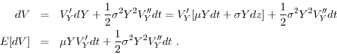
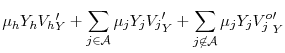
Given that we do not observe exit in our sample, we assume that all firms sell in the Home country. Conversely, firms' entry and exit into foreign markets are endogenous and observable. For these reasons, over a generic time interval $\Delta t$ we can express the components of a firm's value function as:

$\displaystyle V_h(a,Y_h,X_h)$	$\textstyle =$	$\displaystyle \pi_h(a,Y_h,X_h) M\Delta t + E[M\Delta t \cdot V_h (a,Y'_h,X_h\vert Y_h)]$	(4)
$\displaystyle V_j(a,Y_j,X_j)$	$\textstyle =$	$\displaystyle \max\left\{\pi_j(a,Y_j,X_j) M\Delta t + E[M\Delta t \cdot V_j (a,Y'_j,X_j\vert Y_j)] ~;~ V_j^o(a,Y_j,X_j) \right\}$	(5)
$\displaystyle V_j^o(a,Y_j,X_j)$	$\textstyle =$	$\displaystyle \max\left\{ E[M\Delta t \cdot V_j^o (a,Y'_j,X_j\vert Y_j)] ~;~ V_j(a,Y_j,X_j) - F_j \right\}$	(6)

where $\pi_i(a,Y_i,X_i)$ denotes the flow profits of the firm in country

(for

and

denotes the sunk entry cost that a firm has to cover to open an affiliate in country

, and the terms in expectations indicate the firm's continuation value in the event in which its status in a country does not change (i.e. it does not enter or exit the country).

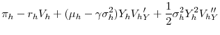
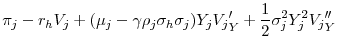
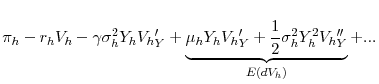
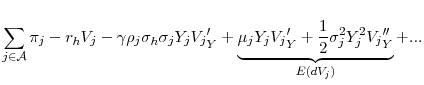
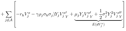
We show in the Appendix that, in the continuation regions, the three value functions above satisfy the following no-arbitrage conditions:

$$\displaystyle \pi_h - r_h V_h + (\mu_h -\gamma\sigma_h^2 )Y_h {V_h}_Y' dt + \frac{1}{2} \sigma_h^2 Y_h^2 {V_h}_Y$	$\textstyle =$	$\displaystyle 0$	(7)
$$\displaystyle \pi_j - r_h V_j + (\mu_j -\gamma\rho_j\sigma_h\sigma_j)Y_j {V_j}_Y' dt + \frac{1}{2} \sigma_j^2 Y_j^2 {V_j}_Y$	$\textstyle =$	$\displaystyle 0$	(8)
$$\displaystyle - r_h V^o_j + (\mu_j -\gamma\rho_j\sigma_h\sigma_j)Y_j {V^o_j}_Y' dt + \frac{1}{2} \sigma_j^2 Y_j^2 {V^o_j}_Y$	$\textstyle =$	$\displaystyle 0.$	(9)

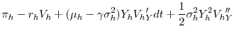
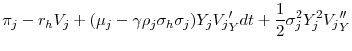
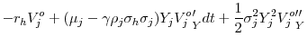
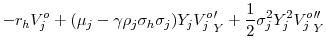
By combining equations (7)-(9) one can obtain the following expression for a multinational's expected returns:⁹

$\begin{displaymath} E(R^f) \equiv \frac{\pi_h + \displaystyle \sum_{j\in {\cal A}}\pi_j + E(d{\cal V})}{{\cal V}}=r_h +\gamma \left( \frac{\sigma_h^2 Y_h {V_h}_Y'}{{\cal V}} + \displaystyle \sum_{j\in {\cal A}} \sigma_h\sigma_j\rho_j \frac{Y_j {V_j}_Y'}{{\cal V}} + \displaystyle \sum_{j\not\in {\cal A}} \sigma_h\sigma_j\rho_j \frac{Y_j{V^o_j}_Y'}{{\cal V}}\right) . \end{displaymath}$

(10)

Equation (10) summarizes the implications of the model for the dependence of returns on country-specific variables, and is the theoretical foundation of our empirical specifications. The risk aversion, $\gamma$ , represents the price of risk for the representative agent, or how much does she need to be rewarded for additional risk incurred by the firms. The terms in the parenthesis capture the three sources of risk that a firm is exposed to: domestic risk, risk from the countries where the firm has an affiliate, and risk from the countries where the firm has the option of opening an affiliate, respectively. The first term of the expression describes the contribution of domestic activities to the returns, and is common to all firms in our sample. The last term captures the option value, which we will address empirically by constructing a proxy in a two-stage model. We now focus on the second term, which we refer to as "assets in place". This term captures the exposure of multinational firms to the risk that emerges from having affiliates in foreign countries, and generates three testable implications.

First, equation (10) indicates that expected returns should be higher the higher the correlations $\rho_j$ between the Home country's GDP growth rate and the GDP growth rates of the host countries. This prediction summarizes the effect of diversification on returns in the model: when the GDP growth rates of two countries are highly correlated, foreign activities provide a relatively small amount of diversification. As a result, MNCs with affiliates in countries whose GDP growth rates are highly correlated with the US GDP growth rate are less diversified (and more risky) than MNCs with affiliates in countries whose GDP growth rates are not strongly correlated with that of the US. Riskier firms command higher returns in equilibrium.

Second, the fact that a firm has activities in a foreign country indicates that the firm paid an entry cost to establish an affiliate there and is bearing fixed operating costs. These costs, which are independent on firm size, affect a firm's value but not its derivative . In other words, the elasticity of the value function is increasing in the fixed and sunk costs of production, and equation (10) indicates that expected returns should be higher the higher the fixed and sunk costs of production in the host countries where it operates. The economic intuition behind this prediction is the following: due to sunk entry costs and fixed costs of production, if a host country is hit by a negative shock, the foreign affiliate of a multinational firm may incur losses. The parent may find optimal not to exit the foreign market and bear those losses for a while, in order not to forego the sunk cost it payed to enter. The extent and duration of these losses are positively correlated with the size of fixed and sunk costs. Investors perceive as a risk the possibility of losses, and this cash flow risk must be rewarded by a higher stock return in equilibrium.

Third, the extensive margin of the number of countries in which a firm operates (the cardinality of ${\cal A}$ ) also matters for the returns. The effect of the number of countries on the returns is ambiguous: on the one hand, operating in more markets may induce more diversification, and then command lower returns in equilibrium. On the other hand, operating in more markets entails paying more fixed and sunk costs, and then a higher risk induced by potential losses. It is a quantitative question to determine which effect is stronger empirically. However, once one controls for country characteristics like the GDP growth correlations and the fixed and sunk costs mentioned above, the number of countries with affiliates should act as a pure extensive margin and increase the firm's riskiness and hence its returns.

The analysis in Section 4 tests the empirical validity of these predictions.

3 Data

To test the predictions of the model outlined in Section 2, we need information on multinational companies' operations across countries and their stock returns. We also need country-level data on GDP growth correlations and on fixed and sunk costs of production.

The Bureau of Economic Analysis collects firm-level data on U.S. multinational company operations in its annual surveys of U.S. direct investment abroad. All U.S. headquartered firms that have at least one foreign affiliate and meet a minimum size threshold are required by law to respond to these surveys. The data include detailed information on the firms' operations both in the U.S. and at their foreign affiliates. To test the predictions of our model, we use information from the BEA data on the countries in which each firm has operations. We also use data on the sales by each foreign affiliate, as well as total global sales by the MNCs to control for the scale of operations in each location and by each firm. The BEA surveys cover both manufacturing and service industries, classified according to BEA versions of 3-digit SIC codes. We include firms in all industries and use data from 1987 through 2009.

Stock market returns data are obtained from the Center for Research in Security Prices (CRSP), which includes information on all firms that are publicly traded in the U.S. stock market.¹⁰ We match the firm level stock return data from CRSP with the firm level data on multinational operations from the BEA to obtain a set of publicly traded US-headquartered multinational firms. To ensure that outlier firms are not biasing our results, we drop observations that fall into the highest or lowest 5 percent in terms of their annual stock market returns. The result is a sample of more than 3200 multinational firms operating in 118 countries and 148 industries over the 23 year period.

There are two components of the risk premium (expected returns in excess of the risk free rate) in equation (10) that emerge from exposure to foreign countries where the firm has affiliates: the covariance with the GDP of the foreign country, and the elasticity of the firm's value with respect to foreign GDP changes. To measure the first component at the firm level, we created a measure, $\rho_{ft}$ , of the extent to which GDP growth in each host country of firm is correlated with GDP growth in the home country (the US). We begin with data on real GDP growth rates by country from the IMF. We assume that expected GDP growth is constant. We then take the correlation between annual U.S. GDP growth and annual GDP growth in each country over our sample period (1987-2009), resulting in a time-invariant GDP growth correlation measure for each country $\rho_j$ . We use these measures together with information on firm 's affiliate sales to construct a firm-level measure of weighted correlation for each firm with affiliates in countries in each year :¹¹

$\begin{displaymath} \rho_{ft} = \sum_{j\in {\cal A}_f} s_{fjt}\rho_j \end{displaymath}$

(11)

where $\rho_j$ is the country-level GDP growth correlation and $s_{fjt}$ is the share of sales by foreign affiliates of firm

that were produced in country

in year

. In other words, the firm-level variable is a weighted average of the GDP growth correlation measures for the countries in which the firm has foreign affiliates, where the share of sales by the affiliates in each country are used as weights.

The second component of risk exposure to foreign countries is the elasticity of the value of the firm with respect to foreign GDP changes, which is a function of firm-level productivity and of the fixed and sunk costs of production. To capture the effect of fixed and sunk cost of opening a foreign affiliate, we use country level data on the cost of starting a business from the World Bank's Doing Business database. Doing Business records all procedures officially required, or commonly done in practice, for an entrepreneur to start up and formally operate an industrial or commercial business. These procedures include obtaining all necessary licenses and permits and completing any required notifications, verifications or inscriptions for the company and employees with relevant authorities. The information used to construct these data comes from official laws, regulations and publicly available information on business entry, and the data are verified in consultation with local incorporation lawyers, notaries and government officials. Our primary specification uses the number of required procedures, however for robustness checks we also use the required number of days and cost to complete these procedures and the paid-in minimum capital requirement. We use these variables to construct a firm-level measure of sunk costs. As with the GDP growth correlations, the firm-level sunk cost variable is a weighted average of the doing business measures for the countries in which the firm has foreign affiliates, where the share of sales by the affiliates in each country are used as weights:

$\begin{displaymath} P_{ft} = \sum_{j\in {\cal A}_f} s_{fjt}P_{j} \end{displaymath}$

(12)

where

is the number of required procedures to start a business in country

Table 1: Summary Statistics

	N. Obs	Mean	Std. Dev.	Min	Max
Annual Returns	23870	0.106	0.343	-0.574	1.095
Market cap ($b)	23870	5.504	20.356	0.001	491.105
Tot. firm sales ($b)	23847	5.275	18.800	(Confidential)	(confidential)
Tot. affiliate sales by firm ($b))	23867	1.904	10.500	(confidential)	(confidential)
N. of affiliates	23870	17.242	42.294	(confidential)	(confidential)
N. of countries	23870	9.445	12.497	(confidential)	(confidential)
Correlation ( $\rho_{ft}$ )	23867	0.630	0.212	-0.355	0.918
Procedures ( $P_{ft}$ )	23867	5.273	2.609	0	17

Table 1 provides summary statistics for the firms in our dataset. The average firm in our sample has about 17 foreign affiliates located in 9 different countries with total global sales of 5.3 billion and a 10.6 percent annual stock market return. The countries these firms operate in require an average of 5 procedures in order to open a new business. The average correlation between the GDP growth in the U.S. and in the host countries is about 0.63.

4 The Role of Diversification and Cost Structure: Empirical Results

4.1 Reduced-Form Analysis

The empirical analysis in this section tests the predictions of the model described in Section 2. The goal of the reduced form specification is to establish a statistical relationship between firm-level stock returns and the relevant explanatory variables that are suggested by the model: GDP growth correlations across countries and fixed and sunk costs of production. Our baseline specification is given by:

$\begin{displaymath} Ret_{ft}= \alpha + \beta_1 \rho_{ft} + \beta_2 P_{ft} + \beta_3 X_{ft} + \delta_{k} + \varepsilon_{ft} \end{displaymath}$

(13)

where $Ret_{ft}$ is the annual stock return of firm

in year

, $\rho_{ft}$ is the weighted correlation of GDP growth between the U.S. and the countries in which firm

has affiliates, and $P_{ft}$ is the weighted average number of procedures required to start a business in the countries in which firm

has affiliates. $X_{ft}$ is a vector of firm level controls, including the total sales of the firm and the number of countries in which it has affiliates. Because the industry in which a firm operates is likely to impact returns by affecting risk and other factors, we also include fixed effects, $\delta_{k}$ , for each firm's primary industry. $\varepsilon_{ft}$ is an orthogonal error term.

Table 2 shows the results. We begin by adding the two variables $\rho_{ft}$ and $P_{ft}$ separately. Column I shows the result of regressing returns on the correlations variable. As predicted, the coefficient on the variable measuring how correlated shocks are between the U.S. and the countries in which a firm operates, $\rho_{ft}$ , is positive and significant. This implies that stock returns are higher (lower) for MNCs with affiliates in countries where GDP growth is more (less) positively correlated with growth in the US. Quantitatively, the interpretation is as follows: ceteris paribus, a firm that engages for the first time in FDI in a destination country whose GDP is perfectly correlated with the domestic GDP would increase its risk premium by $2.7\%$ with respect to a firm engaging in FDI in a country with uncorrelated GDP. This result supports the model in which more highly correlated shocks imply greater risk, and thus higher returns are necessary to compensate for this risk. Column II shows the results controlling for the total global sales of the firm. Total sales capture the scale of firm activity, and have also been shown to be highly correlated with other factors, such as productivity, that may affect returns. The impact of the correlation of GDP growth on stock returns still holds when controlling for total firm sales.

Table 2: The relationship between annual returns, GDP growth correlations, and sunk costs.

	I	II	III	IV	V
correlation ( $\rho_{ft}$ )	0.027***	0.026***			0.034***
correlation ( $\rho_{ft}$ ):Standard Errors	(0.010)	(0.010)			(0.010)
procedures ( $P_{ft}$ )			0.002**	0.002**	0.002**
procedures ( $P_{ft}$ ): Standard Errors			(0.001)	(0.001)	(0.001)
sales		0.008		-0.007	-0.225
sales: Standard Errors		(0.128)		(0.128)	(0.145)
nr of countries					0.001***
nr of countries: standard errors					(0.0002)
Industry FE	YES	YES	YES	YES	YES
N	23742	23719	23745	23722	23719
R-sq	0.0003	0.0003	0.0002	0.0002	0.0011

Notes: *,** and *** indicate significance at the 10, 5 and 1 percent levels, respectively. Robust standard errors, clustered at the firm level, are in parentheses.

Columns III and IV of Table 2 show the results of regressing returns on our proxy for the entry costs. As predicted, the coefficient on the measure of sunk costs, $P_{ft}$ , is positive and significant. As the model predicts, higher sunk costs increase the likelihood that a firm will be willing to bear temporary losses when hit with a negative shock. In particular, returns increase by $0.2\%$ for each additional procedure required in each country of destination. This additional procedure, which proxies sunk and fixed operating costs, increases the risk of experiencing negative cash-flows, and higher returns are necessary to compensate for this risk. Since the average number of business procedures required to open an affiliate in a country is 5, on average, the risk premium generated by entry costs is about 1%. Notice also that the positive and significant coefficient is unchanged when controlling for the total sales of the firm (see Column IV).

Column V of Table 2 controls for both the correlation of GDP growth and our proxy for sunk costs. The results for these measures still hold when both are included. The specification in Column V also includes the number of countries in which a firm operates as a control. As explained in Section 2, the sign of the relationship between the number of countries in which a firm operates and its stock returns is ambiguous. The number of countries in which a firm has affiliates can impact returns through two opposing channels. The risk diversification channel suggests that operating in a larger number of countries will spread risk and thus lead to lower returns. However, the sunk cost channel moves in the opposite direction. Each affiliate that the firm opens in a new country requires additional sunk costs, and these sunk costs make the firm more likely to tolerate temporary losses, increasing risk and raising the returns required to compensate for this risk. Once one controls for the relevant country-level characteristics (like the GDP growth correlations and the fixed and sunk costs mentioned above), the number of countries served should act as a pure extensive margin and increase the firm's riskiness and hence its returns. The positive coefficient on the number of countries confirms the validity of this prediction.

The results displayed in Table 2 are preliminary: the regressions do not control for a set of other variables that have been shown to affect firm-level stock returns, most notably the exposure to aggregate returns on the market portfolio (according to the CAPM model) and measures of leverage (see Cochrane (2001)). Nonetheless, our results confirm the importance of cross-country GDP growth correlations and entry costs into the host countries for the stock returns of US multinationals. These results also disregard the fact that - according to equation (10) - GDP growth correlations and entry costs in the countries in which the firm does not have affiliates also matter, through the option value term. The two-stage model that we present in the next section controls for the components of the option value term by building a proxy based on the estimated probabilities that firms open affiliates in given countries.

4.2 Two-Stage Model

In this section we augment our reduced form specification to include a proxy for the option value component of returns. Equation (10) shows that GDP growth correlations and entry costs matter not only for the value of assets in place, in the countries in which firms have affiliates, but also for the option value of entering new countries.¹² The difficulty in measuring the contribution of the effect of these variables on returns through the option value is that we cannot construct firm-level measures like (11) and (12) since firms do not have sales in these countries. In order to proxy for the contribution of correlations and entry costs to the option value of the firm, we use a two-stage approach. In the first stage, we estimate the probability that each firm will have an affiliate in each country using standard predictors of FDI activity. In the second stage, we estimate the impact of the characteristics of countries in which the firm does have affiliates on annual returns, controlling for characteristics of the countries where the firm does not have any affiliates. We use the predicted probability of entering each country from the first stage as weights in constructing these characteristics.

The first stage estimation draws from the literature on the determinants of FDI. According to the knowledge capital model developed by Carr, Markusen, and Maskus (2001) and Markusen and Maskus (2002), the volume of FDI activity between two countries depends on the sum of the GDPs of the countries, the squared difference in their GDPs, the difference in skilled labor endowments, and trade costs. The proximity-concentration model developed by Brainard (1997) and Helpman, Melitz, and Yeaple (2004) suggests that a firm's decision to engage in FDI is a function of proximity, which we proxy with distance, and market size, measured by the sum of U.S. GDP and the GDP of the host country. Table 3 shows the results of a probit model of the likelihood of a given firm having an affiliate in a given country in a given year using these explanatory variables. When considering the possible countries in which a firm may operate, we limited the sample to the top 50 destination countries, which account for 96 percent of all foreign activity by U.S. firms. Consistent with the knowledge capital and proximity-concentration models, each of the explanatory variables is a significant predictor of whether or not a given firm will have an affiliate in a given country.

Table 3: First stage estimation: selection into FDI.

	-0.238***
:Standard Errors	(0.003)
	0.929***
: Standard Errors	(0.005)
	-0.351***
:Standard Errors	(0.002)
	-0.045***
:Standard Errors	(0.001)
	-0.012***
:Standard Errors	(0.005)
N	3113404
Pseudo R-sq	0.027

Notes: Robust standard errors in parentheses. *** indicates significance at the 1 percent level.

For each firm, we use these first stage results to construct a predicted probability of entering each country in which the firm does not currently have an affiliate. We then use these predicted probabilities to construct a weighted average of the correlation between shocks in the U.S. and shocks in the countries in which the firm does not have affiliates, using the probability that the firm would have affiliates in each country as weights.

Using the results of the probit to proxy for the option value is consistent with the model we developed in Section 2. According to the theory, the option value of a firm in a foreign country is higher the likelier a firm is to enter a given country. In the language of the model, a firm enters a country when its expected profits in that country are above some threshold (that one can derive explicitly given functional forms for preferences and technologies). The estimated probability of entering a country that results from the probit can then be interpreted as a measure of how close a firm is to the entry threshold and hence of how important the option value of entering that country is.

The weighted correlation of GDP growth between the U.S. and countries in which the firm does not currently have affiliates is calculated as

$\begin{displaymath} \rho^o_{ft} = \frac{\displaystyle \sum_{j \not\in {\cal A}} prob_{jt}^f\rho_{j}}{\displaystyle \sum_{j \not\in {\cal A}} prob_{jt}^f} \end{displaymath}$

(14)

where $prob_{jt}^f$ is the predicted probability that firm

has an affiliate in country

in time

from the first stage and $\rho_{j}$ is the correlation of GDP growth between the U.S. and country

. We construct a similar measure for the weighted average number of procedures required to start a business in the countries in which the firm does not currently have affiliates.

Table 4: Summary statistics by affiliate presence.

	Correlation	Procedures
Countries with affiliates	0.630	5.273
Countries without affiliates	0.393	7.72

Table 4 shows the weighted average GDP growth correlations and number of procedures required to start a business for the countries in which a firm does and does not have affiliates. For the average firm in our sample, the GDP growth correlation for countries in which the firm has affiliates is 0.63. The weighted correlation of shocks for countries in which they do not have affiliates is 0.39. These numbers suggest that U.S. MNCs don't choose their affiliates' host countries to diversify away risk. If this were the case, we would observe them self-selecting into countries whose GDP growth is less correlated with the U.S. GDP growth. The weighted average number of procedures required to start a business in the countries where the firms have affiliates is 5.3. For countries in which they do not have affiliates, that weighted average is 7.7. These numbers indicate that U.S. MNCs privilege locations with lower entry costs (measured in terms of procedures required to start a business).

Table 5: Second stage estimation: the relationship between annual returns, GDP growth correlations, and sunk costs, controlling for the option value of entering new countries.

	I	II	II	IV	V
correlation ( $\rho_{ft}$ )	0.026***	0.025***			0.033***
correlation ( $\rho_{ft}$ ):Standard Errors	(0.009)	(0.010)			(0.010)
procedures ( $P_{ft}$ )			0.002***	0.002***	0.002***
procedures ( $P_{ft}$ ):Standard Errors			(0.001)	(0.001)	(0.001)
sales		-0.004		0.002	-0.002
sales:standard errors		(0.014)		(0.013)	(0.015)
nr of countries					0.001***
nr of countries: standard errors					(0.0009)
correlation non-affiliates ( $\rho^o_{ft}$ )	-0.057*	-0.060*			0.074
correlation non-affiliates ( $\rho^o_{ft}$ ):standard errors	(0.034)	(0.036)			(0.062)
procedures non-affiliates ( $P^o_{ft}$ )			0.008*	0.008*	0.01
procedures non-affiliates ( $P^o_{ft}$ ):standard errors			(0.005)	(0.005)	(0.007)
Industry FE	YES	YES	YES	YES	YES
N	23611	23589	23614	23592	23589.000
R-Sq	0.0004	0.0004	0.0004	0.0004	0.0012

Notes: Dependent variable is annual stock market returns. *,** and *** indicate significance at the 10, 5 and 1 percent levels, respectively. Robust standard errors are in parentheses.

Table 5 shows the reduced form results controlling for characteristics of the countries in which each firm does not have affiliates. The effects of GDP growth correlations and the number of procedures required to start a business are qualitatively and quantitatively similar to the results from Table 2. Only the magnitude of the coefficient on GDP growth correlations is slightly lower once the option value of countries in which the firm does not currently operate has been controlled for.

The effect of the GDP growth correlations and entry costs on the returns via the option value component should have the same sign as the effect of these forces through the component measuring assets in place. This is true for the number of procedures $P^o_{ft}$ , which exhibit a positive and significant coefficient, but not for the correlations $\rho^o_{ft}$ , whose coefficient is negative and significant. However, both coefficients lose significance when controlling for both total sales of the firm and the number of countries entered.

4.3 Structural Analysis

The regressions we presented above confirm the existence of a statistical relationship linking GDP growth correlations, sunk and fixed costs of production and the stock returns of multinational corporations. We now move to a more structural approach, which is derived closely from the theoretical relationship that the model delivers (equation (10)). The scope of the structural analysis presented here is to assess the goodness of fit of the model, and to quantify the contribution of assets in place versus option value to the expected returns.

We can re-write equation (10) as:

$\begin{displaymath} E(ret^f) = \alpha + \gamma\sigma_h \sum_{j\in {\cal A}} \sigma_j \rho_j \varepsilon_j^f + \eta^f \end{displaymath}$

(15)

where

denotes the expected returns of firm

, $\sigma_j$ is the standard deviation of GDP growth in country

, $\rho_j$ is the correlation of GDP growth between the U.S. and country

, and $\varepsilon_j^f$ is the elasticity of the firm's value with respect to GDP in country

. The term $\sum_{j\in {\cal A}} \sigma_j \rho_j \varepsilon_j^f$ captures firm

"observed" risk exposure, i.e. the risk exposure arising from the foreign countries where the firm has affiliates. $\eta^f$ is an error term composed by the elasticity of the option value of the firm in the countries in which it does not own an affiliate and by an error term $\nu^f$ :

$\begin{displaymath}\eta^f = \gamma\sigma_h \sum_{j\not\in {\cal A}} \sigma_j\rho_j\frac{V_j^{of'} Y_j}{V_j^{of}} + \nu^f . \end{displaymath}$

(16)

In order to run a regression based on (15), we need to compute the elasticities $\varepsilon_j^f$ . Since the value of the firm is not observable, we proxy it with the firm's net income in country , $I_{jt}^f$ .¹³ Moreover, since approximating value with income is an imperfect measure, we assume that the true elasticity $\varepsilon_j^f$ is given by the approximated elasticity $\tilde{\varepsilon}_j^f$ times a country-specific unobserved component $\zeta_j$ :

$\begin{displaymath}\varepsilon_j^f = \zeta_j \tilde{\varepsilon}_j^f \equiv \zeta_j \frac{1}{T} \sum_{t=0}^T \left(\frac{I_{jt+1}^f - I_{jt}^f}{Y_{j t+1} - Y{j t}} \right)\cdot\left(\frac{Y{j t}}{I_{jt}^f}\right) \end{displaymath}$

(17)

We present the results in two parts. First, we examine the returns of the sub-sample of firms with affiliates operating in only one country. We separately estimate equation (15) for the set of firms that operate exclusively in each of these countries to obtain country-specific estimates of the components of risk premium driven by individual countries that host affiliate activities. Second, we run regression (15) for the entire sample of firms having affiliates in the top 50 countries to construct model-predicted returns and evaluate the goodness of fit of the model with and without controlling for the option value.

4.3.1 Country-Specific Components of Risk Premium

In this section we examine the returns of the sub-sample of firms with affiliates operating in only one country. There are 16 countries in the sample that are the sole foreign affiliate location for 5 or more US MNCs. We separately estimate equation (15) for the set of firms that operate exclusively in each of these countries. The single-country version of equation (15) is:

$\begin{displaymath}E(ret^f_j) = \alpha_j + \psi_j \sigma_j \rho_j \tilde{\varepsilon}_j^f + \eta^f_j \end{displaymath}$

(18)

where

are the returns of a firm

that has affiliates in country

only and $\psi_j \equiv \gamma\sigma_h\zeta_j$ . Notice that the single host country estimates - by keeping the set of countries constant - automatically control for the country-specific component of the option value of entering new countries.

Table 6: Estimates of $\alpha _j$ and $\psi _j$ using single host country firms., observations at the firm-year level.

Country	n	$\alpha$	SE	$p>\vert t\vert$	$\psi$	SE	$p>\vert t\vert$
Canada	1873	10.828	0.714	0.000	-0.008*	-0.004	0.027
United Kingdom	965	8.213	1.087	0.000	-0.071*	0.02	0.000
Germany	27 5	8.5	1.741	0.000	0.017*	0.007	0.012
Mexico	186	5.953	2.885	0.045	0.347*	0.169	0.046
Hong Kong	124	13.437	3.608	0.001	0.011	0.133	0.934
France	122	8.238	3.118	0.013	0.002	0.019	0.907
Netherlands	116	10.034	3.304	0.005	-0.042	0.065	0.526
Japan	113	5.149	3.671	0.172	-0.009	0.006	0.149
Belgium	104	10.477	2.831	0.001	0.022	0.025	0.385
Australia	78	-1.38	4.799	0.777	1.958*	1.06	0.083
Ireland	69	12.523	3.434	0.003	0.114*	0.046	0.027
Switzerland	48	17.147	4.26	0.003	-0.225	0.467	0.641
Italy	48	4.106	4.603	0.39	0.352	0.504	0.498
Singapore	41	1.635	9.701	0.87	0.75	0.92	0.438
Israel	36	13.047	5.686	0.047	1.009*	0.473	0.062
China	26	-7.213	2.795	0.042	25.309*	11.876	0.077

Notes: Standard errors are clustered by firm. * indicates significance at the 10 percent level.

The country-specific estimates of the parameters $\alpha _j$ and $\psi _j$ convey information on the riskiness of individual countries that host affiliate activities. The results are reported in Table 6. Each row of Table 6 gives the estimated values of $\alpha _j$ and $\psi _j$ for firms whose foreign operations take place exclusively in the country listed in the first column. Of the 16 estimated $\psi _j$ coefficients presented in Table 6, 8 are significant at the 10 percent level. Among the 8 significant coefficients, the ones of Canada and the UK are negative, indicating that these countries generate a negative risk premium (insurance) to the firms that invest in them.

Positive values of $\psi _j$ , conversely, indicate that the corresponding countries are a source of risk to the firm. A higher value of $\psi _j$ indicates that the elasticity of firm value with respect to GDP plays a greater role in determining the risk premium of the firm. This should be the case for countries in which the sunk and fixed operating costs are higher. Therefore it is not surprising that firms that operate in developed countries with business environments that are similar to that of the US, such as Germany for example, exhibit low values of $\psi _j$ . The highest value of $\psi _j$ is for firms operating in China, where entry costs are likely much higher.¹⁴

4.3.2 Goodness of Fit

This subsection uses the entire sample of firms having affiliates in the top 50 countries to establish the goodness of fit of the model and to quantify the contribution to the risk premium of assets in place versus option value.

Table 7 shows the results of estimating equation (15) with one coefficient $\psi$ that is common across countries. $\psi$ captures the risk price times the average measurement error of the elasticity of firm value to GDP. In column I we display the results of the regression relegating the role of the option value to the error term, disregarding its composition as described in (16). The estimated value of $\psi$ is quantitatively small but positive and significant, indicating that firms whose value is more responsive to changes in destination countries' GDP tend to be riskier and to exhibit higher returns.

The results reported in column I disregard the structure of the error term $\eta^f$ , which includes the elasticity of the value of the firm with respect to demand fluctuations in countries where the firm optimally decides not to have an affiliate (the elasticity of the option value). This elasticity is ultimately a function of the firm's productivity, as is the elasticity of the value of assets in place $\varepsilon_j^f$ . This creates an omitted variable problem in the specification reported in column I, and hence biased estimates of the parameters. We correct for the omitted variable problem by constructing proxies of the option value.

Table 7: Structural model: the relationship between annual returns and the elasticity of affiliate value to GDP, controlling for the option value of entering new countries.
	I	II
$\displaystyle\sum_{j\in {\cal A}} \sigma_j \rho_j \varepsilon_j^f$	.000014***	.0000134***
$\displaystyle\sum_{j\in {\cal A}} \sigma_j \rho_j \varepsilon_j^f$ :standard errors	(3.66e-06)	(3.11e-06)
Country-specific dummies (, for $j\not\in {\cal A}$ )	NO	YES
Year FE	YES	YES
N	23870	23769
R-Sq	0.1521	0.1565

Notes: Dependent variable is annual stock market returns. *,** and *** indicate significance at the 10, 5 and 1 percent levels, respectively. Robust standard errors are in parentheses.

In column II we report the results of the following regression:

$\begin{displaymath}E(ret^f) = \alpha + \psi \sum_{j\in {\cal A}} \sigma_j \rho_j \tilde{\varepsilon}_j^f + \sum_{j\not\in {\cal A}} \beta_j D_j^f + \nu^f \end{displaymath}$

(19)

where

is a dummy that assumes value 1 when firm

does not have an affiliate in country

. Since the elasticity $\frac{V_j^{of'} Y_j}{V_j^{of}}$ is not observable, we capture the country-specific characteristics with a dummy while the error term $\nu_f$ incorporates all the firm-specific variation. The estimated coefficients on the dummies $\hat{\beta}_j$ describe the contribution to the risk premium of the option value of entering country

As the table shows, the coefficient on the observed risk exposure, $\psi$ , is very similar in the two specifications, indicating that either the omitted variable bias that arises from not considering the option value is small, or that our proxy is too crude. The difference between the in the two specifications quantifies how much more of the variance of the risk premium is explained by explicitly taking into account the option value of entering new countries using the approximation described above. It is also interesting to look at the coefficients $\beta_j$ , which quantify the country-level contribution of the option value to the risk premium. Of the 50 countries included in the dataset, only 10 have significant coefficients. Of those, Argentina, Brazil, Ecuador, Austria, the Netherlands, and Australia exhibit negative coefficients, indicating that the diversification potential arising from those countries outweighs the risk associated with their entry costs. Conversely, Bermuda, Spain, the Czech Republic and Singapore exhibit positive coefficients, indicating that the diversification potential is too small to outweigh the risk associated with their entry costs.

RESULTS UNDER A RICHER PROXY USING THE PROBIT RESULTS AND ENTRY COST INFORMATION TBA

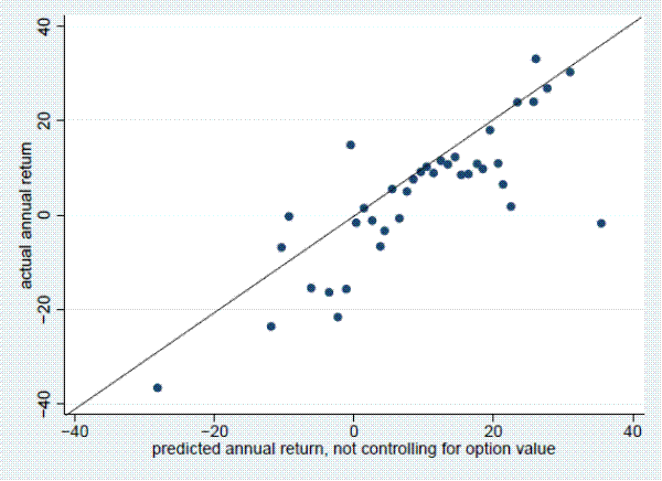
Figures 1 and 2 plot realized returns against returns predicted by the model.¹⁵ Figure 1 corresponds to column I of Table 7, where the structure of the error term is not taken into account, while Figure 2 corresponds to column II, where the option value term is taken into account separately. The differences between the two plots give a graphical representation of the contribution of the option value to improve the fit of the model.

5 The Choice of Opening an Affiliate Abroad: Time-Series Analysis

We plan to exploit the time-series dimension of the data to explore the effect of extensive margin decisions on the returns. First, we compare the stock returns of two groups of domestic firms: firms that stay domestic throughout the sample period, and firms that open affiliates later in the sample period. This will help to address the issue of whether multinational activity drives higher returns, or whether firms that give higher returns self-select into multinational activity. Preliminary results suggest that is multinational activity that drives higher returns.

At a more detailed level, we study the returns' dynamics before and after a firm decides to open an affiliate, and the impact of different location choices for the returns.

Figure 1: Predicted versus realized returns

Figure 2: Predicted versus realized returns, with dummies to control for the option value

6 Conclusions

In this paper we study theoretically and empirically the cross-section of returns of multinational corporations. Stock returns are impacted by firms' diversification of country-level risk, which makes firms safer and decreases returns, and by the sunk costs associated with investing abroad, which make firms more subject to losses, hence riskier, and increases returns. We test the predictions of the model using firm level data on multinational corporations from the US BEA merged with firm level stock return data from CRSP. The empirical results support the model's predictions. MNCs with affiliates in countries where shocks are more highly correlated with US shocks are riskier, and thus require greater equilibrium stock returns. Firms operating in countries where the sunk costs of investing are higher are more likely to bear temporary losses when hit with a negative shock, increasing their risk and implying greater equilibrium stock returns.

References

Atkeson, Andrew, and Tamim Bayoumi. 1993. "Do private capital markets insure regional risk? Evidence from the United States and Europe." Open Economies Review 4:303-324.

Baker, Malcolm, C. Fritz Foley, and Jeffrey Wurgler. 2009. "Multinationals as Arbitrageurs? The Effect of Stock Market Valuations on Foreign Direct Investment." Review of Financial Studies 22 (1): 337-369.

Brainard, S. Lael. 1997. "An Empirical Assessment of the Proximity-Concentration Trade-off between Multinational Sales and Trade." The American Economic Review 87 (4): 520-544.

Branstetter, Lee G., Raymond Fisman, and C. Fritz Foley. 2006. "Do Stronger Intellectual Property Rights Increase International Technology Transfer? Empirical Evidence from U.S. Firm-Level Panel Data."Quarterly Journal of Economics121 (1): 321349.

Carr, David L, James R. Markusen, and Keith E. Maskus. 2001. "Testing the knowledge-capital model of the multinational enterprise." American Economic Review 91 (3): 995-1001.

Cochrane, John H. 2001. Asset Pricing. Princeton, NJ: Princeton University Press.

Crucini, Mario. 1999. "On international and national dimensions of risk sharing." Review of Economics and Statistics8 (1): 73-84.

Das, Sanghamitra, Mark J. Roberts, and James R. Tybout. 2007. "Market Entry Costs, Producer Heterogeneity, and Export Dynamics." Econometrica 75 (3): 837-873.

Denis, David J., Diane K. Denis, and Keven Yost. 2002. "Global Diversification, Industrial Diversification, and Firm Value." The Journal of Finance 57 (5): 1951-1979.

Dixit, Avinash K. 1989. "Entry and Exit Decisions under Uncertainty." Journal of Political Economy97 (3): 620-638.

Dixit, Avinash K., and Robert S. Pindyck. 1994. Investment under Uncertainty. Princeton, NJ:Princeton University Press.

Fama, Eugene F., and Kenneth R. French. 1996. "Multifactor Explanations of Asset Pricing Anomalies." Journal of Finance 51 (1): 55-84.

Fillat, Jose L., and Stefania Garetto. 2012. "Risk, Returns, and Multinational Production." Mimeo, Boston University.

Helpman, Elhanan, Marc J. Melitz, and Stephen R. Yeaple. 2004. "Exports Versus FDI with Heterogeneous Firms." The American Economic Review 94 (1): 300-316.

Jacquillat, Bertrand, and Bruno Solnik. 1978. "Multinationals are poor tools for international diversification." Journal of Portfolio Management4 (2): 812.

Kravis, Irving B., and Robert E. Lipsey. 1982. "The location of overseas production and production for export by U.S. multinational firms." Journal of International Economics 12 (3-4): 201-223.

Markusen, James R., and Keith E. Maskus. 2002. "Discriminating among alternative theories of the multinational enterprise." Review of International Economics10:694-707.

Roberts, Mark J., and James R. Tybout. 1997. "The Decision to Export in Colombia: An Empirical Model of Entry with Sunk Costs." The American Economic Review87 (4): 545-564.

Rowland, Patrick F., and Linda L. Tesar. 2004. "Multinationals and the gains from international diversification." Review of Economic Dynamics7:798-826.

Senchack, Andrew J., and William L. Beedles. 1980. "Is indirect international diversification desirable?" Journal of Portfolio Management6 (2): 49-57.

Sorensen, Bent E., and Oved Yosha. 1998. "International risk sharing and European monetary unification." Journal of International Economics45:211-238.

Tesar, Linda L., and Ingrid Werner. 1998. "The internationalization of securities markets since the 1987 crash." In R. Litan and A. Santomero (eds.), Brookings-Wharton Papers on Financial Services." Washington: The Brookings Institution.

Yeaple, Stephen. 2003. "The Complex Integration Strategies of Multinational Firms and Cross Country Dependencies in the Structure of Foreign Direct Investment." Journal of International Economics 60(2): 293-314.

. 2009."Firm Heterogeneity and the Structure of U.S. Multinational Activity: An Empirical Analysis." Journal of International Economics78 (2): 206-215.

Appendix

We present here the derivation of the results of Section 2. In the continuation region, each one of the three value functions of a firm (, , and ) satisfies:

$\begin{displaymath}\pi(a,Y,X) M\Delta t + E[M\Delta t \cdot V (a,Y',X\vert Y)] - V(a,Y,X) =0.\end{displaymath}$

(A.1)

For $\Delta t \rightarrow 0$ :

$\begin{displaymath}\pi(a,Y,X) M dt + E[d(M \cdot V (a,Y,X))] =0. \end{displaymath}$

(A.2)

The term in the expectation can be written as:

$\displaystyle E[d( M\cdot V)]$	$\textstyle =$	$\displaystyle E[dM \cdot V + M \cdot dV + dM \cdot dV]$
	$\textstyle =$	$\displaystyle M\cdot V \cdot E\left[\frac{dM}{M} + \frac{dV}{V} + \frac{dM}{M} \cdot \frac{dV}{V}\right]$
	$\textstyle =$	$\displaystyle M\cdot V \left[ -r dt + E\left(\frac{dV}{V}\right) + E\left(\frac{dM}{M} \cdot \frac{dV}{V}\right)\right]$
	$\textstyle =$	$\displaystyle Mdt \left[ -r V + E\left(\frac{dV}{dt}\right) + E\left(\frac{dM}{M} \cdot \frac{dV}{dt}\right)\right]$	(A.3)

where the dependence of

has been suppressed to ease the notation. Plugging (A.3) into (A.2):

$\begin{displaymath}\pi - r V + E\left(\frac{dV}{dt}\right) + E\left(\frac{dM}{M} \cdot \frac{dV}{dt}\right) =0. \end{displaymath}$

(A.4)

By applying Ito's Lemma and using the expressions for the Brownian motions ruling the evolution of , we can derive expressions for some of the terms in (A.4):

$\begin{eqnarray*}dV &=& V_Y' dY + \frac{1}{2} {\sigma}^2 Y^2 V_Y$

Using these results and the equation describing the evolution of , we can rewrite (A.4) for the three value functions as:

$\begin{eqnarray*}&& \pi_h dt - r_h V_h dt + \mu_h Y_h {V_h}_Y' dt + \frac{1}{2} ... ...+ \frac{1}{2} \sigma_j^2 Y_j^2 {V_j^o}_Y$

The terms in expectations can be reduced to:

$\begin{eqnarray*}E\left[\left(-r_h dt -\gamma\sigma_h dz_h \right) \cdot \left( ... ...right)\right] &=& -\gamma\rho_j\sigma_h\sigma_j Y {V^o_j}_Y' dt .\end{eqnarray*}$

So we obtain:

$$\displaystyle \pi_h - r_h V_h + (\mu_h -\gamma\sigma_h^2 )Y_h {V_h}_Y' + \frac{1}{2} \sigma_h^2 Y_h^2 {V_h}_Y$	$\textstyle =$	$\displaystyle 0$	(A.5)
$$\displaystyle \pi_j - r_h V_j + (\mu_j -\gamma\rho_j\sigma_h\sigma_j)Y_j {V_j}_Y' + \frac{1}{2} \sigma_j^2 Y_j^2 {V_j}_Y$	$\textstyle =$	$\displaystyle 0$	(A.6)
$$\displaystyle - r_h V^o_j + (\mu_j -\gamma\rho_j\sigma_h\sigma_j)Y_j {V^o_j}_Y' + \frac{1}{2} \sigma_j^2 Y_j^2 {V^o_j}_Y$	$\textstyle =$	$\displaystyle 0.$	(A.7)

Combining the three equations and adding and subtracting the term $\mu_h Y_h {V_h}_Y' + \displaystyle \sum_{j\in {\cal A}} \mu_j Y_j {V_j}_Y' + \displaystyle \sum_{j\not\in {\cal A}} \mu_j Y_j {V^o_j}_Y'$ :

$$\displaystyle \pi_h - r_h V_h -\gamma\sigma_h^2 Y_h {V_h}_Y' + \underbrace{\mu_h Y_h {V_h}_Y' + \frac{1}{2} \sigma_h^2 Y_h^2 {V_h}_Y$
$$\displaystyle \sum_{j\in {\cal A}} \pi_j - r_h V_j -\gamma\rho_j\sigma_h\sigma_j Y_j {V_j}_Y' + \underbrace{\mu_j Y_j {V_j}_Y' + \frac{1}{2} \sigma_j^2 Y_j^2 {V_j}_Y$
$$\displaystyle + \sum_{j\not\in {\cal A}} \left[- r_h V^o_j -\gamma\rho_j\sigma_h\sigma_j)Y_j {V^o_j}_Y' + \underbrace{\mu_j Y_j {V^o_j}_Y' + \frac{1}{2} \sigma_j^2 Y_j^2 {V^o_j}_Y$	$\textstyle =$	$\displaystyle 0.$	(A.8)

Since $E(dV_h)+ \displaystyle \sum_{j\in {\cal A}} E(dV_j) +\displaystyle \sum_{j\not\in {\cal A}} E(dV^o_j) = E(d{\cal V})$ :

$\displaystyle \pi_h + \sum_{j\in {\cal A}}\pi_j + E(d{\cal V})$	$\textstyle =$	$\displaystyle r_h V_h + \gamma\sigma_h^2 Y_h {V_h}_Y' + \sum_{j\in {\cal A}} \left(r_h V_j + \gamma\rho_j\sigma_h\sigma_j Y_j {V_j}_Y'\right) + \sum_{j\not\in {\cal A}} \left(r_h V^o_j + \gamma\rho_j\sigma_h\sigma_j Y_j {V^o_j}_Y'\right)$
$\displaystyle \frac{\pi_h + \displaystyle \sum_{j\in {\cal A}}\pi_j + E(d{\cal V})}{{\cal V}}$	$\textstyle =$	$\displaystyle r_h + \frac{\gamma\sigma_h\left( \sigma_h Y_h {V_h}_Y' + \displaystyle \sum_{j\in {\cal A}} \gamma\rho_j\sigma_j Y_j{V_j}_Y' + \displaystyle \sum_{j\not\in {\cal A}} \gamma\rho_j\sigma_j Y_j{V^o_j}_Y'\right)}{{\cal V}} .$	(A.9)

Footnotes

*The statistical analysis of firm-level data on U.S. multinational companies was conducted at the Bureau of Economic Analysis, U.S. Department of Commerce under arrangements that maintain legal confidentiality requirements. The views expressed are those of the authors and do not reflect official positions of the U.S. Department of Commerce. The authors would like to thank William Zeile and Raymond Mataloni for assistance with the BEA data. Return to Text

** Federal Reserve Bank of Boston, 600 Atlantic Avenue, Boston MA 02210. E-mail: [email protected].org. The views expressed in this paper are those of the authors and do not necessarily reflect those of the Federal Reserve Bank of Boston or Federal Reserve System. Return to Text

* Department of Economics, Boston University, 270 Bay State Road, Boston, MA 02215. E-mail: [email protected]. Return to Text

* Georgetown University, Intercultural Center 515, 37th and O Streets, NW Washington DC, 20057. E-mail: [email protected]. Return to Text

1. Fama and French (1996) provide comprehensive evidence about returns differentials across portfolios formed according to particular characteristics like size and book-to-market. Return to Text

2. Branstetter, Fisman, and Foley (2006) also merge the BEA data on the operations of US multinationals with Compustat data to examine the effect of IPR reforms on technology transfer within multinational corporations. Return to Text

3. While the framework in Fillat and Garetto (2012) distinguishes entry in foreign markets according to whether it happens via export or FDI, in this paper we disregard the decision to export and focus on the choice of becoming a multinational corporation. Return to Text

4. The model does not allow for any possibility of international portfolio diversification, but features perfect home bias in equity portfolios. This assumption is not at odds with the data: Tesar and Werner (1998) provide evidence of an extreme home bias in equity portfolios: about 90% of U.S. equity was invested in the U.S. stock market in the mid-1990s. Atkeson and Bayoumi (1993), Sorensen and Yosha (1998), and Crucini (1999) present evidence supporting the assumption of international market incompleteness. Return to Text

5. The process for the stochastic discount factor

can be derived from agents having CRRA preferences over aggregate consumption

. Return to Text

6. Helpman, Melitz, and Yeaple (2004) model selection into multinational activity as motivated by the interaction of high productivity and fixed costs. The importance of fixed costs for multinational production is documented in the empirical work of Brainard (1997). Roberts and Tybout (1997) and Das, Roberts, and Tybout (2007) show the empirical relevance of sunk costs for entry in foreign markets. Return to Text

7. The model does not accommodate the possibility of bridge multinational production, whereby foreign affiliates of a multinational corporation export to third countries. Return to Text

8. Dixit (1989) provides a seminal treatment of the option value of entry in a model of investment under uncertainty and sunk costs. Return to Text

9. Details of the calculations are relegated to the Appendix. Return to Text

10. We identify firm-level returns with the returns of the firm's common equity. Return to Text

11. We construct this measure using the correlations rather than the covariances of US GDP growth with the host countries. This choice is motivated by the convenience of having a unit-free measure that we can compare with the extreme cases of perfect diversification ( $\rho_{ft} =0$ ) and no diversification ( $\rho_{ft}$ =1). Return to Text

12. Notice that even if the option value component is an omitted variable in regression (13), the results presented in the previous section are not biased. It is reasonable to think that entry costs and GDP growth correlations are not correlated across countries, so the omitted variable is not correlated with the included variable, and the coefficients in Table 2 are not biased. The omitted variable problem will be present instead in our structural specification, as we illustrate in Section 4.3. Return to Text

13. Net income is given by the firm's income from sales and investment minus total costs and expenses, so it is a measure of the firm's affiliate profits in country

. This measure, like flow profits at the affiliate level (which are not available from the BEA data), is not a perfect measure of the value of the firm because it disregards the option value of assets in place. Alternatively, CRSP contains data on profits and market capitalization at the firm level. This measure is also problematic as we only have information on the firm total market capitalization and total profits, not by individual affiliate or country of operation, hence the variation of $\varepsilon_j^f$ across countries only comes from variation in $Y_{j t}$ . To construct $\varepsilon_j^f$ , we also need to take a stand on the status of MNCs that enter or exit countries during the sample period. In our baseline specification, we consider the effect on the returns of those assets that are in place for at least two years of sample period. In the Appendix we report results on the robustness of this assumption. Return to Text

14. The required number of procedures to operate a business in China is 14, versus 6 in the UK and one in Canada. Return to Text

15. To construct the plots, we divided the observations into 50 bins based on their predicted annual returns from regression 15. Then we averaged actual and predicted annual returns within these bins and graphed those averages. Return to Text

^♣ This version is optimized for use by screen readers. Descriptions for all mathematical expressions are provided in LaTex format. A printable pdf version is available. Return to Text

Diversification, Cost Structure, and the Stock Returns of Multinational Corporations*

1 Introduction

2 The Returns of Multinational Corporations

3 Data

Table 1: Summary Statistics

4 The Role of Diversification and Cost Structure: Empirical Results

4.1 Reduced-Form Analysis

Table 2: The relationship between annual returns, GDP growth correlations, and sunk costs.

4.2 Two-Stage Model

Table 3: First stage estimation: selection into FDI.

Table 4: Summary statistics by affiliate presence.

Table 5: Second stage estimation: the relationship between annual returns, GDP growth correlations, and sunk costs, controlling for the option value of entering new countries.

4.3 Structural Analysis

4.3.1 Country-Specific Components of Risk Premium

Table 6: Estimates of and using single host country firms., observations at the firm-year level.

4.3.2 Goodness of Fit

5 The Choice of Opening an Affiliate Abroad: Time-Series Analysis

Figure 1: Predicted versus realized returns

Figure 2: Predicted versus realized returns, with dummies to control for the option value

6 Conclusions

References

Appendix

Footnotes

Diversification, Cost Structure, and the Stock Returns of Multinational Corporations^*

Table 6: Estimates of $\alpha _j$ and $\psi _j$ using single host country firms., observations at the firm-year level.