
Board of Governors of the Federal Reserve System
International Finance Discussion Papers
Number 1019, June 2011 --- Screen Reader
Version*
Limited Market Participation and Asset Prices in the Presence of Earnings Management1
NOTE: International Finance Discussion Papers are preliminary materials circulated to stimulate discussion and critical comment. References in publications to International Finance Discussion Papers (other than an acknowledgment that the writer has had access to unpublished material) should be cleared with the author or authors. Recent IFDPs are available on the Web at http://www.federalreserve.gov/pubs/ifdp/. This paper can be downloaded without charge from the Social Science Research Network electronic library at http://www.ssrn.com/.
Abstract:
We examine the role of earnings management in explaining the properties of asset prices and stock market participation. We demonstrate that investors' uncertainty about the extent of manipulation can cause excess movements in stock price relative to fluctuations in output. When faced with information asymmetry about fundamentals in the presence of earnings management, investors demand a higher equity premium for bearing the additional risk associated with their payoffs. In addition, when investors have heterogeneous beliefs about managerial manipulation, the dispersion in belief endogenously gives rise to limited stock market participation. Our model suggests that the increasing stringency of corporate governance and varying composition of investors may have played a role in the contemporaneous run-up of market participation rates in the recent years.
Keywords: Earnings management, excess volatility, equity premium, limited stock market participation
JEL classification: D82, D83, G12, G14
1 Introduction
Managerial manipulation of financial records can arise in a wide variety of contexts; for example, to window dress financial statements prior to public securities offerings, to increase corporate managers’ compensation, or to avoid violation of lending contracts. Corporate executives have incentives to manipulate earnings, and empirical research on earnings management indicates that they often do.3 The purpose of this paper is to analyze the implication of earnings management for the behavior of asset prices and investment strategies, and thereby shed light on the role of information manipulation in accounting for observed patterns in the stock market.
We construct a simple rational expectations model in which managers have an incentive to portray unjustified success and distort the information content of financial statements, and the market is uncertain about the degree of manipulation. We show that by distinguishing between the cash flows received by equity holders and financial reports released by managers, and by allowing for learning about an unobservable degree of manipulation, it is possible to generate a simple asset pricing model with rational behavior which yields several stylized financial facts. We are primarily interested in the effects that earnings management has on price volatility, equity premium, and stock market participation.
One key feature of our framework is that rational investors are uncertain about the extent of manipulation. Financial statements conflate productivity shocks with earnings management in our model, and even fully rational investors cannot perfectly gauge the true state of the firm in equilibrium. In reality, because the degree of reporting discretion available varies with economic cycles, and managers are not all equally versed in manipulating financial records, shareholders often face bias in the financial results, but cannot determine the extent of the bias. Our model features the substantial discrepancy between market expectations and the firm's underlying financial worth that characterizes many recent corporate scandals.
One implication of our model revolves around the understanding of excess volatility. It has been known for many years that stock prices undergo fluctuations that cannot be justified by subsequent dividends (Shiller (1981) and Leroy and Porter (1981)). In this paper, we show that imperfect information about manipulation generates additional variability in future dividends, and can cause excess movements in stock price relative to fluctuations in dividends. Our model suggests that market uncertainty about underlying states caused by earnings management may be one potential source that amplifies the volatility of relatively stable fundamentals into a fluctuating price series.
In addition, we find that the existence of earnings management can lead to equity premia higher than under truthful reporting. When investors face a significant degree of information asymmetry concerning the extent of manipulation, there is additional uncertainty in firm fundamentals. The perceived opaqueness of financial reporting drives up the equity premium investors demand. Put differently, risk-averse investors are compensated for increased volatility through higher returns on stocks in equilibrium.
The most important application of our model is to examine the relation between the market information about earnings management and the rates of stock market participation. We find that if we allow for beliefs about the degree of manipulation to vary across investors, limited market participation can arise endogenously in equilibrium. When the dispersion of investor beliefs about manipulation is large, investors sufficiently pessimistic about the credibility of financial reporting will consider the market price unjustified by firm value and optimally choose not to invest in stocks in equilibrium.
To study the influence of corporate governance and financial regulations on market participation, we characterize the condition under which the equilibrium rate of market participation increases with the cost of manipulation in our model. The impact of manipulation costs on market participation is determined by how demand for stocks is distributed across investors with heterogeneous beliefs. If the demand is sensitive to investor beliefs of manipulation, a small portion of the most optimistic investors can demand a large volume of stocks, thus driving up the stock price sufficiently high to force out other investors. If investors' demand does not vary much with their beliefs, the equilibrium stock price must adjust to induce a large proportion of investors to hold stocks for the market to clear.
Increasing the cost of falsifying financial records has two effects on the distribution of investor demand. On the one hand, the degree of manipulation is reduced, and thus the demand heterogeneity across investors with differential beliefs becomes smaller. On the other hand, a decreased degree of manipulation brings with it reduced uncertainty of manipulation, causing investor demand to be more sensitive to investor beliefs. When the cost of manipulation is large, the first effect, that is, the effect of reduced importance of investor optimism, dominates, investor demand is less sensitive to investor beliefs when the manipulation cost increases. As a result, the equilibrium participation rate increases to clear the market.
The market participation rate also decreases with the dispersion in investor beliefs about manipulation in our model. Under limited participation, only investors relatively optimistic about reporting credibility invest in stocks. Thus when beliefs about the extent of manipulation become more dispersed, market participants on average have a more favorable view about the accountability of managers' reports and thus the financial worth of the firm. The increased market optimism drives up the equilibrium market price, forcing more investors to withdraw from the market.
Our model builds on previous literature on earnings management. Fischer and Verrecchia (2000) show that more bias in earnings reports reduces the association between share price and reported earnings, and reduces the extent to which price reflects all available information. Guttman et al. (2006) use a signaling model similar to Fischer and Verrecchia (2000) to create an endogenous discontinuity in the distribution of reports. Kwon and Yeo (2009) consider a single-period model where the principal takes into account how compensation affects productive effort and market expectations when designing the optimal contract. In their paper, a rational market can simply recalibrate or discount the reported performance when the manager overstates earnings, and correctly guess the true performance. These papers do not address the issues of price volatility, equity premia, or market participation rates, which are the primary focuses of our paper.
Another branch of literature to which our analysis adheres studies asset pricing under asymmetric information, such as Detemple (1986), Wang (1993), and Cecchetti et al. (2000). In particular, Wang (1993) presents a dynamic asset-pricing model in which investors can be either informed or uninformed: the informed investors know the future dividend growth rate; the uninformed investors do not. He finds that the existence of uninformed investors can lead to risk premia and price volatility much higher than under symmetric and perfect information. Our paper studies the interplay between managers' manipulative incentives and investors' investment strategies, and provides a new explanation for the phenomenon of limited stock market participation.
Our paper is closely related to the literature on limited market participation. Allen and Gale (1994) and Williamson (1994) show that transaction cost and liquidity needs can create limited market participation. Vissing-Jorgensen (1999) and Yaron and Zhang (2000) examine the effect of fixed entry cost on investors' participation decisions. Haliassos and Bertaut (1995) show that risk aversion, heterogeneous beliefs, habit persistence, time-nonseparability, and quantity constraints on borrowing do not account for the observed phenomenon. Among the models that have been proposed to explain why limited market participation may exist, most similar to ours is Cao et al. (2005). They consider uncertainty-averse investors who evaluate an investment strategy according to the expected utility under the worst case probability distribution in a set of prior distributions. They generate limited participation in the presence of model uncertainty and heterogeneous uncertainty-averse investors. This paper can be viewed as complementary to theirs in that our results indicate that limited participation can arise endogenously in the presence of earnings management without behavioral utility specifications. In addition, our model yields implications of how corporate governance policies and financial regulations influence market participation rates.
Existing studies have analyzed earnings management behavior and stylized financial facts in isolation, and there have not been many theoretical studies that investigate the systematic link between manipulation and financial anomalies. Sun (2010) represents an exception and shows that embedding a contracting problem into an otherwise standard asset-pricing model can account for a number of observed features of return volatility. In this paper, we instead study capital market considerations in managerial reporting decisions and incorporate heterogeneous investor beliefs of earnings manipulation. Furthermore, we examine the implications of information manipulation for the equilibrium equity premium and market participation rate, which are not addressed in Sun (2010).
We organize this paper as follows. Section 2 lays out the formal model, and we consider a simple environment in which the manager reports truthfully and investors are homogeneous and perfectly informed. This provides a benchmark case for our analysis. The equilibrium of the full model is characterized in Section 3. In Section 4, we investigate how investors' uncertainty about managerial manipulation affects price volatility and equity premium. In Section 5, we extend the model to allow for heterogeneous investor beliefs about the extent of manipulation. Section 6 analyzes the equilibrium market participation rate. Section 7 concludes.
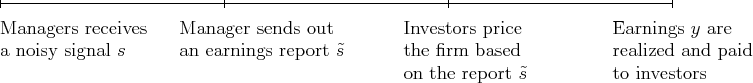
Figure 1: Model Timeline
2 Model
We consider a simple one-period economy with a representative firm.
True earnings ![]() are drawn from a normal distribution with
mean
are drawn from a normal distribution with
mean ![]() and variance
and variance ![]() . The
time line of Figure 1 chronicles the sequence of
events in the model. Before the stock is traded in the market, the
manager of the firm receives a private signal of the future
realization of earnings, that is,
. The
time line of Figure 1 chronicles the sequence of
events in the model. Before the stock is traded in the market, the
manager of the firm receives a private signal of the future
realization of earnings, that is,
![]() , where
, where ![]() is
the productivity shock to the firm value and follows a normal
distribution:
is
the productivity shock to the firm value and follows a normal
distribution:
![]() . The
manager is mandated to publish a report of his private signal,
denoted by
. The
manager is mandated to publish a report of his private signal,
denoted by ![]() , which investors use to make their
investment strategies. At the end of the period, final payoffs are
established and earnings (
, which investors use to make their
investment strategies. At the end of the period, final payoffs are
established and earnings (![]() ) are distributed to
investors as dividends.
) are distributed to
investors as dividends.
If the manager produces an inaccurate report, the manager incurs
a personal cost, denoted by ![]() , where
, where
![]() . The discrepancy between the
original signal and the financial report,
. The discrepancy between the
original signal and the financial report, ![]() , is
interpreted as the amount of manipulation undertaken by the
manager.
, is
interpreted as the amount of manipulation undertaken by the
manager. ![]() is a quadratic function of
is a quadratic function of
![]() :
:
![]() , where
, where ![]() is a known positive parameter, and
is a known positive parameter, and ![]() is a
parameter unknown to investors. The cost of manipulation thus
involves a deterministic component (
is a
parameter unknown to investors. The cost of manipulation thus
involves a deterministic component (![]() ) and a
stochastic component (
) and a
stochastic component (![]() ).
). ![]() can be
interpreted as a policy parameter that is influenced by governance
policies and regulatory stringency, and the value of
can be
interpreted as a policy parameter that is influenced by governance
policies and regulatory stringency, and the value of ![]() is public information. We also assume that the marginal
cost of inflating reports increases with the deviation from the
original signal, which is determined by
is public information. We also assume that the marginal
cost of inflating reports increases with the deviation from the
original signal, which is determined by ![]() .
.
We assume that ![]() is a random draw from a
normal distribution:
is a random draw from a
normal distribution:
![]() . Investors know
the distribution of
. Investors know
the distribution of ![]() , but the true value of
, but the true value of
![]() remains the manager's private
information.4 The unobserved heterogeneity of
remains the manager's private
information.4 The unobserved heterogeneity of
![]() is intended to capture the notion that
manipulating financial records often involves personal costs or
benefits the market does not precisely know. For example, investors
may not have perfect information about managers' time horizon,
personal stigma, the degree of risk-aversion, the costs involved in
bribing auditors not to report a discrepancy in financial
statements, or the amount of resources and effort required to
modify financial records. Note that
is intended to capture the notion that
manipulating financial records often involves personal costs or
benefits the market does not precisely know. For example, investors
may not have perfect information about managers' time horizon,
personal stigma, the degree of risk-aversion, the costs involved in
bribing auditors not to report a discrepancy in financial
statements, or the amount of resources and effort required to
modify financial records. Note that ![]() can be
positive or negative, reflecting the fact that some managers have
preferences towards positive manipulation and some managers have
preferences towards negative manipulation. In particular, a manager
with a negative
can be
positive or negative, reflecting the fact that some managers have
preferences towards positive manipulation and some managers have
preferences towards negative manipulation. In particular, a manager
with a negative ![]() prefers a larger ("more
positive") manipulation than a manager with a positive
prefers a larger ("more
positive") manipulation than a manager with a positive ![]() . In reality, we observe earnings manipulation in both
directions. The financial report (
. In reality, we observe earnings manipulation in both
directions. The financial report (![]() )
thereby conflates the exogenous shock to the firm value and the
amount of manipulation (influenced by
)
thereby conflates the exogenous shock to the firm value and the
amount of manipulation (influenced by ![]() ). This
assumption of unobserved manipulation cost is motivated by
the substantial discrepancy between investors' expectations and the
underlying financial worth of the firm highlighted by many recent
financial scandals.
). This
assumption of unobserved manipulation cost is motivated by
the substantial discrepancy between investors' expectations and the
underlying financial worth of the firm highlighted by many recent
financial scandals.
Let ![]() denote the price of the stock
given the report
denote the price of the stock
given the report ![]() . The manager's utility is
given by
. The manager's utility is
given by
The first term reflects the manager's desire to maximize the share price of the firm. The second term is the manager's cost of manipulating the report. Typically, managers prefer higher stock prices, as their managerial compensation is often directly or indirectly tied to the firm's stock market performance. Another interpretation of this term is that managers want to boost share price before the firm's initial public offerings.
The objective of the manager in this environment is to maximize
his utility by choosing a reporting strategy represented by
![]() , subject to the market reaction.
, subject to the market reaction.
| (1) |
The quantity of stock is normalized to one perfectly divisible
share. There is a risk-free asset available to investors at no
cost. The risk-free asset is sold at a constant price ![]() and yields a constant return
and yields a constant return ![]() .
All investors in the economy have preferences exhibiting constant
absolute risk aversion (CARA) and have initial wealth
.
All investors in the economy have preferences exhibiting constant
absolute risk aversion (CARA) and have initial wealth ![]() to invest in the firm's stock and one risk-free asset. The
investors' utility is defined as
to invest in the firm's stock and one risk-free asset. The
investors' utility is defined as
where ![]() is investors' terminal wealth and
is investors' terminal wealth and
![]() is investors' risk-aversion
coefficient. Investors' wealth constraints are
is investors' risk-aversion
coefficient. Investors' wealth constraints are
and
where ![]() and
and ![]() are the investors'
demand for the firm's asset and the risk-free asset respectively.
In the following, we permit the case where
are the investors'
demand for the firm's asset and the risk-free asset respectively.
In the following, we permit the case where ![]() , for
ease of exposition. Under the assumption of normality5 and CARA
utility, the investors' utility maximization problem becomes:
, for
ease of exposition. Under the assumption of normality5 and CARA
utility, the investors' utility maximization problem becomes:
| (2) |
where
![]() is the expected value
given the report
is the expected value
given the report ![]() and
and
![]() is the variance given
is the variance given
![]() . This indicates a linear tradeoff
between the mean and variance of terminal wealth. With CARA utility
functions, investors' demand for stocks is independent of their
initial wealth. This implies that the equilibrium price and
participation strategies are independent of the level of aggregate
wealth and the wealth distribution of investors.
. This indicates a linear tradeoff
between the mean and variance of terminal wealth. With CARA utility
functions, investors' demand for stocks is independent of their
initial wealth. This implies that the equilibrium price and
participation strategies are independent of the level of aggregate
wealth and the wealth distribution of investors.
A Perfect Bayesian Equilibrium is defined as a reporting
strategy ![]() for the manager, joint with a pricing
function
for the manager, joint with a pricing
function ![]() for investors, such that:
for investors, such that:
- Given the manager's reporting strategy
 and
the pricing rule
and
the pricing rule  , investors maximize their
expected utility. Beliefs are consistent with Bayes' rule.
, investors maximize their
expected utility. Beliefs are consistent with Bayes' rule. - Given the pricing function,
 maximizes the
utility of the manager.
maximizes the
utility of the manager. - Market clearing requires that the stock voluntarily held by
investors (denoted by
 ) be equal to the total
quantity of the stock.
) be equal to the total
quantity of the stock.
Before we solve the full model, let us first consider the
special case in which there is no possibility of manipulation, that
is,
![]() . The equilibrium
price under truthful reporting provides a benchmark for the value
of the stock, and will serve as a basis for comparison with the
stock price dynamics in the presence of manipulation that will be
analyzed in Section 3.
. The equilibrium
price under truthful reporting provides a benchmark for the value
of the stock, and will serve as a basis for comparison with the
stock price dynamics in the presence of manipulation that will be
analyzed in Section 3.
Under truthful reporting, investors maximize their expected
utility by choosing how much to invest in the firm's stock and how
much to park in a risk-free asset. Given investors' portfolio
choice, market clearing is then imposed to determine the
equilibrium stock price. Let
![]() denote the equilibrium
stock price given the report (
denote the equilibrium
stock price given the report (![]() ) in the
absence of manipulation. We have the following result.
) in the
absence of manipulation. We have the following result.
Proposition 1 Under truthful reporting, the firm's
stock price given the report, ![]() , can be
expressed as
, can be
expressed as
| (3) |
Proof: See Appendix A.
The equilibrium stock price is the risk adjusted present value
of future dividends discounted at the risk-free rate. Here
![]() is the expected output. The term
is the expected output. The term
![]() represents the
discount on the stock price to compensate for the risk in the
future dividends, which is proportional to investors' risk-aversion
coefficient and the variance of productivity shock. As
represents the
discount on the stock price to compensate for the risk in the
future dividends, which is proportional to investors' risk-aversion
coefficient and the variance of productivity shock. As
![]() increases, the price of the
stock has to adjust to generate a higher expected return in order
to induce investors to hold the stock.
increases, the price of the
stock has to adjust to generate a higher expected return in order
to induce investors to hold the stock.
Given the equilibrium price of the stock, the return on the
firm's stock, denoted by ![]() , is the true earnings
(
, is the true earnings
(![]() ) divided by the market price (
) divided by the market price (![]() ). The expected excess return on equity under
truthful reporting is
). The expected excess return on equity under
truthful reporting is
![]() .
. ![]() only depends on
only depends on
![]() , which characterizes the
risk associated with future dividends of the stock. Below we show
that the price volatility and excess return on the firm's stock
increase with fundamental uncertainty
, which characterizes the
risk associated with future dividends of the stock. Below we show
that the price volatility and excess return on the firm's stock
increase with fundamental uncertainty
![]() .
.
Lemma 1 Stock price volatility (![]() ) and
equity premium (
) and
equity premium (![]() ) are increasing in
) are increasing in
![]() .
.
Proof: See Appendix A.
3 Stock Price with Manipulation
When manipulation is possible, in our model truthful reporting
(that is,
![]() ) does not in general
constitute an equilibrium, because there is an incentive to alter
the reporting strategy ex-post. If the market believed in the face
value of the reports, the manager would have an incentive to
overstate the report for an inflated share price.
) does not in general
constitute an equilibrium, because there is an incentive to alter
the reporting strategy ex-post. If the market believed in the face
value of the reports, the manager would have an incentive to
overstate the report for an inflated share price.
In the presence of manipulation opportunities, the equilibrium
stock price and excess return on the stock depend on the
information structure of the economy. When investors have perfect
information about manipulation costs (![]() as well as
as well as
![]() ), they correctly subtract out the
manipulation component from the report when they value the firm.
This type of signal jamming equilibrium is inefficient, because the
manager takes a costly action to mislead but ends up misleading no
one in the equilibrium. The cost associated with manipulation is
borne by the manager; since no market player benefits from
manipulating reports, it imposes a deadweight loss on the economy.
This signal jamming equilibrium is standard in the
literature6, and in Appendix B we show that the
behavior of the equilibrium stock price is identical to that in the
benchmark case.
), they correctly subtract out the
manipulation component from the report when they value the firm.
This type of signal jamming equilibrium is inefficient, because the
manager takes a costly action to mislead but ends up misleading no
one in the equilibrium. The cost associated with manipulation is
borne by the manager; since no market player benefits from
manipulating reports, it imposes a deadweight loss on the economy.
This signal jamming equilibrium is standard in the
literature6, and in Appendix B we show that the
behavior of the equilibrium stock price is identical to that in the
benchmark case.
In the remaining part of this section we solve for the
equilibrium of the full model specified in Section 2, in which
investors know the probability distribution of ![]() but are unable to observe the actual value of
but are unable to observe the actual value of ![]() .
In reality, manipulation may carry higher regulatory costs for
firms with stringent internal control systems over financial
reporting, and may involve higher psychological costs for some
managers than others. In addition, managers are not equally versed
in inflating reports and are thus subject to differential learning
costs. Investors do not know how costly it is for the manager of
one particular firm to manipulate financial results.
.
In reality, manipulation may carry higher regulatory costs for
firms with stringent internal control systems over financial
reporting, and may involve higher psychological costs for some
managers than others. In addition, managers are not equally versed
in inflating reports and are thus subject to differential learning
costs. Investors do not know how costly it is for the manager of
one particular firm to manipulate financial results.
The procedure we follow to obtain an equilibrium of the economy is similar to that of Grossman (1976). We first conjecture an equilibrium pricing function and an equilibrium reporting function. Based on the assumed pricing function, we solve the manager's optimization problem, and based on the assumed reporting function, we solve the investors' investment problem. The market clearing condition is then imposed to verify the conjectured pricing and reporting functions.
3.1 Manager's Reporting Strategy
Since we expect the equilibrium stock price to resemble the
functional form of the price in the benchmark case, we first guess
that the price of the firm is a linear function of the report:
![]() . With the
conjectured price function, the first-order condition for the
manager's problem (1)
yields
. With the
conjectured price function, the first-order condition for the
manager's problem (1)
yields
| (4) |
and therefore
| (5) |
for all ![]() . Note that even when
. Note that even when ![]() is
equal to zero, the amount of manipulation can be positive since the
manipulation can change the stock price. The extent of manipulation
is increasing in the sensitivity of stock price to managerial
reports (
is
equal to zero, the amount of manipulation can be positive since the
manipulation can change the stock price. The extent of manipulation
is increasing in the sensitivity of stock price to managerial
reports (![]() ) and decreasing in the manipulation cost
(
) and decreasing in the manipulation cost
(![]() and
and ![]() ). The manager
faces a trade-off in reporting: on the one hand, he wants to
manipulate the report to bump up the stock price; on the other
hand, he does not want to inflate the performance too much because
of the increasing marginal cost of manipulation. Since the marginal
benefit of manipulating reports is constant across different levels
of earnings, and the marginal cost is linear in the amount of
manipulation, this trade-off determines an optimal level of
manipulation (
). The manager
faces a trade-off in reporting: on the one hand, he wants to
manipulate the report to bump up the stock price; on the other
hand, he does not want to inflate the performance too much because
of the increasing marginal cost of manipulation. Since the marginal
benefit of manipulating reports is constant across different levels
of earnings, and the marginal cost is linear in the amount of
manipulation, this trade-off determines an optimal level of
manipulation (![]() ) that is independent of the original
signal
) that is independent of the original
signal ![]() the manager privately observes. Because
the manager privately observes. Because
![]() is not precisely known to investors, the
amount of manipulation remains private information of the manager.
is not precisely known to investors, the
amount of manipulation remains private information of the manager.
Note that now the amount of manipulation, ![]() ,
can be expressed as a function of the random variable
,
can be expressed as a function of the random variable ![]() . Therefore,
. Therefore, ![]() itself is a random variable.
With an abuse of notation, from here on, let us denote
itself is a random variable.
With an abuse of notation, from here on, let us denote ![]() as this random variable, with relationship (5) in mind. Note
that
as this random variable, with relationship (5) in mind. Note
that ![]() follows a normal distribution with
mean
follows a normal distribution with
mean
| (6) |
and variance

Note that ![]() still contains an unknown
still contains an unknown
![]() at this point.
at this point.
3.2 Investors' Investment Decision
We will check whether the equilibrium value of ![]() is in fact linear in
is in fact linear in ![]() , as we conjectured.
Given the manager's report, investors form their expectation of the
future wealth as follows:
, as we conjectured.
Given the manager's report, investors form their expectation of the
future wealth as follows:
![\begin{eqnarray*} E[W\vert\tilde s] &=& E[y\vert \tilde s] q + q_f \ &=& E[\tilde s- m - \epsilon]q+(W_0-p q)/p_f \ &=& (\tilde s-\mu_m)q+(W_0-p q)/p_f,\ Var[W\vert\tilde s] &=& q^2 Var[y\vert \tilde s] = q^2 (\sigma_m^2+ \sigma^2_\epsilon). \end{eqnarray*}](img108.gif)
Substituting these into investors' objective function (2), the investors' problem is given by7
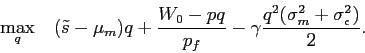
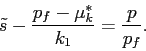
The optimization problem of investors can be characterized by the following first-order condition:
Solving for the optimal share of the stock investors are willing to hold, we arrive at the following expression.
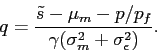 |
(7) |
Investors' demand for the stock increases with the reported
profitability adjusted by the average amount of manipulation (
![]() ). It is low when the relative
price of the stock (
). It is low when the relative
price of the stock (![]() ), investors' risk
aversion (
), investors' risk
aversion (![]() ), productivity uncertainty (
), productivity uncertainty (
![]() ), and manipulation
uncertainty (
), and manipulation
uncertainty (![]() ) are high.
) are high.
3.3 Equilibrium Stock Price
Under the conjectured forms of the price function and reporting function, the demand for the stock by investors is given by (7). When the market clears, it must be equal to the quantity of stock available, which is normalized to 1. Thus,
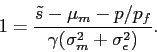
The equilibrium stock price is
Therefore, the price is in fact linear in ![]() ,
and matching the coefficients with the conjecture
,
and matching the coefficients with the conjecture
![]() , noting
that
, noting
that ![]() is given by (6), yields the
solutions
is given by (6), yields the
solutions
and
where ![]() is now given by
is now given by
so that
We summarize the results below.
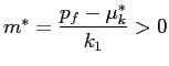
Proposition 2 Under earnings management, the equilibrium price of the stock can be expressed as
| (8) |
where
![]() and
and
![]() . The optimal
reporting strategy of the manager is
. The optimal
reporting strategy of the manager is
| (9) |
Given the stock price ![]() , the demand for the
stock by investors,
, the demand for the
stock by investors, ![]() , is given by
, is given by
 |
(10) |
Similar to the benchmark case without manipulation, the
equilibrium stock price is the risk adjusted present value of
expected future dividends discounted at the risk-free rate.
Investors subtract the expected amount of manipulation (![]() ) from the manager's report to value the firm. The last
term in (8),
) from the manager's report to value the firm. The last
term in (8),
![]() ,
represents the discount on the price of the stock to compensate for
the risk in future dividends.
,
represents the discount on the price of the stock to compensate for
the risk in future dividends.
Based on the distribution of manipulation costs, investors are
able to infer the average amount of manipulation (![]() ). They discount the value of the firm accordingly to
adjust for the bias in the report. Since investors do not have
perfect knowledge about the cost and therefore the degree of
manipulation, they have to treat the firm as if the manager is
subject to the average
). They discount the value of the firm accordingly to
adjust for the bias in the report. Since investors do not have
perfect knowledge about the cost and therefore the degree of
manipulation, they have to treat the firm as if the manager is
subject to the average ![]() . Investors underestimate
the overstatement and over-price the firm if the manager draws a
below-average manipulation cost
. Investors underestimate
the overstatement and over-price the firm if the manager draws a
below-average manipulation cost ![]() , and
investors undervalue the firm otherwise.
, and
investors undervalue the firm otherwise.
Our model can be extended to incorporate heterogeneous firms
that differ in their underlying productivity (![]() )
as well as their manipulation cost (
)
as well as their manipulation cost (![]() ), both of
which are stochastic and unobservable to investors. One key feature
that arises from such an information structure is that predicting
individual future output is harder than predicting the aggregate
level of future output. Managerial manipulation obscures individual
firms' financial condition, and equilibrium stock prices are not
fully-revealing in this case.
), both of
which are stochastic and unobservable to investors. One key feature
that arises from such an information structure is that predicting
individual future output is harder than predicting the aggregate
level of future output. Managerial manipulation obscures individual
firms' financial condition, and equilibrium stock prices are not
fully-revealing in this case.
4 Price Volatility and Equity Premia
We next examine how earnings management affects price volatility
and equity premia. In the current model, the parameter ![]() characterizes investors' uncertainty about the
degree of manipulation. Most of the comparative static analysis in
this section is concerned with the effect of changing
characterizes investors' uncertainty about the
degree of manipulation. Most of the comparative static analysis in
this section is concerned with the effect of changing ![]() . The case
. The case ![]() corresponds to the case of perfect information in which investors
see through manipulation and correctly gauge the true state of the
firm. As discussed in Appendix B, in such a signal jamming
equilibrium, manipulation does not have any systematic impact on
the efficiency of the equilibrium stock price. Comparing the
results for
corresponds to the case of perfect information in which investors
see through manipulation and correctly gauge the true state of the
firm. As discussed in Appendix B, in such a signal jamming
equilibrium, manipulation does not have any systematic impact on
the efficiency of the equilibrium stock price. Comparing the
results for ![]() and
and
![]() illustrates the effect of
information asymmetry caused by manipulation.
illustrates the effect of
information asymmetry caused by manipulation.
4.1 Price Volatility
Let us consider how earnings management affects the volatility of stock prices. As stated in Proposition 2, the equilibrium price of the stock under earnings management is
The term
![]() represents the discount on
the price to compensate for the additional risk (caused by the
possibility of manipulation) in future dividends, and the
equilibrium stock price monotonically decreases with
represents the discount on
the price to compensate for the additional risk (caused by the
possibility of manipulation) in future dividends, and the
equilibrium stock price monotonically decreases with ![]() , and therefore in
, and therefore in ![]() .
Because of the additional uncertainty about the firm's cost
involved in manipulating reports, investors cannot perfectly infer
the true value of the firm. The additional uncertainty about future
asset payoffs causes excess movements in stock prices relative to
fundamentals.
.
Because of the additional uncertainty about the firm's cost
involved in manipulating reports, investors cannot perfectly infer
the true value of the firm. The additional uncertainty about future
asset payoffs causes excess movements in stock prices relative to
fundamentals.
Proposition 3 The unconditional variance of the stock price is higher
under earnings management than under truthful reporting and is
increasing in ![]() , i.e.,
, i.e., ![]() , and
, and
![]() .
.
Proof: See Appendix C.
The literature acknowledges that stock price volatility systematically exceeds levels justified by fundamentals. The papers by Shiller (1981) and Leroy and Porter (1981) were the first to show that the volatility of stock prices grossly exceeds the volatility of ex-post dividends. In our model, market uncertainty about the degree of manipulation can cause stock prices to move more than is warranted by changes in fundamentals. Although actual dividends do not vary much, information asymmetry concerning the firm' underlying state can cause additional movements in stock prices.
One hurdle to our intuition may arise in a long-term investment horizon -- can there be uncertainty about firms' financial reporting credibility, period after period, that does not disappear so quickly that undermines our mechanism? Companies constantly face new risks and business opportunities that are associated with varying costs involved in manipulating financial records and thus call for continued reevaluation of firms. As illustrated by many cases of real-world corporate scandals, investors find it difficult to determine how much the financial results have been inflated.
4.2 Equity Premium
The equity premium on the stock is given by
![]() , where we
only consider the situation when
, where we
only consider the situation when ![]() . As investors
cannot perfectly gauge the true state of the firm, they demand a
higher premium for bearing additional risk associated with their
asset payoffs.
. As investors
cannot perfectly gauge the true state of the firm, they demand a
higher premium for bearing additional risk associated with their
asset payoffs.
Proposition 4 The equity premium on a firm's stock
(![]() ) is higher under earnings management than
under truthful reporting and is increasing in manipulation
uncertainty (
) is higher under earnings management than
under truthful reporting and is increasing in manipulation
uncertainty (![]() ).
).
Proof: See Appendix C.
The equity premium in the current model only depends on the
fundamental risk perceived by investors. When manipulation
uncertainty (![]() ) increases, this increases
investors' uncertainty about future dividends, and therefore also
increases the risk of investing in the stock. In equilibrium, a
higher premium on the stock is required to induce investors to hold
the stock. Put differently, risk-averse investors are compensated
for increased volatility through higher expected return on
stocks.
) increases, this increases
investors' uncertainty about future dividends, and therefore also
increases the risk of investing in the stock. In equilibrium, a
higher premium on the stock is required to induce investors to hold
the stock. Put differently, risk-averse investors are compensated
for increased volatility through higher expected return on
stocks.
It is argued that stock returns are too high relative to the return on risk-less assets to be explicable without assuming a very high level of risk aversion on the part of the representative agent. The apparent discrepancy between the low volatility of dividends and the high volatility of stock prices is a fundamental element of the equity premium puzzle: unless we understand why equities are risky we cannot understand why investors demand a significant equity premium. Because earnings management obscures corporate performance and magnifies market volatility, we show that the premium on equity increases to justify this extra risk component.
5 Portfolio Choices and Market Participation
In this section, we study the implication of earnings management
for stock market participation. So far, we have conducted the
analysis in a representative-agent framework. In accordance with
our earlier interpretation of manipulation, one can easily imagine
an economy characterized by heterogeneous investor beliefs about
the extent of earnings manipulation. Diverse perceptions of
manipulation can arise for a number of reasons. For example,
investors with access to different (non-public) information about
the firm's internal control system over financial reporting have
different perceptions about ![]() . Investors may
also arrive at different subjective assessments even when they have
the same substantive information. In addition, differences in
investors' ability to see through (part of) the manipulation can
contribute to the heterogeneity in the perceived degree of
manipulation. The equilibrium price in this environment is obtained
through market aggregation of diverse investor assessments.
. Investors may
also arrive at different subjective assessments even when they have
the same substantive information. In addition, differences in
investors' ability to see through (part of) the manipulation can
contribute to the heterogeneity in the perceived degree of
manipulation. The equilibrium price in this environment is obtained
through market aggregation of diverse investor assessments.
Let the expected value of ![]() (i.e.,
(i.e.,
![]() ) be dispersed across investors instead
of a constant and common parameter. We assume that
) be dispersed across investors instead
of a constant and common parameter. We assume that ![]() is uniformly distributed among investors on the
interval
is uniformly distributed among investors on the
interval
with density ![]() , where
, where
![]() and
and ![]() measures the dispersion of the expected amount of
manipulation among investors. When
measures the dispersion of the expected amount of
manipulation among investors. When ![]() , the
model is reduced to our representative-agent model in Section 3. Recall that
investors "adjust" the report by the expected value of
manipulation and react to
, the
model is reduced to our representative-agent model in Section 3. Recall that
investors "adjust" the report by the expected value of
manipulation and react to
![]() , where
, where
![]() . An investor who
believes that
. An investor who
believes that ![]() is high expects a small (or
negative) amount of average manipulation
is high expects a small (or
negative) amount of average manipulation ![]() , and
perceives a high actual performance for a given
, and
perceives a high actual performance for a given ![]() . An investor who believes
. An investor who believes ![]() is low
thinks there is a large positive manipulation, and undervalues the
firm compared to the report. Investors with
is low
thinks there is a large positive manipulation, and undervalues the
firm compared to the report. Investors with
![]() are referred to as
"optimistic investors"; investors with
are referred to as
"optimistic investors"; investors with
![]() are referred to as
"pessimistic investors" hereafter.
are referred to as
"pessimistic investors" hereafter.
Our model follows the key insight of Harrison and Kreps (1978) and Scheinkman and Xiong (2003) that when investors agree to disagree, asset prices may differ from fundamental values. Similar to both papers, we assume that investors do not turn to public information, such as stock prices, to discover what their fellow investors know and how they react to information.
In this section, we first revisit investors' optimal portfolio-holding problem, and derive the condition under which all investors participate in the stock market. Next we turn to analyze the properties of the equilibrium stock price. Finally, we solve for the equilibrium participation rate. We show that when investors have heterogeneous beliefs about the extent of manipulation, there is limited market participation in equilibrium. In addition, the equilibrium participation rate varies with the manipulation cost and belief dispersion.
5.1 Full Participation
For an investor with ![]() , the investor's optimal
holding in the stock is given by Equation (10) restated
below:
, the investor's optimal
holding in the stock is given by Equation (10) restated
below:
 |
(11) |
Investors' demand for the stock is strong if the manager's
report is high and if the investor's risk aversion ![]() , the expected amount of manipulation
, the expected amount of manipulation
![]() , the intrinsic uncertainty
about fundamentals
, the intrinsic uncertainty
about fundamentals
![]() , and the uncertainty
about manipulation
, and the uncertainty
about manipulation ![]() are low.
are low.
If investors have homogeneous views of ![]() , the
equilibrium price
, the
equilibrium price ![]() is set such that the
representative investor holds one share and the market clears. Full
market participation prevails in equilibrium by construction.
is set such that the
representative investor holds one share and the market clears. Full
market participation prevails in equilibrium by construction.
Now let us consider an environment in which investors are
uncertain about the average degree of manipulation and have varying
beliefs about ![]() . The higher the overstatement
. The higher the overstatement
![]() investors perceive, the lower
the estimated firm value, and the lower demand for the stock. We
assume that a short sale is not permitted. In equilibrium all
investors participate in the market if the most pessimistic
investor (i.e., the investor with the lowest
investors perceive, the lower
the estimated firm value, and the lower demand for the stock. We
assume that a short sale is not permitted. In equilibrium all
investors participate in the market if the most pessimistic
investor (i.e., the investor with the lowest ![]() :
:
![]() ) holds the stock.
This implies
) holds the stock.
This implies
 |
(12) |
Using the market clearing condition,
![\begin{displaymath} 1=\int^{\bar\mu_k+\theta}_{\bar\mu_k-\theta} \displaystyle \frac{1}{2\theta} \left[\frac{\tilde s-(p_f-\mu_k)/k_1-p/p_f}{\gamma(\sigma_m^2+ \sigma^2_\epsilon)} \right] d\mu_k, \end{displaymath}](img193.gif)
we solve for ![]() as follows.
as follows.
Under full market participation, the market price behaves as if
all investors have the average perception of manipulation
![]() . We assume that market clearing
prices are positive under relevant parameterization. Because the
expression of the equilibrium stock price is identical to that of
the representative investors economy, the comparative static
results of price volatility and equity premia around
. We assume that market clearing
prices are positive under relevant parameterization. Because the
expression of the equilibrium stock price is identical to that of
the representative investors economy, the comparative static
results of price volatility and equity premia around ![]() derived in Section 4 remain valid
when all investors with heterogeneous beliefs participate in the
stock market.
derived in Section 4 remain valid
when all investors with heterogeneous beliefs participate in the
stock market.
The dispersion in investors' perceptions has no impact on prices
in this case. An increased dispersion of investor beliefs
(![]() ) does not change the proportion of
optimistic investors and pessimistic investors participating in the
market under full participation. Due to the symmetry in the
distribution of investors' perceived overstatement (and therefore
firm value), the average manipulation perceived by investors
determines the equilibrium stock price. The investors who are more
optimistic about the reliability of reporting and thus the value of
the firm will hold more stock, while investors whose estimated
overstatement is relatively higher will hold less.
) does not change the proportion of
optimistic investors and pessimistic investors participating in the
market under full participation. Due to the symmetry in the
distribution of investors' perceived overstatement (and therefore
firm value), the average manipulation perceived by investors
determines the equilibrium stock price. The investors who are more
optimistic about the reliability of reporting and thus the value of
the firm will hold more stock, while investors whose estimated
overstatement is relatively higher will hold less.
Combining this with Equation (12), we have that in the equilibrium all investors participate in the market if
| (13) |
This full participation condition indicates that whether the most
pessimistic investor participates in the stock market depends on
the dispersion in investors' perceptions of manipulation. When ![]() is sufficiently small, the
discrepancy in the perceived degree of manipulation among investors
is small enough such that all investors are willing to hold a
positive share of the stock under the equilibrium market price.
When investor beliefs about manipulation are distinguishable enough
that condition (13)
is not satisfied, some investors will consider the equilibrium
price too high for their estimated firm worth and optimally
withdraw from the stock market.
is sufficiently small, the
discrepancy in the perceived degree of manipulation among investors
is small enough such that all investors are willing to hold a
positive share of the stock under the equilibrium market price.
When investor beliefs about manipulation are distinguishable enough
that condition (13)
is not satisfied, some investors will consider the equilibrium
price too high for their estimated firm worth and optimally
withdraw from the stock market.
5.2 Limited Participation
When investors have distinct views about the extent of
overstatement, the investors sufficiently pessimistic about the
credibility of financial reporting will consider the market price
unjustified by the underlying value of the firm. If short selling
is not permitted, they withdraw from the stock market. Let
![]() denote the lowest level of belief
about
denote the lowest level of belief
about ![]() at which investors hold the stock. The
investor with
at which investors hold the stock. The
investor with ![]() is referred to as the "marginal
investor" hereafter. Then we have
is referred to as the "marginal
investor" hereafter. Then we have
 |
(14) |
Using the market clearing condition,
![\begin{displaymath} 1=\int^{\bar\mu_k+\theta}_{\mu^*_k} \displaystyle \frac{1}{2\theta} \left[\frac{\tilde s-(p_f-\mu_k)/k_1-p/p_f}{\gamma(\sigma_m^2+ \sigma^2_\epsilon)} \right] d\mu_k, \end{displaymath}](img205.gif)
and combining this with Equation (14), we arrive at
the following expression that determines ![]() .
.
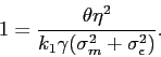
![\begin{displaymath} 1= \frac{[(\bar\mu_k+\theta)-\mu^*_k]^2}{4 k_1 \theta \gamma(\sigma_m^2+ \sigma^2_\epsilon)}. \end{displaymath}](img207.gif) |
(15) |
5.3 Equilibrium Stock Price Under Limited Participation
5.3.1 Effects of Corporate Governance
In our model, ![]() is a policy parameter influenced by
public governance policies and accounting standards. Let us first
consider how
is a policy parameter influenced by
public governance policies and accounting standards. Let us first
consider how ![]() influences the equilibrium stock
price by influencing investor demand for the stock. The direct
effect of increasing
influences the equilibrium stock
price by influencing investor demand for the stock. The direct
effect of increasing ![]() is to affect stock prices
through the extensive margin (that is, the marginal investor). To
see this clearly, we rewrite Equation (14) as follows.
is to affect stock prices
through the extensive margin (that is, the marginal investor). To
see this clearly, we rewrite Equation (14) as follows.
 |
(16) |
The right-hand side is the relative price of the stock and can be
considered as the cost to the marginal investor of participating in
the market. The left-hand side is the firm value perceived by the
marginal investor, and it symbolizes his expected benefit of
holding the stock. Here we focus on upward manipulation, that is,
 . Holding the
marginal investor and stock price unchanged, an increase in
. Holding the
marginal investor and stock price unchanged, an increase in
![]() increases the marginal investor's benefit
of participating in the stock market, and leads the original
marginal investor (before
increases the marginal investor's benefit
of participating in the stock market, and leads the original
marginal investor (before ![]() changes) to
demand more stocks due to a favorable perception of the firm value.
changes) to
demand more stocks due to a favorable perception of the firm value.
Increasing ![]() also has an indirect impact on the
stock price by influencing the intensive margin. The intensive
margin for an investor with given
also has an indirect impact on the
stock price by influencing the intensive margin. The intensive
margin for an investor with given ![]() is
expressed as Equation (11). Combining
Equation (11) with
Equation (14), the demand
is
expressed as Equation (11). Combining
Equation (11) with
Equation (14), the demand
![]() for each participating investor (that is,
an investor with
for each participating investor (that is,
an investor with
![]() ) can be expressed
as
) can be expressed
as
 |
(17) |
Recall that the amount of manipulation is
Thus, Equation (17) can be rewritten as
For an investor with the risk aversion ![]() , the
intensive margin decreases with the payoff uncertainty (
, the
intensive margin decreases with the payoff uncertainty (
![]() ). Because the
marginal investor's belief (
). Because the
marginal investor's belief (![]() ) is already
reflected in the equilibrium price, individual demand by market
participants increases with the relative optimism about
reporting credibility compared to the marginal investor
(
) is already
reflected in the equilibrium price, individual demand by market
participants increases with the relative optimism about
reporting credibility compared to the marginal investor
(![]() ).
).
An increase in ![]() thus has two conflicting
effects on the intensive margin. On the one hand, a higher
thus has two conflicting
effects on the intensive margin. On the one hand, a higher
![]() reduces the manipulation uncertainty
(that is,
reduces the manipulation uncertainty
(that is,
![]() ) and causes
individual demand to rise. On the other hand, as increased
) and causes
individual demand to rise. On the other hand, as increased
![]() compresses the distribution of the
perceived manipulation among market participants, the relative
optimism shrinks holding
compresses the distribution of the
perceived manipulation among market participants, the relative
optimism shrinks holding ![]() constant (that is,
constant (that is,
![]() ). The reduced
relative optimism of market participants leads the intensive margin
to decline. The intensive margin may rise or fall when
). The reduced
relative optimism of market participants leads the intensive margin
to decline. The intensive margin may rise or fall when ![]() changes, depending on which effect dominates individual
decisions. The direct (through the extensive margin) and indirect
(through the intensive margin) effects jointly determine the
comparative static feature of the equilibrium stock price with
respect to
changes, depending on which effect dominates individual
decisions. The direct (through the extensive margin) and indirect
(through the intensive margin) effects jointly determine the
comparative static feature of the equilibrium stock price with
respect to ![]() .
.
When ![]() is small compared to the relative
uncertainty associated with
is small compared to the relative
uncertainty associated with ![]() (that is,
(that is,
![]() ), the change of
intensive margins is dominated by the effect of the varying degree
of payoff uncertainty. As
), the change of
intensive margins is dominated by the effect of the varying degree
of payoff uncertainty. As ![]() increases,
individual demand of market participants increases due to a
reduction of manipulation uncertainty. As both the extensive margin
and intensive margin tend to enlarge in response to a higher
increases,
individual demand of market participants increases due to a
reduction of manipulation uncertainty. As both the extensive margin
and intensive margin tend to enlarge in response to a higher
![]() , the stock price will therefore adjust
upwards to depress demand and clear the market. This is
characterized in the following lemma.
, the stock price will therefore adjust
upwards to depress demand and clear the market. This is
characterized in the following lemma.
Lemma 2 Suppose that the full-participation
condition (13) is
not satisfied. As long as
![]() and
and ![]() hold, the equilibrium stock price
increases with
hold, the equilibrium stock price
increases with ![]() , i.e.,
, i.e.,
![]() .
.
Proof: See Appendix C.
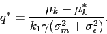
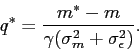
5.3.2 Effects of Belief Dispersion
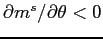
We now turn to analyze how changes in ![]() affect
the equilibrium stock price. We derive the expression of
affect
the equilibrium stock price. We derive the expression of
![]() from Equation (15) as follows.
from Equation (15) as follows.
Let ![]() and
and ![]() be the
average
be the
average ![]() and the average extent of manipulation
perceived by the investors participating in the stock market.
Thus,
and the average extent of manipulation
perceived by the investors participating in the stock market.
Thus,
Combining this and
![]() , we obtain
, we obtain
![]() , which implies that
the participating investors are on average more optimistic about
reporting quality than the investor population. Using Equation
(14), we write the
equilibrium stock price as a function of
, which implies that
the participating investors are on average more optimistic about
reporting quality than the investor population. Using Equation
(14), we write the
equilibrium stock price as a function of ![]() :
:
When there is limited market participation, the equilibrium stock price is determined by the average degree of manipulation perceived by market participants. We have the following results regarding the impact of belief dispersion on price dynamics under limited participation.
Lemma 3 Suppose that the full-participation condition (13) is not satisfied. The following results hold under limited market participation.
- The average
 perceived by market
participants increases with the dispersion in investor beliefs
about manipulation, i.e.,
perceived by market
participants increases with the dispersion in investor beliefs
about manipulation, i.e.,
 .
. - The average level of manipulation perceived by market
participants decreases with the dispersion in investor beliefs
about manipulation, i.e.,
 .
. - The equilibrium stock price increases with the dispersion in
investor beliefs about manipulation, i.e.,
 .
.
Proof: See Appendix C.
Let us consider the effect of increasing ![]() when there is limited participation. A greater dispersion is
associated with a broader spectrum of beliefs. Unlike the case of
full market participation where an increase in belief dispersion
equally affects optimistic investors and pessimistic investors, the
effect of an increased
when there is limited participation. A greater dispersion is
associated with a broader spectrum of beliefs. Unlike the case of
full market participation where an increase in belief dispersion
equally affects optimistic investors and pessimistic investors, the
effect of an increased ![]() on market participants
is not symmetrical under limited participation. Because investors
who are sufficiently pessimistic about financial reporting
credibility do not hold stocks in the first place, an increase in
belief dispersion essentially raises the level of market optimism
about reporting quality. That is, the average degree of
manipulation perceived by market participants is lower when
on market participants
is not symmetrical under limited participation. Because investors
who are sufficiently pessimistic about financial reporting
credibility do not hold stocks in the first place, an increase in
belief dispersion essentially raises the level of market optimism
about reporting quality. That is, the average degree of
manipulation perceived by market participants is lower when
![]() is larger.
is larger.
The intuition for an increased equilibrium stock price in response to an increase in belief dispersion is straightforward. As investors participating in the market become more optimistic about firm value on average, the increased market optimism drives up the equilibrium stock price.
Proposition 5 Suppose that the full-participation
condition (13) is
not satisfied, price volatility (![]() ) and equity
premium (
) and equity
premium (![]() ) increase with manipulation uncertainty
(
) increase with manipulation uncertainty
(![]() ).
).
Proof: See Appendix C.
Analogous to the representative-agent economy, as investors'
uncertainty about manipulation ![]() adds an
extra risk component to firm value and asset payoffs, price
volatility and equity premia both increase with the manipulation
uncertainty as in the representative-investor case.
adds an
extra risk component to firm value and asset payoffs, price
volatility and equity premia both increase with the manipulation
uncertainty as in the representative-investor case.
6 Equilibrium Participation Rate
It has been well documented that a significant proportion of the U.S. households do not participate in the stock markets. For instance, the 2005 Survey of Consumer Finances shows that about 50% of U.S. households own stocks or stock mutual funds (including holdings in their retirement accounts). Several models have been proposed to explain why limited market participation may exist (Allen and Gale (1994), Williamson (1994), Haliassos and Bertaut (1995), Vissing-Jorgensen (2002), and Yaron and Zhang (2000)). Those models focus on how entry costs and liquidity needs can cause limited market participation. Closest to ours is Cao et al. (2005), which studies uncertainty-averse investors who evaluate an investment strategy according to the expected utility under the worst case probability distribution in a set of prior distributions. When uncertainty dispersion is large in their model, investors with high uncertainty choose not to participate in the stock market, resulting in limited market participation. We offer an alternative explanation for limited market participation based on the existence of earnings management, without behavioral utility specifications. In addition, our model provides insight into how accounting standards and corporate governance policies influence market participation.
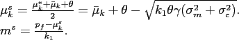
Let ![]() be the equilibrium participation rate in
our model:
be the equilibrium participation rate in
our model:
We re-write Equation (15)
as a function of ![]() :
:
We solve for the equilibrium participation rate in closed form as follows.
6.1 Corporate Governance and Market Participation
To gain insight on policy-related issues, it is of interest to
examine the impact of manipulation costs on market participation.
When the cost of manipulation (![]() ) varies due to
governance policy alterations, each participating investor changes
the size of their stock holding (the intensive margin), and
therefore the set of investors participating in the market (the
extensive margin) must change as well for the market to clear.
Using Equation (11),
we write the individual demand of each market participant (for a
given
) varies due to
governance policy alterations, each participating investor changes
the size of their stock holding (the intensive margin), and
therefore the set of investors participating in the market (the
extensive margin) must change as well for the market to clear.
Using Equation (11),
we write the individual demand of each market participant (for a
given ![]() ) as
) as
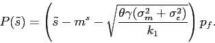
In Figure 2,
the individual demand (![]() ) is described as the line
) is described as the line
![]() . It depicts how the optimal holding of
market participants varies with their perceived
. It depicts how the optimal holding of
market participants varies with their perceived ![]() . The total demand by market participants is thus
represented by the shaded area below the
. The total demand by market participants is thus
represented by the shaded area below the ![]() line,
which must equal to the total quantity of stock outstanding
(normalized to 1) for the stock market to clear. In
other words, the price
line,
which must equal to the total quantity of stock outstanding
(normalized to 1) for the stock market to clear. In
other words, the price ![]() (which shifts the
(which shifts the
![]() line up and down in a parallel manner,
which can be seen from the above equation) adjusts so that the
shaded area is equal to 1.
line up and down in a parallel manner,
which can be seen from the above equation) adjusts so that the
shaded area is equal to 1.
As a high value of ![]() represents an optimism
in firm performance for a given financial report, the slope of the
individual demand curve
represents an optimism
in firm performance for a given financial report, the slope of the
individual demand curve ![]() (that is,
(that is,
![]() ) determines the marginal increase in demand due to investor
optimism, and thus also determines how demand is distributed across
market participants with differential beliefs. If the
) determines the marginal increase in demand due to investor
optimism, and thus also determines how demand is distributed across
market participants with differential beliefs. If the ![]() line is steep, a small number of the most optimistic
investors can demand a large volume of stock, thus driving up the
stock price sufficiently high to force out other investors. A small
fraction of investors fully absorb the market in this case. With a
more flat
line is steep, a small number of the most optimistic
investors can demand a large volume of stock, thus driving up the
stock price sufficiently high to force out other investors. A small
fraction of investors fully absorb the market in this case. With a
more flat ![]() line, the equilibrium price adjusts so
that a greater proportion of investors are induced to hold stocks
and clear the market.
line, the equilibrium price adjusts so
that a greater proportion of investors are induced to hold stocks
and clear the market.
There are two conflicting forces that determine how the slope of
the ![]() line varies with
line varies with ![]() .
Consider an increase in
.
Consider an increase in ![]() due to tightened corporate
governance policies. On the one hand, the difference in the belief
of
due to tightened corporate
governance policies. On the one hand, the difference in the belief
of ![]() is translated less into the difference
in investor optimism in reporting and firm value (i.e.,
is translated less into the difference
in investor optimism in reporting and firm value (i.e.,
![]() decreases). A large value of
decreases). A large value of ![]() implies a small
value of
implies a small
value of ![]() , which represents an optimistic view of the
firm performance given the report (recall that
, which represents an optimistic view of the
firm performance given the report (recall that ![]() ). When
). When ![]() is large, the degree of
manipulation becomes small, and a large heterogeneity in the
beliefs of
is large, the degree of
manipulation becomes small, and a large heterogeneity in the
beliefs of ![]() does not lead to a large
heterogeneity in the perceived manipulation
does not lead to a large
heterogeneity in the perceived manipulation ![]() . Thus
the demand heterogeneity across investors with different beliefs of
. Thus
the demand heterogeneity across investors with different beliefs of
![]() becomes small. This flattens the
becomes small. This flattens the
![]() line. On the other hand, the reduced
manipulation uncertainty (
line. On the other hand, the reduced
manipulation uncertainty (
![]() ) causes the
demand to be more sensitive to the information and investor
beliefs. This effect makes the
) causes the
demand to be more sensitive to the information and investor
beliefs. This effect makes the ![]() line steeper. It
turns out that the first effect, that is, the effect of the reduced
relevance of optimism, dominates when
line steeper. It
turns out that the first effect, that is, the effect of the reduced
relevance of optimism, dominates when
![]() . Therefore,
the
. Therefore,
the ![]() line becomes flatter when
line becomes flatter when ![]() increases. For the market to clear, the price has to adjust so that
increases. For the market to clear, the price has to adjust so that
![]() increases (to
increases (to ![]() on the
on the ![]() line in Figure 2). The
following lemma summarizes the main result on the relationship
between market participation and manipulation costs.
line in Figure 2). The
following lemma summarizes the main result on the relationship
between market participation and manipulation costs.
Figure 2: Effects of![]()
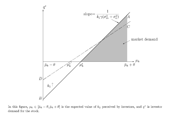
Lemma 4 Suppose that the full-participation
condition (Equation 13) is not
satisfied and
![]() holds. Then
the equilibrium participation rate is increasing in
holds. Then
the equilibrium participation rate is increasing in ![]() , i.e.,
, i.e.,
![]() .
.
Proof: See Appendix C.
When ![]() is large compared to the relative
uncertainty associated with
is large compared to the relative
uncertainty associated with ![]() , the effect of
decreased manipulation uncertainty is dominated by that of the
reduced importance of investor optimism. The demand is less
sensitive to investor beliefs (
, the effect of
decreased manipulation uncertainty is dominated by that of the
reduced importance of investor optimism. The demand is less
sensitive to investor beliefs (![]() ) when
) when
![]() increases. The intensive margin
consequently falls for each investor initially participating in the
market, and thus the extensive margin must increase to clear the
market. In a nutshell, market participation rate increases in
response to an increased
increases. The intensive margin
consequently falls for each investor initially participating in the
market, and thus the extensive margin must increase to clear the
market. In a nutshell, market participation rate increases in
response to an increased ![]() associated with tightened
governance policies. The increasing stringency of corporate
governance and accounting standards may have played a role in the
contemporaneous run-up of market participation rates in the recent
years.
associated with tightened
governance policies. The increasing stringency of corporate
governance and accounting standards may have played a role in the
contemporaneous run-up of market participation rates in the recent
years.
6.2 Belief Dispersion and Market Participation
The following lemma suggests a negative relationship between market participation and the dispersion in investor beliefs about earnings management.
Lemma 5 Suppose that the full-participation
condition (13) is
not satisfied, the equilibrium participation rate is decreasing in
the dispersion in investor beliefs about manipulation, i.e.,
![]() .
.
Proof: See Appendix C.
Under limited participation, investors sufficiently pessimistic about the credibility of reporting optimally choose not to invest in stocks. When investor beliefs about the extent of manipulation become more dispersed, investors who are in the market are more optimistic on average. As market participants on average have a more favorable view about firm value, stronger demand driven by market optimism raises the equilibrium stock price, forcing more pessimistic investors to withdraw from the market. The proportion of investors participating in the stock market therefore decreases as their perceptions about manipulation become more dispersed.
A few decades ago, most market participants were individual investors. Over time, equity markets have become more "institutionalized"; buyers have become largely institutions (e.g. pension funds, insurance companies, mutual funds, index funds, hedge funds, banks and various other financial institutions). Meanwhile, the stock market participation rate has trended upwards in the past few decades. The rise of institutional investors has brought with it a greater degree of homogeneity in market participants' perceptions of firm value, which may have contributed to the increased rates of market participation that occurred at the roughly same time.
7 Conclusion
We analyze a simple model of asset pricing under asymmetric information about earnings management. We consider an economy endowed with a given quantity of equity, and in which future dividends on the equity are stochastic. In order to boost share prices, managers have an incentive to portray unjustified future success and distort the information content of financial statements. Investors rationally extract information from possibly biased reports, but fail to perfectly infer the underlying states in equilibrium. We have shown in this paper that, by distinguishing between the cash flows received by equity holders and financial reports released by managers, and by allowing for learning about an unobservable degree of manipulation, it is possible to generate a representative agent model with rational behavior that is broadly consistent with several stylized facts in the financial markets.
One key feature of our model is that investors face information asymmetry regarding the extent of manipulation. Market uncertainty about the degree of manipulation can cause stock prices to move more than is warranted by changes in firm fundamentals. Risk-averse investors are compensated for increased volatility through higher returns on the stock, and demand a higher premium for bearing additional risk associated with their asset payoffs in equilibrium.
In addition, we study the implication of earnings management for stock market participation. Our model of manipulation endogenously gives rise to limited market participation when investors have heterogeneous views about the degree of manipulation. When the dispersion among investor beliefs about manipulation is sufficiently large, investors who are pessimistic about the credibility of financial reporting will consider the market price unjustified by firm value and optimally choose not to invest in stocks in equilibrium.
Our model allows us to derive a number of empirically relevant comparative static results on stock market participation. In particular, our model yields implications of how accounting standards and corporate governance policies influence market participation rates. In association with more stringent governance regimes, the impact of increased manipulation cost on market participation is determined by how demand for stocks is distributed across investors with heterogeneous beliefs. If the demand is sensitive to investor beliefs of manipulation, a small portion of the most optimistic investors can demand a large volume of stocks, thus driving up the stock price sufficiently high to force out other investors. If investors' demand does not vary much with their beliefs, the equilibrium stock price must induce a large proportion of investors to fully absorb the market.
Increasing the cost of manipulating financial statements has two conflicting effects on the distribution of investor demand for stocks. On the one hand, the degree of manipulation is reduced, and thus the demand heterogeneity across investors with differential beliefs becomes smaller. On the other hand, a decreased degree of manipulation brings with it reduced uncertainty of manipulation, causing investors' demand to be more sensitive to their beliefs. When the cost of manipulation is large, the first effect, that is, the effect of reduced importance of investor optimism, dominates, individual demand is less sensitive to investor beliefs when the manipulation cost increases. As a result of the decreased individual demand by market participants (intensive margin), the equilibrium participation rate (extensive margin) increases to clear the market. The increasing stringency of corporate governance and accounting standards may have contributed to the contemporaneous run-up of market participation rates in the recent years.
The market participation rate also decreases with the dispersion in investor beliefs about manipulation in our model. Under limited participation, when investor beliefs about the extent of manipulation become more dispersed, market participants on average have a more favorable view about the accountability of managers' reports and thus the financial condition of the firm. The increased market optimism drives up the equilibrium market price, forcing more investors to withdraw from the market. The rise of institutional investors and the associated greater degree of investor homogeneity may have played a role in the increase in market participation over the past few decades.
Bibliography
Allen, F. and D. Gale. (1994). "Limited Market Participation and Volatility of Asset Prices," American Economic Review, 84: 933-955.
Cao, H. H., T. Wang, and H. H. Zhang. (2005). "Model Uncertainty, Limited Market Participation, and Asset Prices," Review of Financial Studies, 18(4): 1219-1251.
Cecchetti, S. G., P. Lam, and N. Mark. (2000). "Asset Pricing with Distorted Belief: Are Equity Returns Too Good to Be True?" American Economic Review, 4: 787-805.
Detemple, J. B. (1986) "Asset Pricing in a Production Economy with Incomplete Information," The Journal of Finance, 41: 381-391.
Fischer, P. E. and R. E. Verrecchia. (1978) "Reporting Bias," Accounting Review, 75:229-245.
Goldman, E. and S. L. Slezak. (2006). "An Equilibrium Model of Incentive Contracts in the Presence of Information Manipulation" Journal of Financial Economics 80, 603-626.
Grossman, S. J. (1976). "On the Efficiency of Competitive Stock Markets where Traders Have Diverse Information," Journal of Finance, 31: 573-585.
Guttman, I., O. Kadan, and E. Kandel. (2006) "A Rational Expectations Theory of Kinks in Financial Reporting," Accounting Review 81(4): 811-848.
Haliassos, M. and C. Bertaut. (1995). "Why Do So Few Hold Stocks?" The Economic Journal, 105: 1110-1129.
Harrison, J. M. and D. M. Kreps. (1978). "Speculative Investor Behavior in a Stock Market with Heterogeneous Expectations," The Quarterly Journal of Economics, 92(2): 323-336.
Kwon, I. and E. Yeo. "Overstatement and Rational Expectations," Working paper, SUNY at Albany and Korea Institute of Finance, 2008. Available at http://www.albany.edu/econ/Research/2008/Overstatement.pdf.
LeRoy, S. and R. Porter. (1981). "The Present Value Relation: Tests Based on Variance Bounds," Econometrica, 49: 555-574.
Lucas, R. E. (1978) "Asset Prices in an Exchange Economy," Econometrica, 46:1429-1445.
Riley, J. G. (1979). "Informational Equilibrium," Econometrica, 47: 331-359.
Scheinkman, J. A. and W. Xiong. (2003). "Overconfidence and Speculative Bubbles," Journal of Political Economy, 111(6): 1183-1219.
Shiller, R. J. (1981) "Do Stock Prices Move Too Much To Be Justified By Subsequent Changes in Dividends?," American Economic Review, 71: 421-436.
Stein, J. C. (1989). "Efficient Capital Markets, Inefficient Firms: A Model of Myopic Corporate Behavior," Quarterly Journal of Economics, 104: 655-669.
Sun, B. (2010). "Asset Returns with Earnings Management," International Finance Discussion Paper, Federal Reserve Board.
Vissing-Jorgensen, A. (2002). "Limited Asset Market Participation and the Elasticity of Intertemporal Substitution," Journal of Political Economy, 110(4): 825-853.
Wang, J. (1993) "A Model of Intertemporal Asset prices under Asymmetric Information," Review of Economic Studies, 60: 249-282.
Williamson, S. (1994). "Liquidity and Market Participation," Journal of Economic Dynamics and Control, 18: 629-670.
Yaron, A. and H. H. Zhang. (2000). "Fixed Costs and Asset Market Participation," Revista De Analisis Economico, 15: 89-109.
Appendix
A Equilibrium Stock Price Under Truthful Reporting
Proof of Proposition 1: Given the
manager's report ![]() , the expected terminal
wealth of investors when they purchase
, the expected terminal
wealth of investors when they purchase ![]() shares of the
firm's stock and
shares of the
firm's stock and ![]() shares of the riskless asset
is
shares of the riskless asset
is
| (18) |
Substituting
![]() into (18), investors'
expected wealth can be expressed as
into (18), investors'
expected wealth can be expressed as
![\begin{displaymath} E[W\vert\tilde s]=\tilde s q + \displaystyle \frac{W_0-p^*q}{p_f}. \end{displaymath}](img323.gif) |
(19) |
The variance of investors' terminal wealth given the manager's report is
| (20) |
Plugging Equation (19) and (20) into investors' objective function (Equation 2), we obtain
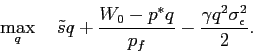 |
(21) |
Taking the derivative of Equation (21) with respect to
![]() , we obtain the first-order condition for
the investors' problem:
, we obtain the first-order condition for
the investors' problem:
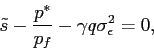
which leads to the expression of the share of the stock investors purchase in the equilibrium:
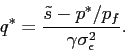
The market clears when
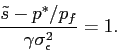
We obtain the following equilibrium pricing function.
Proof of Lemma 1:
![\begin{align*} Var[p^*] &= Var[\displaystyle (\tilde s - \gamma \sigma^2_\epsilon)p_f] \ &=\displaystyle p^2_f(\sigma^2_\epsilon+\sigma^2_y).\ e^*&= E\left[\frac{y}{p^*} \bigg \vert \tilde s \right] -r_f \ &= \displaystyle \frac{1}{p_f} \bigg\{ E\bigg[ \frac{y}{\tilde s -\gamma\sigma^2_\epsilon} \bigg] -1\bigg\}.\ \end{align*}](img331.gif)
It is straightforward to see that ![]() and
and
![]() are both increasing in
are both increasing in
![]() .
. ![]()
B Stock Price with Manipulation: Perfect Information
B.1 Without Manipulation Costs
We first consider the case where there is no cost involved in
manipulating earnings reports, i.e., ![]() . The
only equilibrium in this case is that the firm's price is
independent of the report, and the reporting function is
indetermined.
. The
only equilibrium in this case is that the firm's price is
independent of the report, and the reporting function is
indetermined.
Lemma 6 When manipulation is costless to the manager, the equilibrium share price
If the manager does not incur any cost when falsifying financial records, the manager will always report the earnings that would generate the highest share price possible. Anticipating the manager's reporting incentive, the best response of investors is to discard the report completely and price the firm based on the unconditional expected earnings.
B.2 With Manipulation Costs
We now turn to analyze the case where manipulating reports incurs a
personal cost to the manager,
![]() . The cost function of
earnings management (i.e., the value of
. The cost function of
earnings management (i.e., the value of ![]() and
and
![]() ) is public information available to
investors.
) is public information available to
investors.
We solve the problem following the "guess and verify" approach.
We conjecture that the equilibrium pricing function ![]() is linear in earnings reports
is linear in earnings reports
![]() . We will
check whether the equilibrium value of prices is in fact linear by
imposing the market clearing condition.
. We will
check whether the equilibrium value of prices is in fact linear by
imposing the market clearing condition.
Lemma 7 In a setting where the manager has
discretion to manipulate earnings reports, and the cost of
manipulation is publicly known to investors, the firm's stock price
given the manager's report ![]() can be
expressed as
can be
expressed as
![]()
where ![]() is the equilibrium reporting strategy
of the manager
is the equilibrium reporting strategy
of the manager
![]()
Proof: With the conjectured price function, the first-order condition for the manager's problem (1) yields
| (22) |
and therefore
| (23) |
Given the manager's report, investors form their expectation of the future wealth as follows:
![\begin{eqnarray*} E[W\vert\tilde s] &=& E[y\vert \tilde s] q + q_f \ &=& \displaystyle E[\tilde s- m - \epsilon]q+\frac{W_0-p q}{p_f}. \ Var[W\vert\tilde s] &=& q^2 Var[y\vert \tilde s] = \displaystyle q^2 \sigma^2_\epsilon. \end{eqnarray*}](img349.gif)
Substituting these into the investors' objective function (2), the investors' problem is given by8
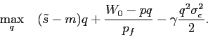
The optimization problem of investors can be characterized by the following first-order condition.
Solving for the optimal share of the stock investors are willing to hold, we arrive at the following expression.
 |
(24) |
When the market clears, it must be equal to the quantity of stock available, which is normalized to 1. Thus,
The stock price that clears the market is
Therefore, the price is in fact linear in ![]() ,
and matching the coefficients with the conjecture
,
and matching the coefficients with the conjecture
![]() yields the
solutions
yields the
solutions
and
where ![]() is given by
is given by
Because the manipulation component in the report (![]() ) is perfectly filtered out by investors, the manager's
opportunity to manipulate does not affect the degree of market
uncertainty about future fundamentals (
) is perfectly filtered out by investors, the manager's
opportunity to manipulate does not affect the degree of market
uncertainty about future fundamentals (![]() ). The
dynamics of prices and required returns are identical to the case
in the absence of opportunities to manipulate.
). The
dynamics of prices and required returns are identical to the case
in the absence of opportunities to manipulate.
Proposition 6 In a setting where
the manager manipulates earnings reports subject to a cost function
that is public information, price volatility (![]() ) and excess returns (
) and excess returns (![]() ) are identical to
those without possibilities of manipulation.
) are identical to
those without possibilities of manipulation.
Proof:
![\begin{align*} Var[p]&=(\sigma_y^2+\sigma_\epsilon^2) p_f^2.\ e &= E\left[\frac{y}{p} \bigg \vert \tilde s \right] -r_f \ &= \displaystyle \frac{1}{p_f} \bigg\{ E\bigg[ \frac{y}{\tilde s -m-\gamma\sigma^2_\epsilon}\bigg] -1\bigg\} \end{align*}](img370.gif)
where
C Proofs
Proof of Proposition 3:
![\begin{align*} Var[p] -Var[p^*] &=\left(\sigma_y^2 + \sigma_\epsilon^2 + \frac{\sigma_k^2}{k_1^2}\right)p_f^2 - (\sigma_y^2 + \sigma_\epsilon^2 )p_f^2 =\frac{\sigma^2_k p^2_f}{k_1^2}>0\ \frac{\partial Var[p]}{\partial \sigma^2_k} &= \frac{p^2_f}{k^2_1}>0. \quad\Box \end{align*}](img372.gif)
Proof of Proposition 4: When investors only know about the distribution of the manipulation cost but not the exact value, the equity premium on the firm's stock is
![\begin{eqnarray*} e & \equiv & E[R\vert \tilde s] - r_f \ &=&\displaystyle E\bigg[ \frac{y}{\tilde s -\mu_m -\gamma (\sigma^2_\epsilon + \sigma^2_m)} \bigg] - r_f \end{eqnarray*}](img373.gif)
We first rewrite
![]() by the law of
iterated expectations, and reduce the comparison of
by the law of
iterated expectations, and reduce the comparison of
![]() to the comparison of
to the comparison of
![]() in the cases with and without
manipulation.
in the cases with and without
manipulation.
In the absence of manipulation, we have
In the presence of manipulation, there is one additional random
variable ![]() . Thus,
. Thus,
We show below that
| (25) |
and the following relationship automatically follows:
| (26) |
Then since ![]() is higher with the
opportunity to manipulate than without the opportunity,
is higher with the
opportunity to manipulate than without the opportunity,
![]() and thus
and thus ![]() are higher in the presence of manipulation.
are higher in the presence of manipulation.
Now we turn to show that Equation (25) holds. For
notational convenience, let ![]() . We know
that
. We know
that ![]() and
and ![]() is convex in
is convex in
![]() , where
, where ![]() is defined
as
is defined
as
According to Jensen's inequality,
![]() . That is,
. That is,
Thus Equation (26)
follows. Therefore, the equity premium on the firm's stock
(![]() ) is higher under earnings management than
under truthful reporting, and it is increasing in
) is higher under earnings management than
under truthful reporting, and it is increasing in ![]() .
. ![]()
Proof of Lemma 2: We rewrite the pricing equation (14) as
Taking derivative with respect to ![]() ,
,
Given that ![]() ,
,
![]() as long as
as long as
![]() . We know
that
. We know
that
When
![]() , we have
, we have
![]() , and thus
, and thus
![]() .
. ![]()
Proof of Lemma 3 (1):
 . As Equation (13)
is not satisfied,
. As Equation (13)
is not satisfied,
holds under limited participation. Thus,
Proof of Lemma 3 (2):
Proof of Lemma 3 (3):
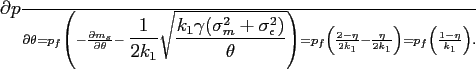
As ![]() holds under limited participation,
holds under limited participation,
![]() holds as
well.
holds as
well. ![]()
Proof of Proposition 5:
![\begin{displaymath} Var[p] = p^2_f \left(\sigma^2_y+\sigma^2_\epsilon+\frac{\sigma^2_k}{k^2_1}\right). \end{displaymath}](img417.gif)
As
![]() ,
, ![]() is increasing in
is increasing in ![]() .
.
We first show below that
![\begin{align*} \displaystyle \frac{\partial m^*}{\partial \sigma^2_k} &= -\frac{1}{k_1} \frac{\partial \mu^*_k}{\partial \sigma^2_k} \ &= -\frac{1}{k_1}\bigg[ -\frac{1}{k_1}\sqrt{\frac{\theta \gamma}{k_1(\sigma^2_\epsilon+\sigma^2_k/k^2_1)}} \bigg]\ &= \frac{1}{k^2_1}\sqrt{\frac{\theta \gamma}{k_1(\sigma^2_\epsilon+\sigma^2_k/k^2_1)}}\ &>0. \end{align*}](img423.gif)
As ![]() is increasing in
is increasing in ![]() ,
, ![]() is also increasing in
is also increasing in ![]() .
. ![]()
Proof of Lemma 4: Let
![]() . Then
. Then
![]() can be rewritten as
can be rewritten as
Taking derivative of
When
Proof of Lemma 5:
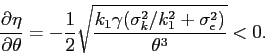
Footnotes
1. I gratefully acknowledge Toshi Mukoyama for his help. I thank John Ammer, Mark Carey, Steve Sharpe, Missaka Warusawitharana, and seminar participants at the Federal Reserve Board and Midwest Theory Conference for comments and suggestions. The views expressed herein are the author's and do not necessarily reflect the opinions of the Board of Governors of the Federal Reserve System. Return to text
2. Contact: Division of International Finance, Board of Governors of the Federal Reserve, Mail Stop 44, 20th Street and Constitution Avenue, Washington, DC 20551. [email protected]. (202)452-2343. Return to text
3. This paper considers a broad notion of "earnings management" in that it includes any manipulation of current economic performance that generates informational asymmetry between managers and investors. For a broad review of empirical evidence on earnings management, see Healy and Wahlen (1999). Return to text
4. For simplification, we adopt this functional form of manipulation costs to make the optimization problem concave and well defined. The quadratic functional form can be interpreted as a local approximation of a more general convex function. Return to text
5. Later we will show that the distribution
of ![]() conditional on
conditional on ![]() follows
a normal distribution. Return to
text
follows
a normal distribution. Return to
text
6. This equilibrium is similar to Riley (1979), Stein (1989), Goldman and Slezak (2006), and Guttman et al. (2006). Return to text
7. Because ![]() and
and
![]() follow normal distributions, the
distribution of
follow normal distributions, the
distribution of ![]() conditional on
conditional on ![]() is a linear combination of normal distribution and is
thus also a normal distribution. Return
to text
is a linear combination of normal distribution and is
thus also a normal distribution. Return
to text
8. Because ![]() and
and
![]() follow normal distributions, the
distribution of
follow normal distributions, the
distribution of ![]() conditional on
conditional on ![]() is a linear combination of normal distribution and is
thus also a normal distribution. Return
to text
is a linear combination of normal distribution and is
thus also a normal distribution. Return
to text
This version is optimized for use by screen readers. Descriptions for all mathematical expressions are provided in LaTex format. A printable pdf version is available. Return to text