Skip to: [Printable Version (PDF)] [Bibliography] [Footnotes]

Finance and Economics Discussion Series: 2005-08 Screen Reader version*

Real-time Model Uncertainty in the United States:
the Fed from 1996-2003¹

Robert J. Tetlow and Brian Ironside.

Federal Reserve Board

December 2005

Keywords: monetary policy, uncertainty, real-time analysis.

Abstract:

We study 30 vintages of FRB/US, the principal macro model used by the Federal Reserve Board staff for forecasting and policy analysis. To do this, we exploit archives of the model code, coefficients, baseline databases and stochastic shock sets stored after each FOMC meeting from the model's inception in July 1996 until November 2003. The period of study was one of important changes in the U.S. economy with a productivity boom, a stock market boom and bust, a recession, the Asia crisis, the Russian debt default, and an abrupt change in fiscal policy. We document the surprisingly large and consequential changes in model properties that occurred during this period and compute optimal Taylor-type rules for each vintage. We compare these optimal rules against plausible alternatives. Model uncertainty is shown to be a substantial problem; the efficacy of purportedly optimal policy rules should not be taken on faith. We also find that previous findings that simple rules are robust to model uncertainty may be an overly sanguine conclusion.

JEL Classifications: E37, E5, C5, C6.

Introduction

Policy makers face a formidable problem. They must decide on a policy notwithstanding considerable ambiguity about the proper course of action. Monetary policy makers in particular need to make decisions on a timely basis in an environment where the data are rarely authoritative on the state of the world. For guidance, they turn to models, but models too have their foibles. Both in academia and within central banks, the models in use today differ substantially from those of yesteryear. The policy prescriptions that come from these models also differ, and often in ways that could have important consequences for economic outcomes.

This paper considers, measures and evaluates real-time model uncertainty in the United States. In particular, we study 30 vintages of the Board of Governors' workhorse macroeconomic model, FRB/US, that were used extensively for forecasting and policy analysis at the Fed from the model's inception in July 1996 until November 2003. To do this, we exploit archives of the model code, coefficients, databases and stochastic shock sets for each vintage. The choice of the model is not incidental: by working with the FRB/US model, we isolate the policy issues and forecast outcomes that actually affected the Fed staff's modeling decisions over time. The period of study was one of remarkable change in the U.S. economy with a productivity boom, a stock market boom and bust, a recession, the Asia crisis, the Russian debt default, corporate governance scandals and an abrupt change in fiscal policy. There were also 23 changes in the intended federal funds rate, 7 increases and 16 decreases.

Armed with this archive, we do four things: First, we examine the real-time data. Second, we document the changes in the model properties-a surprisingly large and consequential set, it turns out-and identify the economic events that contributed to them. Third, we compute optimal Taylor-type rules for each vintage. And fourth, we compare the performance of these ex ante optimal rules against alternative rules, including an ex post optimal rule, and the original Taylor (1993) specification. From this, we draw conclusions about model uncertainty and its implications for policy design. It turns out that model uncertainty is quantitatively large and important, even over the short period studied here. In this regard, our findings are consistent with those of Sargent, Williams and Zha (2005), although our approach is very different.

This exercise goes a number of steps beyond previous contributions to the literature. One technique often used to study model uncertainty is the rival models method, where following the suggestion of McCallum (1988) a candidate policy rule is assessed for its performance across an entire set of rival models. The limitation is that it is far from obvious how to settle on the set of rival models. To date, the literature has used alternative models of relatively abstract economies compared in a laboratory environment. As a result, Levin et al. (1999) for example were susceptible to the criticism of Christiano and Gust (1999) that their analysis of the robustness properties of simple Taylor-type rules was undermined by the similarity of the models they chose.² Our real-time analysis avoids this problem by basing the rival models on the decisions of the Board of Governors' staff, conditional on the issues and questions that the staff faced. Thus the set is a plausible one. ³

The current paper also goes beyond the literature on parameter uncertainty. That literature assumes that parameters are random but the model is fixed over time; misspecification is simply a matter of sampling error.⁴ Model uncertainty is a thornier problem, in large part because it often does not lend itself to statistical methods of analysis. We explicitly allow the models to change over time in response not just to the data but to the economic issues of the day.⁵ Lastly, and most important, the analysis we provide derives from models that were actually used to advise on monetary policy decisions. To the best of our knowledge, no one has ever done this before.

The rest of this paper proceeds as follows. The second section begins with a discussion of the FRB/US model in generic terms, and the model's historical archives. The third section compares model properties by vintage. To do this, we document changes in real-time "model multipliers" and compare them with their ex post counterparts. The succeeding section computes optimized Taylor-type rules and compares these to commonly accepted alternative policies in a stochastic environment. The fifth section examines the stochastic performance of candidate rules for two selected vintages, the February 1997 and November 2003 models. A sixth and final section sums up and concludes.

Thirty vintages of the FRB/US model and the data

The real-time data

In describing model uncertainty, it pays to start at the beginning; in present circumstances, the beginning is the data. It is the data, and the staff's view of those data, that determined how the first vintage of FRB/US was structured. And it is the surprises from those data and how they were interpreted as the series were revised and extended with each successive vintage that conditioned the model's evolution. To that end, in this subsection we examine key data series by vintage. We also provide some evidence on the model's forecast record during the period of interest. And we reflect on the events of the time, the shocks they engendered, and the revisions to the data. Our treatment of the subject is subjective-it comes, in part, from the archives of the FRB/US model-and incomplete. It is beyond the scope of this part of the paper to provide an comprehensive survey of data revisions over the period from 1996 to 2003; fortunately, however, Anderson and Kliesen (2005) provide just such a summary and we borrow in places from their work.

Figure 2.1 shows the four-quarter growth rate of the GDP price index, for selected vintages. (Note we show only real-time historical data because of rules forbidding the publication of FOMC-related data more recent than in the last five years.) The inflation rate moves around some, but the various vintages for the most part are highly correlated. In any event, our reading of the literature is that data uncertainty, narrowly defined to include revisions of published data series, is not a first-order source of problems for monetary policy design; see, e.g., Croushore and Stark (2001). Figure 2.2 shows the more empirically important case of model measures of growth in potential non-farm business output.⁶

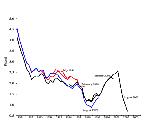
**Figure 2.1:** Real-time 4-quarter GDP price inflation (selected vintages)

**Figure 2.2:** Real-time 4-quarter non-farm potential business output growth

Unlike the case of inflation, potential output growth is a latent variable the definition and interpretation of which depends on model concepts. What this means is the historical measures of potential are themselves a part of the model, so we should expect significant revisions.⁷ Even so, the magnitudes of the revisions shown in Figure 2.2 are truly remarkable. The July 1996 vintage shows growth in potential output of about 2 percent. For the next several years, succeeding vintages show both higher potential output growth rates and more responsiveness to the economic cycle. By January 2001, growth in potential was estimated at over 5 percent for some dates, before subsequent changes resulted in a path that was lower and more variable. Why might this be? Table 1 reminds us about how extraordinary the late 1990s were. The table shows selected FRB/US model forecasts for the four-quarter growth in real GDP, on the left-hand side of the table, and PCE price inflation, on the right-hand side, for the period for which public availability of the data are not restricted.⁸ The table shows the substantial underprediction of GDP growth over most of the period, together with a underpredictions of PCE inflation.

Table 1 Four-quarter growth in real GDP and PCE prices: selected FRB/US model forecasts
forecast date	Real GDP forecast	Real GDP data	Real GDP data - forecast*	PCE prices forecast	PCE prices data	PCE prices data - forecast*
July 1996	2.2	4.0	1.8	2.3	1.9	-0.4
July 1997	2.0	3.5	1.5	2.4	0.7	-1.6
Aug. 1998	1.7	4.1	2.4	1.5	1.6	0.1
Aug. 1999	3.2	5.3	2.1	2.2	2.5	0.3
Aug. 2000	4.5	0.8	-3.7	1.8	1.5	-0.3
*4Q growth forecasts from the vintage of the year shown; e.g. for GDP in July 1996,
forecast =100*(GDP[1997:Q2]/GDP[1996:Q2]-1), compared against the "first final"
data contained in the database two forecasts hence. So for the same example, the
first final is from the November 1997 model database.

The most recent historical measures shown in Figure 2.2 are for the August 2002 vintage, where the path for potential output growth differs in two important ways from the others. The first way is that it is the only series shown that is less optimistic than earlier ones. In part, this reflects the onset of the 2001 recession. The second way the series differs is in its volatility over time. This is a manifestation of the ongoing evolution of the model in response to emerging economic conditions. In its early vintages, the modeling of potential output in FRB/US was traditional for large-scale econometric models, in that trend labor productivity and trend labor input, were based on exogenous split time trends. In essence, the model took the typical Keynesian view that nearly all shocks affecting aggregate output were demand-side phenomena. Then, as under-predictions of GDP growth were experienced, without concomitant underpredictions in inflation, these priors were updated. The staff began adding model code to allow the supply side of the model to respond to output surprises by projecting forward revised profiles for productivity growth. What had been an essentially deterministic view of potential output was evolving into a stochastic one.⁹

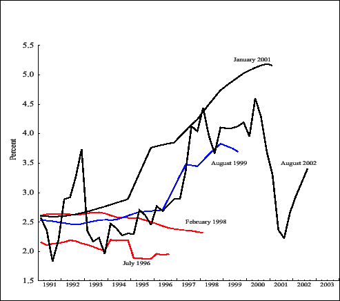
Further insight on the origins and persistence of these forecast errors can be gleaned from Figure 2.3 below, which focuses attention on a single year, 1996, and shows forecasts and "actual" four-quarter GDP growth, non-farm business potential output growth, and PCE inflation for that year. Each date on the horizontal axis corresponds with a database, so that the first observation on the far left of the black line is what the FRB/US model database for the 1996:Q3 (July) vintage showed for four-quarter GDP growth for1996. (The black line, is broken over the first two observations to indicate that some observations for 1996 were forecast data at the time; after the receipt of the advance release of the NIPA for 1996:Q4 on January 31, 1997, the figures are treated as data.) Similarly, the last observation of the same black line shows what the 2005:Q4 database has for historical GDP growth in 1996, given current concepts and measures. The black line shows that the model predicted GDP growth of 2.2 percent for 1996 as of July 1996; when the first final data for the 1996:Q4 were released on January 31, 1997, GDP growth for the year was 3.1 percent, a sizable forecast error of 0.8 percentage points. It would get worse. The black line shows that GDP growth was revised up in small steps and large jumps right up until late in 2003 and now stands at 4.4 percent; so by the (unfair) metric of current data, the forecast error from the July 1996 projection is a whopping 2.2 percentage points. Given the long climb of the black line, the revisions to potential output growth shown by the red line seem explicable, at least until about 2000. After that point, the emerging recession resulted in wholesale revisions of potential output growth going well back into history.

**Figure 2.3:** 4-quarter growth in 1996 for selected variables by vintage

The blue line shows that there was a revision in PCE inflation that coincided with substantial changes in both actual GDP and potential, in 1998:Q3. This reflects the annual revision of the NIPA data and with it some updates in source data.¹⁰

Comparing the black line, which represents real GDP growth, with the red line, which measures potential output growth, shows clearly the powerful influence that data revisions had on the FRB/US measures of potential.

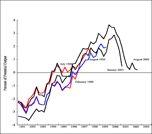
Despite the volatility of potential output growth, the resulting output gaps, shown in Figure 2.4, show considerable covariation, albeit with non-trivial revisions. This observation underscores the sometimes underappreciated fact that resource utilization (that is, output gaps or unemployment) is not the sole driver of fluctuations in inflation; other forces are also at work, including trend productivity which affects unit labor costs, and relative price shocks such those affecting food, energy and non-oil import prices.

**Figure 2.4:** Real-time GDP output gaps (selected vintages)

Description of the FRB/US model

The FRB/US model came into production in July 1996 as a replacement for the venerable MIT-Penn-SSRC (MPS) model that had been in use at the Board of Governors for many years.

The main objectives guiding the development of the model were that it be useful for both forecasting and policy analysis; that expectations be explicit; that important equations represent the decision rules of optimizing agents; that the model be estimated and have satisfactory statistical properties; and that the full-model simulation properties match the "established rules of thumb regarding economic relationships under appropriate circumstances" as Brayton and Tinsley (1996, p. 2) put it.

To address these challenges, the staff included within the FRB/US model a specific expectations block, and with it, a fundamental distinction between intrinsic model dynamics (dynamics that are immutable to policy) and expectational dynamics (which policy can affect). In most instances, the intrinsic dynamics of the model were designed around representative agents choosing optimal paths for decision variables facing adjustment costs.¹¹

Ignoring asset pricing equations for which adjustment costs were assumed to be negligible, a generic model equation would look something like:

$LaTex Encoded Math: \displaystyle \Delta x=\alpha(L)\Delta x+E_{t}\beta(F)\Delta x^{\ast}+c(x_{t-1}% -x_{t-1}^{\ast})+u_{t}$

(1)

where $\alpha(L)$ is a polynomial in the lag operator, i.e., $\alpha (L)z=a_{0}+a_{1}z_{t-1}+a_{2}z_{t-2}+\ldots$ and $\beta(F)$ is a polynomial in the lead operator. The term $\Delta x^{\ast}$ is the expected changes in target levels of the generic decision variable, , is an error-correction term, and is a residual. In general, the theory behind the model will involve cross-parameter restrictions on $\alpha(L),\beta(F)$ and . The point to be taken from equation (1) is that decisions today for the variable, will depend in part on past values and expected future values, with an eye on bringing toward its desired value, $x^{\ast},$ over time.

From the outset, FRB/US has been a significantly smaller model than was MPS, but it is still quite large. At inception, it contained some 300 equations and identities of which perhaps 50 were behavioral. About half of the behavioral equations in the first vintage of the model were modeled using formal specifications of optimizing behavior.¹² Among the identities are the expectations equations.

Two versions of expectations formation were envisioned: VAR-based expectations and perfect foresight. The concept of perfect foresight is well understood, but VAR-based expectations probably requires some explanation. In part, the story has the flavor of the Phelps-Lucas "island paradigm": agents live on different islands where they have access to a limited set of core macroeconomic variables, knowledge they share with everyone in the economy. The core macroeconomic variables are the output gap, the inflation rate and the federal funds rate, as well as beliefs on the long-run target rate of inflation and what the equilibrium real rate of interest will be in the long run. These variables comprise the model's core VAR expectations block. In addition they have information that is germane to their island, or sector. Consumers, for example, augment their core VAR model with information about potential output growth and the ratio of household income to GDP, which forms the consumer's auxiliary VAR. Two important features of this set-up are worth noting. First, the set of variables agents are assumed to use in formulating forecasts is restricted to a set that is much smaller than under rational expectations. Second, agents are allowed to update their beliefs, but only in a restricted way. In particular, for any given vintage, the coefficients of the VARs are taken as fixed over time, while agents' perceptions of long-run values for the inflation target and the equilibrium real interest rate are continually updated using simple learning rules.¹³

By definition, under perfect-foresight expectations, the information set is broadened to include all the states in the model with all the cross-equation restrictions implied by the model.

In this paper, we will be working exclusively with the VAR-based expectations version of the model. Typically it is the multipliers of this version of the model that are reported to Board members when they ask "what if" questions. This is the version that is used for forecasting and most policy analysis by the Fed staff, including, as Svensson and Tetlow (2005) demonstrate, policy optimization experiments.¹⁴ Thus, the pertinence of using this version of the model for the question at hand is unquestionable. What might be questioned, on standard Lucas-critique grounds, is the validity of the Taylor-rule optimizations carried out below. However, the period under study is one entirely under the leadership of a single Chairman, and we are aware of no evidence to suggest that there was a change in regime during this period. So as Sims and Zha (2004) have argued, it seems likely that the perturbations to policies encompassed by the range of policies studied below are not large enough to induce a change in expectations formation. Moreover, in an environment such as the one under study, where changes in the non-monetary part of the economy are likely to dwarf the monetary-policy perturbations, it seems safe to assume that private agents were no more rational with regard to their anticipations of policy than the Fed staff was about private-sector decision making.¹⁵ In their study of the evolution of the Fed beliefs over a longer period of time, Romer and Romer (2002), ascribe no role to the idea of rational expectations. Finally, what matters for this real-time study is that it is certainly the case that the Fed staff believed that expectations formation, as captured in the model's VAR-expectations block, could be taken as given and thus policy analyses not unlike those studied here were carried out. Later on we will have more to say about the implications of assuming VAR-based expectations for our results and those in the rest of the literature.

There is not the space here for a complete description of the model, a problem that is exacerbated by the fact that the model is a moving target. Readers interested in detailed descriptions of the model are invited to consult papers on the subject, including Brayton and Tinsley (1996), Brayton, Levin, Tryon and Williams (1997), and Reifschneider, Tetlow and Williams (1999). However, before leaving this section it is important to note that the structure of macroeconomic models at the Fed have always responded to economic events and the different questions that those events evoke, even before FRB/US. Brayton, Levin, Tryon and Williams (1997) note, for example, how the presence of financial market regulations meant that for years a substantial portion of the MPS model dealt specifically with mortgage credit and financial markets more broadly. The repeal of Regulation Q induced the elimination of much of that detailed model code. Earlier, the oil price shocks of the 1970s and the collapse of Bretton Woods gave the model a more international flavor than it had previously. We shall see that this responsiveness of models to economic conditions and questions continued with the FRB/US model in the 1990s.

The key features influencing the monetary policy transmission mechanism in the FRB/US model are the effects of changes in the funds rate on asset prices and from there to expenditures. Philosophically, the model has not changed much in this area: all vintages of the model have had expectations of future economic conditions in general, and the federal funds rate in particular, affecting long-term interest rates and inflation. From this, real interest rates are determined and this in turn affects stock prices and exchange rates, and from there, real expenditures. Similarly, the model has always had a wage-price block, with the same basic features: sticky wages and prices, expected future excess demand in the goods and labor markets influencing price and wage setting, and a channel through which productivity affects real and nominal wages. That said, as we shall see, there have been substantial changes over time in both (what we may call) the interest elasticity of aggregate demand and the effect of excess demand on inflation.

Over the years, equations have come and gone in reflection of the needs, and data, of the day. The model began with an automotive sector but this block was later dropped. Business fixed investment was originally disaggregated into just non-residential structures and producers' durable equipment, but the latter is now disaggregated into high-tech equipment and "other". The key consumer decision rules and wage-price block have undergone frequent modification over the period. On the other hand, the model has always had an equation for consumer non-durables and services, consumer durables expenditures, and housing. There has always been a trade block, with aggregate exports and non-oil and oil imports, and equations for foreign variables. The model has always had a three-factor, constant-returns-to-scale Cobb-Douglas production function with capital, labor hours and energy as factor inputs.

The archive and the data

Since its inception in July 1996, the FRB/US model code, the equation coefficients, the baseline forecast database, and the list of stochastic shocks with which the model would be stochastically simulated, have all been stored for each of the eight forecasts the Board staff conducts every year. It is releases of National Income and Product Accounts (NIPA) data that typically induce re-assessments of the model, so we elected to use four archives per year, or 30 in total, the ones immediately following NIPA preliminary releases.¹⁶

In what follows, we experiment with each vintage of model, comparing their properties in selected experiments. Consistent with the real-time philosophy of this endeavor, the experiments we choose are typical of those used to assess models by policy institutions in general and the Federal Reserve Board in particular. They fall into two broad classes. One set of experiments, model multipliers, attempts to isolate the behavior of particular parts of the model. A multiplier is the response of a key endogenous variable to an exogenous shock after a fixed period of time. An example is the response of the unemployment rate after eight quarters to a persistent increase in the federal funds rate. We shall examine several such multipliers. The other set of experiments judge the stochastic performance of the model and are designed to capture the full-model properties under fairly general conditions. So, for example, we will compute by stochastic simulation the optimal coefficients of a Taylor rule, conditional on a model vintage, a baseline database, and a set of stochastic shocks.¹⁷ We will then compare these optimal rules with other alternative rules and indeed other alternative worlds defined by the set of our model vintages.

Model multipliers have been routinely reported to and used by members of the FOMC. Indeed, the model's sacrifice ratio-about which we will have more to say below-was used in the very first FOMC meeting following the model's introduction.¹⁸ Similarly, model simulations of alternative policies have been carried out and reported to the FOMC in a number of memos and official FOMC documents.¹⁹

The archives document model changes and provide a unique record of model uncertainty. As we shall see, the answers to questions a policy maker might ask differ depending on the vintage of the model. The seemingly generic issue of the output cost of bringing down inflation, for example, can be subdivided into several more precise questions, including: (i) what would the model say is the output cost of bringing down inflation today?; (ii) what would the model of today say the output cost of bringing down inflation would have been in February 1997?; and (iii) what would the model have said in February 1997 was the output cost of disinflation at that time? These questions introduce a time dependency to the issue that rarely appears in other contexts.

The answers to these and other related questions depend on the model vintage. Here, however, the model vintage means more than just the model alone. Depending on the question, the answer can depend on the baseline; that is, on the initial conditions from which a given experiment is carried out. It can also depend on the way an experiment is carried out, and in particular on the policy rule that is in force. And since models are evaluated in terms of their stochastic performance, it can depend on the stochastic shocks to which the model is subjected to judge the appropriate policy and to assess performance. So in the most general case, model uncertainty in our context comes from four interrelated sources: model, policy rule, baseline and shocks.

How much model variability can there be over a period of just eight years? The answer is a surprisingly large amount. But to provide a specific answer, let us begin with the data. It is ultimately what is gleaned from the data that elicits changes in the model, changes in the stochastic shocks, and changes in policy rules.

In summary, the FRB/US model archives show considerable change in equations and the data by vintage. The next section examines the extent to which these differences manifest themselves in different model properties. The following section then examines how these differences, together with their associated stochastic shock sets, imply different optimal monetary policy rules.

Model multipliers in real time and ex post

In this subsection, we consider the variation in real time of selected model multipliers. In most instances, we are interested in the response after 8 quarters of unemployment to a given shock, (although our first experiment is an exception to this rule). We choose unemployment as our response variable because it is one of the key real variables that the Fed has concerned itself with over the years; in principle, we could have used the output gap instead, but its definition has changed over time. The horizon of eight quarters is a typical one for exercises such as this as conducted at the Fed and other policy institutions. Except where otherwise noted, we hold the nominal federal funds rate at baseline for each of these experiments.

It is easiest to show the results graphically. But before turning to specific results, it is useful to outline how these figures are constructed and how they should be interpreted. In all cases, we show two lines. The black solid line is the real-time multiplier by vintage. Each point on the line represents the outcome of the same experiment, conducted on the model vintage of that date, using the baseline database at that point in history. So at each point shown by the black line, the model, its coefficients and the baseline all differ. The red dashed line shows what we call the ex post multiplier. The ex post multiplier is computed using the most recent model vintage for each date; the only thing that changes for each point on the dashed red line is the initial conditions under which the experiment is conducted. Differences over time in the red line reveal the extent to which the model is nonlinear, because the multipliers for linear models are independent of initial conditions. Comparing the two allows us to identify one of the four sources of model uncertainty-the baseline-that we described above.²⁰

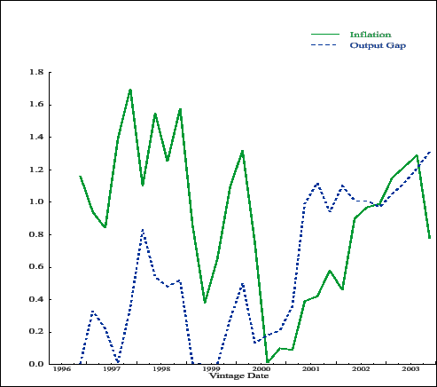
Now let us look at Figure 3.1, which shows the 5-year employment sacrifice ratio; that is, the cost in terms of cumulative annualized forgone employment, that a one-percentage-point reduction in the inflation rate would entail after five years.²¹.

**Figure 3.1:** Sacrifice ratio by vintage

When computed over a reasonably lengthy horizon such as this one, the sacrifice ratio is essentially a measure of slope of the Phillips curve. Let us focus on the red dashed line first. It shows that for the November 2003 model, the sacrifice ratio is essentially constant over time. So if the model group was asked to assess the sacrifice ratio, or what the sacrifice ratio would have been in, say, February 1997, the answer based on the November 2003 model would be the same: about 4-1/4, meaning that it would take that many percentage-point-years of unemployment to bring down inflation by one percentage point. Now, however, look at the black solid line. Since each point on the line represents a different model, and the last point on the far right of the line is the November 2003 model, the red dashed line and the black solid line must meet at the right-hand side in this and all other figures in this section. But notice how much the real-time sacrifice ratio has changed over the 8-year period of study. Had the model builders been asked in February 1997 what the sacrifice ratio was, the answer based on the February 1997 model would have been about 2-1/4, or approximately half the November 2003 answer. The black line undulates a bit, but cutting through the wiggles, there is a general upward creep over time, and a fairly discrete jump in the sacrifice ratio in late 2001.²²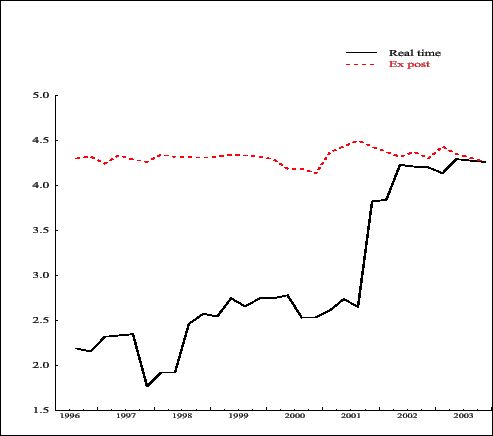

The climb in the model sacrifice ratio is striking, particularly as it was incurred over such a short period of time among model vintages with substantial overlap in their estimation periods. One might be forgiven for thinking that this phenomenon is idiosyncratic to the model under study. On this, two facts should be noted. First, even if it were idiosyncratic such a reaction misses the point. The point here is that this is the principal model that was used by the Fed staff and it was constructed with all due diligence to address the sort of questions asked here. Second, other work shows that this result is not a fluke.²³ The history of the FRB/US model supports the belief that the slope of the Phillips curve lessened, much like Atkeson and Ohanian (2001). At the same time, as we have already noted the model builders did incorporate shifts in the NAIRU (and in potential output), but found that leaning exclusively on this one story for macroeconomic dynamics in the late 1990s was insufficient. Thus, the revealed view of the model builders contrasts with idea advanced by Staiger, Stock and Watson (2001), among others, that changes in the Phillips curve are best accounted for entirely by shifts in the NAIRU.

Figure 3.2 shows the funds-rate multiplier; that is, the increase in the unemployment rate after eight quarters in response to a persistent 100-basis-point increase in the funds rate. This time, the red dashed line shows important time variation: the ex post funds rate multiplier varies with initial conditions, it is highest at a bit over 1 percentage point in late 2000, and lowest at the beginning and at the end of the period. The nonlinearity stems entirely from the specification of the model's stock market equation. In this vintage of the model, the equation is written in levels, rather than in logs, which makes the interest elasticity of aggregate demand an increasing function of the ratio of stock market wealth to total wealth. The mechanism is that an increase in the funds rate raises long-term bond rates, which in turn bring about a drop in stock market valuation operating through the arbitrage relationship between expected risk-adjusted bond and equity returns. The larger the stock market, the stronger the effect.²⁴

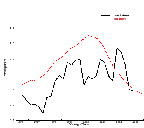
**Figure 3.2:** Funds rate multiplier by model vintage

The real-time multiplier, shown by the solid black line is harder to characterize. Two observations stand out. The first is the sheer volatility of the multiplier. In a large-scale model such as the FRB/US model, where the transmission of monetary policy operates through a number of channels, time variation in the interest elasticity of aggregate demand depends on a large variety of parameters. Second, the real-time multiplier is almost always lower than the ex post multiplier. The gap between the two is particularly marked in 2000, when the business cycle reached a peak, as did stock prices. At the time, concerns about possible stock market bubbles were rampant. One aspect of the debate between proponents and detractors of the active approach to stock market bubbles concerns the feasibility of policy prescriptions in a world of model uncertainty.²⁵ And in fact, there were three increases in the federal funds rate during 2000, totalling 100 basis points.²⁶ The considerable difference between the real-time and ex post multipliers during this period demonstrates the difficulty in carrying out historical analyses of the role of monetary policy; today's assessment of the strength of those monetary policy actions can differ substantially from what the staff thought at the time.

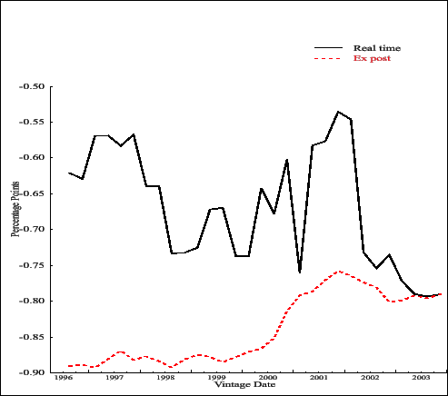
Figure 3.3 shows the government expenditure multiplier-the effect on the unemployment rate of a persistent increase in government spending of 1 percent of GDP. Noting that the sign on this multiplier is negative, one aspect of this figure is the same as the previous one: the real-time multiplier is nearly always smaller (in absolute terms) than ex post multiplier. If we take the ex post multiplier as correct, this says that policy advice based on the real-time FRB/US estimates through recent history would have routinely understated the extent to which perturbations in fiscal policy would oblige an offsetting monetary policy response. Given that the period of study involved a substantial change in the stance of fiscal policy, this is an important observation. A second aspect of the figure is the near-term reduction in the ex post multiplier, from about -0.9 in the 1990s, to about -0.75 in this decade.

**Figure 3.3:** Government expenditure multiplier by vintage

To summarize this section, real-time multipliers show substantial variation over time, and differ considerably from what one would say ex post the multipliers would be. Moreover, the discrepancies between the two multiplier concepts have often been large at critical junctures in recent economic history. It follows that real-time model uncertainty is an important problem for policy makers. The next section quantifies this point by characterizing optimal policy, and its time variation, conditional on these model vintages.

Monetary policy in real time

Optimized Taylor rules

One way to quantify the importance of model uncertainty for monetary policy is to examine how policy advice would differ depending on the model. A popular device for providing policy advice is with the prescribed paths for interest rates from simple monetary policy rules, like the rule proposed by Taylor (1993) and Henderson and McKibbin (1993). A straightforward way to do this is to compute optimized Taylor (1993) rules. Many central banks use simple rules of one sort or another in the assessment of monetary policy and for formulating policy advice. Because they react to only those variables that would be key in a wide set of models, simple rules often claimed to be robust to model misspecification. In addition, Giannone et al. (2005) show that the good fit of simple two-argument Taylor-type rules can be attributed to the small number of fundamental factors driving the U.S. economy; that is, the two arguments that appear in Taylor rules encompass all that one needs to know to summarize monetary policy in history. Thus, optimized Taylor rules would appear to be an ideal vehicle for study

Formally, a Taylor rule is optimized by choosing the parameters of the rule, $\Phi=\left\{ \alpha_{Y},\alpha_{\Pi}\right\}$ to minimize a loss function subject to a given model, $x=f(\cdot),$ and a given set of stochastic shocks, $\Sigma$ :

$LaTex Encoded Math: \displaystyle \underset{\langle\Phi\rangle}{MIN}\;% {LaTex Encoded Math: \displaystyle\sum\limits_{i=0}^{T}} \beta^{i}\left[ \left( \pi_{t+i}-\pi_{t+i}^{\ast}\right) ^{2}+\lambda _{Y}\left( u_{t+i}-u_{t+i}^{\ast}\right) ^{2}+\lambda_{\Delta R}(\Delta r_{t+i})^{2}\right]$

(2)

subject to:

$LaTex Encoded Math: \displaystyle x_{t}=f(x_{t},\ldots x_{t-j},z_{t},\ldots z_{t-k},r_{t},\ldots r_{t-m}% )+v_{t}\hspace{1in}j,k,m>0$

(3)

and

$LaTex Encoded Math: \displaystyle r=rr_{t}^{\ast}+\widetilde{\pi}+\alpha_{Y}(y_{t}-y_{t}^{\ast})+\alpha_{\Pi }(\widetilde{\pi}_{t}-\pi_{t}^{\ast})$

(4)

and

$LaTex Encoded Math: \displaystyle \Sigma_{u}=v^{\prime}v$

(5)

where is a vector of endogenous variables, and a vector of exogenous variables, both in logs, except for those variables measured in rates, $\pi$ is the inflation rate, $\widetilde{\pi}=\Sigma_{i=0}^{3}\pi_{t-i}/4$ is the four-quarter moving average of inflation, $\pi^{\ast}$ is the target rate of inflation, is (the log of) output; $y^{\ast}$ is potential output, is the civilian unemployment rate, $u^{\ast}$ is the natural rate of unemployment, and is the federal funds rate. Trivially, it is true that: $\pi,\pi^{\ast},u,u^{\ast},y^{\ast},\Delta r\in x.$ ²⁷ In principle, the loss function, (2), could have been derived as the quadratic approximation to the true social welfare function for the FRB/US model. However, it is technically infeasible for a model the size of FRB/US. That said, with the possible exception of the term penalizing the change in the federal funds rate, the arguments to (2) are standard. The penalty on the change in the funds rate may be thought of as representing either a hedge against model uncertainty in order to reduce the likelihood of the fed funds rate entering ranges beyond those for which the model was estimated, or as a pure preference of the Committee. Whatever the reason for its presence, the literature confirms that some penalty is needed to explain the historical persistence of monetary policy; see, e.g., Sack and Wieland (2000) and Rudebusch (2001).

The optimal coefficients of a given rule are a function of the model's stochastic shocks, as equation (5) indicates.²⁸ The optimized coefficient on the output gap, for example, represents not only the fact that unemployment-rate stabilization--and hence, indirectly, output-gap stabilization--is an objective of monetary policy, but also that in economies where demand shocks play a significant role, the output gap will statistically lead changes in inflation in the data; so the output gap will appear because of its role in forecasting future inflation. However, if the shocks for which the rule is optimized turn out not to be representative of those that the economy will ultimately bear, performance will suffer. As we shall see, this dependence will turn out to be significant for our results.²⁹

Solving a problem like this is easily done for linear models. However FRB/US is a non-linear model. We therefore compute the optimized rule by stochastic simulation. Specifically, each vintage of the model is subjected to bootstrapped shocks from its stochastic shock archive. Historical shocks from the estimation period of the key behavioral equations are drawn.³⁰ In all, 400 draws of 80 periods each are used for each vintage to evaluate candidate parameterizations, with a simplex method used to determine the search direction. The target rate of inflation is taken to be two percent as measured by the annualized rate of change of the personal consumption expenditure price index.³¹

This is obviously a very computationally intensive exercise and so we are limited in the range of preferences we can investigate. Accordingly, we discuss only results for one set of preferences: equal weights on output, inflation and the change in the federal funds rate in the loss function. The choice is arbitrary but does have the virtue of matching the preferences that have been used in policy optimization experiments carried out for the FOMC; see Svensson and Tetlow (2005).

The results of this exercise can be summarized graphically. In Figure 4.1, the green solid line is the optimized coefficient on inflation, $\alpha_{\Pi}$ , while the blue dashed line is feedback coefficient on the output gap, $\alpha_{Y}$ . The response to inflation is universally low, never reaching the 0.5 of the traditional Taylor (1993) rule.³² By and large, there is relatively little time variation in the inflation response coefficient. The output gap coefficient is another story. It too starts out low with the first vintage in July 1996 at about 0.2, but then rises almost steadily thereafter, reaching a peak of nearly 1 with the last vintage in November 2003. There is also a sharp jump in the gap coefficient over the first two quarters of 2001. One might be tempted to think that this is related to the jump in the sacrifice ratio, shown in Figure 3.1. In fact, the increase in the optimized gap coefficient precedes the jump in the sacrifice ratio.

**Figure 4.1:** Optimized Taylor rule coefficients by model vintage

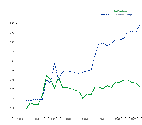
The increase in the gap coefficient coincided with the inclusion of a new investment block in the model, which in conjunction with changes to the supply block, tightened the relationship between supply-side disturbances and subsequent effects on aggregate demand, particularly over the longer term.³³ The new investment block, in turn, was driven by two factors: the addition by the Bureau of Economic Analysis a year earlier of software in the definition of equipment spending and the capital stock, and associated new appreciation on the part of the staff, of the importance of the ongoing productivity and investment boom. In any case, while the upward jump in the gap coefficient stands out, it bears recognizing that the rise in the gap coefficient was a continual process. Further discussion of some of the forces behind model changes can be found in the appendix.

Before leaving this subsection it is worth noting that similar results were obtained for Taylor rules that are extended to allow for a lagged endogenous variable as a third optimized coefficient In particular, the coefficient on the lagged fed funds rate was about 0.2 regardless of the vintage, and the coefficients on inflation and the output gap were slightly lower than in Figure 4.1, about enough to result in the same long-run elasticity.³⁴

Ex post optimal policies..." class="sectiontext">

Ex post optimal policies

We have tried to emphasize the four ingredients of model uncertainty in the real-time context: the model itself, the baseline, the policy rule, and the stochastic shocks. We also noted that these ingredients are jointly determined; in particular, Figure 4.1 showed rule coefficients that were optimal given the shocks as measured by each vintage's bootstrapped residuals. But these shocks are themselves, conditional on model design and specification decisions that were taken by the model builders. So uncertainty about the shocks one might face is also an issue, and indeed the ex post assessment of these shocks can be a driver of model respecifications. At the same time, as much as model properties and optimal policies have changed, the performance of the U.S. economy during this period was remarkably good. Four-quarter PCE inflation averaged 1-3/4 percent from 1996:Q3 to 2003:Q4 while the unemployment rate averaged 4.9 percent, according to the latest data. In this subsection, we investigate the role of the shock sets in the determination of the results in Figure 4.1. In doing so, we also (indirectly) explore one possible reason for the extraordinarily good performance of the U.S. economy during this period, namely that the FOMC may have understood the shocks as they occurred in real-time better than the model could have.

To do this, we reconsider the optimized Taylor rules of Figure 4.1, but assume this time that the Fed knows in advance the precise sequence of shocks as they occurred. So whereas the coefficients in Figure 4.1 were chosen to minimize the loss function, (2), over bootstrapped draws of the residuals, here we use just the one sequence of draws that was actually experienced. In this way, Figure 4.1 can be thought of as the ex ante optimal coefficients, so called because those coefficients are optimal given that the Fed does not know the precise sequence of shocks, and here we will look at ex post optimal coefficients.

Obviously, the idea of an ex post optimal rule is an artificial concept. It assumes information that no one could have. Moreover, if one did have such information (and knew the model with certainty as well), it would not be reasonable to restrict oneself to a simple rule like the Taylor rule. Instead, one would choose precise values of the funds rate, period by period, to minimize the loss function. Our goal here is diagnostic, not prescriptive. We are attempting to illustrate and later quantify the benefits of better real-time information. Later on, we shall look at the other side of the coin by examining the costs of the hubris of believing too much.

Before we look at the results, it is worth noting that since the ex post optimal rules are conditional on just a single "draw" of shocks, they will tend to be sensitive to relatively small changes in specification or shocks and will vary a great deal from vintage to vintage. For that reason, our comparisons with the ex ante optimal rules will be broad brush.

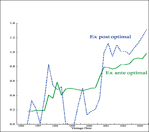
The results are shown in Figure 4.2 which can be compared with those in Figure 4.1. It is worthwhile to divide the results into two parts, demarcated by vintage: the 1990s and the new century. Volatility aside, in the 1990s the ex post optimal output-gap coefficients are mostly lower, and the inflation coefficients are mostly higher, than their ex ante counterparts. Smoothing through the wiggles, the ex post policy prescription for the late 1990s is almost one of pure inflation targeting; that is, without feedback on the output gap. We already emphasized that the late 1990s was a period dominated by persistent productivity shocks. One effect of a spate of productivity shocks, more persistent and larger than in the historical data, is to confound the usual lead-lag relationship between output fluctuations and movements in inflation, because productivity affects unit labor costs and then inflation without the necessity of changing the output gap. In these circumstances, stabilizing output becomes a less complementary device to the goal of controlling inflation than otherwise would be the case. The appropriate policy response in this instance is to focus more directly on controlling inflation and de-emphasize output stabilization. This prescription echoes that of Orphanides (2001), but operates through a different channel. Whereas Orphanides (2001) was interested in the effect of mismeasurement of the output gap, we emphasize uncertainty in stochastic shocks.

**Figure 4.2:** Ex post optimal Taylor rule coefficients by vintage

The situation in the new century is quite different. By this time, the high-tech bubble had burst and the stock market swooned-both traditional demand-side phenomena-and so the ex ante and ex post optimal coefficients look quite similar. The ex post shocks were representative of the "normal" pattern of shocks.

Also of interest given the recent literature on the subject is the response to the output gap. Figure 4.3 shows the real-time output gap coefficients for the ex ante optimal coefficients (the green solid line) and the ex post optimal (the blue dashed line). In broad terms, the two lines share some features. Both are low (on average) in the early period; both climb steeply at the turn of the century, and both continue to climb thereafter, albeit more slowly. But there are interesting differences as well, with 1999 being a particularly noteworthy period. This was a period where critics of the Fed argued that policy was too easy. The context was the three 25-basis-point cuts in the funds rate undertaken in 1998 in response to the Asia crisis and the Russian debt default. At the time, a sharp increase in investor perceptions of risk coupled with deterioration in global financial conditions raised fears of an imminent global credit crunch, concerns that played an important role in Fed decision making. By 1999, however, these factors had abated and so the FOMC starting "taking back" the previous decreases. To some, including Cecchetti et al. (2000) the easier stance undertaken in late 1998 and into 1999 exacerbated the speculative stock market boom of that time and may have amplified the ensuing recession. The ex post optimal feedback on the output gap, shown by the blue dashed line, was volatile. For the 1999 models, and given the particular shocks over the period shown in the picture, the optimal response to the gap was zero; but within months, it rose to about 0.4. In contrast, the ex ante optimal coefficients were essentially unchanged over the same period, as were the more important multipliers, which indicates that changes in the shocks were critical. Given that the shock sets in 1999 and 2000 overlap, this is a noteworthy change. To us, the important point to take from this is not the proper stance of policy at that point in history, but rather that it is so dependent on seemingly small changes. Our analysis also hints at some advantages of discretion: the willingness to respond to the specific shocks of the day-if one is able to discern them. We shall have more to say about this a bit later.

**Figure 4.3:** Comparison of output gap coefficients

Performance

To this point, we have compared model properties and the policies that those properties prescribe but have had nothing directly to say about performance. This section fills this void.

In the first subsection, we investigate how useful prior information about the sequence of shocks might be for policy and hence welfare. Specifically, we conduct counterfactual experiments on the single sequence of shocks immediately preceding each model vintage. Thus, this subsection is the performance counterpart to the design subsection of optimal ex post policies. It tells us the benefit of being right about the shock sequence underlying the ex post optimal policy. Then in subsection 5.2 , we consider the performance, on average of the model economies under stochastic simulation. The exercise in subsection 5.2 is a counterpart to the ex ante optimized policy rules in Figure 4.1. Among other things, it will tell us about the cost of being wrong in our beliefs about knowledge of the shocks.

Performance in retrospect: counterfactual experiments

If the ex post optimal rule really would have been optimal for each vintage of the model-conditional, of course, on that model-how much better would it have been than, say, the ex ante optimal rule? In other words, how valuable is that kind of information for the design of policy? We answer this question with a counterfactual simulation on selected model vintages. To facilitate comparison with the next subsection and still keep the size of the problem manageable, we restrict our attention to just two of our 30 model vintages, the February 1997 and the November 2003 vintages. These were chosen because they were far apart in time, thereby reflecting as different views of the world as this environment allows, and because their properties are the most different of any in the set. In particular, the February 1997 model has the lowest sacrifice ratio of all vintages considered, and the November 2003 model has the highest. It follows that these two models should more-or-less encompass the results of other vintages.

The details of our simulation are straightforward: each simulation is initialized with the conditions as of 20 years and two quarters before the vintage itself, as measured by that model vintage and ends two quarters before the vintage date. The Fed controls the funds rate with the policy rule in question. The model is subjected to those shocks that the economy bore over the period, as measured by the relevant model vintage. The loss in each instance is measured using the same loss function as in the optimization exercises, equation (2) and, as before, the target rate of inflation is set to two percent.³⁵ The losses are then normalized such that the historical path represents a loss of unity. All other losses can be interpreted in terms of percentage deviations from the baseline loss.

The results are shown in Table 2 below. Let us focus for the time being on the left-hand panel with the results for the February 1997 model. To aid in the interpretation of the results, the policy rule's coefficients are shown, where applicable. According to the model, the ex post optimal policy would have been superior to the historical policy. This is perhaps not all that surprising, since the ex post optimal policy has the benefit of "seeing" the shocks before they occur, although this advantage is mitigated by the constraint-not faced by the Fed-that the ex post optimal policy responds only to the output gap and the inflation rate. For this vintage, knowing the shocks turns out to be very useful indeed: the ex post policy does better-almost twice as well-as the historical policy.³⁶ However, the traditional Taylor rule also outperforms the historical policy. By contrast, the ex ante optimal policy does a fair amount worse. What both the Taylor rule and the ex post optimal policy share is stronger responses in general, and to inflation in particular, than the ex ante optimal policy. Evidently, the average sequence of shocks that conditions the ex ante optimal policy was less inflationary than the actual sequence.

Table 2: Normalized model performance in counterfactual simulation $^{\ast}$
	February 1997 vintage $\alpha_{\pi}$	February 1997 vintage $\alpha_{y}$	February 1997 vintage	November 2003 vintage $\alpha_{\pi}$	November 2003 vintage $\alpha_{y}$	November 2003 vintage
Historical policy	-	-	1	-	-	1
Ex post optimal	0.94	0.33	0.56	0.78	1.31	2.25
Ex ante optimal	0.18	0.25	1.80	0.30	1.07	4.17
Taylor rule	0.50	0.50	0.74	0.50	0.50	10.79
* Selected rules and model vintages. Using the estimated shocks over 20 years.

The right-hand panel shows the results for the November 2003 vintage of the model. Here the results are much different, and surprising. The historical policy is substantially better than any of the alternative candidates. The fact that knowledge of the shocks is an insufficient advantage to design an effective Taylor rule suggests that responding to just two variables is not enough for the shocks borne during this period. If the best two coefficients of the ex post optimal policy were less than ideal, the basic Taylor rule and the ex ante policy should do worse, and indeed they do: much worse. The lower the feedback on the output gap in these scenarios, the poorer the performance. With a bit of reflection, the reasons for this should not be surprising: the shocks during this period included shocks to the growth rate of potential output, as outlined in Figure 2.2 above. Such shocks manifest themselves in more variables than just the output gap and inflation. Indeed, the short-run impact of an increase in productivity is to reduce inflation and raise output, leading to offsetting effects on policy. However as time goes by, the higher growth rate of productivity raises the desired capital stock thereby increasing the equilibrium real interest rate. The Taylor rule and its cousins are ill designed to handle such phenomena.

Performance on average: stochastic simulations

Another way that we can assess candidate policies is by conducting stochastic simulations of the various model vintages under the control of the candidate rules and evaluating the loss function. We do this here. We subject both of these models to same set of stochastic shocks as in the ex ante optimization exercise. Under these circumstances, the ex ante optimal rule must perform the best. Accordingly, in this case, we normalize the loss under the ex ante optimal policy to unity. The results are shown in Table 3.

Table 3: Normalized model performance under stochastic simulation $^{\ast}$
	February 1997 vintage $\alpha_{\pi}$	February 1997 vintage $\alpha_{y}$	February 1997 vintage	November 2003 vintage $\alpha_{\pi}$	November 2003 vintage $\alpha_{y}$	November 2003 vintage
Ex ante optimal	0.18	0.25	1	0.30	1.07	1
Ex post optimal	0.94	0.33	1.76	0.78	1.31	4.19
Taylor rule	0.50	0.50	1.33	0.50	0.50	1.49
* Selected rules and model vintages. 400 draws of 80 periods each.

For the moment, let us focus on the left-hand panel, with the results for the February 1997 model; once again, we show the coefficients of the candidate rules for easy reference. The ex ante optimal coefficients are both low, at about 0.2. The ex post optimal coefficients are higher, particularly for inflation. However, the table shows that applying the policy that was optimal for the particular sequence of shocks to the average sequence, selected from the same set of shocks, would have been somewhat injurious to policy performance, with a loss that is 76 percent higher. The Taylor rule prescribes stronger feedback on output but weaker feedback on inflation, than the ex ante optimal policy. The fact that the loss under the Taylor rule is approximately midway between that of the ex ante and ex post rules suggests that it is the response to inflation that is the key to performance for this model vintage and the corresponding shock set. Still, in broad terms, none of the rules considered here performs too badly for this vintage.

The results for the November 2003 vintage, shown in the right-hand panel, are in some ways more interesting. Recall that in Table 2 we showed that the ex post optimal rule performed approximately twice as well as the ex ante optimal rule for the particular sequence of shocks studied. Here it is shown that this same ex post optimal rule-that is optimal for the specific shocks in the particular order of the period immediately before the vintage-performs very poorly for the same shocks on average. The reasons are clear from our prior examinations. The period ending in mid-2003 contained a number of important, correlated shocks; namely, the productivity boom and the stock market boom. The episodic nature of these disturbances makes them special. With knowledge of these shocks including the order of their arrival, a policy-even a policy constrained to respond to just two objects, inflation and the output gap-can be devised to do a reasonable job. But with randomization over these shocks, so that one knows their nature but not the specific order, the best policy is very different. This tells us is about the cost of hubris: a policy maker that thinks he knows a lot about the economy and acts on that belief, may pay a substantial price if the world turns out to be different than he expected. This impression is amplified by the Taylor rule which show performances that, while inferior to the ex ante optimal rule-as they must be-are not too bad.

One might wonder why the November 2003 model is so much more sensitive to policy settings than the February 1997 model. Earlier, we noted that performance in general is jointly determined by initial conditions (that is, the baseline), the stochastic shocks, the model and the policy rule. All of these factors are in play in these results. However, as we indicated in the previous subsection, the nature of the shocks is an important factor. The shocks for the February 1997 model come from the relatively placid period of the late 1960s to the mid-1990s, whereas the shocks to the November 2003 model contain the disturbances from the mid-1990s. We tested the importance of these shocks by repeating the experiment in this subsection using the November 2003 but restricting the shocks to the same range used for the February 1997 vintage. Performance was markedly better regardless of the policy rule. Moreover, there was less variation in performance across policy rule specifications. Since, however, the stochastic shocks come from the same data that render the model respecifications, this just emphasizes the importance of model uncertainty in general, and designing monetary policy to respond to seemingly unusual events in particular.

Discussion

In two important papers Levin et al. (1999, 2003) layout a case for judiciously parameterized simple rules as hedges against model uncertainty. In particular, they identify persistence in policy setting-a Taylor rule with a lagged fed funds rate term bearing a coefficient of unity-as being the key for robustness. At the end of subsection 4.1, we noted that none of our vintages favored a large coefficient on the lagged fed funds rate. This is surprising and particularly so since one of the models that Levin et al. (1999, 2003) used in their rival models analysis was a version of the FRB/US model. What explains the apparent contradiction? The answer is rational expectations. All of the four models that they used were linear rational expectations models where future output gaps are a key determinant of inflation. An implication of this is that missettings of the current-period funds rate have few implications for overall economic performance so long as private agents believe the policy rule guarantees a unique stable rational expectations equilibrium. ³⁷

The VAR-based expectations models used in this paper are not so forgiving. Policy errors today imply a train of events in the future that must be countered with future policy settings. The self-correcting properties in rational expectations models of agents' beliefs are not operational. We would argue that given that the premise of the literature; that is, that policy makers do not understand the model they are attempting to stabilize, the efficacy of maintaining the rational expectations assumption for private agents is open to question.

Concluding remarks

This paper has provided the first examination of real-time model uncertainty, and has done so using the archive of vintages of the FRB/US model of the macro economy since the model's inception as the Board of Governor's macroeconometric model in 1996. We examined how the model properties have changed over time and how the optimal policies for those vintages have changed alongside.

We found that the time variation in model properties is surprisingly substantial. Surprising because the period under study, at eight years, is short; substantial because the differences in model properties over time imply large differences in optimized policy coefficients.

We also compared different policies by model vintage, doing so in two different ways. In one rendition, we compared policies conditional on bootstrapped model residuals; in the other, we conducted counterfactual simulations examining performance over approximately the same period where the model vintage was estimated. Besides finding that our optimized rules differ by vintage, we also found that plausible alternatives to the optimized policy result in significant incremental losses.

Our results suggest that policy makers and researchers should not be sanguine about simple policy rules. The kind of rules promulgated by Levin et al. (1999) do not work very well in these models, the models used by the Fed staff to help inform FOMC members in their policy deliberations.

We also found that knowledge, in real time, of the disturbances the economy is bearing can, under some circumstances, be critical for good policy. In the late 1990s, a time where it is generally agreed that policy was very good, there was no Taylor rule parameterization that performed particularly well. The subject warrants further study, the findings to date point in the direction of discretionary policy with considerable attention to discerning the nature of shocks in real time as an alternative, or complement, to the use of policy rules as guides for policy.

Bibliography

Anderson, Richard G and Kevin L. Kliesen (2005)

"Productivity measurement and monetary policymaking during the 1990s" Federal Reserve Bank of St. Louis working paper no. 2005-067A (October).

Atkeson, Andrew and Lee E. Ohanian (2001)

"Are Phillips Curves Useful for Forecasting?" Federal Reserve Bank of Minneapolis Quarterly Review,25(1): 2-11.

Bernanke, Ben S., and Mark Gertler (1999)

"Monetary Policy and Asset Price Volatility" in New Challenges for Monetary Policy (Kansas City: Federal Reserve Bank of Kansas City): 77-1229

Bernanke, Ben S. and Mark Gertler (2001)

"Should Central Banks Respond to Movements in Asset Prices?" American Economic Review,91: 253-257.

Brainard, William (1967)

"Uncertainty and the Effectiveness of Monetary Policy" American Economic Review57: 411-425.

Brayton, Flint and Peter Tinsley (eds.) (1996)

"A Guide to FRB/US - a Macroeconomic Model of the United States" Finance and Economics Discussion Series paper no. 1996-42, Board of Governors of the Federal Reserve System, 1996.

Brayton, Flint, Eileen Mauskopf, David L. Reifschneider, Peter Tinsley, and John C. Williams, J.C. (1997) "The Role of Expectations in the FRB/US Macroeconomic Model" Federal Reserve Bulletin: 227-245.

Brayton, Flint , Andrew Levin, Ralph Tryon and John C. Williams (1997)

"The Evolution of Macro Models at the Federal Reserve Board" Carnegie-Rochester Conference Series on Public Policy,47: 227-245.

Cecchetti, Stephen, Hans Genberg, John Lipsky and Sushil Wadhwani (2000)

Asset Prices and Central Bank Policy The Geneva Report on the World Economy, vol. 2 (London: Center for Economic Policy Research).

Christiano, Lawrence, Martin Eichenbaum and Charles Evans (2005)

"Nominal Rigidities and the Dynamic Effects of a Shock to Monetary Policy" Journal of Political Economy,113: 1-45.

Christiano, Lawrence and Christopher Gust (1999)

"Comment" in J. B. Taylor (ed.) Monetary Policy Rules (Chicago: University of Chicago Press): 299-318.

Cogley, Timothy, and Thomas J.Sargent (2004)

"The Conquest of U.S. Inflation: Learning and Robustness to Model Uncertainty" unpublished manuscript, University of California at Davis and New York University (October).

Croushore, Dean and Thomas Stark (2001)

"A Real-time Data Set for Macroeconomists" Journal of Econometrics,105: 111-130.

Giannoni, Marc .P (2002)

"Does Model Uncertainty Justify Caution?: robust optimal monetary policy in a forward-looking model" Macroeconomic Dynamics,6: 111-144.

Giannone, Dominco, Lucrecia Reichlin and Luca Sala (2005)

"Monetary Policy in Real Time" CEPR working paper no. 4981.

Hansen, Lars.P and Thomas J.Sargent (2005)

Robustness (Princeton: Princeton University Press) forthcoming.

Dale W. Henderson and Warwick J. McKibbin (1993)

"A Comparison of Some Basic Monetary Policy Regimes for Open Economies: implications of different degrees of instrument adjustment and wage persistence" Carnegie-Rochester Conference Series on Public Policy: 221-317.

Kozicki, Sharon. and Peter Tinsley (2001)

"Shifting Endpoints in the Term Structure of Interest Rates" Journal of Monetary Economics,43: 613-652.

Kreps, David (1998)

"Anticipated Utility and Dynamic Choice" in Frontiers of Research in Economic Theory: The Nancy L. Schwartz Memorial Lectures (Cambridge: Cambridge University Press).

Levin, Andrew and John C.Williams (2003)

"Robust Monetary Policy with Competing Reference Models" Journal of Monetary Economics,50: 945-975.

Levin, Andrew, Volker Wieland and John C.Williams (1999)

"Monetary Policy Rules under Model Uncertainty" in J.B. Taylor (ed.) Monetary Policy Rules (Chicago: University of Chicago Press): 263-299

Levin, Andrew, Volker Wieland and John C.Williams (2003)

"The Performance of Forecast-based Monetary Policy Rules under Model Uncertainty" American Economic Review,93: 622-645.

McCallum, Bennett (1988)

"Robustness Properties of a Rule for Monetary Policy" Carnegie-Rochester Conference Series on Public Policy,39: 173-204.

Oliner, Stephen. and Daniel Sichel (1994)

"Computers and output growth revisited: how big is the puzzle?" Brookings Papers on Economic Activity,2: 273-317.

Oliner, Stephen. and Daniel Sichel (2002)

"The Resurgence of Growth in the Late 1990s: is information technology the story?" Journal of Economic Perspectives,14: 3-32.

Onatski, Alexei (2003)

"Robust Monetary Policy under Model Uncertainty: incorporating rational expectations" unpublished manuscript, Columbia University, 2003.

Onatski, Alexei and Noah Williams (2003)

"Modeling Model Uncertainty" Journal of the European Economic Association,1: 1087-1122.

Orphanides, Athanasios (2001).

" Monetary Policy Based on Real-time Data" American Economic Review,91: 964-985.

Orphanides, Athanasios, Richard Porter, David Reifschneider, Robert Tetlow and Frederico Finan (2000)

"Errors in the Measurement of the Output Gap and the Design of Monetary Policy" Journal of Economics and Business,52: 117-141.

Reifschneider, David L., Robert J.Tetlow and John C. Williams (1999)

"Aggregate Disturbances, Monetary Policy and the Macroeconomy: the FRB/US Perspective" Federal Reserve Bulletin (January): 1-19

Roberts, John M. (2004)

"Monetary Policy and Inflation Dynamics" Finance and Economics Discussion Series paper no. 2004-62, Board of Governors of the Federal Reserve System.

Romer, Christina and David Romer (2002)

"The Evolution of Economic Understanding and Postwar Stabilization Policy" in Rethinking Stabilization Policy (Kansas City: Federal Reserve Bank of Kansas City): 11-78.

Rudebusch, Glenn (2001)

"Is the Fed Too Timid?: monetary policy in an uncertain world" Review of Economics and Statistics,83: 203-217.

Sack, Brian and Volker Wieland (2000)

"Interest-rate Smoothing and Optimal Monetary Policy: a review of recent empirical evidence" Journal of Economics and Business,52: 205-228.

Sargent, Thomas; Noah Williams and Tao Zha (2005)

"Shocks and Government Beliefs: the rise and fall of American Inflation" forthcoming in American Economic Review.

Sims, Christopher and Tao Zha. "Were There Regime Shifts in U.S. Monetary Policy?" Federal Reserve Bank of Atlanta working paper no. 2004-14 (June).

S¨oderström, Ulf (2002) "Monetary Policy with Uncertain Parameters" Scandinavian Journal of Economics,54:125-145.

Staiger, Douglas; James H. Stock and Mark Watson (2001)

"Prices, Wages and the U.S. NAIRU in the 1990s" NBER working paper no. 8320 (June).

Svensson, Lars .E.O. (1999)

"Inflation Targeting as a Monetary Policy Rule" Journal of Monetary Economics,XLIII (1999), 607-654.

Svensson, Lars.E.O.(2002)

"Inflation Targeting: should it be modeled as an instrument rule or a targeting rule?" European Economic Review,46(4/5): 771-180.

Svensson, Lars.E.O. and Robert Tetlow (2005)

"Optimum Policy Projections" National Bureau of Economic Research working paper no 11392. Forthcoming in International Journal of Central Banking.

Svensson, Lars.E.O. and Michael Woodford (2003)

"Optimal Indicators for Monetary Policy" Monetary Economics,46: 229-256.

Taylor, John .B (1993)

"Discretion Versus Policy Rules in Practice" Carnegie-Rochester Conference Series on Public Policy,39: 195-214.

Tetlow, Robert (2005)

"Time variation in the U.S. sacrifice ratio in real time and ex post" unpublished manuscript in progress, Division of Research and Statistics, Board of Governors of the Federal Reserve System.

Tetlow. Robert and Peter von zur Muehlen.

"Robust Monetary Policy with Misspecified Models: does model uncertainty always call for attenuated policy?" Journal of Economic Dynamics and Control XXV (2001), 911-949.

Tulip, Peter (2005).

"Has Output Become More Predictable?: changes in Greenbook forecast accuracy" Finance and Economics Discussion Series paper no. 2005-31, Board of Governors of the Federal Reserve System.

Williams, John C.(2003)

"Simple Rules for Monetary Policy" Federal Reserve Bank of San Francisco Economic Review, pp.1-13.

A. Appendix

This appendix documents changes to the FRB/US model over the period from July 1996 to November 2003. The first section is fairly general, discussing the broad aspects of the model. In reflection of the importance of the productivity shock of the late 1990s on economic thought and on modeling at the Board of Governors, the second section focusses more narrowly on the model's supply block.

A.1 Model Changes by Vintage

Figures A1.a and A1.b-which are really one figure spread over two pages-provide a helicopter tour of the model's changes over time, along with reminders of some of the events of that era. The chart across the top shows two things: the total number of equation changes by vintage (the red bars, measured off the left-hand scale), and the total number of model equations, including identities (the blue line and the right-hand scale). Three facts immediately arise from the picture. First, there have been flurries of numerous changes in the model. Second, the number of changes has tended to decrease over time.³⁸ And third, the number of equations has increased, particularly in the period from 2000 to 2002. The fact that many model changes were undertaken early in the model's history but without adding to the size of the model while fewer changes were adopted later on that nonetheless added to the model's size suggests that early period was one of model shakedown while the latter period was one of revision. Indeed, during the period from about 1998 to 2002, the range of questions that the model was expected to address increased, and the staff's view of the economy became more complicated.

Figure A-1a : Model changes by vintage, 1996 - 1999

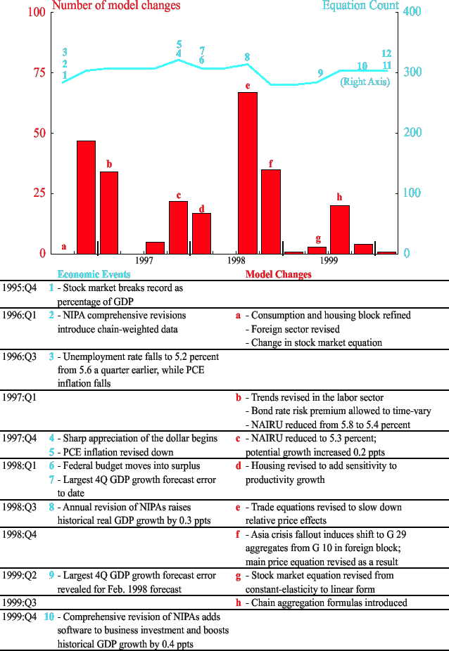
Figure A-1b : Model changes by vintage, 2000 - 2003

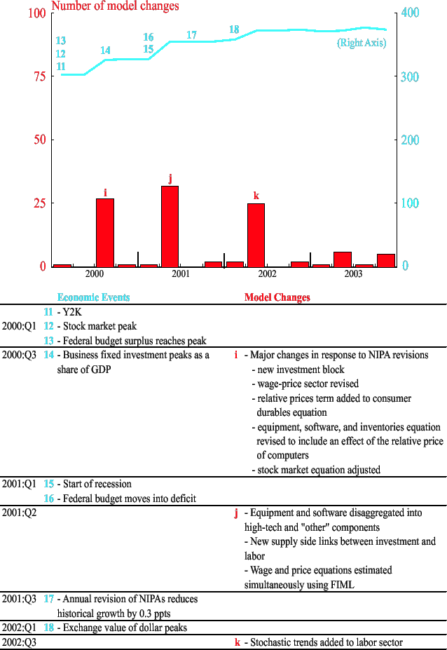
The bottom part of the two pages is a table divided into two columns. The right-hand column of each page documents some of the more important model changes incurred over the period. The entries shown are marked with a letter (in red) with a corresponding entry appearing in the appropriate place and in the same color, in the chart.

The left-hand column identifies some noteworthy economic events of the era. Some, but not all, of these events directly influenced subsequent model changes; the various NIPA revisions are stark examples of this. Other entries appearing in the left-hand column may have had a more indirect effect on model changes, or the timing of changes; some represent shocks to the model forecast that obscured, for a time, the emerging productivity boom. The Y2K phenomenon and its transitory influence on the boom in high-tech business investment in the period prior to January 1 2000 is an example. Still others appear as reminders of the economic forces that were at work during the period, which in some instances influenced the questions asked of the model. For example, the long swings in the federal budget position and the exchange value of the dollar were among the factors that changed the nature of the questions asked of the model from shorter-term forecasting issues, to medium-term policy-analysis and counterfactual-simulation issues. Analogous to the lettered entries in the right-hand column, the entries in the left-hand columns are marked by a number, with a corresponding entry appearing in the chart.

The stock market was already booming in July 1996, when the model was brought into service. By the end of the year, the model's stock market equation and the consumption and housing equations that stock market wealth affect had been changed. The most significant changes came, however, as the lasting implications of the productivity boom became prominent. In late 1999, as a part of the comprehensive revisions to the National Income and Product Accounts, software was added to the measurement of the capital stock.³⁹ Investment expenditures-particularly expenditures on information technology-boomed over the same period as did stock market valuations. By late 1999, it became clear that machinery and equipment expenditures would have to be disaggregated into high-tech and "other" because of the sharp divergence in the movements of their relative prices. The boom also engendered other questions: what is the effect of an acceleration in productivity on the equilibrium real interest rate and on the savings rate? What are the implications of persistent differences in the productivity of the high-technology and other sectors of the economy? These and other questions resulted in a reformulation of the model's supply side.

New data, new questions and new specifications interacted in complex ways. The ascent of new economic views arose in a mixture of gradual accumulation of new data, together with spurts of marked revisions to historical data. The latter came as changes in definition and concept for the NIPA data played important roles throughout this period. The revisions and conceptual changes were not exogenous events, of course, but rather reflected, in part, the changes that were going on in the economy. Table A1 below summarizes the more important statistic revisions. The table shows, first, that the revisions changed the historical "backcast" of the data is substantial ways, and second, contributed to the pro-cyclical nature of the model's revisions to potential output.

The unifying theme of the questions of the time was an reorientation toward more longer-run or lower-frequency questions than had previously been the case. The introduction of chain-weighted data in late 1996 made modeling these low-frequency trends feasible in a way that had not been the case before.⁴⁰ The point is that changes to the model were not always a reflection of the model underperforming at the tasks it was originally built to do; in many instances, it was an outcome of an expansion of the tasks to which the model was assigned.

Table A1: Major NIPA revisions and their effects, 1996-2003*
date	revision	major aspects of revision	estimated magnitude of revision
Jan. 1996	comprehensive	Adoption of chain-weighted data; new definition of government investment; new methodology for calculating capital depreciation.	Real GDP growth revised up by 0.2 percentage point, on average from 1959 to 1984, but down by 0.1 percentage point from 1987 to 1994.
July 1998	annual	New source data. Methodological changes for expenditures on cars and trucks; improved estimates on consumer services; new method of computing business inventories; some software moved from investment to business expenses.New source data.	Raised real GDP growth from 1994:Q4 to 1998:Q1 by 0.3 percentage points, mostly through higher business investment.
Oct. 1999	comprehensive	Switch to geometric weights to be consistent with earlier CPI redefinition; software included in business investment and capital stocks; new census data and 1992 benchmark input-output accounts.	Raised estimates of real GDP growth from 1987 to 1998 by an average of 0.4 percentage points.
July 2001	annual	New source data. New price index for communications equipment; conversion from SIC to NAICS industry classification system.	Reduced estimates of real GDP growth from 1998:Q1 to 2001:Q1 by 0.3 percentage points, on average.
July 2002	annual	New source data. New methodology taken on for computing wages and salaries; new price index for PCE services.	Real GDP growth revised down from 1999:Q1 to 2002:Q1 by 0.4 percentage points, on average.
* Source: based on Anderson and Kliesen (2005), Table 2.

A.2 FRB/US aggregate supply block in real time.

This section provides a summary of the evolution of the supply block of the FRB/US model. In particular, we outline the changes in the definition and behavior of potential output and its determinants over time.

As noted in the main text, changes in the model's supply side were initially driven by the lessons of the data, and in particular by a sequence of underpredictions of output with coinciding overpredictions of inflation.⁴¹ At first, the underpredictions were met with shifts in the deterministic paths of latent variables like the NAIRU and trend labor productivity. Stochastic elements of determinants of aggregate supply made their introduction in the August 1998 vintage. The first change was a relatively modest one, allowing stochastic trends in the labor force participation rate. More stochastic trends were to follow. Beginning with the May 2001 vintage, a production function accounting approach was adopted which allowed capital services to play a direct role in the evolution of potential, with stochastic trends in the average work week, the participation rate and in trend total factor productivity. The evolution from a nearly deterministic view of potential output to a stochastic view was complete. Among other things, this change in view manifests itself in more volatile measures of potential growth-and more ex post correlation between potential and actual output growth-just as the path for the August 2002 vintage shows.

The model's supply side is fairly detailed. In order to keep the exposition as short and transparent as possible, we simplify in describing certain aspects of the determinants of some variables where the simplification will not mislead the reader.⁴² Table A2 facilitates the exposition by explaining the mnemonics of the equations.


Table A2
Appendix equation mnemonics
		desired, target or equilibrium value
		output
$n^{g}$		labor productivity
		employment
		government employment
		labor force
		employment hours
		average work week
		labor quality
		civilian unemployment rate
		total factor productivity
		capital services or stock
$t\{j\}$		energy input
$d\{k\}$		wedge between payroll and establishment surveys
		time trend, commencing at date j
d{k}		shift dummy, equals zero before k and unity thereafter
mave		moving average operator

A.2.1 Aggregate supply in the July 1996 vintage

In the model's first vintage, potential output in the (adjusted) non-farm business sector, $y^{\ast},$ was the product of potential employment, $n^{\ast },$ trend labor productivity, $q^{\ast}$ , and the trend average work week, $ww^{\ast}$ , as shown by equation (A1). Equation (A2) shows that potential employment was given by the trend labor force, $lf^{\ast}$ , adjusted for the NAIRU, $u^{\ast}$ , and the trend in the wedge between the household and payroll surveys of employment, $s^{\ast}$ , less a moving average of government employment. The trend labor force is just the civilian population over the age of 16 multiplied by some time trends and shift dummies. Trend labor productivity, $q^{\ast}$ , is given by total factor productivity, $z^{\ast}$ , and a long moving average of past capital-output and energy-output ratios, multiplied by their factor shares (and divided by labor's share). Target hours, h*, was also modeled as a split time trend, as was the trend component of the wedge.

The NAIRU, $u^{\ast}$ , was set at 6 percent and trend total factor productivity, $z^{\ast}$ , was assumed to have grown exogenously at an annual rate of 2.3 percent until 1972, and have slowed to a 1.2 percent pace thereafter.

$LaTex Encoded Math: \displaystyle y^{\ast}=n^{\ast}q^{\ast}ww^{\ast}$

(A1)

$LaTex Encoded Math: \displaystyle n^{\ast}=lf^{\ast}\cdot\lbrack(1-u^{\ast})-s^{\ast}]-mave(n^{g})$

(A2)

$LaTex Encoded Math: \displaystyle lf^{\ast}=n16\cdot(b_{0}+b_{1}t47+b_{2}t901+b_{3}d90+b_{4}d94)$

(A3)

$LaTex Encoded Math: \displaystyle q^{\ast}=z^{\ast}mave(k/y)^{0.257}mave(e/y)^{0.075}$

(A4)

$LaTex Encoded Math: \displaystyle ww^{\ast}=1/\exp(a_{0}+a_{1}t47+a_{2}t801)$

(A5)

The historical record aside, the point to take from the above is that potential output was modeled as essentially deterministic. The primitives underlying the evolution of $y^{\ast}$ over time were time trends, shift dummies and slow moving averages of variables that do not fluctuate a great deal with perturbations to the data. The underlying view behind potential output at the outset of the model was a distinctly Keynesian one wherein the vast majority of fluctuations in output arose from demand-side factors.⁴³

Two other aspects of the state of the modeling world in 1996 are worth noting. First, in response to the introduction early in 1996 of chain-weighting of the National Income and Product Accounts (NIPA) data, the model section considered adding chain-weighted code to the model. However, the idea was shelved for the time being because of the volume and complexity of the necessary additional code. Second, the economic importance of computers (and associated equipment and software) were beginning to attract the attention of some of the Board staff. In particular, Oliner and Sichel [1994] studied the implications of the penetration of computers in the workplace for the measurement of capital stocks and labor productivity. At the time they regarded the stock of computers as too small to be of quantitative importance for productivity measurement. For this reason, and because the relatively new and rapidly growing high-tech sector was difficult to model, the model section opted not to split out computers (or high-tech equipment) from producers' durable equipment. Both of these decisions would be revisited, and for related reasons, as we shall see.

A.2.2 The October 1997 vintage

As the first row of Table 1 in the main text shows, by October 1997, it was apparent that the staff were about to record a large error in the forecast of GDP growth in the four quarters ending 1997:Q3: The July 1996 forecast was for growth in real GDP of 2.2 percent, while the data would eventually come in at 4.8 percent. And yet this underestimate of output growth was arising without concomitant increases in inflation as the demand-side view of the world would predict. The model builders responded by revising the model's NAIRU, raising it the 1980s to about 6.3 percent (measured on a demographically adjusted basis), and then allowing a gradual reduction over the five years from 1989 to 1993 to about 5.5 percent, or one-half percentage point below the previous estimate for this period. As before, however, $u^{\ast}$ , and other supply-side variables were extrapolated into the forecast period as exogenous trends; that is, there was no stochastic element to their revision and projection.

A.2.3 The April 1998 vintage

Instead of modeling trend labor productivity, $q^{\ast},$ as a combination of three slow-moving pieces, and allowing a residual, the model section decided to enforce the identity connecting $q^{\ast}$ and $z^{\ast}$ , eliminating the residual in the equation. Equation (A4) above still describes how trend labor productivity evolves in forecasting and simulation; in the historical data, $q^{\ast}$ however, was constructed with a kinked time trend with $z^{\ast}$ backed out. As a consequence, looked at in isolation, trend total factor productivity showed significant time variation. Mathematically, the change was of trivial importance; however, the measure of trend total factor productivity that was implied by the choice of trend labor productivity was now a variable that could be reviewed and checked for its plausibility.

A.2.4 The August 1998 vintage

The shift in the NAIRU in October 1997 aside, potential output determination remained essentially the same until the August 1998 vintage, other than some tinkering in the number and dates of breaks in trend in the $h^{\ast}$ equation. At that point, the economy was booming and more workers were being elicited to offer their employment services than the staff had previously anticipated. The model builders decided to replace the split time trend in the desired labor force, $lf^{\ast}$ , with an Hodrick-Prescott filter of the actual labor force in history and then extrapolate that trend exogenously into the forecast period.

$LaTex Encoded Math: \displaystyle lf^{\ast}=lfpr^{\ast}\cdot n16$

(A6)

$LaTex Encoded Math: \displaystyle lfpr^{\ast}=hp(lfpr)$

(A7)

The H-P filter, even though it is a two-sided filter, responds to fluctuations in the data in a way that time trends (kinked or otherwise) do not. Thus, the idea that the supply side of the economy had its (persistent) stochastic elements was introduced into the model.

At about the same time, the incipient productivity boom was raising new questions of a lower frequency (or longer-run) nature than the sorts of questions the model had originally been envisioned as answering. In particular, the model section was asking (and being asked) about the implications of a sustained increase in productivity capacity on wage determination, on stock market valuation, and on the equilibrium real interest rate. In addition, with the fiscal position of the federal government rapidly improving, questions regarding the determination of bond rates and the current account were coming to the forefront of discussion. These questions required longer-run simulations and more carefully modeled steady-state conditions than before. Approximations that had been deemed acceptable in model code for earlier vintages of the model were coming under the strain of the new demands on the model.

A.2.5 The August 1999 vintage

With the model section conducting more and more long-term simulations (simulations of, say, more than 20 years in length) the limitations of some of the approximations that had been used in place of chain-weighting in the model code were becoming apparent. What was "close enough" over an 12-quarter horizon was not close enough when approximation errors were allowed to essentially cumulate over an 80-quarter horizon. Accordingly, the section adopted chain-aggregated equations for the first time. The pertinence of this for the present discussion of the supply side of the model is that the long-duration productivity shocks, and other persistent supply shocks, that are now routinely carried out with the model could not have been done properly without chain-aggregation code.

A.2.6 The June 2000 vintage

The modeling of $ww^{\ast}$ with split time tends disappeared in favor a Hodrick-Prescott filter. Out of sample, the trend was projected exogenously. The model section's use of stochastic trends was expanding.

$LaTex Encoded Math: \displaystyle y^{\ast}=n^{\ast}q^{\ast}ww^{\ast}$

(A8)

$LaTex Encoded Math: \displaystyle ww^{\ast}=hp(ww)$

(A9)

Also around this time, Steve Oliner and Dan Sichel were completing their work, (subsequently published in 2002) on the contribution of computers and other high-tech investments to the capital stock and consequently on measured productivity. Their work would eventually allow the model group to accurately measure capital services for the first time.

A.2.7 The May 2001 vintage

May 2001 featured large-scale changes to the model's supply side. First, and most important, a full production function approach was adopted

$LaTex Encoded Math: \displaystyle y^{\ast}=(n^{\ast}ww^{\ast}nq^{\ast})^{0.700}k^{0.265}mave(e/y)^{0.0350}% z^{\ast}/(1-0.0350)$

(A10)

Second, investment in equipment and software was broken into two categories, high-tech and "other". And third, trend total factor productivity was modeled using an H-P filter, $z^{\ast}=hp(z)$ with defined as the Solow residual of the equation immediately above evaluated with instead of $y^{\ast}$ on the left-hand side. At this point, H-P filters were figuring in the construction of potential output in three places: the trend work week, the trend labor force participation rate, and trend total factor productivity.

A number of events conspired to bring about these changes (or facilitated their adoption) most of which have already been mentioned. These include the ongoing productivity boom ; the adoption of chain-aggregation model code; an acceleration in the decline in computer prices in 1999; the increase of computers and other high-tech equipment as a share of expenditures on machinery and equipment; and the BEA's comprehensive revision in December 1999 and January 2000 which added software to the definition of capital services.

The economic boom in the second half of the 1990s had made the kinked-time-trend view of trend labor productivity untenable; in the March 2001 vintage, for example, there were four breaks in trend for $q^{\ast}$ , including two as recent and as close together as 1995:Q3 and 1998:Q1. As noted above, it also changed the nature of the questions that were asked of the model, turning them more toward longer-term issues, which changed the demands on the model. Finally, the events in high-tech production and investment made the avoidance of disaggregating expenditures on machinery and equipment too costly to bear.

A.2.8 The December 2001 vintage

Concern with the two-sided nature of the H-P filter had been building for some time within the model section. If one interpreted capital put in place and labor supply as the outcome of rational, optimizing agents, then the stock of capital and the level of potential output should reflect the beliefs of firms and workers over time. It followed that "trend" variables should not use information that was not available at the time decisions are made; that is, two-sided filters should be avoided.

The first step in the section's reconsideration of this was to replace the H-P filter of the trend labor force participation rate with a (one-sided) Kalman filter estimate. The Kalman filter model allowed the change in the log of the growth rate of the labor force participation rate to be a stochastic (drift) process. The model also allowed for the influence of the unemployment rate and unidentified stationary shocks on the participation rate. With this change, a distinction was introduced between the actual growth rate of potential output, Δ y*, and the trend growth rate, g* , with the latter being interpreted as agents' beliefs about potential growth going ahead. The model had always had an expectations block, but much of the model's expectations code was concerned with short-term expectations of stationary or "gap" variables. There were, however, important exceptions to this including the expected long-run inflation rate and the expected long-run real interest rate, as well as certain levels or shares of personal income. The former two variables were based on survey and financial market data, respectively, and could reasonably be said to represent private-sector expectations. The expected income variables were ad hoc autoregressive specifications that did not allow for changes in expected growth rates. The new view of trend labor force participation was the first formal step toward broadening the pre-existing modeling convention and reflected an increased appreciation of expectations of trend growth rates. This new view would eventually have substantial effects on measures of certain latent variables such as potential output growth as a comparison of the data shown in Figure 2 of the main text makes clear. ⁴⁴

A.2.9 The March 2002 vintage

The H-P filter for the average work week is replaced by the drift component of a Kalman filter model for that variable. For the expected trend growth rate of potential, g*,a measure of the expected growth rate of trend total factor productivity is introduced. Here too, a Kalman filter is used and an I(2) drift term is extracted.

Footnotes

1. Contact address: Robert Tetlow, Federal Reserve Board, Washington, D.C. 20551. Email: [email protected]. The authors acknowledge the helpful comments of Richard Dennis, Spencer Krane, Ed Nelson, Lucrezia Reichlin, David Romer, Glenn Rudebusch, Pierre Siklos, Ellis Tallman, Daniele Terlizzese, Simon van Norden, Peter von zur Muehlen, John C. Williams, Tony Yates and seminar participants at the Federal Reserve Board, the European Central Bank, the Bank of England, the FRB-SF and the Bank of Canada. Special thanks to Dave Reifschneider for thoughtful, detailed comments and much patience. We thank Flint Brayton for helping us interpret the origins of many of the model changes, and Douglas Battenberg for help getting the FRB/US model archives in working order. Part of this research was conducted while the first author was visiting the Bank of England and the San Francisco Fed; he thanks those institutions for their hospitality. All remaining errors are ours. The views expressed in this paper are those of the authors alone and do not represent those of the Federal Reserve Board or other members of its staff. Return to Text

2. Levin et al. (1999), use four models as rivals but all were New Keynesian linear rational expectations models with wage-price (or Phillips curve) mechanisms that run off of output gaps. Williams (2003) demonstrates that linear rational expectations models are very forgiving of perturbations in policy rules in the sense that a deviation from the optimized coefficients of a Taylor-type rule does not substantially change policy outcomes provided that the model under control is still stable, a property not shared by models with little or no rationality of expectations. This, plus the similarity of the monetary policy mechanisms in the four models limits the applicability of Levin et al. [1999] to broader environments, as Levin and Williams (2003) shows. Return to Text

3. Robust control theory is also sometimes advocated; see, e.g., Hansen and Sargent (2005), Giannoni (2002), Onatski (2001) and Tetlow and von zur Muehlen (2001). In this instance, the policy maker seeks to protect against a worst-case outcome to misspecification in the neighborhood of a reference model. The difficulty in this instance is in the specifying the neighborhood. Return to Text

4. There is an extensive literature on the design of monetary policy under uncertainty. Most of it deals with data or parameter uncertainty. Techniques for handling these issues are now well known; see, e.g., Svensson and Woodford (2003) and references therein. In most instances, the optimal response is either certainty equivalence or attenuation of policy reponses relative to the certainty equivalent policy reaction. A counterexample to the usual attenuation case is Söderström (2002). Return to Text

5. There have been a number of valuable contributions to the real-time analysis of monetary policy issues. Most are associated with data and forecasting. See, in particular, the work of Croushore and Stark (2001) and a whole conference on the subject details of which can be found at http://www.phil.frb.org/econ/conf/rtdconfpapers.html An additional, deeper layer of real-time analysis considers revisions to unobservable state variables, such as potential output; on this see Orphanides et al. (2000) and Orphanides (2001). See also Giannone et al. (2005) for a sophisticated, real-time analysis of the history of FOMC behavior. Return to Text

6. More precisely we adjust potential non-farm business output where the adjustment is to exclude owner occupied housing, and to include oil imports. This makes output conformable with the model's production function which includes oil as a factor of production. Henceforth it should be understood that all references to productivity or potential output are to the concept measured in terms of adjusted non-farm business output. Return to Text

7. Defined in this way, data uncertainty does not include uncertainty in the measurement of latent variables, like potential output. The important conceptual distinction between the two is that eventually one knows what the final data series is-what "the truth" is-when dealing with data uncertainty. One never knows, even long after the fact, what the true values of latent variables are. Latent variables are more akin to parameter uncertainty than data uncertainty. On this, see Orphanides et al. (2000) and Orphanides (2001). Return to Text

8. A record such as the one in the table was not unusual during this period; the Survey of Professional Forecasters similarly underpredicted output growth. Tulip (2005) documents how the official Greenbook forecast exhibited a similar pattern of forecast errors. Return to Text

9. Some details on this evolution of thought are provided in the Appendix. Return to Text

10. Thre were methodological changes to expenditures and prices of cars and trucks; impoved estiamted of consumer expenditures on services; new methods of computing changes in business inventories; and some expenditures on software by businesses were removed from business fixed investment and reclassified as expenses. Return to Text

11. The model introduced the notion of polynomial adjustment costs, a straightforward generalization of the well-known quadratic adjustment costs, which allowed, for example, the flow of investment to be costly to adjust, and not just the capital stock. This idea, controversial at the time, has recently been adopted in the broader academic community; see e.g., Christiano, Eichenbaum and Evans (2005). Return to Text

12. That is, polynomial adjustment costs in price and volume decision rules. In financial markets, intrinsic adjustment costs were assumed to be zero. Return to Text

13. This idea has been articulated and extended in a series of papers by Kozicki and Tinsley. See, e.g., their (2001) article. Return to Text

14. More recently, the model section has added to its repertoire optimal control policy experiments conducted on a version of model with rational expectations in asset prices. Return to Text

15. Stochastic simulation and optimization of a large-scale non-linear rational expectations model is a Hurculean task. In any case, a complete set of archives of the perfect-foresight version of the model is not available. Return to Text

16. Nothing of importance is lost from the analysis by excluding every second vintage from consideration. The archives are listed by the precise date of the FOMC meeting in which the forecasts were discussed. For our purposes, we do not need to be so precise so we shall describe them by month and year. Thus, the 30 vintages we use are, in 1996: July and November; in 1997: February, May, July, and November; in 1998 through 2000: February, May, August and November; and in 2001 through 2003: January, May, August and November. Return to Text

17. Each vintage has a list of variables that are shocked using bootstrap methods for stochastic simulations. The list of shocks is a subset of the model's complete set of residuals since other residuals are treated not as shocks but rather as measurement error. The precise nature of the shocks will vary according to data construction and the period over which the shocks are drawn. Return to Text

18. The transcript of the July 2-3, 1996 FOMC meeting (p. 42) quotes then Fed Governor Janet Yellen: "The sacrifice ratio in our new FRB-US model, without credibility effects, is 2.5..." Based on this figure and other arguments, Gov. Yellen spearheaded a discussion of what long-run target rate of inflation the FOMC might wish to achieve. Yellen is now President of the Federal Reserve Bank of San Francisco. Return to Text

19. The Board staff present their analysis of recent history, the staff forecast and alternative simulations, the latter using the FRB/US model, in the Greenbook. The FOMC also receives detailed analysis of policy options in the Bluebook Alternative policy simulations are typically carried out using the FRB/US model. In addition, for the FOMC's semi-annual two-day meetings, detailed reports are often prepared by the staff and these reports frequently involve the FRB/US model. Go to http://www.federalreserve.gov/fomc/transcripts/ for transcipts of FOMC meetings as well as the presentations of the senior staff to the FOMC. See Svensson and Tetlow (2005) for a related discussion. Return to Text

20. Another way of examining the same thing would be to initiate each of the ex ante multipliers experiments at the same date in history and compare these with the black line in each figure. Such an experiment is not completely clean, however, because each model is only conformable with its own baseline database and these baselines have different conditions for every given date as Figures 2.1 through 2.4 demonstrated. Nonetheless, the results of such an exercise are available from the corresponding author on request. Return to Text

21. More precisely, the experiment is conducted by simulation, setting the target rate of inflation in a Taylor rule to one percentage point below its baseline level. The sacrifice ratio is cumulative annualized change in the unemployment rate, undiscounted, relative to baseline, divided by the change in PCE inflation after 5 years. Other rules would produce different sacrifice ratios but the same profile over time. Return to Text

22. The sizable jump in the sacrifice ratio in late 2001 is associated with a shift to estimating the models principle wage and price equations simultaneously together with other equations to represent the rest of the economy, including a Taylor rule for policy. Among other things, this allowed expectations formation in wage and price setting decisions to reflect more recent Fed behavior than the full core VAR equations that are used in the rest of the model. See the Appendix for more details. Return to Text

23. In particular, the same phenomenon occurs to varying degrees in simple single-equation Phillips curves of various specifications using both real-time and ex post data; see Tetlow (2005b). Roberts (2004) shows how greater discipline in monetary policy may have contributed to the reduction in economic volatility in the period since the Volcker disinflation. Cogley and Sargent (2004) use Bayesian techniques to estimate three Phillips curves and an aggregate supply curve simultaneously asking why the Fed did not choose an inflation stabilizing policy before the Volcker disinflation. They too find time variation in the (reduced-form) output cost of disinflation. See, as well, Sargent, Williams and Zha (2005). Return to Text

24. The levels relationship of the stock market equation means that the wealth effect of the stock market on consumption can be measured in the familiar "cents per dollar" form (of incremental stock market wealth). Return to Text

25. The "active approach" to the presence of stock market bubbles argues that monetary policy should specifically respond to bubbles. See, e.g., Cecchetti et al. (2000). The passive approach argues that bubbles should affect monetary policy only insofar as they affect the forecast for inflation and possibly output. They should not be a special object of policy. See, Bernanke and Gertler (1999, 2001). Return to Text

26. The intended federal funds rate was raised 25 basis points on February 2, 2000, to 5-3/4 percent; by a further 25 basis points on March 21, and by 50 basis points on May 16, to 6-1/2 percent. Return to Text

27. The intercept used in the model's Taylor rule, designated $rr^{\ast}$ , is a medium-term proxy for the equilibrium real interest rate. It is an endogenous variable in the model. In particular, $rr_{t}^{\ast}=(1-\gamma)rr_{t-1}^{\ast }+\gamma(rn_{t}-\pi_{t})$ where

is the federal funds rate, and $\gamma$ =0.05. As a robustness check, we experimented with adding a constant in the optimized rules in addition to $rr^{\ast}$ and found that this term was virtually zero for every model vintage. Note that relative to the classic version of the Taylor rule where $rr^{\ast}$ is fixed, this alteration biases results in favor of good performance by this class of rules. Return to Text

28. Our rules will be optimal in the class of Taylor-type rules of the form in equation (4), conditional on the stochastic shock set, (5), under anticipated utility as defined by Kreps (1996). Return to Text

29. The fact that the policy rule depends on the variance-covariance matrix of stochastic shocks means that the rule is not certainty equivalent. This is the case for two reasons. One is the non-linearity of the model. The other is the fact that the rule is a simple one: it does not include all the states of the model. Return to Text

30. The number of shocks used for stochastic simulations has varied with the vintage, and generally has grown. For the first vintage, 43 shocks were used, while for the November 2003 vintage, 75 were used. Return to Text

31. For these experiments any reasonable target will suffice since the stochastic simulations effectively randomize over initial conditions. Return to Text

32. That said, the measure of inflation differs here. In keeping with the tradition of inflation targeting countries, we use the rate of the change in the PCE price index as the inflation rate of interest. Taylor (1993) used the GDP price deflator. Return to Text

33. In essence, the linkage between a disturbance to total factor productivity and the desired capital stock in the future was clarified and strengthened so that an increase in TFP that may produce excess supply in the very short run can be expected to produce an investment-led period of excess demand later on. Return to Text

34. . This result is consistent with the finding of Rudebusch (2001) for the Rudebusch-Svensson model, but differs from that of Williams (2003) for a linearized rational expectations version of the FRB/US model. The reason is that without rational expectations, the efficacy of "promising" future settings of the funds rate through instrument smoothing is impaired. Return to Text

35. In a discussion of inflation targeting at the FOMC meeting in July 1996-the same date as our first model vintage-most members the FOMC appeared to have agreed that 2 percent would have be a reasonsable target rate of inflation. The thorny issues of settling on a particular index and the assessment of, and correction for, measurement error in price indexes remained unsettled. See http://www.federalreserve.gov/fomc/transcripts/1996/19960703Meeting.PDF, especially at pp. 63-65. Return to Text

36. That said, as we noted before, the performance comparison assumes preferences that may not match the FOMC's preferences, although they are arguably very reasonable preferences. Return to Text

37. The evidence for this is contained in Levin and Williams (2003) where it is shown that policy makers face a more difficult choice in finding a robust policy if one of the rival models is a linear rational expectations model and another is a "backward-looking" model. Cogley and Sargent (2004) point to a similar issue in their work explaining the runaway inflation of the 1970s. Return to Text

38. A "model change" is the non-trivial addition, deletion or change in specification of a "significant" model equation from the vintage immediately preceding. Re-estimation of a given equation does not count as a model change. Rewriting an equation in a mathematically equivalent way also does not count. In a fully articulated model with a large number of identities, changes in structural equations can oblige corresponding changes in a large number of associated identities. As a result, the count of model changes mounts rapidly. Return to Text

39. Prior to that time, expenditures on software were regarded as an intermediate input; they had no direct effect on GDP. Return to Text

40. In the absence of chain-weighting, trends in relative prices, like the relative price of high-tech capital goods, could not be modeled well. The inability to account for weight shifts in expenditure bundles, which was merely a nuisance over short horizons, was a substantial barrier for the analysis of longer-term phenomena. Return to Text

41. Svensson and Tetlow [2005] document the change in the Board staff's view between 1997 and 1999. Tulip [2005] summarizes the forecast record of the Board staff over this period and others. In both of these papers, it is the staff economic projection-a judgmental forecast-rather than the model forecast that is discussed but the records of the two forecasts were quite similar. Return to Text

42. For example, below we describe the describe trend labor productivity as being a geometric weighted sum of lagged capital-to-output and energy-to-output ratios. This is true, but these actual ratios are then modeled as a function of desired ratios, which in turn are a function of the ratio of output price to user cost. Return to Text

43. Perhaps more accurately it could be said that persistent supply shocks were infrequent enough that they could be disregarded as improbable, ex ante, and large enough that they could be identified in real time. Return to Text

44. This distinction is the main reason why the growth rate of potential for the August 2002 vintage shown in Figure 2 looks so much more volatile than its predecessors. The expected growth rate upon which some of the model's agents base their decisions at any given date in history was smoother. At this stage, however, with just the labor force particpation rate modeled using the Kalman filter, the distinction was not all that large. Return to Text

This version is optimized for use by screen readers. A printable pdf version is available.

Real-time Model Uncertainty in the United States: the Fed from 1996-20031