Skip to: [Printable Version (PDF)] [Bibliography] [Footnotes]

Finance and Economics Discussion Series: 2006-30 Screen Reader version*

GSEs, Mortgage Rates, and Secondary Market Activities^*

Andreas Lehnert
Board of Governors of the
Federal Reserve System
Washington, DC 20551
(202) 452-3325
[email protected]

Wayne Passmore
Board of Governors of the
Federal Reserve System
Washington, DC 20551
(202) 452-6432
[email protected]

Shane M. Sherlund
Board of Governors of the
Federal Reserve System
Washington, DC 20551
(202) 452-3589
[email protected]

This Version: September 8, 2006

We welcome all comments; please contact us directly for the latest version.

Keywords: Mortgage finance, Government-Sponsored Enterprises, Financial stability

Abstract:

Fannie Mae and Freddie Mac are government-sponsored enterprises (GSEs) that securitize mortgages and issue mortgage-backed securities (MBS). In addition, the GSEs are active participants in the secondary mortgage market on behalf of their own investment portfolios. Because these portfolios have grown quite large, portfolio purchases (in addition to MBS issuance) are often thought to be an important force in the mortgage market. Using monthly data from 1993 to 2005 we estimate a VAR model of the relationship between GSE secondary market activities and mortgage interest rate spreads. We find that GSE portfolio purchases have no significant effects on either primary or secondary mortgage rate spreads. Further, we examine GSE activities and mortgage rate spreads in the wake of the 1998 debt crisis, and find that GSE portfolio purchases did little to affect interest rates paid by new mortgage borrowers. This empirical finding is robust to alternative identification assumptions and to alternative model and variable specifications.

Journal of Economic Literature classification numbers: H81, G18, G21

1 Introduction

The housing-related government-sponsored enterprises (GSEs) Fannie Mae and Freddie Mac securitize pools of mortgages, thereby assuming their credit risk and allowing the resulting mortgage-backed securities (MBS) to trade as effectively AAA-rated securities. This process provides originators access to a liquid secondary market for their loans. Separately, the GSEs also issue corporate bonds to finance large, highly leveraged, portfolios of mortgages, often in the form of their own MBS.

The GSEs, through their portfolios, are large investors in the U.S. mortgage market. At the end of 2004, GSE-issued MBS totaled nearly $2.7 trillion, or nearly 35 percent of outstanding home mortgage debt. At the same time, GSE portfolios totaled over $1.5 trillion, or more than 20 percent of total mortgage debt. In a typical month, roughly 40 percent of newly originated mortgages are securitized by the GSEs, and about 20 percent are bought by the GSEs' portfolios.¹Given their important role in mortgage markets, one might expect the quantities purchased by the GSEs to affect the equilibrium prices in mortgage markets. Indeed, the GSEs' effect on mortgage rates has played a key role in the recent policy debates on how to reform the GSEs (Greenspan (2005b)).

Earnings from mortgages held in the GSEs' portfolios clearly benefit GSE shareholders. But these portfolios might also benefit mortgage originators and home buyers with conforming mortgages. Unusually heavy and sustained portfolio purchases might bid up the price of new mortgages, allowing originators greater profits or the opportunity to lower mortgage rates. However, the GSEs must finance such purchases by issuing corporate debt. Thus the extra demand for mortgage assets created by portfolio purchases might be largely offset by the increase in GSE corporate debt.

However, even if GSE portfolio purchases do not affect mortgage rates during normal times, the purchases might act as a stabilization mechanism during financial crises, with the GSEs acting as a buyer of last resort in the MBS market. The GSEs might then buffer mortgage originators from financial market shocks, thereby limiting the impact of shocks on mortgage rates and mortgage borrowers.

The ability of GSE portfolio purchases to affect MBS prices depends in part on whether investors view GSE-guaranteed MBS and GSE corporate debt as substitutes. Roll2003, among others, argues that foreign investors prefer holding GSE debt over GSE-guaranteed MBS because some GSE corporate bonds do not carry the prepayment risk inherent in MBS. In this view, GSE portfolio growth would stimulate lower-cost foreign capital to flow into U.S. mortgage markets. By the same argument, however, this capital would flow out of corporate and Treasury markets. Moreover, other intermediaries can construct synthetic securities based on MBS that strip out prepayment risk. Given the size and diversity of the U.S. high-quality debt market (more than $23 trillion according to the Federal Reserve's Flow of Funds Accounts), the importance of foreign investors in mortgage rate determination might be very small. Indeed, the large market for highly rated debt suggests that mortgage rates are set in worldwide capital markets and that GSE portfolios might have little influence on mortgage rates.

Investors demand lower returns on GSE corporate debt than on the debt of other comparable corporations, partly because investors perceive an implicit government guarantee on the debt. One might expect some of this implicit subsidy to flow to mortgage borrowers. Previous literature has examined several channels by which the GSEs could affect mortgage rates. By law, the GSEs cannot buy mortgages larger than the conforming loan limit (such large mortgages are known as jumbos). Several papers have estimated the difference between mortgage rates on jumbo loans and those on conforming loans. Recent estimates of this spread range from 4 to 35 basis points, while older estimates are often times even higher.² Other studies have examined the effect of the GSEs' activities on conforming mortgage rate spreads.³

In this paper we use a vector autoregression (VAR) approach and monthly data from March 1993 to December 2005 to estimate the effect of GSE secondary market activities--both gross portfolio purchases and MBS issuance--on primary and secondary mortgage rate spreads. Our main finding is that GSE portfolio purchases have essentially no short- or long-run effects on either primary or secondary mortgage rate spreads. We also find some evidence that GSE portfolio purchases tend to rise following an increase in spreads; if spreads are mean-reverting, such behavior is consistent with a profit-maximizing portfolio strategy.

Our results are subject to some obvious caveats. First, and most importantly from a policy perspective, our results are subject to the Lucas critique. We are not estimating the deep parameters of a fully specified theoretical model featuring optimizing forward-looking market participants. Thus, our estimated effects can only describe the behavior of the endogenous variable under the policy regime of the sample period. However, our results can be used to evaluate the claims of an effect over the sample period. Further, given that secondary markets for nonconforming mortgages are growing in sophistication and size, the effectiveness of GSE actions (which primarily affect conforming mortgages) seems more likely to diminish than to grow.

Second, we are limited by our data to studying the relationship among GSE actions and interest rates at a monthly frequency. If GSE actions and interacted spreads at a much higher frequency we might not find any relationships using monthly data. However, even at a monthly frequency, we do find several interesting dynamic relationships; thus, we do not believe that our results are driven by time-aggregation bias. Moreover, we show that spreads and GSE actions are not particularly correlated within a month (although GSE actions are correlated with lagged shocks to spreads). Thus, there is simply not very much causality to assign within a given month.⁴ Finally, other studies of the relationship between GSE portfolios and mortgage rates have used monthly data while none (to the best of our knowledge) have had access to higher-frequency data.

Third, and related, the classic structural VAR methodology requires the econometrician to make identifying assumptions about how the endogenous variables react to one another within the same period. The commonly used triangular ordering, for example, requires the econometrician to specify that some variables react to others only after a delay. In our model, this would require assuming that, for example, GSE portfolio purchases could react to changes in spreads within a given month but that spreads could not react to portfolio purchases (or vice versa). However, in place of the standard structural VAR identifying assumptions, we use the weaker identifying assumptions suggested by Pesarin and Shin (1998). These produce impulse response functions that are not affected by the ordering of the shocks. In our robustness tests, we show that our results are essentially unchanged under several different identifying assumptions.

Our main results are also robust to a variety of alternative specifications. In particular, we estimated the effect of GSE actions on mortgage spreads in models that use (1) nonstationary techniques, (2) alternative scaling factors and variable definitions to produce stationary series, and (3) a variety of time series identifying assumptions including the full set of triangular shock orderings.

Our paper is closest to the study of Naranjo and Toevs (2002), who estimate a long-run cointegrating relationship between GSE portfolio purchases and mortgage rate spreads. In contrast with our results, they conclude that GSE portfolio purchases lower primary mortgage rate spreads and that portfolio purchases lower primary mortgage rates more than MBS issuance. Because they used proprietary data from Fannie Mae to construct their dataset we cannot attempt to replicate their study. However, even under our closest approximation to their specification we are unable to reproduce several key findings from their study.⁵

Our paper is also similar to the study of Gonzales-Riviera (2001), who estimates a long-run cointegrating relationship between secondary market spreads and portfolio purchases using monthly data from 1994 to 1999. She concludes that wider secondary market spreads increase portfolio purchases and finds that the "error correction term in the equation for portfolio purchases is not statistically significant" and therefore "it is mainly movements in the secondary market spread that will carry out the adjustment toward equilibrium, in the very short term" (p. 33). Thus, Gonzalez-Rivera's results also cast doubt on the ability of portfolio purchases to affect spreads.⁶

The GSEs' large, highly leveraged portfolios pose risks to the taxpayer and to the financial system more broadly.⁷ Our results suggest that curbing the growth of these portfolios might not increase mortgage rates paid by new mortgage borrowers while mitigating the risks posed to taxpayers and the financial system.⁸

The remainder of the paper is organized as follows. In the next section, we introduce the VAR. The third section presents our data. Section 4 contains our results, our analysis of GSE secondary market activities on mortgage rate spreads, and an analysis of GSE activities during the financial market distress of late 1998. The next section presents various robustness checks and the final section concludes.

2 VAR and Identification

In this section we discuss the economic environment in which our data are generated and our statistical approach. Broadly speaking, we estimate a vector autoregression (VAR) model with GSE actions and mortgage rate spreads as endogenous variables. Our primary conceptual experiment is how one variable will evolve over time in reaction to a shock to a different variable, e.g., how mortgage rate spreads will change if GSE portfolio purchases suddenly increase. Following the literature, we compute impulse response functions (IRFs) to match the conceptual experiments. However, in our baseline specification, we do not use the standard (strong) identifying assumptions to construct our IRFs; instead we follow Pesarin and Shin (1998) and use weaker identifying assumptions to construct generalized impulse response functions.

2.1 Overview

Mortgage interest rate spreads are affected by investors' expectations about mortgage risks (mainly credit and prepayment risks), financial market liquidity, investors' expectations about the actions of other participants (including the GSEs), and the current level and expected trajectory of mortgage rate spreads. At the same time, the GSEs are buying mortgages for their own investment portfolios for many of these same reasons.

The theoretical connection among these variables could be quite complicated, in part because the equilibrium depends on how a small number of entities expects the others to behave. In this paper, we do not attempt to estimate the deep parameters of such a theory-based structural model.⁹ Instead, in our reduced-form approach our goal is to characterize the statistical relationship among the endogenous variables, including the potential stabilizing effects of GSE activities on mortgage rate spreads and the GSE portfolio managers' reactions to mortgage rate spreads.

Our techniques allow us to examine the short- and long-run effects of GSE portfolio purchases on mortgage rate spreads. Note that lowering mortgage rates in the short run does not require permanently lowering them, or vice-versa. The GSEs might be able to dramatically affect mortgage rate spreads in the short run, but then see these effects undone over time, leaving mortgage rate spreads unchanged in the long run. Conversely, the GSEs might not be able to affect mortgage rate spreads much in the short run, but might be able to cumulate their effects over time, producing a significant long-run effect.

An obvious shortcoming of our data is its monthly frequency. Financial market prices and traders routinely interact at a much higher frequency. Given that our data are monthly, it is difficult to ascribe causation to correlated movements between GSE activities and mortgage rate spreads. That is, if GSE portfolio purchases rose and mortgage rate spreads fell within a month, we could not say to what degree GSE business managers reacted to larger-than-expected mortgage rate spreads by increasing portfolio purchases, and to what degree larger-than-expected GSE portfolio purchases pushed down mortgage rate spreads. The standard Cholesky-style identification scheme would require choosing a priori the direction of contemporaneous causality.

In this paper, however, we use a more general identification strategy that eliminates the need to specify an a priori ordering of variables within the VAR. Pesarin and Shin (1998) (following Koop, G., M. H. Pesaran, and S. M. Potter (1996)) derive generalized impulse response functions that are invariant to the ordering of variables in the VAR. This procedure is a deviation from standard practice, so we will describe it in some detail here.

2.2 Basic Model

Formally, we arrange the endogenous variables (such as mortgage rate spreads and portfolio purchases) in each period into the vector and the exogenous variables (such as the risk-free rate and the slope of the yield curve) into the vector . We then write the structural relationship between the endogenous and exogenous variables as:

(1)	$\displaystyle \Phi_0 X_t = \Phi_1 X_{t-1} + \cdots + \Phi_p X_{t-p} + \Gamma_0 Z_t + \Gamma_1 Z_{t-1} + \cdots + \Gamma_k Z_{t-k} + \varepsilon_t.$

Here, $\Phi_j$ ( $n\times n$ ) and $\Gamma_j$ ( $n\times m$ ) denote coefficient matrixes and $\varepsilon_t$ ( $n\times 1$ ) denotes the vector of fundamental shocks to the economic system. Because these shocks are taken to be independent we assume that their variance-covariance matrix is diagonal and given by: $E\left(\varepsilon_{t}\varepsilon_{t}^{\prime}\right)= \Lambda_n$ .

In our primary specification, the vector of endogenous variables includes five variables: the secondary mortgage rate spread, the primary mortgage rate spread, implied volatility on ten-year Treasuries, gross GSE MBS issuance, and gross GSE portfolio purchases. The vector of exogenous variables includes three variables: realized mortgage delinquencies, the ten-year Treasury rate, and the Treasury yield curve slope (1 to 10 year). Each of these variables is described in more detail in the next section.

We cannot estimate the coefficients of the structural representation given by equation (1) directly. Instead, we estimate the coefficients of the reduced-form representation:

(2)	$\displaystyle X_t = A_1 X_{t-1} + \cdots + A_p X_{t-p} + B_0 Z_{t} + \cdots + B_k Z_{t-k} + u_t.$

Here

is the vector of reduced-form errors. In moving from equation (1) to equation (2) we left-multiplied both sides of equation (1) by $\Phi_0^{-1}$ . Thus the reduced-form error

will be a linear combination of the fundamental shocks $u_t=\Phi_0^{-1}\varepsilon_t$ . The errors

will, as a result, be correlated across equations so that their variance-covariance matrix generally will be non-diagonal:

$\displaystyle E\left(u_t{u_t}^{\prime}\right)= E\left(\Phi_0^{-1}\varepsilon_t {\varepsilon_t}^{\prime}{\Phi_0^{-1}}^{\prime}\right)= \Phi_0^{-1}E\left(\varepsilon_t {\varepsilon_t}^{\prime}\right){\Phi_0^{-1}}^{\prime}= \Phi_0^{-1}\Lambda_n{\Phi_0^{-1}}^{\prime}\equiv S$

Our fundamental identification problem is to produce estimates of the structural parameters from the estimated reduced-form coefficients. The reduced-form parameters will provide us with fewer coefficients than we require to pin down the structural parameters, requiring us to make additional a priori assumptions about the structural parameters. More formally, the structural equation contains the following free parameters:

$\displaystyle \underbrace{\Phi_0}_{n^2-n}\ , \underbrace{\Phi_1 \cdots \Phi_p}_{p\times n^2}\ , \underbrace{\Gamma_1 \cdots \Gamma_k}_{k\times nm}\ , \underbrace{\Lambda_n}_{n}\rightarrow n^2+pn^2+kmn\$ free parameters $\displaystyle .$

The matrix $\Phi_0$ has only

free parameters because the diagonal elements are assumed to be unity. The reduced-form estimates provide us with the following coefficient estimates:

$\displaystyle \underbrace{A_1\cdots A_p}_{p\times n^2}, \underbrace{B_0\cdots B_k}_{k\times nm}, \underbrace{S}_{(n^2+n)/2} \rightarrow pn^2 + kmn + (n^2+n)/2\$ coefficients $\displaystyle .$

Thus, the number of restrictions we have to impose in order to identify the structural parameters is the difference between the two, or

. In our baseline model, where

, we require 10 restrictions.

2.3 Standard Impulse Response Functions

In our results section we will focus on the impulse response functions implied by our estimated coefficients. The conceptual experiment is to compare the trajectories of the endogenous variables under two scenarios: in one scenario (the control) we assume that, at the end of period nothing is known about the fundamental shocks that will hit the economy in period ; in the other scenario (the experiment) we assume that at the end of period market participants become aware that next period's fundamental shock will be such that $u_t=\delta$ . We then compute the expected values of the endogenous variables in periods , , , and so on; the impulse response function will be the difference between the expectations under the experiment and under the control.

To simplify notation, assume that the structural model (1) features only one lag of the endogenous variables and no exogenous variables (other than the shocks $\varepsilon$ ). This assumption is not as restrictive as it might seem because the estimated coefficients on the exogenous and extra lagged endogenous variables in the reduced-form representation provide no net restrictions on the parameters of the structural representation.¹⁰ Thus, we rewrite equation (2) as:

(2')	$\displaystyle X_t = A_1X_{t-1} + u_t.$

We can use equation (2') to write

as the sum of the

's:

(3)	$\displaystyle X_t = u_t + A_1u_{t-1} + A_1^2u_{t-2} + A_1^3u_{t-3} + \cdots.$

Our conceptual experiment (the impulse response function) can be written as:

$\displaystyle E_{t-1}\left\{X_{t+j}\vert u_{t}=\delta\right\} - E_{t-1}\left\{X_{t+j}\right\},\ j=0,1,\ldots.$

From equation (3) we see that for each period

this difference is:

$\displaystyle E_{t-1}\bigl(X_{t+j}\vert u_{t}=\delta\bigr)-E_{t-1}\bigl(X_{t+j}\bigr) = A_1^j\delta.$

The shock to the reduced-form system $\delta$ is usually constructed to represent an innovation to one of the fundamental shocks $\varepsilon_t$ . For example, a unit innovation to the first equation in our system might be written as $\delta_{\varepsilon}=(1,\ 0,\ 0,\ 0,\ 0)^{\prime}$ . Because $u_t=\Phi_0^{-1}\varepsilon_t$ , $\delta$ would be written as: $\delta = \Phi_0^{-1}\delta_{\varepsilon}.$

Under this approach, we need an estimate of $\Phi_0$ in order to construct $\delta$ . As we discussed in the previous section, we need to impose restrictions. The usual set of restrictions is that $\Phi_0$ be lower triangular, that is, all values above the diagonal are zero. With this assumption, we can form an estimate of $\Phi_0$ and $\Lambda_n$ by constructing the Cholesky decomposition (or "matrix square root") of , this is the unique lower triangular matrix such that $P_0P_0^{\prime}=S$ . Then row and column of the estimate of $\Phi_0^{-1}$ can formed:

(4)	$\displaystyle \widehat{\Phi_0^{-1}}(i,j) = \begin{cases}0 & \mbox{if $i<j$,}\\ 1 & \mbox{if $i=j$,}\\ P_0(i,j)/\widehat{\Lambda_n}(i,i) & \mbox{if $i>j$.} \end{cases}$

And the variance estimates are formed as $\widehat{\Lambda_n}(i,i)=P_0(i,i)$ .

Notice that the assumption that $\Phi_0$ is lower triangular is not innocuous; instead, it is the same as assuming that some variables do not react to shocks to other equations within the same period.¹¹ To fix ideas, consider the simplified state vector $x_t=(p_t,\ s_t)^{\prime}$ where are GSE portfolio purchases and are secondary market mortgage rate spreads. Then we write the structural equation (1) as:

$\displaystyle \left( \begin{array}{ll} 1 & 0 \ \phi_0^{21} & 1 \end{array}\right) \left( \begin{array}{l} p_t \ s_t \end{array}\right) = \Phi_1 x_{t-1} + \left( \begin{array}{l} \varepsilon^p_t \ \varepsilon^s_t \end{array}\right)$

Because $\Phi_0$ is (by assumption) lower triangular, GSE purchases,

, do not react to spreads,

, within period

. Had we reversed the order of the state vector we would have made the opposite assumption: that spreads do not react within period

to GSE portfolio purchases.

2.4 Generalized Impulse Response Functions

The standard approach produces orthogonalized errors, that is, innovations to the structural shock process $\varepsilon$ . The approach of Pesarin and Shin (1998) is instead to shock the reduced-form errors . Because the variance-covariance matrix of , , is not diagonal, a shock to one element of would normally be accompanied by "spillover" effects to the other elements.

If we assume that the shocks are distributed as multivariate Normal, we can use the well-known formula for the conditional expectation of multivariate normal random variables. In particular, if $u_t\sim N(0,S)$ and $u_{jt}=\delta_j$ (where $u_{jt}$ denotes the $j^{\ensuremath{\mbox{\scriptsize\slshape th}}}$ element of ), then the conditional expectation of the other elements of is given by:

$\displaystyle E\bigl(u_t\vert u_{jt}=\delta_j\bigr) = \frac{\delta_j}{s_{jj}}\times S\times$ 1 $\displaystyle _j.$

Here 1

is the selector vector with zeros everywhere except for a value of 1 at position

, while $s_{jj}$ is the $j^{\ensuremath{\mbox{\scriptsize\slshape th}}}$ -diagonal element of

. We estimate

from the variance-covariance matrix of the reduced-form errors

Notice that we are making no extra assumptions about the relationship of the endogenous variables within a given period (the $\Phi_0$ matrix). As a consequence, this technique will not deliver an estimate of $\Phi_0$ , and we will not be able to construct orthogonal shocks $\delta_{\varepsilon}$ .

Nonetheless, this technique offers some important advantages. As Pesarin and Shin (1998) show, the generalized and standard IRFs coincide when $\Phi_0$ is triangular. In the more general case, when $\Phi_0$ is not triangular, the two IRFs will only coincide for the variable in the state vector that is permitted to react to all other variables within the system. However, this is precisely the case when the standard IRFs are most influenced by the (strong) assumption of triangularity.

3 Data

We obtained consistent data on gross GSE portfolio purchases, gross GSE MBS issuance, and mortgage interest rate spreads at a monthly frequency for March 1993 to December 2005, for a total of 154 observations. In addition, our data set contains covariates designed to control for credit and prepayment risks.

Our measure of GSE portfolio purchases is the sum of Fannie Mae and Freddie Mac's gross retained portfolio purchases of mortgage assets, including whole loans, own MBS, and other MBS. Our measure of MBS issuance is the sum of Fannie Mae and Freddie Mac's gross issuance of MBS. These data are available on the GSEs' monthly summary reports. We normalize gross portfolio purchases and MBS issuance by the amount of mortgages originated. We follow other studies in using the monthly total volume of new residential mortgages originated (both purchase and refinance) as our measure of total market size. We derive this measure from the time series of mortgage originations reported under the Home Mortgage Disclosure Act (HMDA).

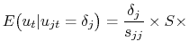
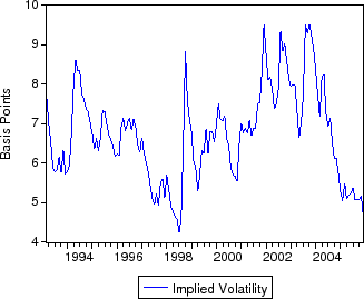
We use both primary and secondary market mortgage rates to compute our measures of mortgage rate spreads. The primary market mortgage rate is the monthly average interest rate on new 30-year fixed-rate mortgages, from Freddie Mac's Primary Mortgage Market Survey. The secondary market mortgage rate is the monthly average current-coupon yield on Fannie Mae and Freddie Mac 30-year MBS, from Bloomberg. Mortgage rate spreads are taken with respect to a duration-matched Treasury rate.¹²

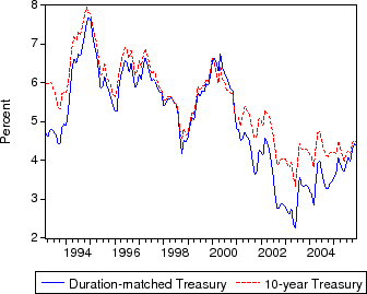
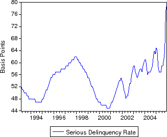
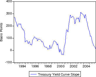
The primary risks priced into mortgage rates (but not risk-free rates) are credit risk (the risk of default) and prepayment risk (the risk of early termination). As a proxy for credit risk, we use the realized serious delinquency rate on conforming mortgages owned by Fannie Mae.¹³ We proxy prepayment risk with a measure of forward-looking interest rates and implied volatilities. In particular, we use the slope of the Treasury yield curve (1 to 10 year) and the 10-year Treasury rate. We further augment the model by including implied volatility on 10-year Treasuries as an endogenous component in the VAR. The implied volatility is calculated from the options on 10-year Treasury futures contracts.

In relating mortgage rate spreads to GSE secondary market activity data, several complications arise. First, relative to our mortgage rate spread data, MBS issuance data can be lagged. That is, some time passes between when a new homeowner locks into and closes on a mortgage, and more time passes between when the mortgage closes and when it is securitized and sold in MBS. Second, there can be lags between when a GSE commits to a mortgage purchase and when the purchase is brought onto the GSEs' books. Because the GSEs do not release enough data publicly to adjust for these lags, we control for these two issues by (1) including lagged terms in our VAR and (2) using Fannie Mae commitments as an alternative to portfolio purchases in our robustness checks.¹⁴ The lags in the VAR will then manifest the timing differences as delayed responses in our impulse response function analysis.

The expected extra return to holding mortgages once these risks have been priced is known as the option-adjusted spread (OAS). If the option-adjusted spread (OAS) on mortgages is mean-reverting, buying mortgages while the OAS is unusually high could be a profitable strategy. Rather than include an estimate of the OAS directly in our primary specification, we simply include some of the components of an OAS model. This strategy avoids any problems with including an estimated variable on the right-hand side of a regression.¹⁵

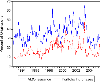
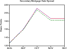
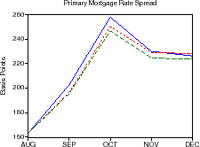
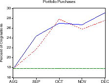
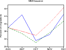
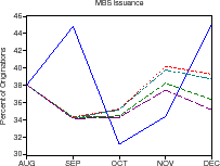
Descriptive statistics for the data are provided in table 1. Figures 1-3 plot the time series of Treasury yields and implied volatilities on 10-year Treasuries, primary and secondary mortgage rate spreads, GSE portfolio purchases and MBS issuance (relative to total originations), and the mortgage delinquency rate and the slope of the Treasury yield curve. Note that the debt crisis of late 1998 was associated with a sharp widening of spreads and volatility and increased portfolio purchases; in just two months, primary mortgage rate spreads rose about 95 basis points and portfolio purchases (relative to originations) increased about 10 percent.

4 Estimation Results

In this section we discuss our estimated generalized impulse response functions under our baseline specification. We find that unanticipated portfolio purchases have essentially no effect on mortgage rate spreads. We also show that GSE activities during the debt crisis of late 1998 were not extraordinary; further, had the GSEs not reacted to the spread widening during this period, primary and secondary mortgage rate spreads would have evolved in about the same way.

4.1 Baseline Specification

Our baseline specification is a stationary vector autoregression in which the five endogenous variables are: (1) secondary market mortgage rate spreads, (2) primary market mortgage rate spreads, (3) interest rate volatility, (4) GSE MBS issuance, and (5) GSE portfolio purchases. Our three exogenous variables are the ten-year Treasury rate, the slope of the Treasury yield curve, and the serious delinquency rate on mortgages reported by Fannie Mae. The Akaike Information Criterion (AIC) suggests that the optimal specification features two lags for the endogenous variables and one lag for the exogenous variables.¹⁶ Variable definitions and sources are explained in section 3.

We included Treasury market volatility as an endogenous variable because Perli-Sack (2003) provide evidence that mortgage hedging can amplify movements in Treasury rates. Thus the volatility of risk-free rates might itself be endogenous to secondary market prices and GSE actions. Note that volatility, taken together with the slope and level of the yield curve, contains significant information about the value of the prepayment option embedded in mortgages.

Gross MBS issuance, which is included as an endogenous variable, is not completely under the GSEs' control, especially from month to month. While it might not be a policy tool in the same way that portfolio purchases are, MBS issuance does convey information about the size of the conforming mortgage market. Also, by including it, we can more closely address the conclusions of Naranjo and Toevs.

As with many financial series, the raw endogenous variables of interest may not be stationary. Gross MBS issuance and portfolio purchases contain obvious trends; we use a natural scaling factor (total mortgage originations) to convert them into stationary variables. Our scaled variables can be interpreted as the percent of originated mortgages securitized by the GSEs and purchased by the GSEs for their own portfolios. As we discussed in section 3, the timing of our data on originations may not match the timing of our data on GSE actions; we consider this issue in our robustness testing below.

Mortgage rate spreads, the yield curve, and delinquency rates might, as shown in table 2, have unit roots in their levels. However, economic theory suggests otherwise. A unit root in spreads would suggest that any unexpected shock to spreads would be permanent, but, a priori, we expect spreads to be mean reverting. However, such spreads may revert to their long-run means only slowly, rendering unit root tests less powerful. We follow economic theory rather than strict statistical results in our baseline specification; however, we also consider a nonstationary model in our robustness tests.

As we discussed in section 2, standard identification schemes require assuming a particular shock ordering. However, assumptions about shock ordering are more likely to affect the estimated impulse response functions when the variables are strongly correlated within periods. Table 3 shows the contemporaneous correlation between estimated residuals from the reduced-form VAR. This matrix is nearly block-diagonal among mortgage rate spreads and GSE activities, which shows that the variables of interest are only weakly correlated within periods. Thus, we would expect (as we find) that choosing a particular order for the shocks does not significantly affect our results. That is, our results are robust to the choice of shock ordering because there is not much contemporaneous correlation between GSE activities and mortgage rate spreads. There is simply not very much causality to assign within a given month.

Moreover, in our baseline specification, we do not use the triangular decomposition that requires an a priori assumption about shock order. Instead, as discussed in section 2.4, we use the generalized impulse response functions (Pesarin and Shin (1998)). These impulse response functions are invariant to the ordering of variables in the VAR, and use the historical correlations among the reduced-form residuals to formulate the residual variance-covariance matrix, allowing for contemporaneous cross-correlations among the endogenous variables.

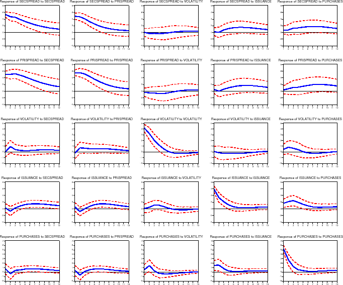
4.2 Impulse Response Functions

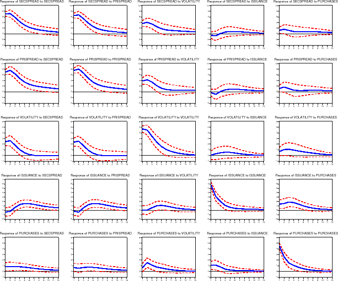
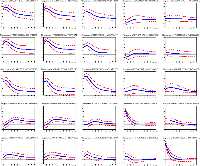
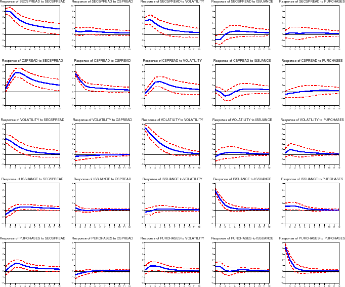
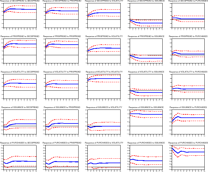
Figure 4 shows the estimated generalized impulse response functions under our baseline specification. For each variable (shown in the rows), we computed the effect of a one-standard deviation shock to each of the five equations (shown in the columns). We summarize the effect of each shock (reading down each column) in turn. The primary results of interest are shown in the top right graphs: the response of mortgage rate spreads to GSE portfolio purchases.

Effect of a Shock to the Secondary Mortgage Rate Spread.

The first column of figure 4 gives the reaction of the five endogenous variables (secondary mortgage rate spread, primary mortgage rate spread, implied volatility, gross MBS issuance, and portfolio purchases) to a one standard deviation shock to the secondary mortgage rate spread (7.0 basis points). As shown in the top row, a shock to secondary mortgage rate spread tends to be fairly persistent, with a half life of around 3 to 4 months. The second graph shows how the primary mortgage rate spread reacts to the same secondary mortgage rate spread shock; as one would expect, the primary market spread reacts strongly, increasing 7.0 basis points, and is highly correlated with the secondary mortgage rate spread. The third row shows the reaction of implied volatility on ten-year Treasuries to the shock to the secondary market spread. Volatility increases about 1/4 basis points, with a half life of about 3 months.

The bottom two graphs show the responses of GSE activities to the secondary mortgage rate shock. In effect, they show how GSE business decisions react to an unexpected widening of mortgage spreads. As shown in the fourth row, MBS issuance (measured as a share of originations) is at first essentially unchanged, but builds up to an increased 1.6 percent by the fourth month following the shock, and then slowly trails off. As shown in the bottom row, a shock to the secondary market mortgage rate spread increases the GSE portfolio purchase share of originations by 0.9 percent almost immediately, with a half life of about 6 months.

Effect of a Shock to the Primary Mortgage Rate Spread.

The second column of the figure gives the reaction of the endogenous variables to a one standard deviation shock to the primary mortgage market spread (7.6 basis points). The general patterns closely mirror the reactions to a shock to the secondary mortgage rate spread. MBS issuance (fourth row) increases by 1.6 percent of originations by 4 months after the shock, with a half life about 5 months after this (9 months after the initial shock to the primary mortgage rate spread). The initial impact of this shock is to increase the GSE portfolio purchase share of originations by 0.7 percent (fifth row), with a half life of about 8 months.

Effect of a Shock to Volatility.

The third column of the figure gives the reaction to a one standard deviation shock to implied volatility (0.5 basis points). Primary and secondary mortgage rate spreads (the top two rows) both increase following increases in volatility. Shocks to volatility itself (third row) are not very persistent, with a half life of 3 months. MBS issuance (fourth row) reacts slowly, increasing by 1.1 percent of originations by the fourth month after the shock (and a half life 3 months after this). Portfolio purchases (bottom row) increase in the months following a shock to volatility, with purchases increasing by 1.6 percent of originations one month after the initial shock (with a half life of 1 or 2 months).

Effect of a Shock to MBS Issuance.

The fourth column of the figure gives the reaction to a one standard deviation shock to gross MBS issuance (5.8 percent of originations). Primary and secondary mortgage rate spreads (the top two graphs) do not move more than a basis point away from zero; further, these movements are statistically insignificant. MBS issuance also has virtually no effect on volatility. MBS issuance itself (the fourth graph) shows little persistence, with a half life of only 1 or 2 months. As shown in the bottom graph, portfolio purchases increase by about 1.1 percent of originations with a half life of 2 or 3 months.

4.2.0.5 Effect of a Shock to Portfolio Purchases.

The final column of the figure gives the reactions to a one standard deviation shock to portfolio purchases (4.5 percent of originations). Both secondary and primary market spreads (the top two graphs) increase between 1 and 2 basis points following an unexpected increase in portfolio purchases, although these increases are not statistically different from zero, and quickly trail off (half lives are about 2 months). The middle graph shows that volatility increases by about 0.1 basis points due to the purchase shock. Interestingly, shocks to portfolio purchases push gross MBS issuance up (1.9 percent of originations) for several months (fourth graph). Portfolio purchases themselves show little persistence, with a half life of 1 or 2 months.

Effect of GSE Activities on Mortgage Rates

Based on our impulse response analysis, we estimate that if the GSEs unexpectedly increase their portfolio purchases by $10 billion (about 3.7 percent of average monthly originations during 2004), the primary and secondary mortgage rate spreads would increase 1.4 and 1.3 basis points after one month, respectively. But if the GSEs instead unexpectedly increased their securitization activity (that is, their gross issuance of MBS) by $10 billion, we estimate that primary and secondary mortgage rate spreads would decline 0.6 and 0.5 basis points, respectively. Note that none of these effects is statistically different from zero. These results suggest that GSE portfolio purchases, in particular, have economically and statistically negligible effects on mortgage rate spreads.

4.3 Counterfactual: GSEs During Financial Crisis

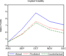
As we demonstrated, mortgage rate spreads do not react to an unexpected shock to portfolio purchases. However, we can also use our estimates to simulate how mortgage spreads would have evolved had the GSEs not followed their expected plans. These results are especially interesting during financial crises, when mortgage spreads widen abruptly. In addition, we can test how well our model predicts actual GSE behavior during financial crises; if the GSEs act to dampen crises by buying more mortgages than usual, our models should significantly underpredict the volume of mortgage purchases based on wider spreads alone. If our models predict GSE behavior fairly well during the crisis period we know that the GSEs were not (in this episode at least) "leaning against the wind" to stabilize markets in a way that our statistical work wouldn't capture because of its rarity.

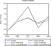
We focus on the August-October 1998 Russian debt default/LTCM crisis. In figure 5, we plot our model's predicted path for portfolio purchases and MBS issuance through this period as well as actual purchases and issuance. We also plot the results of counterfactual simulations. In these simulations, we use our estimated coefficients to predict how mortgage spreads would have evolved had portfolio purchases remained flat through the crisis.

We find that our model predicts actual portfolio purchases and MBS issuance fairly well, supporting the view that the GSEs' behavior through this financial crisis was not out of the ordinary. Further, our counterfactual simulations suggest that had the GSEs kept their portfolio purchases flat, the path of mortgage interest rates through the crisis would have followed essentially the same paths as when portfolio purchases did react to wider secondary market spreads.

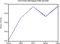
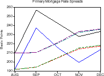
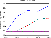
In the two months from the end of August 1998 to October 1998, secondary mortgage rate spreads widened about 85 basis points and primary mortgage rate spreads widened nearly 95 basis points. MBS issuance declined about 7 percent of originations and portfolio purchases increased by over 9 percent of originations.

During this period spreads and purchases moved much more than during normal periods. As shown in the upper-left panel of figure 5, secondary mortgage rate spreads increased about 33 basis points in September, another 52 basis points in October, before decreasing about 25 basis points in November, and remaining essentially unchanged in December.

We used our model estimates to conduct two related studies of this episode. First, we compared the actual trajectories of the endogenous variables to the predicted trajectories when we force secondary market spreads to follow their actual path over the episode, but allow all other endogenous variables to evolve as specified by the estimated model. These trajectories are given by the curves labeled "predicted" in the figure.

As shown in the upper-right panel, the model does a nice job in explaining the evolution of the primary mortgage rate spread given the shocks to the secondary mortgage rate spread, though the actual primary market spread was a little wider than our model predicted. The middle-left panel shows that GSE portfolio purchases during this period can be explained almost completely by their historical pattern of buying mortgages when mortgage rate spreads are wide, while the middle-right panel shows that the GSE MBS issuance was also fairly ordinary. The lower panel shows that implied volatility was a bit higher than predicted by the model. In all, there was nothing particularly special about the GSE actions during this period of financial market stress.

Our second experiment estimates the evolution of the endogenous variables, especially mortgage spreads, had GSE portfolio purchases been held constant. We set all variables to their August values, force portfolio purchases to be constant at their August levels, and take into account the series of shocks to secondary market spreads (from their August 1998 level). Otherwise, the endogenous variables evolve based on the estimated coefficients. These results are summarized by the curves labeled "counterfactual" in figure 5.

In the counterfactual experiment, MBS issuance is somewhat below actual (middle-right), but primary and secondary mortgage rate spreads and implied volatility are essentially the same (and perhaps slightly lower) as the model originally predicted (upper two and lower panels). The difference between our counterfactual experiment and our model's prediction is our estimate of the effect of GSE portfolio purchases on mortgage rate spreads during this period of crisis. As shown, GSE portfolio purchases appear to have had little effect on either primary or secondary mortgage rate spreads or on implied volatility.

5 Robustness Tests

Figure 4 gave the estimated impulse response functions under our baseline specification. We now estimate and report a complete set of impulse response functions under a variety of alternative specifications, data periods, and variable definitions. In particular: (1) we replace our duration-matched Treasury yields with constant-maturity yields; (2) we replace Treasury rates with swap rates; (3) we restrict the sample to 1993-1999; (4) we restrict the sample to 1993-2002; (5) we replace the Freddie Mac primary mortgage rate with the rate on jumbo mortgages taken from MIRS; (6) we replace the Freddie Mac primary mortgage rate with the rate on conforming mortgages taken from MIRS; (7) we repeat our earlier counterfactual experiment using jumbo and conforming mortgage rate spreads; (8) we dispense with our scaling factor for GSE activities and use first differences to force stationarity; (9) we take differences of our normalized measures of GSE activities; (10) we use option-adjusted spreads; (11) we use Fannie Mae commitments instead of actual purchases; and (12) we use corporate bond spreads as a proxy for credit risk. In all, our main result--that GSE portfolio purchases do not lower mortgage rate spreads--remains unchanged.

In addition to the alternative specifications reported here, we also estimated nonstationary specifications. We report results from those specifications alongside our attempts to reproduce the results of Gonzaler-Riviera (2001) Naranjo and Toevs (2002). (See section A.)

5.1 Alternative Identifying Assumptions

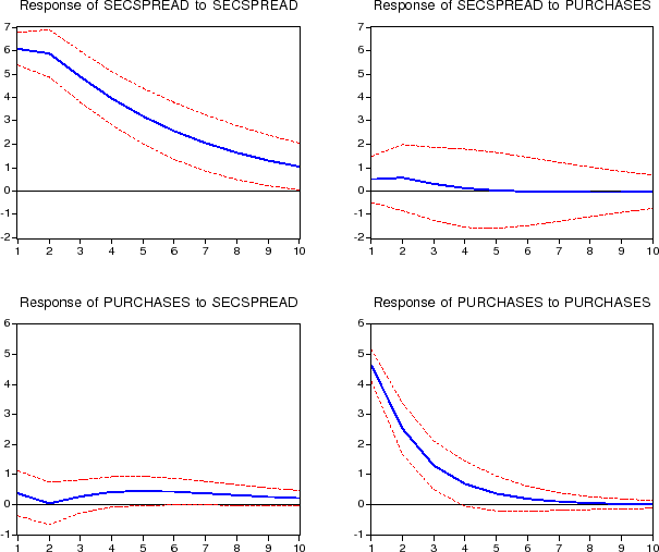
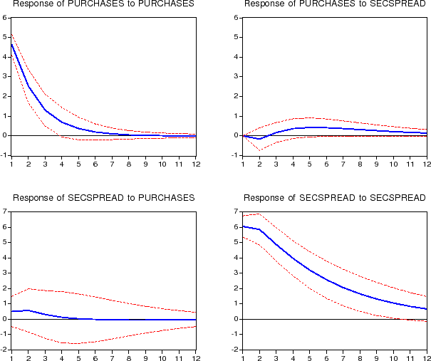
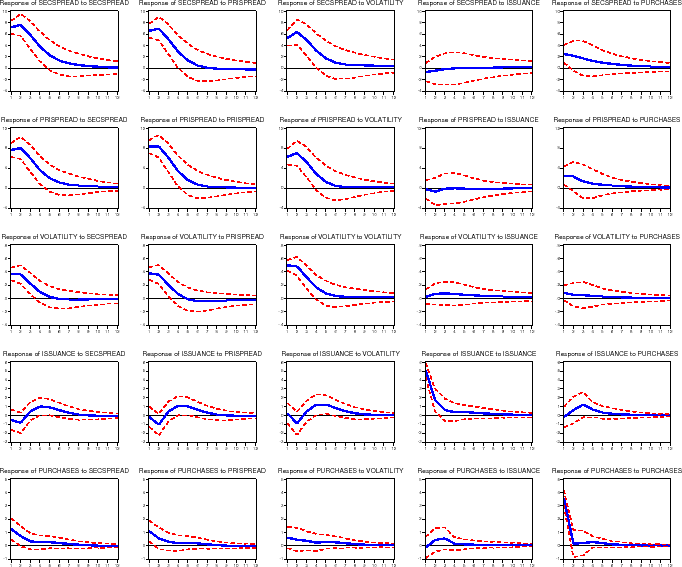
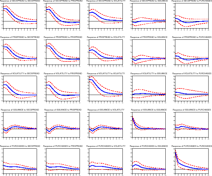
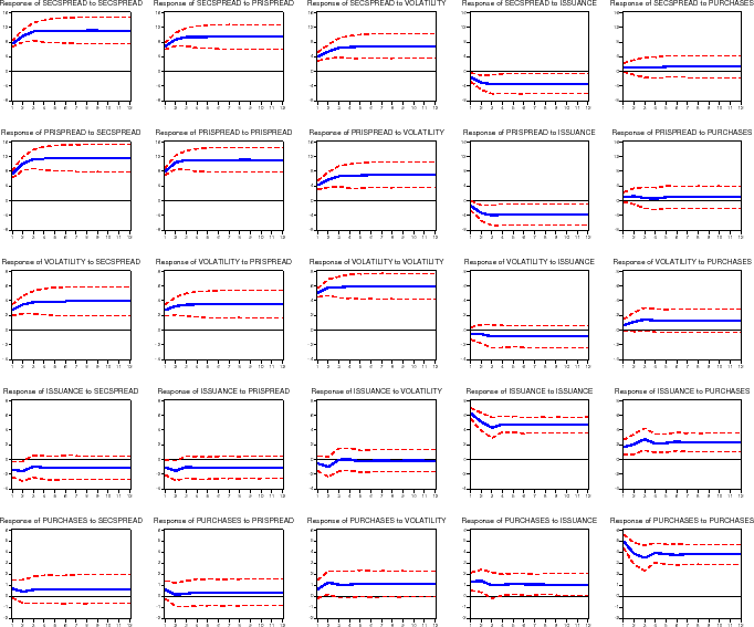
Our first robustness test is to use a triangular or Cholesky-style identification scheme in place of the Pesaran-Shin IRFs we used in our baseline specification. Triangular decompositions remain quite popular in the VAR literature, and have an obvious structural interpretation. However, with five endogenous variables there are simply too many potential triangular shock orderings to be conveniently summarized. In this section we report results after stripping our system to two endogenous variables: portfolio purchases and secondary market spreads.¹⁷

In the small system there are only two triangular decompositions: either purchases cannot react to spreads within a month, or spreads cannot react to purchases within a month. Neither of these alternatives is completely satisfying, which is why we prefer the Pesaran-Shin identification scheme. For comparison, figure 6 shows the estimated Pesaran-Shin IRFs. Figure 7 shows the estimated IRFs under the assumption that spreads cannot react to purchases within a month; figure 8 shows the estimated IRFs under the alternative assumption that purchases cannot react to spreads within a month.

Our results are broadly unchanged: purchases do not affect spreads, while spreads lead to increased purchases, perhaps with a lag of several months.

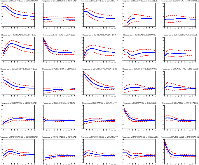
5.2 Duration-Matched versus 10-Year Treasuries

In our baseline specification we compute spreads between mortgage rates and Treasuries of the same estimated duration. Figure 9 shows the impulse-response functions for a specification in which the primary and secondary mortgage rate spreads are taken with respect to the constant-maturity 10-year Treasury rate, rather than a duration-matched Treasury rate. As shown, MBS issuance increases by 1.7 percent (of originations) by 4 months after a 7.0 basis point shock to secondary market spreads, while portfolio purchases increase by 1.4 percent (of originations) by 2 months after the shock. Mortgage rate spreads, however, show statistically negligible effects due to shocks to GSE secondary market activities.

5.3 Treasuries versus Swaps

As another alternative benchmark risk-free rate we compute spreads between mortgage rates and duration-matched swaps, rather than duration-matched Treasuries. Treasury rates are influenced by flights to quality and other factors that might not affect mortgage rates. Figure 10 shows the impulse-response functions for this specification. As shown, MBS issuance increases by 1.5 percent (of originations) by 5 or 6 months after a 5.4 basis point shock to secondary market spreads, while portfolio purchases increase by about 0.7 percent (of originations) by 5 or 6 months after the shock. Mortgage rate spreads again show little effect due to shocks to GSE secondary market activities.

5.4 1993-1999 Sample Period

Our baseline specification uses data from March 1993 to December 2005. If GSE actions were notably more effective in the earlier period, using the full sample might mask this result. Figure 11 shows the impulse-response functions estimated over 1993 to 1999. As shown, MBS issuance increases by 1.0 percent (of originations) by 3 months after a 7.2 basis point shock to secondary market spreads, while portfolio purchases increase by 1.3 percent (of originations) immediately. Mortgage rate spreads, however, show little effect due to shocks to GSE secondary market activities.

5.5 1993-2002 Sample Period

Some commentators believe that GSE actions were restrained following revelations about accounting irregularities in 2003. If financial markets reacted differently during this period of restraint, the estimated IRFs using the full sample might be artificially dampened. Figure 12 shows the impulse-response functions for a specification estimated over 1993 to 2002. As shown, MBS issuance increases by 1.1 percent (of originations) by 3 months after a 7.2 basis point shock to secondary market spreads, while portfolio purchases increase by about 1.0 percent of (originations) immediately. Mortgage rate spreads again show little effect due to shocks to GSE secondary market activities.

5.6 Jumbo Market Spread

In the next specification, we examine the effect of GSE secondary market activities on the jumbo market spread, measured as the spread between the average monthly MIRS jumbo rate and the average 10-year Treasury rate over the last five business days of the month, rather than the primary market spread.¹⁸Figure 13 shows the impulse-response functions for this specification. As shown, MBS issuance increases by 1.2 percent (of originations) by 5 months after a 8.1 basis point shock to secondary market spreads (measured as the average over the last five business days of the month), while portfolio purchases increase by 1.4 percent (of originations) by 2 months after the shock. Little effect is apparent from a (8.8 basis point) shock to the jumbo market spread. Secondary market and jumbo market spreads show little effect due to shocks to GSE portfolio purchases, but the secondary market spread exhibits a statistically significant 1.8 basis point decline due to a (5.9 percent of originations) shock to MBS issuance (this effect does not seem to flow through to new mortgage borrowers).

5.7 Conforming Market Spread

In the next specification, we examine the effect of GSE secondary market activities on the conforming market spread, rather than the jumbo market spread, measured as the spread between the average monthly MIRS conforming rate and the average 10-year Treasury rate over the last five business days of the month. Figure 14 shows the impulse-response functions for this specification. As shown, MBS issuance increases by 1.0 percent (of originations) by 4 months after a 8.1 basis point shock to secondary market spreads, while portfolio purchases increase by 1.4 percent (of originations) by 2 months after the shock. Little effect is apparent from a (5.5 basis point) shock to the conforming market spread. Secondary market and jumbo market spreads show little effect due to shocks to GSE portfolio purchases, but the secondary market spread exhibits a statistically significant 1.7 basis point decline due to a (5.8 percent of originations) shock to MBS issuance (again, this effect does not seem to flow through to new mortgage borrowers).

5.8 Jumbo and Conforming Market Spreads During Late 1998

An obvious generalization of our counterfactual experiment from section 4.3 is to replace the single primary market interest rate from Freddie Mac with the separate jumbo and conforming mortgage rates from MIRS. As shown in figure 15, our estimated models predict secondary market spreads well, but tend to underpredict both jumbo and conforming market spreads. Also, GSE secondary market activities are underestimated. When we hold GSE portfolio purchases constant over the crisis period, MBS issuance is somewhat smaller (middle-right), but primary and secondary mortgage rate spreads and volatility are essentially the same as the model originally predicted (upper two and lower panels). Once again, the difference between our counterfactual experiment and our model's prediction is our estimate of the effect of GSE portfolio purchases on mortgage rate spreads during the crisis period. As shown, GSE portfolio purchases appear to have had little effect on either primary or secondary mortgage rate spreads (or volatility).

5.9 First Differences: Unnormalized GSE Activities

Next, we consider a difference-stationary specification to address potential problems stemming from unit roots in interest rate spreads. GSE secondary market activities are measured in logs and are not normalized by HMDA originations. Figure 16 shows the cumulative impulse-response functions for this first-differences specification. As shown, MBS issuance eventually increases by 2.8 percent following a 7.4 basis point shock to secondary market spreads, while portfolio purchases increase by 8.3 percent. Mortgage rate spreads show little effect due to a 28 percent shock to GSE portfolio purchases, but show a statistically significant 3.2 to 3.4 basis point decline due to a 15 percent shock to MBS issuance.

5.10 First Differences: Normalized GSE Activities

We next consider the same difference-stationary specification, but instead of measuring GSE secondary market activities in unnormalized logs, we normalize by HMDA originations (as in our primary specification). Figure 17 shows the cumulative impulse-response functions for this first-differences specification. As shown, MBS issuance eventually decreases by 1.1 percent (of originations) following a 7.5 basis point shock to secondary market spreads, while portfolio purchases increase by only 0.6 percent (of originations). Mortgage rate spreads show little effect due to a 5 percent (of originations) shock to GSE portfolio purchases, but show a statistically significant 3.4 to 3.8 basis point decline due to a 6 percent (of originations) shock to MBS issuance.

5.11 Option-Adjusted Spreads

Next, we examine the effects of option-adjusted spreads on our results. Option-adjusted spreads obviously require an estimate of the value of the prepayment option on a mortgage. Not only are these estimates model-dependent, in practice, market participants price different mortgages using different models. Thus, although they might carry the same coupon rates, the estimated OAS on a pool of high-balance unseasoned loans will differ from the estimated OAS on a pool of low-balance seasoned loans. We used Bloomberg's estimate of the value of the prepayment option on newly issued par GSE MBS as representing the value of the prepayment option to the average borrower. We obtained data for 1997-2005 from Bloomberg and subtracted the value of the embedded option to prepay a mortgage from the unadjusted primary and secondary market spreads. Figure 18 shows the impulse-response functions for this specification. As shown, MBS issuance increases by 2.3 percent (of originations) by 3 or 4 months after a 10.4 basis point shock to the option-adjusted secondary market spread, while portfolio purchases increase by 2.2 percent (of originations) by 1 month after the shock. Option-adjusted spreads, however, show little effect due to shocks to GSE secondary market activities.

5.12 Fannie Mae Commitments

Mortgage rates might respond to news about future portfolio purchases rather than to the purchases themselves. We used Fannie Mae's commitments to purchase mortgages as proxy for news about future portfolio movements. Figure 19 shows the impulse-response functions for a specification in which Fannie Mae commitments are used in place of GSE portfolio purchases. As shown, MBS issuance increases by 1.3 percent (of originations) by 4 or 5 months after a 7.1 basis point shock to the secondary market spread, while portfolio purchases increase by 0.9 percent (of originations) immediately. Mortgage rate spreads, however, show little effect due to shocks to GSE secondary market activities.

5.13 Corporate Bond Spreads as a Proxy for Credit Risk

The credit risk measure we include in our baseline model is backward-looking. As an alternative, we used corporate bond spreads as a more forward-looking proxy for credit risk. Figure 20 shows the impulse-response functions for a specification in which the spread between Moody's BAA- and AAA-rated industrial bond yields is used instead of Fannie Mae's reported serious delinquency rate. As shown, MBS issuance increases by 1.0 percent (of originations) by 4 or 5 months after a 7.2 basis point shock to the secondary market spread, while portfolio purchases increase by 0.8 percent (of originations) almost immediately. Mortgage rate spreads, however, show little effect due to shocks to GSE secondary market activities.

6 Conclusion

We examined the empirical connection between mortgage interest rates and GSE secondary market activities, especially GSE purchases of mortgages for their own portfolios. If GSE portfolio purchases affected mortgage rates, they could stabilize mortgage markets. This benefit would flow to all mortgage market participants, not just GSE shareholders.

Earlier studies have conflicted with each other: Naranjo and Toevs (2002) conclude that GSE activities significantly affect mortgage spreads, while Gonzales-Riviera (2001) concludes that mortgage spreads drive portfolio purchases. Our findings are consistent with Gonzalez-Rivera's study, and we were unable to reproduce Naranjo and Toevs' findings.

We found that portfolio purchases have economically and statistically negligible effects on both primary and secondary mortgage rate spreads. Our results are robust to alternative identifying assumptions and to alternative model and variable specifications.

We examined the debt crisis of late 1998 and found that GSE activities generally followed the predictions of our model. Further, had the GSEs not reacted to mortgage rate spread widening through these episodes, we estimate that mortgage spreads paid by new mortgage borrowers would have evolved in about the same way.

Bibliography

Ambrose, B., M. LaCour-Little, and A. Sanders (2004).

The effect of conforming loan status on mortgage yield spreads: A loan level analysis.
Real Estate Economics 32, 541-69.

Brunnermeier, M. K. and L. H. Pedersen (2005).

Predatory trading.
The Journal of Finance 60(4), 1825-64.

Cotterman, R. F. and J. E. Pearce (1996).

The effects of the Federal National Mortgage Association and the Federal Home Loan Mortgage Corporation on conventional fixed-rate mortgage yields.
In Studies on Privatizing Fannie Mae and Freddie Mac, pp. 97-168. Washington, DC: U.S. Department of Housing and Urban Development, Office of Policy Development and Research.

Gonzalez-Rivera, G. (2001).

Linkages between secondary and primary markets for mortgages.
Journal of Fixed Income 11, 29-36.

Greenspan, A. (2005a, May 19).

Remarks by Alan Greenspan, Chairman of the Board of Governors of the Federal Reserve System, via Satellite at the Conference on Housing, Mortgage Finance, and the Macroeconomy at the Federal Reserve Bank of Atlanta.

Greenspan, A. (2005b, April 6).

Statement of Alan Greenspan, Chairman of the Board of Governors of the Federal Reserve System, before the Committee on Banking, Housing, and Urban Affairs of the United States Senate.

Hendershott, P. H. and J. D. Shilling (1989, June).

The impact of the agencies on conventional fixed-rate mortgage yields.
Journal of Real Estate Finance and Economics 2(2), 101-15.

Kolari, J. W., D. R. Fraser, and A. Anari (1998, Winter).

The effects of securitization on mortgage market yields: A cointegration analysis.
Real Estate Economics 26(4), 677-93.

Koop, G., M. H. Pesaran, and S. M. Potter (1996).

Impulse response analysis in nonlinear multivariate models.
Journal of Econometrics 74(1), 199-147.

Lucas, D. and R. McDonald (2005).

An options-based approach to evaluating the risk of Fannie Mae and Freddie Mac.
Manuscript, Department of Finance, Kellogg School, Northwestern University, Evanston IL.

McCullough, B. D., K. A. McGeary, and T. D. Harrison (2006).

Lessons from the JMCB archive.
Journal of Money, Credit, and Banking 38(4), 1093-1107.

McKenzie, J. (2002).

A reconsideration of the jumbo/non-jumbo mortgage rate differential.
Journal of Real Estate Finance and Economics 25, 197-214.

Naranjo, A. and A. Toevs (2002).

The effects of purchases of mortgages and securitization by government sponsored enterprises on mortgage yield spreads and volatility.
Journal of Real Estate Finance and Economics 25, 173-96.

Office of Management and Budget (2004).

Analytical Perspectives, Budget of the United States Government, Fiscal Year 2005.
Washington: Government Printing Office.

Office of Management and Budget (2006).

Analytical Perspectives, Budget of the United States Government, Fiscal Year 2007.
Washington: Government Printing Office.

Passmore, W., S. M. Sherlund, and G. Burgess (2005).

The effect of housing government-sponsored enterprises on mortgage rates.
Real Estate Economics 33(3), 427-463.

Perli, R. and B. Sack (2003).

Does mortgage hedging amplify movements in long-term interest rates?
Journal of Fixed Income 13(3), 7-17.

Pesaran, H. and Y. Shin (1998).

Generalized impulse response analysis in linear multivariate models.
Economics Letters 58(1), 17-29.

Roll, R. (2003).

Benefits to homeowners from mortgage portfolios retained by Fannie Mae and Freddie Mac.
Journal of Financial Services Research 23(1), 29-42.

Rothberg, J. P., F. E. Nothaft, and S. A. Gabriel (1989).

On the determinants of yield spreads between mortgage pass-through and Treasury securities.
Journal of Real Estate Finance and Economics 2(4), 301-15.

Sarno, L. and D. L. Thornton (2004).

The efficient market hypothesis and identification in structural VARs.
Federal Reserve Bank of St. Louis Review 86(1), 49-60.

**Table 1:** Descriptive Statistics
Variable	Mean	Median	Std. Dev.	Min	Max
GSE Activities (percent of originations) - MBS Issuance	36.15	34.82	9.44	19.03	65.57
GSE Activities (percent of originations) - Portfolio Purchases	18.32	17.49	7.21	7.04	47.72

Mortgage rate spreads (basis points) - Primary Market	210.12	192.91	50.55	132.58	334.30
Mortgage rate spreads (basis points) - Secondary Market	170.34	158.41	38.05	109.78	269.33

Implied volatility (basis points) - Ten-year Treasury	6.73	6.75	1.18	4.24	9.53

Explanatory variables - Yield Curve Slope¹	129.73	96.60	99.80	-38.02	313.67
Explanatory variables - Ten-year Treasury Rate²	5.49	5.60	1.05	3.33	7.95
Explanatory variables - Delinquency Rates³	54.29	55.00	5.94	45.00	79.00

NOTE. Statistics are for 154 monthly observations running from March 1993 through December 2005.

¹ Ten-year less one-year Treasury rates, expressed in basis points. Return to text

² Expressed in percent. Return to text

³ Fannie Mae "serious delinquency" rate on mortgages, expressed in basis points. Return to text

**Table 2:** Unit Root Tests
Variable	ADF Intercept	ADF Intercept+ Trend	Phillips-Perron Intercept	Phillips-Perron Intercept+ Trend
GSE Activities (percent of originations) - MBS Issuance	-4.68 $^{\star\star}$	-4.68 $^{\star\star}$	-4.56 $^{\star\star}$	-4.57 $^{\star\star}$
GSE Activities (percent of originations) - Portfolio Purchases	-4.74 $^{\star\star}$	-5.07 $^{\star\star}$	-4.61 $^{\star\star}$	-5.07 $^{\star\star}$

Mortgage Rate Spreads - Primary Market	-1.53	-1.94	-1.83	-2.38
Mortgage Rate Spreads - Secondary Market	-1.64	-1.82	-2.09	-2.37

Implied Volatility - Ten-year Treasury	-3.14 $^{\star}$	-3.10	-2.99 $^{\star}$	-2.97

Explanatory Variables - Yield Curve Slope	-1.72	-1.75	-1.71	-1.76
Explanatory Variables - Ten-year Treasury Rate	-1.69	-3.56 $^{\star}$	-1.52	-3.04
Explanatory Variables - Delinquency Rates	-0.58	-1.15	-0.16	-0.78

NOTE. Augmented Dickey-Fuller and Phillips-Perron tests of null hypotheses that indicated series have a unit root. $^{\star}$ and $^{\star\star}$ denote statistical significance at the 5- and 1-percent levels, respectively.

**Table 3:** Contemporaneous Correlation Among Reduced-Form Residuals
	Mortgage Rate Spreads Secondary Market	Mortgage Rate Spreads Primary Market	Implied Volatility	GSE Activities MBS Issuance	GSE Activities Portfolio Purchases
Secondary Mkt. Spread	1.000
Primary Mkt. Spread	0.921	1.000

Implied Volatility	0.520	0.506	1.000

MBS Issuance	-0.071	-0.035	0.010	1.000
Portfolio Purchases	0.182	0.152	0.147	0.242	1.000

NOTE. The within-period correlation between mortgage rate spreads and GSE activities (shown in the lower left portion of the matrix) are a measure of the effect of different triangular identifying assumptions on the estimated impulse response functions. Because the correlation is low, we do not expect our results to be sensitive to different identifying assumptions.

**Figure 1:** Treasury Yields and Implied Volatility
NOTE. Figure shows the time series of Treasury market data used in our analysis. The top panel gives duration-matched Treasury yields and 10-year Treasury yields; the bottom panel shows volatility on 10-year Treasuries implied by options prices.

**Figure 2:** Mortgage Rate Spreads and GSE Secondary Market Activities
NOTE. Figure shows the time series data on mortgage interest rate spreads and GSE actions used in our baseline specification. The top panel shows primary and secondary mortgage rate spreads (relative to duration-matched Treasury yields), and the bottom panel gross portfolio purchases and MBS issuance as a percentage of HMDA originations.

**Figure 3:** Mortgage Market Characteristics
NOTE. Figure gives two of the exogenous variables from our baseline specification. The top panel shows Fannie Mae's serious delinquency rate (defined as the percent of mortgages 90 days or more past due or in foreclosure). The spike at the end of our sample is related to the late-2005 hurricanes and almost completely reverses over the next six months (not in our sample). The bottom panel gives the slope of the Treasury yield curve (ten year minus one year Treasury rates).

**Figure 4:** Impulse Response Functions: Baseline Specification
NOTE. Each panel gives the effect in month for a given variable of a shock to the indicated innovation. Thus, the upper right panel shows the effect on secondary mortgage rate spreads of a one standard deviation shock to the portfolio purchase innovation.

**Figure 5:** Response During Liquidity Crisis of 1998
NOTE. Each panel gives the month-by-month effects of the liquidity shock to secondary mortgage rate spreads. Thus, the middle left graph shows that the model does well in tracing out the effects of the liquidity shock on GSE portfolio purchases. Portfolio purchases during this period had little effect on mortgage rate spreads.

**Figure 6:** Impulse Response Functions: Small System Results (Pesaran-Shin)

**Figure 7:** Impulse Response Functions: Small System Results (Cholesky/Purchases)

**Figure 8:** Impulse Response Functions: Small System Results (Cholesky/Spreads)

**Figure 9:** Impulse Response Functions: Spreads Relative to 10-Year Treasuries

**Figure 10:** Impulse Response Functions: Spreads Relative to Swaps

**Figure 11:** Impulse Response Functions: 1993-1999 Sample Period

**Figure 12:** Impulse Response Functions: 1993-2002 Sample Period

**Figure 13:** Impulse Response Functions: Jumbo Market Spread

**Figure 14:** Impulse Response Functions: Conforming Market Spread

**Figure 15:** Response During Liquidity Crisis of 1998

**Figure 16:** Cumulative Impulse Response Functions: First Differences

**Figure 17:** Cumulative Impulse Response Functions: First Differences

**Figure 18:** Impulse Response Functions: Option-Adjusted Spreads

**Figure 19:** Impulse Response Functions: Fannie Mae Commitments

**Figure 20:** Impulse Response Functions: Proxy for Credit Risk

1 Comparison with Other Studies

1a Gonzalez-Rivera (2001)

We were able to produce essentially the same results as Gonzales-Riviera (2001) when using the same methodology, specification, and data period (December 1994 to December 1999). Gonzalez-Rivera reports the cointegrating relationship ( ${}^{\star}$ denotes statistical significance at the 95 percent confidence level):

$\displaystyle \textsl{Purchases} = -51.35 + 0.554^{\star}\ \textsl{Spread}.$

Using our data over the same time period, we estimate the cointegrating relationship to be:

$\displaystyle \textsl{Purchases} = -51.47 + 0.551^{\star}\ \textsl{Spread}.$

In both cases, these estimates suggest that increases in portfolio purchases are associated with increases in mortgage market spreads. As with Gonzalez-Rivera, we also find that the error-correction term is statistically significant in the secondary market spread equation, but not statistically significant in the portfolio purchase equation. This suggests that secondary market spreads, not portfolio purchases, carry out any adjustment toward restoration of the long-run relationship. Interestingly, we cannot reject the null hypothesis of no cointegrating relationship between portfolio purchases and secondary market spreads.

Estimates of cointegrating relationships ideally require long time samples. While Gonzalez-Rivera was limited to essentially five years of data, our full sample is more than twice as long. When we include the extra six years of data in our sample (2000-2005) we estimate the long-run relationship to be:

$\displaystyle \textsl{Purchases} = 30.13 + 0.015\ \textsl{Spread}.$

Here, we find no evidence of a long-run relationship between portfolio purchases and mortgage rate spreads, as we again cannot reject the null hypothesis of no cointegrating relationship.

1b Naranjo and Toevs (2002)

In their paper, Naranjo and Toevs (2002) also posit a cointegrating relationship between mortgage market spreads and GSE activities.¹⁹ Naranjo and Toevs use mortgage rate data from the FHFB's Monthly Interest Rate Survey (MIRS) and can therefore distinguish between jumbo and conforming mortgage rates. Naranjo and Toevs use non-public data on Fannie Mae's portfolio activity going back to 1986, so we cannot exactly replicate their results. We instead attempt to reproduce their results using the same specification and comparable data. Naranjo and Toevs report the following cointegrating relationships based on their data from 1986 to 1998 ( ${}^{\star}$ denotes statistical significance at the 95 percent confidence level):

	$\displaystyle \textsl{Jumbo-Conforming Spread}$	$\displaystyle = \ensuremath{\phantom{-}}0.27^{\star}\ \textsl{Purchases}$
	$\displaystyle \textsl{Jumbo-Conforming Spread}$	$\displaystyle = \ensuremath{\phantom{-}}0.48^{\star}\ \textsl{Issuance}$
	$\displaystyle \textsl{Conforming Spread}$	$\displaystyle = - 1.74^{\star}\ \textsl{Purchases}$
	$\displaystyle \textsl{Conforming Spread}$	$\displaystyle = - 3.53^{\star}\ \textsl{Issuance}$
	$\displaystyle \textsl{Jumbo Spread}$	$\displaystyle = - 0.84^{\star}\ \textsl{Purchases}$
	$\displaystyle \textsl{Jumbo Spread}$	$\displaystyle = - 1.92^{\star}\ \textsl{Issuance}.$

These results suggest that increased purchases are associated with decreased jumbo and conforming market spreads and increased jumbo-conforming spreads. Naranjo and Toevs conclude that increased portfolio purchases decrease jumbo and conforming mortgage rate spreads, while increasing the jumbo-conforming spread.

In addition to the data we use in the main part of the paper, we also collected data on jumbo and conforming mortgage rates using the MIRS for March 1993 to December 2005. Using the data from March 1993 to December 1998--our closest match to Naranjo and Toevs' data span--we obtained the following results:

	$\displaystyle \textsl{Jumbo-Conforming Spread}$	$\displaystyle = - 0.05\ \textsl{Purchases}$
	$\displaystyle \textsl{Jumbo-Conforming Spread}$	$\displaystyle = - 1.03^{\star}\ \textsl{Issuance}$
	$\displaystyle \textsl{Conforming Spread}$	$\displaystyle = \ensuremath{\phantom{-}}0.22^{\star}\ \textsl{Purchases}$
	$\displaystyle \textsl{Conforming Spread}$	$\displaystyle = \ensuremath{\phantom{-}}0.89^{\star}\ \textsl{Issuance}$
	$\displaystyle \textsl{Jumbo Spread}$	$\displaystyle = \ensuremath{\phantom{-}}0.32\ \textsl{Purchases}$
	$\displaystyle \textsl{Jumbo Spread}$	$\displaystyle = \ensuremath{\phantom{-}}1.74^{\star}\ \textsl{Issuance}.$

We find that securitization and portfolio purchases are both positively correlated with mortgage market spreads, but negatively correlated with the jumbo-conforming spread, in the long run. Only in the fourth equation do we find evidence supporting a single cointegrating relationship.

Using our complete data set (March 1993 to December 2005), we obtained:

	$\displaystyle \textsl{Jumbo-Conforming Spread}$	$\displaystyle = - 0.01\ \textsl{Purchases}$
	$\displaystyle \textsl{Jumbo-Conforming Spread}$	$\displaystyle = \ensuremath{\phantom{-}}0.01\ \textsl{Securitization}$
	$\displaystyle \textsl{Conforming Spread}$	$\displaystyle = \ensuremath{\phantom{-}}0.43^{\star}\ \textsl{Purchases}$
	$\displaystyle \textsl{Conforming Spread}$	$\displaystyle = \ensuremath{\phantom{-}}1.62^{\star}\ \textsl{Securitization}$
	$\displaystyle \textsl{Jumbo Spread}$	$\displaystyle = \ensuremath{\phantom{-}}0.53^{\star}\ \textsl{Purchases}$
	$\displaystyle \textsl{Jumbo Spread}$	$\displaystyle = \ensuremath{\phantom{-}}1.84^{\star}\ \textsl{Securitization}.$

Again we find that securitization and portfolio purchases are both positively correlated with mortgage market spreads, but negatively correlated with the jumbo-conforming spread, in the long run. Here, we find only find evidence of a single cointegrating relationship in the fourth and sixth equations.

1c Discussion

Note that our results are perfectly consistent with the findings of Gonzales-Riviera (2001): mortgage rate spreads and GSE portfolio purchases are positively correlated. However, our results contradict those reported in Naranjo and Toevs (2002). Naranjo and Toevs find that mortgage rate spreads are negatively correlated with GSE secondary market activities, while we find a positive relationship; Naranjo and Toevs find a positive relationship between the jumbo-conforming spread and GSE secondary market activities, while we find, if anything at all, a negative relationship.

Footnotes

Revised version of FEDS 2005-7. Cathy Gessert provided excellent research assistance. We thank Ben Bernanke, Darrel Cohen, Karen Dynan, Kieran Fallon, Michael Fratantoni, Mike Gibson, Diana Hancock, Lars Peter Hansen, Paul Kupiec, Ellen Merry, Steve Oliner, Bob Pribble, Tom Tallarini, and Jonathan Wright for helpful comments and suggestions on various drafts of this paper. The opinions, analysis, and conclusions of this paper are solely those of the authors and do not necessarily reflect those of the Board of Governors of the Federal Reserve System. Return to Text

1. Source: Inside Mortgage Finance. Return to Text

2. See McKenzie, J. (2002) and Ambrose, B., M. LaCour-Little, and A. Sanders (2004). PSB2004 estimate that 7 basis points, of an estimated 16 basis point jumbo-conforming spread, are attributable to the GSE funding advantage. The other 9 basis points are attributable to different characteristics of the jumbo and conforming mortgage markets, such as compensation for differing credit and prepayment risks. Return to Text

3. The end result is mixed: some studies conclude that the GSEs decrease mortgage rate spreads--see Hendershott, P. H. and J. D. Shilling (1989, June)--while others can find no significant effects--see Rothberg, J. P., F. E. Nothaft, and S. A. Gabriel (1989). Return to Text

4. As a counterexample, inflows to mutual funds that mainly buy U.S. stocks are very highly correlated with U.S. stock price movements, even when daily data are used. In that setting, unlike ours, there is a large amount of causality to assign within a period. The estimated relationship between mutual fund flows and stock prices is strongly affected by assuming that stock prices do not react to fund flows within a given period (or vice versa). Return to Text

5. For a discussion of the difference between replication and reproduction in economics, as well as an analysis of the rates at which economic findings can be successfully replicated or reproduced, see McCullough, B. D., K. A. McGeary, and T. D. Harrison (2006). Return to Text

6. The appendix contains our efforts to reproduce the results of Naranjo and Toevs (2002) and Gonzales-Riviera (2001). Return to Text

7. In this paper, we focus only on the potential benefits brought about by GSE secondary market activities. See Lucas and McDonald (2005) for estimates of the risks to taxpayers, and Greenspan (2005a) and Office of Management and Budget (2006)2006 for assessments of the broader risks. Return to Text

8. In contrast to the accumulation of portfolio assets, the GSEs' securitization of mortgages generates few on-balance-sheet assets and results in little debt issuance. Thus, issues related to market discipline and systemic risk do not arise with respect to securitization. Return to Text

9. See Brunnermeier-Pedersen2005 for one such model. Return to Text

10. In practice, we use the Akaike Information Criterion (AIC) to determine the number of lags to include in our empirical specification--see section 4.1. Return to Text

11. See Sarno and Thornton (2004) for an example in which shock ordering affects the estimated IRFs in a standard triangular identification scheme. Return to Text

12. Durations are for Fannie Mae and Freddie Mac 30-year MBS, from Bloomberg. However, these data only go back to 1997. We therefore backcast the duration data as a function of yield curve slopes (1- to 10-year and 1- to 5-year), mortgage rates, the coupon gap, the MBA refinancing index, existing house prices, the fixed-rate adjustable-rate spread, and the adjustable-rate share of originations. Further details are available from the authors upon request. The upper panel of Figure 2 shows the duration-matched Treasury versus the 10-year Treasury yields. Return to Text

13. We realize that this is inherently a backward-looking measure. However, more forward-looking measures such as OFHEO's repeat-sales house price indexes (which would capture changes in collateral value that could be expected to translate into changes in defaults) are available only at quarterly frequencies and are also quite smooth. As an alternative, we report results using corporate bond spreads as a proxy for credit risk in the next section. Return to Text

14. We have also experimented with lagging our measure of originations in an effort to match the timing of MBS issuance and portfolio purchases, with no appreciable difference on our results. Return to Text

15. Note, however, that we report results using an OAS from 1997 through 2005 as part of our robustness checks in the appendix. These results are similar to those of our primary specification. Return to Text

16. Strict exogeneity tests suggest that our credit and prepayment risk proxies are exogenous to the system. Return to Text

17. We move implied volatility into the set of exogenous variables. Return to Text

18. We repeated the robustness tests described in this section and the next section using spreads to duration-matched Treasury rates and obtained the same results. Return to Text

19. Naranjo and Toevs do not include a constant in their long-run cointegrating relationship. Given the presence of prepayment and credit risk with mortgages, a long-run cointegrating relationship should, perhaps, include a (positive) constant. Despite this apparent omission, we continue as in Naranjo and Toevs. Return to Text

This version is optimized for use by screen readers. Descriptions for all mathematical expressions are provided in LaTex format. A printable pdf version is available. Return to Text

GSEs, Mortgage Rates, and Secondary Market Activities*