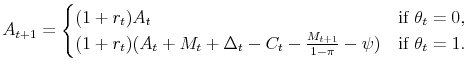
Transaction Costs and Consumption
Keywords: Transaction costs, marginal propensity to consume, consumption sensitivity
Abstract:
1 Introduction
The Rational Expectations-Permanent Income Hypothesis (RE-PIH) makes two important predictions about how consumption should respond to income changes. First, under some auxiliary assumptions, the magnitude of consumption changes in response to unanticipated and transitory income shocks should be equal to the annuity value of the shock. Second, in response to anticipated income changes, all of the adjustments in consumption should have been carried out upon the arrival of the news about anticipated future income changes, and no further adjustments are needed. Consumption should be a random walk, and its growth cannot be predicted.
Testing the validity of the RE-PIH has been an important part of economic research since the advent of the theory. After several decades of research, the literature has yielded mixed findings. Bodkin (1959) finds that the marginal propensity to consumer (MPC) out of an unanticipated transitory ("windfall") income shock can be as high as 0.9, which is well above any reasonable annuity value. In contrast, Kreinin (1961) finds that the MPC out of a windfall income shock is around 0.15, which is close to what the RE-PIH predicts. Bodkin's experiment involved small income shocks, whereas Kreinin's involved much larger ones. Taken together the findings suggest that the MPC decreases as the size of the income shock becomes larger, a relationship that cannot be explained by the RE-PIH.
Hall (1978) and Flavin (1981) challenged the random walk prediction of the RE-PIH, finding that aggregate consumption growth can be predicted by stock market returns and current income information. However, detailed household-level studies suggest that consumption responds only to small anticipated income changes; little excess sensitivity has been detected when the income shocks are large.
Various explanations have been offered for a large MPC out of windfall income and for an excess sensitivity in response to anticipated income changes. However, explanations for the different response to large and small income shocks are lacking. The present paper introduces a model predicting (1) small windfall income shocks induce a large MPC, (2) the MPC decreases as the shock becomes larger, and (3) consumption exhibits excess sensitivity in response to anticipated income changes but only when the changes are small.
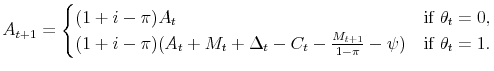
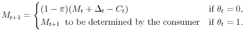
The logic of the model is as follows: In a cash-in-advance economy, a consumer can hold cash and illiquid assets (hereafter assets). The nominal interest rate is zero on cash and positive on assets. Only cash can be used to purchase consumption goods. The consumer has to pay a transaction cost to transfer wealth between cash and assets. Assume that the transaction cost is a fixed fee that does not depend on the amount of the transaction. The consumer will choose to pay the transaction cost only if income shocks have made the consumer's cash balance too low or too high relative to the individual's unconstrained optimal consumption level. A cash balance that is too low will severely constrain consumption and will cause the consumer to withdraw some money from assets to finance consumption. Likewise, a balance of (non-interest-bearing) cash that is too high will cause the consumer to transfer most of the extra cash into the asset account.
Conditional on expected future labor income and current asset holdings, there is an s-S band of cash holdings within which the consumer will choose not to transfer wealth. Optimal consumption - as a function of cash balance holdings - will not be differentiable globally. Nor is it differentiable within the no-transaction band. The consumption function is not even continuous. In particular, there are two segments of the optimal consumption function within the band. To the left of the band, the consumer has a cash holding level that is lower than the unconstrained optimal consumption level. Hence, within this region of cash holding, the MPC out of one additional dollar will be exactly equal to one. When the cash balance has increased to such a level that the consumer is no longer cash constrained, the MPC within the band is still higher than that out of the band. The reason is that if the consumer does not spend all of the cash in hand, the consumer will not receive any return on the cash saved, and may even suffer inflation loss. Therefore, by holding cash in hand, current consumption will be higher, and the profile of consumption growth will be flatter. Overall, the average MPC within the band is higher than that out of the band. As I will show later in the paper, the probability of being within the band is quite large. Only a large income shock will push the consumer out of the band. In other words, the model predicts that a small windfall income shock may be associated with a very high MPC, and that the MPC decreases as the income shocks increase.
If the consumer knows that income will be higher next period and the shock is not too large, a cash-constrained consumer will not pay the transaction cost to withdraw money from the asset account to increase current consumption. However, when the future income change is sufficiently large, it is always optimal for the consumer to pay the transaction cost and change current consumption. Therefore, an econometrician who uses cross-sectional data to test excess sensitivity will find that the Euler equation does not hold when the anticipated income changes are small, but that the Euler equation does hold when the income changes are large.
It is important to distinguish the cash constraint the consumer faces here from liquidity constraints as typically characterized in the literature. The cash constraint is endogenous in the model of this paper and the consumer optimally chooses to be constrained under some states and not under others. The liquidity constraint is exogenous, and the consumer cannot choose whether to be constrained. In my model the consumer faces a single lifetime budget constraint and is allowed to have a negative level of asset holding, whereas a negative asset balance is not permitted for a liquidity constrained consumer. Finally, being cash constrained for the current period has little predictive power for whether the consumer will be constrained next period, whereas the liquidity constraint is typically persistent.
The model is rich: It explains not only the stylized facts mentioned above but also yields some other findings that challenge the predictions of conventional models. For example, it sheds some light on the demand for liquid assets - in my model, cash. When the consumer transfers wealth between cash and illiquid assets, the consumer still wants to hold some cash into the next period even though cash does not accrue any interest. By choosing the optimum amount of cash to hold over periods, the consumer can minimize the probability of having to pay the transaction cost again in the next period. Moreover, holding some extra cash will also reduce the probability of being cash constrained when the consumer chooses not to transfer. I will call this type of demand for cash the precautionary demand for cash.
If the model is extended to allow for stochastic asset returns, the consumer will have two types of income shocks: one from labor income and the other one from the asset market. I show that this feature weakens the correlation between contemporaneous consumption growth and asset returns and thus helps explain the equity return premium puzzle; it also produces a correlation between consumption growth and lagged asset returns that is consistent with the findings by Hall (1978). Infrequent adjustment of consumption with respect to asset return shocks is also predicted by the models of Gabaix and Laibson (2001) and Reis (2006). However, the most important distinction between the model in this paper and theirs is that consumption adjustment is state dependent in the current model, whereas it is time dependent in Gabaix and Laibson (2001) and Reis (2006).
The paper will proceed as follows: Section 2 reviews the studies of the MPC out of windfall income shocks and excess sensitivities. I also discuss why the models of liquidity constraints are unable to provide complete explanations for the findings. Section 3 discusses the transaction cost in more detail and sets up the model with only labor income risk. Section 4 provides numerical solutions for the model with the benchmark parameters. In Section 5, I use the simulation results to show that the current model can replicate the stylized facts mentioned above. I also show simulation results describing the precautionary demand for cash, and I explore the sensitivity of the model by varying the parameters. Section 6 extends the model by allowing for risky asset return and discusses whether and to what extent it helps explain the equity premium puzzle. Section 7 concludes and sets up a future research agenda.
2 Evidence on the MPC and Excess Sensitivities
I will first review the evidence that (1) when the income shock is small, the MPC is much larger than what the RE-PIH predicts, and (2) the MPC tends to increase as the size of the windfall income shock decreases. Next I review the evidence of excess sensitivity in consumption in response to anticipated income changes. The literature suggests that such excess sensitivity can be detected only when the anticipated income changes are small. Finally, I briefly review the literature on liquidity constraints and argue that liquidity constraints cannot completely reconcile all of these contradictions. The literature reviewed in this section is summarized in table 1.
2.1 The MPC out of Windfall Income
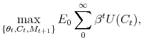
I begin with replicating the results of the baseline RE-PIH model. In this model, the representative consumer maximizes lifetime utility
 |
(1) |
subject to the intertemporal budget constraint
| (2) |
where
 . The first-order condition (FOC) can be summarized as the Euler equation,
| (3) |
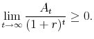
with a transversality condition,
 |
(4) |
If we further assume that the utility function is quadratic, then the solution for the consumption level under a stochastic future income process is equivalent to the solution to the above problem without uncertainty. The optimal consumption level depends only on the discounted expected income, a condition known as the certainty equivalence solution, expressed as
![\displaystyle C^{CEQ}=\frac{r}{1+r} \left[E_0 \; \sum_{t=0}^{\infty} \frac{Y_t}{(1+r)^t}+A_0\right].](img10.gif) |
(5) |
Consumption in each period is at the same level and is equal to the annuity value of the lifetime sum of human and nonhuman wealth. If ![]() unexpectedly increases by $1,
unexpectedly increases by $1, ![]() will increase by
will increase by
![]() dollar. The value is exactly the MPC out of windfall income that is predicted by the RE-PIH and is equal to the annuity value of the shock. For a reasonable level
of
dollar. The value is exactly the MPC out of windfall income that is predicted by the RE-PIH and is equal to the annuity value of the shock. For a reasonable level
of ![]() ,
,
![]() should not be greater than 10 percent.
should not be greater than 10 percent.
Bodkin (1959) examines some U.S. veterans who, in the 1950s, received unanticipated payments from the National Service Life Insurance Fund. Bodkin estimates that the MPC from these payments ranged from 0.7 to 0.9.1 This result is viewed as a challenge to the PIH as no realistic value of ![]() can generate an annuity as high as that. In
contrast, Kreinin (1961) finds that for the Israelis who received reparations payments from Germany in 1957, also an unanticipated income shock, the MPC was around 0.15; that number is easier to reconcile with the RE-PIH predictions. Finally, Hall and Mishkin (1982) estimate that the MPC out of
transitory income relative to the MPC out of lifetime income is 0.29. For a sufficiently large MPC out of lifetime income, Hall and Mishkin's estimate of the MPC out of transitory income is also very large and hard to be reconciled with the PIH predictions.
can generate an annuity as high as that. In
contrast, Kreinin (1961) finds that for the Israelis who received reparations payments from Germany in 1957, also an unanticipated income shock, the MPC was around 0.15; that number is easier to reconcile with the RE-PIH predictions. Finally, Hall and Mishkin (1982) estimate that the MPC out of
transitory income relative to the MPC out of lifetime income is 0.29. For a sufficiently large MPC out of lifetime income, Hall and Mishkin's estimate of the MPC out of transitory income is also very large and hard to be reconciled with the PIH predictions.
One of the key differences between the Bodkin and Kreinin studies is that the former involved payments that were less than 10 precent of the consumer's annual income, whereas the latter involved a much larger payment that was equal to about one year's income. Although Kreinin (1961) does not find direct evidence that the size of the shock was the reason for such a big discrepancy in estimated MPC, a later study by Landsberger (1966) lends strong support to this possibility. Landsberger divides the sample of the Israelis who received the windfall income into quintiles according to the ratio of the windfall income to their regular income. He finds that the MPC decreases consistently from the group with the lowest ratio to the group with the highest ratio. He also reports that for the group with the lowest ratio, the estimated MPC is extremely high. Bodkin (1966) did the similar estimation with the veteran dataset and cannot reject Landsberger's findings.2
2.2 Excess Sensitivities to Anticipated Income Changes
Consider the Euler equation (3). A key implication is that current consumption growth should not be correlated with any information that is available before the current period. This condition, which holds for all utility functions, is Hall's celebrated random walk hypothesis. It is also known as the orthogonality condition. In particular, consumption growth should not be correlated with expected income growth. Many authors, however, have found that it does not hold unconditionally in the data. Hall (1978) and Flavin (1981) challenge the orthogonality condition with aggregate data. Similarly, Wilcox (1989), using aggregate data, shows that the announced increases of social security benefits have significant effects on consumption at the monthly frequency because the benefits increases have been announced at least six weeks prior to payments.
As better survey data have become available, there has been an increasing volume of studies that test the orthogonality condition in natural experiments that use household-level data. Souleles (1999) showed that household consumption is excessively sensitive to tax refunds, an anticipated income shock. He found significantly higher consumption for households who received tax refund in the refund quarter, compared with the consumption of those who received their refunds in the previous quarter. Souleles (2002) studies how households' consumption responded to the second phase of the so-called "Reagan tax cuts". These tax cuts were implemented in August 1981 but were announced long before this time. Again, consumption was found to be excessively sensitive to the tax cuts at the time they went into effect. Parker (1999) shows that consumption is excessively sensitive to another source of anticipated income changes - regular changes in Social Security tax withholding. After an individual's Social Security tax withholding amount reaches a specified limit in a given calendar year, take-home pay increases. Parker finds that consumption responds to this income change significantly, even though the income change is expected.
One common characteristic of the anticipated income changes just discussed is that they are relatively small. In Souleles (1999) the sample mean of tax refund is $874 and the median is $561. In Souleles (2002), the mean change in tax withholding is about $117 per quarter, and the median is $95. In Parker (1999), the Social Security tax rate had been between 6.13 percent and 7.5 percent over various years in his sample.
The findings about excessive sensitivity are different when income changes are large. Hsieh (2003) uses the Consumer Expenditure Survey to show that the consumption of the Alaskan residents is not responsive to the receipt of oil fund royalties. These payments are anticipated and large: the average is well above $2,000 for each household. Similarly, Souleles (2000) finds that the consumption in autumn of parents who send their children to college are not affected by the tuition payments, which are also anticipated and large.
2.3 Can Liquidity Constraints Explain Everything?
One often-proposed explanation for the findings reviewed above is that not all consumers can borrow freely, that is they face liquidity constraints. If the consumer cannot borrow, or at least cannot borrow as much as she wants, the Euler equation may not hold at all times. Typically, when the consumer is liquidity constrained, consumption will be lower than the unconstrained optimal level. Therefore, windfall income will increase consumption by more than what the PIH predicts, and news about higher future income will not lead to a higher current consumption level.
Empirical tests of the liquidity constraint hypothesis have lent mixed support to the theory. Souleles (1999) finds evidence supporting the liquidity constraint model, but Souleles (2002) and Parker (1999) find no evidence that liquidity constraints can help explain the excess sensitivity. Using the Panel Study of Income Dynamics (PSID) data, Zeldes (1989a) finds that, for some criteria for identifying liquidity constraints, the Euler equation does not hold for the constrained consumers, but for other criteria, the estimates are not significant. Runkle (1990) uses the same data source and finds no evidence for liquidity constraints.
Another study that does not support the liquidity constraint model is Shapiro and Slemrod (2003). They survey households' plans to spend their 2001 tax rebate. They find that for households with income between zero and $20,000, 17.6 percent of them said that they would spend the tax rebate, whereas for households with income above $75,000, 24 percent said that they would spend the tax rebate. Higher income households' greater propensity to spend the same windfall amount that the lower-income households received is not explained by RE-PIH, nor is it explained by the liquidity constraints model.
The evidence suggests some limits to the ability of liquidity constraints in explaining such findings. First, to explain the observed excess sensitivity to predictable income changes, note that such income changes must be predictable not only by the consumers but also by the econometrician. It is then not unrealistic to assume that the creditor is also able to predict the income changes of the consumer who is applying for a loan. If, indeed, the creditor can predict that consumer's income of next period will increase, it is likely that the consumer will get the loan and not be constrained.Finally, in the case of a windfall income shock, liquidity constraints do not imply very high MPCs, unless the consumer is constrained only for the current period. Zeldes (1989a) notes that the Euler equation might still hold for the liquidity constrained consumer, as she should want to be equally distant from the optimal consumption level in all of the constrained periods and thus will still try to smooth consumption. As a result, as long as the consumer realizes that the constraint will last some sufficiently long time, the MPC out of windfall income should not be too large.
2.4 Can Behavioral Models Explain the Puzzles?
There are certainly many good behavioral models that shed light on the consumption puzzles. For instance, to produce an increase in MPC when the size of windfall income shocks decreases, the so-called mental accounting models do a good job (for example, Thaler, 1992). Costly self-control also provides a good explanation. If self-control is costly, it is worthwhile to exert self-control only when the temptation to consume (windfall income) is large (see Benhabib and Bisin 2002). However, I do not pursue these behavioral approaches in this paper.
3.1 The Environment
I assume that the consumer lives in a cash-in-advance economy. The consumer can hold either cash or assets. The nominal interest rate for cash is zero. For the time being, I assume that the asset bears a risk free real interest rate, ![]() . The nominal interest rate,
. The nominal interest rate, ![]() , is equal to
, is equal to ![]() , where
, where ![]() is the inflation rate. Interest is assumed to be accrued from the end of one period to the beginning of the next. In the Section 6, I will allow for stochastic
rates of return. All labor income comes in the form of cash. After receiving labor income, the consumer simultaneously decides whether to transfer wealth between cash and assets and how much to consume. The consumer wants to make a transfer in either of two cases. First, because the cash-in-advance
assumption requires that consumption in any period not be greater than cash holding in that period, if the desired level of consumption is greater than the cash holding, the consumer will withdraw money from the asset account. Second, if substantial cash is left in hand after paying for
consumption, the consumer will save the extra cash in asset account. The key assumption of the model is that the consumer has to pay a transaction fee for any transfer between cash and assets. When transferring wealth after receipt of labor income, the consumer also has to decide how much cash to
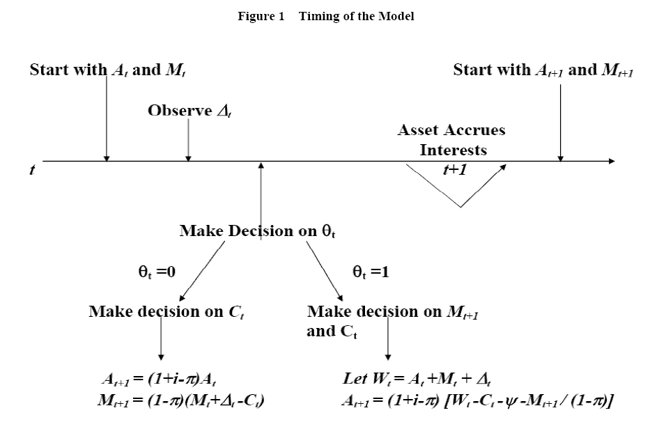
hold after the transfer.3 Figure 1 illustrates the timing of the model.
is the inflation rate. Interest is assumed to be accrued from the end of one period to the beginning of the next. In the Section 6, I will allow for stochastic
rates of return. All labor income comes in the form of cash. After receiving labor income, the consumer simultaneously decides whether to transfer wealth between cash and assets and how much to consume. The consumer wants to make a transfer in either of two cases. First, because the cash-in-advance
assumption requires that consumption in any period not be greater than cash holding in that period, if the desired level of consumption is greater than the cash holding, the consumer will withdraw money from the asset account. Second, if substantial cash is left in hand after paying for
consumption, the consumer will save the extra cash in asset account. The key assumption of the model is that the consumer has to pay a transaction fee for any transfer between cash and assets. When transferring wealth after receipt of labor income, the consumer also has to decide how much cash to
hold after the transfer.3 Figure 1 illustrates the timing of the model.
3.2 Discussion of the Transaction Cost
The categories of cash and assets broadly correspond to accounts in the real world. What I refer to as cash in my model includes cash, checking account balances, saving account balances, other account balances that can be used to purchase goods directly, and other assets that can be converted to cash with very low cost. The asset account in my model includes stocks, mutual funds, pensions, and other assets that are rather costly to convert to cash. Some of the instruments that I label as cash do bear some interest, but the rate of return is not as high as those I label as assets.
If there is no transaction cost, theory predicts that the portfolio should be adjusted continuously, and the first-best portfolio is always achieved. In real life, however, each investor trades only sporadically. Odean (1999) reports that the users of some discounted brokerage accounts trade, on average, 1.44 times per year. He also reports that this trading frequency, after taking into account of the brokerage fee the consumer has to pay for each trade, leads to suboptimal returns. Therefore, the optimal trading frequency must be even lower than 1.44 times per year. Agnew, Balduzzi and Sunden (2003) find that some 401(K) participants reshuffle their portfolio at an even lower average frequency - 0.26 times per year. Barber and Odean(2000) calculate the theoretically optimal trading frequency for reasonable levels of transaction costs, and they find that the number of trades per year should be within the range of 0.17 to 0.5 when the transaction cost varies from 0.01 percent to 0.1 percent of the portfolio value.
What are these transaction costs? The most observable and direct cost is the brokerage fee. Typically, the individual investor pays the brokerage firm $15 to $30 per transaction. The fee is by no means the only component of the transaction cost, as evidenced by people trading very infrequently in their 401(K) accounts, which charge no explicit fee. Implicit costs may include the time an investor needs to spend on market research and the effort of placing the order. The imperfect liquidity of some financial vehicles can also be associated with a transaction cost. For instance, long-term saving accounts have higher interest rates. They do, however, carry a large financial penalty for withdrawal. Another example is a house, which can be viewed as an asset with extremely high transaction costs to convert to cash.
3.3 Setup of the Model
The following notations are used in the model:
![]() is the consumption in period
is the consumption in period ![]()
![]() is a binary variable that indicates whether the consumer pays the transaction cost
is a binary variable that indicates whether the consumer pays the transaction cost
![]() if the consumer does and
if the consumer does and
![]() if the consumer does not
if the consumer does not
![]() is the real cash holding before receiving the labor income
is the real cash holding before receiving the labor income
![]() is the real balance of the asset account
is the real balance of the asset account
![]() is the real value of labor income
is the real value of labor income
![]() is the coefficient of relative risk aversion (CRRA)
is the coefficient of relative risk aversion (CRRA)
![]() is the nominal interest rate
is the nominal interest rate
![]() is the inflation rate
is the inflation rate
![]() is the real interest rate
is the real interest rate
![]() is the transaction cost
is the transaction cost
The consumer has to solve the optimization problem as follows,
 |
(6) |
subject to
 |
(7) |
 |
(8) |
| (9) |
 |
(10) |
Because the three control variables are jointly determined at time ![]() , I write the maximization problem with respect to the vector of
, I write the maximization problem with respect to the vector of
![]() . I assume a CRRA type of utility function,
. I assume a CRRA type of utility function,
 . For brevity and computational simplicity, this optimization problem is represented as the following Bellman equations,
| (11) |
where
| (12) |
and
| (13) |
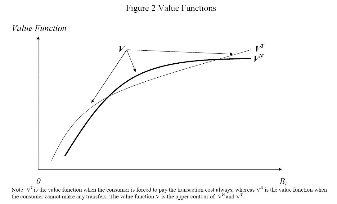
In this system, we have three value functions:
![]() , and
, and ![]() .
. ![]() is the solution to the whole optimization problem,
is the solution to the whole optimization problem, ![]() is the solution to the problem when the consumer is not allowed to transfer
wealth between cash and assets in the current period, and
is the solution to the problem when the consumer is not allowed to transfer
wealth between cash and assets in the current period, and ![]() is the solution to the problem when the consumer is forced to pay the transaction cost and make a
transfer in the current period
is the solution to the problem when the consumer is forced to pay the transaction cost and make a
transfer in the current period
![]() and
and![]() regardless of optimality.4In the regime in which the consumer is not allowed to transfer wealth, the control variable is simply
regardless of optimality.4In the regime in which the consumer is not allowed to transfer wealth, the control variable is simply ![]() , whereas in the regime of a forced transfer the consumer has to simultaneously choose
, whereas in the regime of a forced transfer the consumer has to simultaneously choose ![]() and
and ![]() . The consumption policy functions for equations (12) and (13) are denoted as
. The consumption policy functions for equations (12) and (13) are denoted as
![]() and
and
![]() , respectively. The value function,
, respectively. The value function, ![]() , is the upper
contour of
, is the upper
contour of ![]() and
and ![]() . The consumer decides
. The consumer decides ![]() as
as
 |
(14) |
which is obvious.
The motion of state variables ![]() and
and ![]() follows equations (7) and (8).
Equation (7) shows that when
follows equations (7) and (8).
Equation (7) shows that when
![]() , asset
, asset ![]() is intact in period
is intact in period ![]() , and real interest,
, and real interest, ![]() , accrues between period
, accrues between period ![]() and
and ![]() .
. ![]() is simply equal to
is simply equal to
![]() . Equation (8) shows that after making the consumption expenditure, the consumer will carry a real cash balance
. Equation (8) shows that after making the consumption expenditure, the consumer will carry a real cash balance
![]() into the period
into the period ![]() . When
. When
![]() , consumer will either withdraw cash or save cash. If the consumer chooses to consume the amount
, consumer will either withdraw cash or save cash. If the consumer chooses to consume the amount ![]() and to carry a real cash balance,
and to carry a real cash balance, ![]() , into the next period,
, into the next period,
![]() will be left in the asset account. In this case,
will be left in the asset account. In this case, ![]() becomes a control variable that has to be pinned down by the consumer. Equation (9) is the cash-in-advance constraint. If
becomes a control variable that has to be pinned down by the consumer. Equation (9) is the cash-in-advance constraint. If
![]() , consumption in period
, consumption in period ![]() will be constrained by the amount of cash the
consumer holds after receiving labor income, which is equal to
will be constrained by the amount of cash the
consumer holds after receiving labor income, which is equal to
![]() .5
.5
3.4 Characterizations of the Solution
It is well known that for the models of dynamic consumption optimization with stochastic income, the analytical solutions are not attainable except for very few situations, such as when the utility function is quadratic. Because of the nonlinearity in my model, even the assumption of quadratic utility function does not lead to a tidy closed form solution. In the next section I will solve the model using a numerical technique. In this section, I will characterize the solution.
Proof: Because ![]() , the existence of the solution is established by Theorem 9.6 in Lucas and Stokey (1989).
, the existence of the solution is established by Theorem 9.6 in Lucas and Stokey (1989).
Assume that the value functions are differentiable, so the first-order condition (FOC) for equation (12) is
![\displaystyle U'(C_t) - \beta (1-\pi) \frac{\partial}{\partial M_{t+1}} \; E_{\Delta_{t+1}} [V(A_{t+1}, \: M_{t+1}, \: \Delta_{t+1})] \geq 0.](img66.gif) |
(15) |
This FOC suggests that, if prevented from transferring wealth, the consumer should set the marginal utility from current consumption derived from cash equal to the discounted future marginal value derived from cash holdings. Without the ability to transfer wealth, the consumer might be cash constrained. In this case, the inequality holds. For equation (13), the FOC of
![\displaystyle U'(C_t) - \beta(1+i-\pi)\frac{\partial}{\partial A_{t+1}}E_{\Delta_{t+1}}[V(A_{t+1}, M_{t+1}, \Delta_{t+1}) ] = 0.](img67.gif)
And the FOC of the real cash balance at the beginning of next period, ![]() , is
, is
![\displaystyle (1+i-\pi)\frac{\partial}{\partial A_{t+1}}E_{\Delta_{t+1}}[V(A_{t+1}, M_{t+1}, \Delta_{t+1}] = (1-\pi)\frac{\partial}{\partial M_{t+1}}E_{\Delta_{t+1}}[V(A_{t+1}, M_{t+1}, \Delta_{t+1})].](img68.gif)
FOC equation (16) says that when paying a transaction cost, the consumer should, at the margin, be indifferent between consuming another dollar or saving it distributed optimally between assets,
In comparing the Euler equations (15) and (16), we find that the marginal value of saved cash in period ![]() is multiplied by
is multiplied by ![]() in the regime of no wealth transfer, whereas in the regime of a forced wealth transfer, the marginal value of saved asset is multiplied by
in the regime of no wealth transfer, whereas in the regime of a forced wealth transfer, the marginal value of saved asset is multiplied by ![]() . Therefore, the first case leads to a stronger incentive to increase current consumption and reduce future consumption growth.
. Therefore, the first case leads to a stronger incentive to increase current consumption and reduce future consumption growth.
Now I characterize the value functions. We are interested in the characteristics of both the value functions
![]() and
and
![]() . Labor income arrives in the form of cash only. After receiving that labor income, the consumer no longer has to distinguish between
. Labor income arrives in the form of cash only. After receiving that labor income, the consumer no longer has to distinguish between ![]() and
and ![]() . Therefore, we can rewrite the value functions as
. Therefore, we can rewrite the value functions as
![]() ,
,
![]() and
and
![]() , where
, where
![]() denotes cash in hand. Moreover, if paying a transaction cost, the consumer is indifferent to placing income in cash or assets, and we can define
denotes cash in hand. Moreover, if paying a transaction cost, the consumer is indifferent to placing income in cash or assets, and we can define
![]() as the wealth in hand after the transaction. We have the following proposition:
as the wealth in hand after the transaction. We have the following proposition:
We can write
![]() and
and
![]() . For the
. For the ![]() case, there still exists the saving
threshold
case, there still exists the saving
threshold
![]() , but there is no withdrawal threshold
, but there is no withdrawal threshold
![]() because the consumer has no assets left after paying the transaction cost. For such cases, the s-S rule degenerates to a single-direction rule. Also,
see the appendix for a discussion of the differentiability and concavity of the value function
because the consumer has no assets left after paying the transaction cost. For such cases, the s-S rule degenerates to a single-direction rule. Also,
see the appendix for a discussion of the differentiability and concavity of the value function ![]() .
.
Now I characterize the policy function
![]() . I focus on the property of the policy function for a given
. I focus on the property of the policy function for a given ![]() and
varying
and
varying ![]() .
.
 |
(18) |
where
Proposition 3 holds by definition and optimality. It highlights the existence of the region within which the MPC = 1.
Finally, I characterize the policy function for ![]() . Recall that with transaction costs, the consumer has to choose the optimum amount of cash to carry into the next period to minimize
the probability of having to pay the transaction cost again. Suppose that after paying for the transaction cost and the cost of consumption in period
. Recall that with transaction costs, the consumer has to choose the optimum amount of cash to carry into the next period to minimize
the probability of having to pay the transaction cost again. Suppose that after paying for the transaction cost and the cost of consumption in period ![]() , the consumer has
, the consumer has ![]() left. The consumer has to decide how much of
left. The consumer has to decide how much of ![]() to hold in assets and how much in cash.
Suppose that the consumer has a very small
to hold in assets and how much in cash.
Suppose that the consumer has a very small ![]() relative to the expected labor income of next period. Then it is very likely that the consumer has to pay the transaction cost next period no
matter how much cash is being carried from period
relative to the expected labor income of next period. Then it is very likely that the consumer has to pay the transaction cost next period no
matter how much cash is being carried from period ![]() into
into ![]() . The reason for that
is the consumer's level of savings is far below the target level of savings, which is discussed in the literature on precautionary saving (for example, Carroll, 1992 and 1997). The consumer has to save more in subsequent periods to restore the target level of savings. In such a situation the
consumer should put all of
. The reason for that
is the consumer's level of savings is far below the target level of savings, which is discussed in the literature on precautionary saving (for example, Carroll, 1992 and 1997). The consumer has to save more in subsequent periods to restore the target level of savings. In such a situation the
consumer should put all of ![]() into the asset account. Similarly,
into the asset account. Similarly, ![]() is very
large and it is higher than the target level of savings, the consumer should run down savings and increase consumption in the following period. Hence it is highly probable that consumption will exceed labor income in the next period. To avoid paying the transaction cost again next period, the
consumer has to carry an amount of cash that is close to the difference between consumption and income of next period. However, if this difference is too large, holding such amount of cash will not be optimal because the interest loss is too large (even larger than
is very
large and it is higher than the target level of savings, the consumer should run down savings and increase consumption in the following period. Hence it is highly probable that consumption will exceed labor income in the next period. To avoid paying the transaction cost again next period, the
consumer has to carry an amount of cash that is close to the difference between consumption and income of next period. However, if this difference is too large, holding such amount of cash will not be optimal because the interest loss is too large (even larger than ![]() ). In this case, the consumer should hold all of
). In this case, the consumer should hold all of ![]() in assets and make a transfer next period. Therefore,
in assets and make a transfer next period. Therefore,
![]() if
if ![]() is very small or very large. Otherwise,
is very small or very large. Otherwise, ![]() increases with
increases with ![]() .7
.7
4 Numerical Solution to the Model
Since I want to isolate the effects of the transaction cost from the effects of the liquidity constraint, in the baseline model, I assume a stochastic income process that leaves the consumer with no future income against which to borrow. I assume that the distribution of labor income,
![]() , has a positive probability of equalling to zero,
, has a positive probability of equalling to zero,
![]() . As the income in all future periods can be equal to zero (even with a very small probability), the discounted sum of minimum future income is zero. The model will be calibrated
quarterly because most micro level empirical studies use quarterly data. For simplicity, I assume that labor income is
. As the income in all future periods can be equal to zero (even with a very small probability), the discounted sum of minimum future income is zero. The model will be calibrated
quarterly because most micro level empirical studies use quarterly data. For simplicity, I assume that labor income is ![]() over time. Table 2 summarizes the baseline values of the
parameters.
over time. Table 2 summarizes the baseline values of the
parameters.
I assume that ![]() to prevent the consumer from accumulating assets without bound. This restriction is what Deaton (1992) and Carroll (1997) term the impatience condition in a
simplified environment. Setting
to prevent the consumer from accumulating assets without bound. This restriction is what Deaton (1992) and Carroll (1997) term the impatience condition in a
simplified environment. Setting ![]() at 0.015 gives us a 6 percent annual rate, and setting
at 0.015 gives us a 6 percent annual rate, and setting ![]() at 0.975 gives us a discount rate of 10 percent annually. The probability of getting zero income,
at 0.975 gives us a discount rate of 10 percent annually. The probability of getting zero income, ![]() , is set at 1 percent. Taking
, is set at 1 percent. Taking ![]() follows the calibration in Aiyagari and Gertler (1991). I assume no inflation in the baseline model.
follows the calibration in Aiyagari and Gertler (1991). I assume no inflation in the baseline model.
I compute the solution using the extensively employed grid searching method.8 I iterate the Bellman equations (11, 12, and 13) until the average gap between
the policy functions, ![]() , of two consecutive iterations becomes small enough (
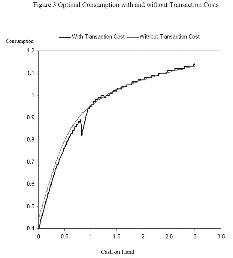
, of two consecutive iterations becomes small enough (![]() 0.0001). We then can compute the consumption and wealth transfer policy function. Figure 3 is a typical consumption function, projected onto the hyperplane
0.0001). We then can compute the consumption and wealth transfer policy function. Figure 3 is a typical consumption function, projected onto the hyperplane ![]() , which is
equal to half of the mean of quarterly income. The most striking feature of the consumption function is that it is neither continuous nor monotonic. For comparison, I plot a consumption function of the model with no transaction cost in the same figure. We can see that consumption monotonically
increases from slightly higher than 0.4 when
, which is
equal to half of the mean of quarterly income. The most striking feature of the consumption function is that it is neither continuous nor monotonic. For comparison, I plot a consumption function of the model with no transaction cost in the same figure. We can see that consumption monotonically
increases from slightly higher than 0.4 when ![]() to 0.895 when
to 0.895 when ![]() . Over this
region, consumption is consistently above cash balances
. Over this
region, consumption is consistently above cash balances ![]() , suggesting that the consumer has paid the transaction cost and has withdrawn money from the asset account. Then there is a sharp
discontinuous decrease of consumption to 0.82. The discontinuous decrease indicates that the consumer has entered the no-wealth-transferring region. Within the left part of the region, when
, suggesting that the consumer has paid the transaction cost and has withdrawn money from the asset account. Then there is a sharp
discontinuous decrease of consumption to 0.82. The discontinuous decrease indicates that the consumer has entered the no-wealth-transferring region. Within the left part of the region, when ![]() increases from 0.82 to 0.94, consumption increases at a one-for-one rate with
increases from 0.82 to 0.94, consumption increases at a one-for-one rate with ![]() . This region is where the consumer is cash constrained and has MPC=1. Although staying cash
constrained violates the Euler equation, within this region the utility loss from imperfect intertemporal substitution is smaller than the utility loss from the income reduction due to payments of the transaction cost. When
. This region is where the consumer is cash constrained and has MPC=1. Although staying cash
constrained violates the Euler equation, within this region the utility loss from imperfect intertemporal substitution is smaller than the utility loss from the income reduction due to payments of the transaction cost. When ![]() increases above 0.94, the consumer is no longer cash constrained. However, the cash left after paying for consumption is insufficient for the consumer to be willing to pay the transaction cost and transfer the cash left into the asset account. Notice that the
slope of the consumption function with transaction cost is steeper than the one with no transaction cost, for the reasons discussed before. There is another discrete decrease when
increases above 0.94, the consumer is no longer cash constrained. However, the cash left after paying for consumption is insufficient for the consumer to be willing to pay the transaction cost and transfer the cash left into the asset account. Notice that the
slope of the consumption function with transaction cost is steeper than the one with no transaction cost, for the reasons discussed before. There is another discrete decrease when ![]() increases to above 1.25. At this point, consumption is 1.005. Cash left after paying for consumption is 0.245. The interest the consumer can get if the extra cash is saved is 0.0037, which is smaller than the transaction cost paid. Why does the consumer still want to pay the transaction cost?
Recall the FOC equations (15) and (16). The intertemporal preference when the consumer does not pay the transaction cost is different from the one when the consumer does pay it. The consumer still wants to make the transfer - even when the gain from interest does not compensate for the transaction
cost - because the consumer can now set consumption according to a new intertemporal preference that will lead to higher lifetime utility. In other words, in this situation the intertemporal substitution effect dominates the income effect at the current cash balances.
increases to above 1.25. At this point, consumption is 1.005. Cash left after paying for consumption is 0.245. The interest the consumer can get if the extra cash is saved is 0.0037, which is smaller than the transaction cost paid. Why does the consumer still want to pay the transaction cost?
Recall the FOC equations (15) and (16). The intertemporal preference when the consumer does not pay the transaction cost is different from the one when the consumer does pay it. The consumer still wants to make the transfer - even when the gain from interest does not compensate for the transaction
cost - because the consumer can now set consumption according to a new intertemporal preference that will lead to higher lifetime utility. In other words, in this situation the intertemporal substitution effect dominates the income effect at the current cash balances.
Figure 4 illustrates the optimal level of ![]() as a function of
as a function of ![]() when the
consumer chooses to pay the transaction cost. If we ignore the very low levels of
when the
consumer chooses to pay the transaction cost. If we ignore the very low levels of ![]() , we find that for low
, we find that for low ![]() ,
, ![]() is zero.
is zero. ![]() starts to increase
with
starts to increase
with ![]() when
when ![]() is greater than 0.625. Notice that
is greater than 0.625. Notice that ![]() increases at a slower rate than
increases at a slower rate than ![]() does. The figure shows that
does. The figure shows that ![]() is a concave function of
is a concave function of ![]() .9
.9
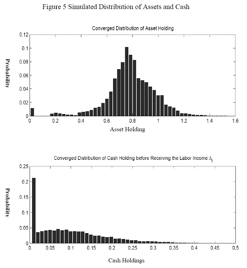
5.1 Simulated Assets and Cash Distribution
The next step is to compute the stationary distribution of the state variables ![]() and
and ![]() because I want to compute the cross section average MPC based upon such a distribution. Clarida (1987) proves that the distribution of asset holding will converge to some steady-state distribution in an economy in which assets are the only state variable. I cannot prove that result
for an economy in which there is more than one state variable. However, simulation results show that the distributions of
because I want to compute the cross section average MPC based upon such a distribution. Clarida (1987) proves that the distribution of asset holding will converge to some steady-state distribution in an economy in which assets are the only state variable. I cannot prove that result
for an economy in which there is more than one state variable. However, simulation results show that the distributions of ![]() and
and ![]() indeed become stationary after a few rounds of iteration starting with any reasonable distributions of
indeed become stationary after a few rounds of iteration starting with any reasonable distributions of ![]() and
and ![]() . The top panel of figure 5 shows the histogram of the converged distribution of asset holdings. The bottom panel shows the converged distribution of cash holdings before receipt of labor income. Table 3 summarizes the
characteristics of the converged assets, cash, and wealth distribution of the baseline parameterization. The mean of the asset distribution is about 80 percent of the mean of quarterly income, and the standard deviation is around 0.2, which is larger than the dispersion of the income distribution.
The distribution of
. The top panel of figure 5 shows the histogram of the converged distribution of asset holdings. The bottom panel shows the converged distribution of cash holdings before receipt of labor income. Table 3 summarizes the
characteristics of the converged assets, cash, and wealth distribution of the baseline parameterization. The mean of the asset distribution is about 80 percent of the mean of quarterly income, and the standard deviation is around 0.2, which is larger than the dispersion of the income distribution.
The distribution of ![]() has a large spike at
has a large spike at ![]() . The spike suggests that more
than 20 percent of consumers either have been cash constrained or have paid the transaction cost and have chosen to carry no cash into the next period. The mean of the cash holdings distribution is 0.1, and the standard deviation is 0.09. The demand for cash has two component - one is active and
the other is passive. The active demand for cash is based on precautionary motivation, as discussed before. The passive demand for cash comes from the consumers who have
. The spike suggests that more
than 20 percent of consumers either have been cash constrained or have paid the transaction cost and have chosen to carry no cash into the next period. The mean of the cash holdings distribution is 0.1, and the standard deviation is 0.09. The demand for cash has two component - one is active and
the other is passive. The active demand for cash is based on precautionary motivation, as discussed before. The passive demand for cash comes from the consumers who have ![]() but have
chosen not to pay the transaction cost. They simply carry the residual cash,
but have
chosen not to pay the transaction cost. They simply carry the residual cash, ![]() , into the next period. Finally, the probability of paying the transaction costs is about 9 percent.
, into the next period. Finally, the probability of paying the transaction costs is about 9 percent.
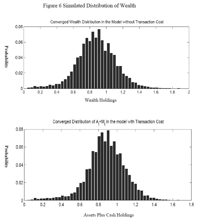
To compare our results with the model with no transaction costs, I plot the histogram of the stationary wealth distribution of the model without transaction costs as in Carroll(1997) (upper panel of figure 6). It is well approximated by a normal distribution. The mean of wealth distribution is
about 0.88, and the standard deviation is 0.23. The counterpart for wealth in our model with transaction costs is ![]() . I plot the histogram of
. I plot the histogram of ![]() in the lower panel of figure 6. Although neither
in the lower panel of figure 6. Although neither ![]() nor
nor ![]() have a normal distribution,
have a normal distribution, ![]() is similar to a normal distribution. The mean of
is similar to a normal distribution. The mean of ![]() is 0.89, and the standard deviation is 0.21. These values suggest that the overall saving behavior has not been changed substantially by the transaction cost.
is 0.89, and the standard deviation is 0.21. These values suggest that the overall saving behavior has not been changed substantially by the transaction cost.
5.2 Simulated Average MPC from Unanticipated Shocks
Now we can compute the MPC for windfall shocks of various sizes. As mentioned earlier, if the population asset and cash holdings are distributed as the converged distribution, the probability of having to pay a transaction cost is about 9 percent. I simulated 20,000 households using the
converged distribution of ![]() and
and ![]() . The top two rows of table 4 summarizes the
consumption response to various income changes. I compute the average MPC for a shock equal to 5 percent of the mean of quarterly income and the average MPC for a shock equal to 50 percent of the mean of quarterly income. I refer to the model without transaction cost as the standard model. As table
4 shows, in the standard model, for the 5 percent shock (small shock), MPC = 0.13; for the 50 percent shock (big shock), MPC = 0.10. The diminishing MPC in the standard model comes from the concavity of the consumption function, as Carroll and Kimball (1996) have pointed out. However, the MPC is
still substantially lower than the estimates of Bodkin(1959) and Hall and Mishkin(1982). In the model with transaction costs, a 5 percent (small) income shock induces an MPC = 0.23, which is 10 percent larger than the MPC in standard model and is close to the estimate by Hall and Mishkin (1982).
For a 50 percent (big) shock, MPC = 0.13, which is still larger than the MPC in the standard model.
. The top two rows of table 4 summarizes the
consumption response to various income changes. I compute the average MPC for a shock equal to 5 percent of the mean of quarterly income and the average MPC for a shock equal to 50 percent of the mean of quarterly income. I refer to the model without transaction cost as the standard model. As table
4 shows, in the standard model, for the 5 percent shock (small shock), MPC = 0.13; for the 50 percent shock (big shock), MPC = 0.10. The diminishing MPC in the standard model comes from the concavity of the consumption function, as Carroll and Kimball (1996) have pointed out. However, the MPC is
still substantially lower than the estimates of Bodkin(1959) and Hall and Mishkin(1982). In the model with transaction costs, a 5 percent (small) income shock induces an MPC = 0.23, which is 10 percent larger than the MPC in standard model and is close to the estimate by Hall and Mishkin (1982).
For a 50 percent (big) shock, MPC = 0.13, which is still larger than the MPC in the standard model.
Although the simulated average MPC out of small windfall income in the model with baseline parameters is still substantially lower than that in Bodkin(1959), changing several parameters can cause the MPC to increase. First, inflation will make holding cash more costly, and consumers will want to
increase current consumption by even more than in the baseline model. Second, lower parameters of ![]() will make cash constraint less costly and consumers will be more likely to choose to be
cash constrained and, in turn, have very high MPC. Third, larger transaction costs lead to a wider s-S band and higher average MPC. Later in the paper, I will explore to what extent these alternative parameters help to increase the MPC. Finally, there could be some
aggregated shock that systematically makes a larger subset of the consumers cash constrained. The more consumers are constrained, the higher the average MPC will be.
will make cash constraint less costly and consumers will be more likely to choose to be
cash constrained and, in turn, have very high MPC. Third, larger transaction costs lead to a wider s-S band and higher average MPC. Later in the paper, I will explore to what extent these alternative parameters help to increase the MPC. Finally, there could be some
aggregated shock that systematically makes a larger subset of the consumers cash constrained. The more consumers are constrained, the higher the average MPC will be.
5.3 Simulated Average Consumption Growth in Response to Anticipated Shocks
To understand why people are sometimes excessively sensitive to anticipated income shocks, we consider the following problem. Suppose at time ![]() , the consumer gets the news that next
period's income will increase by
, the consumer gets the news that next
period's income will increase by
![]() . By how much should today's consumption increase? Furthermore, if an econometrician tests the orthogonality condition by regressing
. By how much should today's consumption increase? Furthermore, if an econometrician tests the orthogonality condition by regressing
![]() on
on
![]() , under what circumstance would he get a positive coefficient? Would the standard model and the model of transaction costs provide different results? To pin down the optimal
consumption in time
, under what circumstance would he get a positive coefficient? Would the standard model and the model of transaction costs provide different results? To pin down the optimal
consumption in time ![]() , given that future income will increase by
, given that future income will increase by
![]() , the consumer solves
, the consumer solves
| (19) |
subject to equation (2.7), and
 |
(20) |
The only difference between equation (21) and equation (6) is that I changed
![]()
![]() to
to
![]() , where
, where ![]() is defined in equation (22)
as the real cash balance carried from period
is defined in equation (22)
as the real cash balance carried from period ![]() plus the anticipated income change
plus the anticipated income change
![]() . In period
. In period ![]() , the consumer will solve the regular optimization
problem (equation 11, 12, and 13) again. Using the computed expected value function,
, the consumer will solve the regular optimization
problem (equation 11, 12, and 13) again. Using the computed expected value function,
![]() , we can compute the optimal
, we can compute the optimal ![]() and
and
![]() . We also compute the optimal
. We also compute the optimal ![]() and
and ![]() for the standard model with no transaction cost.
for the standard model with no transaction cost.
The bottom two rows of table 4 report the response of consumption to small (5 percent) and big (50 percent) anticipated income shocks in a model with and without transaction costs. We find that for both small and big income shocks, the standard model that has no transaction costs predicts the
average of
![]() . This prediction is consistent with the PIH because the consumer in the model is assumed to be impatient, in the sense that
. This prediction is consistent with the PIH because the consumer in the model is assumed to be impatient, in the sense that ![]() . The model with transaction costs predicts that for small anticipated changes in income, the cross section average of
. The model with transaction costs predicts that for small anticipated changes in income, the cross section average of
![]() is larger than zero. This fact suggests excess sensitivity to anticipated income change. For large income changes, the cross section average of
is larger than zero. This fact suggests excess sensitivity to anticipated income change. For large income changes, the cross section average of
![]() is negative and suggests no or very little excess sensitivity. The results are further evidence that people respond to small anticipated income shocks more than the
theory predicted.
is negative and suggests no or very little excess sensitivity. The results are further evidence that people respond to small anticipated income shocks more than the
theory predicted.
Why does the consumer respond only to small anticipated shocks with excess sensitivity? The reason for consumption smoothing is found in the concavity of the utility function and intertemporal substitution. With transaction costs and a gain from consumption smoothing that is not as large as the utility loss from the payment of a transaction cost, the consumer will not adjust consumption immediately after the arrival of the news of the shock. The consumer will be better off if she waits until the receipt of the income.
5.4 Simulation Results for Alternative Parameters
The above exercises have been repeated for various alternations of the baseline parameters. Table 5 extends table 3 and table 6 extends table 4 to show the effects of parameter alternations.
First, I change the magnitude of the transaction costs. I try both a smaller and a larger transaction cost than in the baseline model. In table 5, under the column of
![]() , the transaction costs are set equal to 0.5 percent of the mean of quarterly income, half of the baseline magnitude. Not surprisingly, because of a lower transaction cost, the
consumer no longer worries about having to pay the costs as much as in the baseline model. This lack of concern is reflected in a lower mean of the distribution of cash holdings over periods: compared with the baseline model, the mean of cash holdings decreases from 0.1 to 0.07. This decrease in
cash holding is partly offset in an increase in asset holdings, the mean of which increases from 0.80 to 0.82. Consequently, total wealth saved decreased slightly relative to the baseline case. Because of the smaller transaction cost, the s-S band is narrower, and the
contraction implies that the consumer pays the cost more often (the probability of paying the transaction cost increases to 18.8 percent), and the induced MPC out of both small and big unanticipated income shock is smaller than in the baseline case. As shown in table 6 under the column of
, the transaction costs are set equal to 0.5 percent of the mean of quarterly income, half of the baseline magnitude. Not surprisingly, because of a lower transaction cost, the
consumer no longer worries about having to pay the costs as much as in the baseline model. This lack of concern is reflected in a lower mean of the distribution of cash holdings over periods: compared with the baseline model, the mean of cash holdings decreases from 0.1 to 0.07. This decrease in
cash holding is partly offset in an increase in asset holdings, the mean of which increases from 0.80 to 0.82. Consequently, total wealth saved decreased slightly relative to the baseline case. Because of the smaller transaction cost, the s-S band is narrower, and the
contraction implies that the consumer pays the cost more often (the probability of paying the transaction cost increases to 18.8 percent), and the induced MPC out of both small and big unanticipated income shock is smaller than in the baseline case. As shown in table 6 under the column of
![]() , the MPC for the 5 percent (small) income shock is 0.202, decreasing from 0.236 in the baseline model, and for the 50 percent (big) income shock, the MPC is 0.117, comparing
with 0.132 in the baseline model. We can see that the MPC is still larger than in the case in which there are no transaction costs (standard model in table 4). In addition, the model still implies an excess sensitivity in response to anticipated income shocks when the shocks are small (in this case
, the MPC for the 5 percent (small) income shock is 0.202, decreasing from 0.236 in the baseline model, and for the 50 percent (big) income shock, the MPC is 0.117, comparing
with 0.132 in the baseline model. We can see that the MPC is still larger than in the case in which there are no transaction costs (standard model in table 4). In addition, the model still implies an excess sensitivity in response to anticipated income shocks when the shocks are small (in this case
![]() , greater than zero).
, greater than zero).
For larger transaction costs (![]() equal to 2 percent of mean income) the findings are more economically significant than in the baseline case. As we can we see in table 5, under the
column of
equal to 2 percent of mean income) the findings are more economically significant than in the baseline case. As we can we see in table 5, under the
column of
![]() , the mean of the precautionary cash holding increases to 0.12, and the mean of total saving increases to 0.92. In table 6 the corresponding column suggests that the increased
transaction cost also significantly increased MPC out of both small and big unanticipated income shocks, to 0.249 and 0.168, respectively, because of the wider s-S band (the probability of people paying the transaction cost is only 7.7 percent). For anticipated income
changes, we get excess sensitivity for both 5 and 50 percent anticipated changes in income, that is
, the mean of the precautionary cash holding increases to 0.12, and the mean of total saving increases to 0.92. In table 6 the corresponding column suggests that the increased
transaction cost also significantly increased MPC out of both small and big unanticipated income shocks, to 0.249 and 0.168, respectively, because of the wider s-S band (the probability of people paying the transaction cost is only 7.7 percent). For anticipated income
changes, we get excess sensitivity for both 5 and 50 percent anticipated changes in income, that is
![]() . However, when the size of the anticipated income change is increased to 100 percent of the mean of quarterly labor income, not shown in the table, the excess sensitivity
fades out.
. However, when the size of the anticipated income change is increased to 100 percent of the mean of quarterly labor income, not shown in the table, the excess sensitivity
fades out.
I then study the effects of adding inflation to the model. I consider both mild inflation and high inflation. The results are show in table 5 and table 6 under the column of
![]() and
and
![]() . Inflation makes holding cash more costly, so if the consumer decides not to pay the transaction cost, the MPC out of cash will be higher. This result is shown in the Euler
equation(15). Higher
. Inflation makes holding cash more costly, so if the consumer decides not to pay the transaction cost, the MPC out of cash will be higher. This result is shown in the Euler
equation(15). Higher ![]() will reduce the current period's marginal utility and increase future marginal utility; therefore, consumption growth decreases. However, because holding cash costs
more, the s-S is narrower (the probability of paying a transaction cost is as high as 23.7 percent), and people pay the transaction costs more frequently. The overall effect of inflation is ambiguous without seeing the numerical results.
will reduce the current period's marginal utility and increase future marginal utility; therefore, consumption growth decreases. However, because holding cash costs
more, the s-S is narrower (the probability of paying a transaction cost is as high as 23.7 percent), and people pay the transaction costs more frequently. The overall effect of inflation is ambiguous without seeing the numerical results.
Simulation results suggest that the higher probability of paying the transaction cost is offset by the increase in MPC within the s-S band. When
![]() , the MPC is 0.257 for small income shocks and 0.123 for large income shocks. When
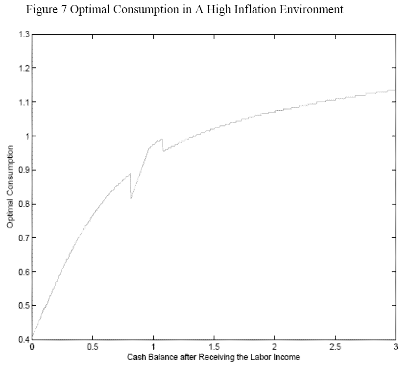
, the MPC is 0.257 for small income shocks and 0.123 for large income shocks. When ![]() , the MPC becomes 0.304 and 0.121 for small shocks and large shocks, respectively. Figure 7 shows the optimal consumption as a function of cash holdings after receiving the labor income for a given level of
, the MPC becomes 0.304 and 0.121 for small shocks and large shocks, respectively. Figure 7 shows the optimal consumption as a function of cash holdings after receiving the labor income for a given level of ![]() =0.5. When we compare figure 7 with figure 3, we see that the s-S band in figure 7 is narrower; but that within the band, more people are in the MPC=1 region in Figure 7. Money thus burns a hole in the high inflation
episodes if people hold cash. The pattern of excess sensitivity for anticipated income is similar to that in the baseline model.
=0.5. When we compare figure 7 with figure 3, we see that the s-S band in figure 7 is narrower; but that within the band, more people are in the MPC=1 region in Figure 7. Money thus burns a hole in the high inflation
episodes if people hold cash. The pattern of excess sensitivity for anticipated income is similar to that in the baseline model.
Finally, I show how different intertemporal elasticities of substitution (IES) would affect the results. I consider the case of log preference (![]() ) and
) and ![]() . The results are presented in table 5 and table 6 under the columns of
. The results are presented in table 5 and table 6 under the columns of ![]() and
and ![]() , respectively. Lower
, respectively. Lower ![]() yields a higher IES which makes consumers more willing to
substitute consumption between periods. For a high IES, we find significantly lower wealth accumulation as the consumer has a weaker precautionary motivation to save. This finding is consistent with Carroll (1997). The consumer also has a weaker precautionary demand for cash. The mean demand for
cash is only 6.6 percent of mean labor income. The consumer does not care that much about intertemporal substitution or being cash-constrained. Therefore, the probability of paying the transaction cost is low (0.645). The MPC from unanticipated shocks is very high, and excess sensitivity to
anticipated income shocks is robust even for very large shocks. In the case of a low IES, we have the opposite results. Specifically, wealth accumulation is very high, the MPC from an unanticipated income shock is low, and the excess sensitivity in response to an anticipated income shock cannot be
detected even for small income shocks.
yields a higher IES which makes consumers more willing to
substitute consumption between periods. For a high IES, we find significantly lower wealth accumulation as the consumer has a weaker precautionary motivation to save. This finding is consistent with Carroll (1997). The consumer also has a weaker precautionary demand for cash. The mean demand for
cash is only 6.6 percent of mean labor income. The consumer does not care that much about intertemporal substitution or being cash-constrained. Therefore, the probability of paying the transaction cost is low (0.645). The MPC from unanticipated shocks is very high, and excess sensitivity to
anticipated income shocks is robust even for very large shocks. In the case of a low IES, we have the opposite results. Specifically, wealth accumulation is very high, the MPC from an unanticipated income shock is low, and the excess sensitivity in response to an anticipated income shock cannot be
detected even for small income shocks.
6 On the Equity Premium Puzzle
Assume the CRRA type of utility functions. The standard consumption-based capital asset pricing model (C-CAPM) leads to the following well-known relationship
![\displaystyle E_t\left[\beta\left(\frac{C_{t+1}}{C_t}\right)^\rho (1 + r_t) - 1 \right] = 0.](img152.gif)
Tests of the theory will typically use macro data to fit equation (21) with
The estimated high value of
![]() can be consistent with a low actual level of
can be consistent with a low actual level of ![]() estimated from other
approaches with various extensions to the model. Gabaix and Laibson (2001) pointed out that if consumers adjust their consumption plan only infrequently, say, every
estimated from other
approaches with various extensions to the model. Gabaix and Laibson (2001) pointed out that if consumers adjust their consumption plan only infrequently, say, every ![]() periods, and aggregated
consumption growth is then used to fit equation (23), the estimated
periods, and aggregated
consumption growth is then used to fit equation (23), the estimated
![]() can be upward biased by a factor of up to 6
can be upward biased by a factor of up to 6![]() . They call this effect
the
. They call this effect
the ![]() bias. Reis (2006) assumed that the consumers get information infrequently, and during the time that they are not updating their information they are "inattentive." His model also
predicts an upward bias to
bias. Reis (2006) assumed that the consumers get information infrequently, and during the time that they are not updating their information they are "inattentive." His model also
predicts an upward bias to
![]() .
.
In a similar spirit, I extend the model in Section 3 to allow for labor income risks as well as asset return risks. This model is state dependent, and does not rely on assumptions like infrequent update of information. The model, however, can lead to results that are related to those in Gabaix
and Laibson(2001) and Reis(2006). The real return on assets is assumed to follow some stochastic process and ![]() is observed after the consumer has made decisions on
is observed after the consumer has made decisions on
![]() . Therefore, the realization of
. Therefore, the realization of ![]() has an effect on
decisions made only in period
has an effect on
decisions made only in period ![]() and later. Mechanically, in the model equation (6) to (14), the only equation that needs modification is equation (7). If we take into account the stochastic
asset return, the motion equation of state variable
and later. Mechanically, in the model equation (6) to (14), the only equation that needs modification is equation (7). If we take into account the stochastic
asset return, the motion equation of state variable ![]() is
is
 |
(22) |
The consumer will enter period
Consider a situation in which the consumer holds some ![]() and
and ![]() in period t
- 1 after paying for the consumption expenditure but before
in period t
- 1 after paying for the consumption expenditure but before ![]() is realized. For any realization of
is realized. For any realization of
![]() , there always exists one realization of
, there always exists one realization of ![]() such that
such that
![]() , where
, where ![]() is the optimal
consumption level in an economy where there is no transaction cost. Such a combination of
is the optimal
consumption level in an economy where there is no transaction cost. Such a combination of ![]() and
and ![]() should leave the consumer in a first best situation.
should leave the consumer in a first best situation.
Now imagine that the consumer still receives the same realization,
![]() , but the realized
, but the realized ![]() is only slightly higher than the predicted
is only slightly higher than the predicted
![]() . In an economy without transaction cost, consumption should increase in response to the higher asset return. However, in the current model, the higher consumption is not optimal. The
consumer's current cash holding can accommodate consumption of only
. In an economy without transaction cost, consumption should increase in response to the higher asset return. However, in the current model, the higher consumption is not optimal. The
consumer's current cash holding can accommodate consumption of only
![]() ; beyond that the consumer has to withdraw money from the asset account. When the change in
; beyond that the consumer has to withdraw money from the asset account. When the change in ![]() is not very large, the consumer still consume
is not very large, the consumer still consume
![]() ,and remain fairly close to the first best situation; hence the consumer should not pay the transaction cost. Thus, for a certain range of
,and remain fairly close to the first best situation; hence the consumer should not pay the transaction cost. Thus, for a certain range of ![]() the correlation between consumption growth and
the correlation between consumption growth and ![]() is literally zero for some
given
is literally zero for some
given
![]() . If we compute the average correlation across the distribution of
. If we compute the average correlation across the distribution of ![]() and
and
![]() , the correlation is positive but lower than in the economy without transaction costs.
, the correlation is positive but lower than in the economy without transaction costs.
How important will this effect be quantitatively? The answer depends on how many consumers are on the linear part of the consumption function. Only those consumers who are cash constrained will not vary their consumption with the fluctuations in the equity market. The fraction of
cash-constrained consumers, in turn, depends on the size of transaction cost, ![]() . The larger
. The larger ![]() is, the wider the
is, the wider the ![]() band is, and the more cash-constrained consumers there are. However, for the magnitude of the transaction cost assumed in this paper, or any value
close to that, this model cannot reduce the correlation between consumption growth and asset returns to a level that is consistent with a plausible value of
band is, and the more cash-constrained consumers there are. However, for the magnitude of the transaction cost assumed in this paper, or any value
close to that, this model cannot reduce the correlation between consumption growth and asset returns to a level that is consistent with a plausible value of ![]() . Unlike the powerful
. Unlike the powerful
![]() model, which lowers the required
model, which lowers the required ![]() by a factor of 24, the transaction cost
model lowers the required
by a factor of 24, the transaction cost
model lowers the required ![]() only mildly. Conversely, the value of
only mildly. Conversely, the value of ![]() that can
lower
that can
lower ![]() to the neighborhood of 4 or 5 is unrealistically large.
to the neighborhood of 4 or 5 is unrealistically large.
It is well known that the equity premium puzzle is very hard to be resolved by the introduction of one new assumption. The transaction cost model may help explain the puzzle better when the model is integrated with other assumptions that have been partly successful in explaining the equity premium puzzle.
7 Conclusion
In this paper, I construct a model with transaction costs in a cash-in-advance economy. The model helps to explain the observation that the MPC out of small unanticipated income shocks is in general higher than the MPC out of large such shocks. It also helps explain why econometricians find excess sensitivity to anticipated income changes only when the changes are relatively small. These results do not rely on assumptions about liquidity constraints or any other behavioral assumptions. Furthermore, the model predicts a demand for cash, or in a broader sense, a demand for liquid assets that arises from a precautionary motivation. Finally, an extension of the model serves as a state-dependent paradigm of how consumption responds to stochastic asset returns, and can help to solve the equity premium puzzle.
Two caveats apply to the current model. First, the income process adopted in this model is primitive. To make the computation less expensive, I did not allow for any persistent income process or income growth. Also, the model is partial equilibrium. For shocks at the aggregate level, general equilibrium effects will need to be taken into account.
The magnitude of the transaction cost plays an important role in determining the s-S band width. Therefore, future research is needed to uncover solid empirical estimates of the magnitude. Recent developments in the research of limited participation in the equity market provide some estimates of the magnitude of related frictions. For example, Vissing-Jørgensen (2002) estimates that a per-period stock market participation cost of just 50 dollars is sufficient to explain the choices of half of stock market nonparticipants.
The simulated results of the model have also yielded some testable implications such as that the MPC from windfall income is higher when inflation is high, and that the correlation between asset return and consumption growth is higher when labor income is more volatile. Future research will seek to verify these implications.
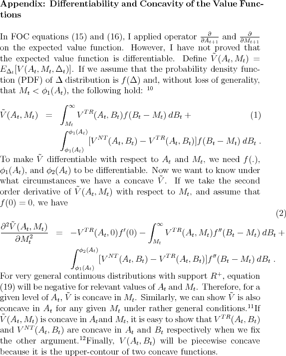
| Type of Income Change, Study | Experiments and Data Sources | Big Change or Small Change | Findings |
|---|---|---|---|
| Unanticipated Change: Bodkin(1959) | National Service Life Insurance payments | Small change | MPC between 0.7 and 0.9 |
| Unanticipated Change: Bodkin(1966) | National Service Life Insurance payments | Small change | Cannot reject the relationship between the size of windfall income shock and MPC |
| Anticipated Change: Flavin(1981) | Macro data | N/A | Excess sensitivity detected |
| Anticipated Change: Hall (1982) | Macro data | N/A | Excess sensitivity detected |
| Unanticipated Change: Hall and Mishkin(1982) | PSID data | N/A | MPC around 0.29 |
| Anticipated Change: Hsieh(2003) | Alaska Oil Revenue Fund payments in CEX | Big change | Excess sensitivity not detected |
| Unanticipated Change: Kreinin(1961) | Reparations payments to Israelis | Big change | MPC around 0.16 |
| Unanticipated Change: Landsberger(1966) | Reparations payments to Israelis | Small and big change | Strong evidence of decreasing MPC when |
| windfall income becomes larger | |||
| Anticipated Change: Parker(1999) | Tax withholding changes in CEX | Small change | Excess sensitivity detected |
| Liquidity Constraints: Parker(1999) | Tax withholding changes in CEX data | Does not support the model | |
| Liquidity Constraints: Runkle(1991) | PSID data | Does not support the model | |
| Liquidity Constraints: Shapiro and Slemrod(2003) | Survey data | Does not support the model | |
| Anticipated Change: Souleles(1999) | Tax refund in CEX | Small change | Excess sensitivity detected |
| Liquidity Constraints: Souleles(1999) | Tax refund in CEX Data | Supports the liquidity constraints model | |
| Anticipated Change: Souleles(2001) | College tuition payments in CEX | Big change | Excess sensitivity not detected |
| Anticipated Change: Souleles(2002) | Phase two Reagan tax cuts in CEX | Small change | Excess sensitivity detected |
| Liquidity Constraints: Souleles(2002) | Phase two Reagan tax cuts in CEX data | Does not support the model | |
| Liquidity Constraints: Zeldes(1989a) | PSID data | Supports the liquidity constraints model |
| real interest rate |
0.015 |
|---|---|
| discount rate |
0.025 |
| prob of very low income |
0.01 |
| transaction cost |
0.01 |
| mean of income
|
1 |
| standard deviation of income
|
0.1 |
| risk aversion coefficient |
2 |
| inflation rate |
0 |
| Mean (SD) of the Converged Asset Distribution | 0.79 (0.19) |
|---|---|
| Mean (SD) of the Converged Cash Distribution | 0.10 (0.09) |
| Mean (SD) of the Converged Wealth Distribution | 0.89 (0.21) |
| Probability of Paying the Transaction Costs | 8.8% |
Notes: The mean and standard deviation is relative to the mean of income.
| Income Change | Standard Model | Benchmark Model |
|---|---|---|
| Unanticipated: Small (5%) income shock | 0.135 | 0.236 |
| Unanticipated: Big (50%) income shock | 0.109 | 0.132 |
| Anticipated: Small (5%) income shock | -0.0017 | 0.0015 |
| Anticipated: Big (50%) income shock | -0.0035 | -0.0011 |
Notes: The standard model refers to the model with no transaction costs, the benchmark model refers to the model with transaction costs, both with parameters defined in table 2.
| Value | y = 0.005 | y = 0.02 | p = 0.01 | p = 0.05 | r = 1 | r = 7 |
|---|---|---|---|---|---|---|
| Mean (SD) of the converged assets distribution | 0.819 (0.208) | 0.795 (0.207) | 0.836 (0.201) | 0.899 (0.220) | 0.525 (0.168) | 2.119 (0.363) |
| Mean (SD) of the converged cash distribution | 0.068 (0.066) | 0.121 (0.103) | 0.067 (0.066) | 0.022 (0.030) | 0.065 (0.068) | 0.136 (0.098) |
| Mean (SD) of the converged wealth distribution | 0.886 (0.221) | 0.916 (0.211) | 0.903 (0.212) | 0.920 (0.222) | 0.590 (0.172) | 2.254 (0.380) |
| Probability of paying the transaction costs | 0.1875 | 0.0774 | 0.134 | 0.2371 | 0.0645 | 0.3666 |
Notes: The mean and standard deviation is relative to the mean of income.
| Income Change | y = 0.005 | y = 0.02 | p = 0.01 | p = 0.05 | r = 1 Log(C) | r = 7 |
|---|---|---|---|---|---|---|
| Unanticipated: Small (5%) income shock | 0.202 | 0.249 | 0.257 | 0.304 | 0.372 | 0.078 |
| Unanticipated: Big (50%) income shock | 0.117 | 0.168 | 0.123 | 0.121 | 0.209 | 0.068 |
| Anticipated: Small (5%) income shock | 0.0009 | 0.0028 | 0.0022 | 0.0057 | 0.014 | -0.053 |
| Anticipated: Big (50%) income shock | -0.0051 | 0.016 | -0.0042 | -0.0064 | 0.053 | -0.121 |