
Combining Forecasts From Nested Models *
Keywords: Forecast combination, predictability, forecast evaluation
Abstract:
JEL Nos.: C53, C52
1 Introduction
Forecasters are well aware of the so-called principle of parsimony: "simple, parsimonious models tend to be best for out-of-sample forecasting..." (Diebold (1998)). Although an emphasis on parsimony may be justified on various grounds, parameter estimation error is one key reason. In many practical situations, estimating additional parameters can raise the forecast error variance above what might be obtained with a simple model. Such is clearly true when the additional parameters have population values of zero. But the same can apply even when the population values of the additional parameters are non-zero, if the marginal explanatory power associated with the additional parameters is low enough. In such cases, in finite samples the additional parameter estimation noise may raise the forecast error variance more than including information from additional variables lowers it. For example, simulation evidence in Clark and McCracken (2006) shows that even though the true model relates inflation to the output gap, in finite samples a simple AR model for inflation will often forecast as well as or better than the true model.1
As this discussion suggests, parameter estimation noise creates a forecast accuracy tradeoff. Excluding variables that truly belong in the model could adversely affect forecast accuracy. Yet including the variables could raise the forecast error variance if the associated parameters are estimated sufficiently imprecisely. In light of such a tradeoff, combining forecasts from the unrestricted and restricted (or parsimonious) models could improve forecast accuracy. Such combination could be seen as a form of shrinkage, which various studies, such as Stock and Watson (2003), have found to be effective in forecasting.
Accordingly, this paper presents analytical, Monte Carlo, and empirical evidence on the effectiveness of combining forecasts from nested models. Our analytics are based on models we characterize as "weakly" nested: the unrestricted model is the true model, but as the sample size grows large, the data generating process (DGP) converges to the restricted model. This analytic approach captures the practical reality that the predictive content of some variables of interest is often quite low. Although we focus the presented analysis on nested linear models, our results could be generalized to nested nonlinear models.
Under the weak nesting specification, we derive weights for combining the forecasts from estimates of the restricted and unrestricted models that are optimal in the sense of minimizing the forecast mean square error (MSE). We then characterize the settings under which the combination forecast will be better than the restricted or unrestricted forecasts. In the special case in which the coefficients on the extra variables in the unrestricted model are of a magnitude that makes the restricted and unrestricted models equally accurate, the MSE-minimizing forecast is a simple, equally-weighted average of the restricted and unrestricted forecasts.
In the Monte Carlo and empirical analysis, we show our proposed approach of combining forecasts from nested models to be effective for improving accuracy. To ensure the practical relevance of our results, we base our Monte Carlo experiments on DGPs calibrated to empirical applications, and, in our empirical work, we consider a range of applications. In the applications, our proposed combination approaches work well compared to related alternatives, consisting of Bayesian-type estimation with priors that push certain coefficients toward zero and Bayesian model averaging of the restricted and unrestricted models.
Our results build on much prior work on forecast combination. Research focused on non-nested models ranges from the early work of Bates and Granger (1969) to recent contributions such as Stock and Watson (2003) and Elliott and Timmermann (2004).2 Combination of nested model forecasts has been considered only occasionally, in such studies as Goyal and Welch (2003) and Hendry and Clements (2004). Forecasts based on Bayesian model averaging as applied in such studies as Wright (2003) and Jacobson and Karlsson (2004) could also combine forecasts from nested models. Of course, such Bayesian methods of combination are predicated on model uncertainty. In contrast, our paper provides a theoretical rationale for nested model combination in the absence of model uncertainty.
The paper proceeds as follows. Section 2 provides theoretical results on the possible gains from combination of forecasts from nested models, including the optimal combination weight. In section 3 we present Monte Carlo evidence on the finite sample effectiveness of our proposed forecast combination methods. Section 4 compares the effectiveness of the forecast methods in a range of empirical applications. Section 5 concludes. Additional theoretical details are presented in Appendix 1.
2 Theory
We begin by using a simple example to illustrate our essential ideas and results. We then proceed to the more general case. After detailing the necessary notation and assumptions, we provide an analytical characterization of the bias-variance tradeoff, created by weak predictability, involved in choosing among restricted, unrestricted, and combined forecasts. In light of that tradeoff, we then derive the optimal combination weights.
2.1 A simple example
Suppose we are interested in forecasting ![]() using a simple model relating
using a simple model relating ![]() to a constant and a strictly exogenous, scalar variable
to a constant and a strictly exogenous, scalar variable ![]() . Suppose, however, that the predictive content of
. Suppose, however, that the predictive content of ![]() for
for ![]() may be weak. To capture this possibility, we model the population relationship between
may be weak. To capture this possibility, we model the population relationship between ![]() and
and ![]() using local-to-zero asymptotics, such that, as the sample size grows large, the predictive
content of
using local-to-zero asymptotics, such that, as the sample size grows large, the predictive
content of ![]() shrinks to zero (assume that, apart from the local element, the model fits in the framework of the usual classical normal regression model, with homoskedastic errors,
etc.):
shrinks to zero (assume that, apart from the local element, the model fits in the framework of the usual classical normal regression model, with homoskedastic errors,
etc.):
In light of ![]() 's weak predictive content, the forecast from an estimated model relating
's weak predictive content, the forecast from an estimated model relating ![]() to a constant and
to a constant and ![]() (henceforth, the unrestricted model) could be less accurate than a forecast from a model relating
(henceforth, the unrestricted model) could be less accurate than a forecast from a model relating ![]() to just a constant (the restricted model). Whether that is so depends on the "signal" and "noise" associated with
to just a constant (the restricted model). Whether that is so depends on the "signal" and "noise" associated with ![]() and its estimated coefficient. Under the local asymptotics incorporated in the DGP (1), the signal-to-noise ratio is proportional to
and its estimated coefficient. Under the local asymptotics incorporated in the DGP (1), the signal-to-noise ratio is proportional to
![]() . Given
. Given
![]() and
and
![]() (or
(or ![]() ), higher values of the coefficient on
), higher values of the coefficient on ![]() (or the variance of
(or the variance of ![]() ) raise the signal relative to the noise; given the other parameters, a
higher residual variance
) raise the signal relative to the noise; given the other parameters, a
higher residual variance
![]() increases the noise, reducing the signal-to-noise ratio.
increases the noise, reducing the signal-to-noise ratio.
In light of the tradeoff considerations described in the introduction, a combination of the unrestricted and restricted model forecasts could be more accurate than either of the individual forecasts. We consider a combined forecast that puts a weight of
![]() on the restricted model forecast and
on the restricted model forecast and
![]() on the unrestricted model forecast. We then analytically determine the weight
on the unrestricted model forecast. We then analytically determine the weight
![]() that yields the forecast with lowest expected squared error in period
that yields the forecast with lowest expected squared error in period ![]() .
.
As we establish more formally below, the (estimated) MSE-minimizing combination weight
![]() is a function of the signal-to-noise ratio:
is a function of the signal-to-noise ratio:
![\displaystyle \hat{\alpha}_{t}^{\ast}=\left[ 1+\left( {\frac{{\left( \sqrt{t}\ \hat {b}_{1}\right) ^{2}\hat{\sigma}_{x}^{2}}}{{\hat{\sigma}^{2}}}}\right) \right] ^{-1},%](img13.gif)
where
2.2 The general case: environment
In the general case, the possibility of weak predictors is modeled using a sequence of linear DGPs of the form (Assumption 1)
| (3) | ||
where
For a fixed value of ![]() , our forecasting agent observes the sequence
, our forecasting agent observes the sequence
![]() sequentially at each forecast origin
sequentially at each forecast origin
![]() . Forecasts of the scalar
. Forecasts of the scalar
![]() ,
, ![]() , are generated using a (
, are generated using a (
![]() vector of covariates
vector of covariates
![]() , linear parametric models
, linear parametric models
![]() ,
, ![]() , and a combination of the two models,
, and a combination of the two models,
![]() . The parameters are estimated using OLS (Assumption 2) and hence
. The parameters are estimated using OLS (Assumption 2) and hence
![]() ,
, ![]() , for the restricted and unrestricted models, respectively. We denote the loss associated with the
, for the restricted and unrestricted models, respectively. We denote the loss associated with the ![]() -step ahead forecast errors as
-step ahead forecast errors as
![]() ,
, ![]() , and
, and
![]() for the restricted, unrestricted, and combined,
respectively.
for the restricted, unrestricted, and combined,
respectively.
The following additional notation will be used. Let
![]() =
=
![]() =
=
![]() ,
,
![]() =
=
![]() , and
, and
![]() for
for ![]() . For
. For
![]() , let
, let
![]() , where
, where
![]() is the upper block-diagonal element of
is the upper block-diagonal element of
![]() defined below. For any (
defined below. For any (
![]() matrix
matrix ![]() with elements
with elements ![]() and column vectors
and column vectors ![]() , let:
, let: ![]() denote the
denote the
![]() vector
vector
![]() ;
; ![]() denote
the max norm; and
denote
the max norm; and ![]() denote the trace. Let
denote the trace. Let
![]() and let
and let
![]() denote weak convergence. Finally, we define a variable selection matrix and a coefficient vector that appears directly in our key combination results:
denote weak convergence. Finally, we define a variable selection matrix and a coefficient vector that appears directly in our key combination results:
![]() and
and
![]() .
.
To derive our general results, we need two more assumptions (in addition to our assumptions (1 and 2) of a DGP with weak predictability and OLS-estimated linear forecasting models).
Assumption 3: (a)
![]() where
where
![]() for all
for all
![]() , (b)
, (b)
![]() = 0 all
= 0 all
![]() , (c)
, (c)
![]() for some
for some ![]() , (d)
, (d)
![]() is a zero mean triangular array satisfying Theorem 3.2
of De Jong and Davidson (2000).
is a zero mean triangular array satisfying Theorem 3.2
of De Jong and Davidson (2000).
Assumption 4: For
![]() , (a)
, (a)
![]() , (b)
, (b)
![]() .
.
Assumption 3 imposes three types of conditions. First, in (a) and (c) we require that the observables, while not necessarily covariance stationary, are asymptotically mean square stationary with finite second moments. We do so in order to allow the observables to have marginal distributions that
vary as the weak predictive ability strengthens along with the sample size but are `well-behaved' enough that, for example, sample averages converge in probability to the appropriate population means. Second, in (b) we impose the restriction that the ![]() -step ahead forecast errors are MA(
-step ahead forecast errors are MA(![]() . We do so in order to emphasize the role that weak predictors have on forecasting
without also introducing other forms of model misspecification. Finally, in (d) we impose the high level assumption that, in particular,
. We do so in order to emphasize the role that weak predictors have on forecasting
without also introducing other forms of model misspecification. Finally, in (d) we impose the high level assumption that, in particular,
![]() satisfies Theorem 3.2 of De Jong and Davidson (2000). By doing so we not only insure (results needed in Appendix 1) that certain weighted partial sums converge weakly to
standard Brownian motion, but also allow ourselves to take advantage of various results pertaining to convergence in distribution to stochastic integrals.
satisfies Theorem 3.2 of De Jong and Davidson (2000). By doing so we not only insure (results needed in Appendix 1) that certain weighted partial sums converge weakly to
standard Brownian motion, but also allow ourselves to take advantage of various results pertaining to convergence in distribution to stochastic integrals.
Our final assumption is unique: we permit the combining weights to change with time. In this way, we allow the forecasting agent to balance the bias-variance tradeoff differently across time as the increasing sample size provides stronger evidence of predictive ability. Finally, we impose the
requirement that
![]() and hence the duration of forecasting is finite but non-trivial.
and hence the duration of forecasting is finite but non-trivial.
2.3 Theoretical results on the tradeoff
Our characterization of the bias-variance tradeoff associated with weak predictability is based on
![]() , the difference in the (normalized) MSEs of the unrestricted and combined forecasts. In Appendix 1, we
provide a general characterization of the tradeoff, in Theorem 1. But in the absence of a closed form solution for the limiting distribution of the loss differential (the distribution provided in Appendix 1), we proceed in this section to focus on the mean of this loss differential.
, the difference in the (normalized) MSEs of the unrestricted and combined forecasts. In Appendix 1, we
provide a general characterization of the tradeoff, in Theorem 1. But in the absence of a closed form solution for the limiting distribution of the loss differential (the distribution provided in Appendix 1), we proceed in this section to focus on the mean of this loss differential.
From the general case proved in Appendix 1, we first establish the expected value of the loss differential, in the following corollary.
This decomposition implies that the bias-variance tradeoff depends on: (1) the duration of forecasting (
![]() , (2) the dimension of the parameter vectors (through the dimension of
, (2) the dimension of the parameter vectors (through the dimension of ![]() ), (3) the magnitude of the predictive ability (as measured by quadratics of
), (3) the magnitude of the predictive ability (as measured by quadratics of ![]() ), (4) the forecast horizon (via
), (4) the forecast horizon (via ![]() , the long-run variance of
, the long-run variance of
![]() ), and (5) the second moments of the predictors (
), and (5) the second moments of the predictors (
![]() .
.
The first term on the right-hand side of the decomposition can be interpreted as the pure "variance" contribution to the mean difference in the unrestricted and combined MSEs. The second term can be interpreted as the pure "bias" contribution. Clearly, when ![]() and thus there is no predictive ability associated with the predictors
and thus there is no predictive ability associated with the predictors
![]() , the expected difference in MSE is positive so long as
, the expected difference in MSE is positive so long as
![]() . Since the goal is to choose
. Since the goal is to choose ![]() so that
so that
![]() is maximized, we immediately reach the intuitive conclusion that we should always forecast using the restricted model and hence set
is maximized, we immediately reach the intuitive conclusion that we should always forecast using the restricted model and hence set
![]() . When
. When
![]() , and hence there is predictive ability associated with the predictors
, and hence there is predictive ability associated with the predictors
![]() , forecast accuracy is maximized by combining the restricted and unrestricted model forecasts. The following corollary provides the optimal combination weight. Note that, to
simplify notation in the presented results, from this point forward we omit the subscript
, forecast accuracy is maximized by combining the restricted and unrestricted model forecasts. The following corollary provides the optimal combination weight. Note that, to
simplify notation in the presented results, from this point forward we omit the subscript ![]() from the predictors, so that, e.g.,
from the predictors, so that, e.g.,
![]() is simply denoted
is simply denoted ![]() .
.
![\displaystyle \alpha^{\ast}(s)=\left[ 1+s\left( {\frac{{\beta}_{22}^{\prime}(Ex_{22,t}% {x}_{22,t}^{\prime}-Ex_{22,t}{x}_{1,t}^{\prime}(Ex_{1,t}{x}_{1,t}^{\prime })^{-1}Ex_{1,t}{x}_{22,t}^{\prime})\beta_{22}}{tr((-JB_{1}{J}^{\prime}% +B_{2})V)}}\right) \right] ^{-1} .%](img97.gif)
The optimal combination weight is derived by maximizing the arguments of the integrals in Corollary 1 that contribute to the average expected mean square differential over the duration of forecasting -- hence our " pointwise optimal" characterization of the weight. In particular, the results of Corollary 2 follow from maximizing
with respect to
As is apparent from the formula in Corollary 2, the combining weight is decreasing in the marginal `signal to noise' ratio
In the special case in which the signal-to-noise ratio equals 1, the optimal combination weight is 1/2. That is, for a given time period ![]() , when
, when
and hence the restricted and unrestricted models are expected to be equally accurate,
A bit more algebra establishes the determinants of the size of the benefits to combination. If we substitute
![]() into (5), we find that
into (5), we find that
![]() takes the easily interpretable form
takes the easily interpretable form

This simplifies even more in the conditionally homoskedastic case, in which
Note, however, that the term
![]() is a function of the local-to-zero
parameters
is a function of the local-to-zero
parameters
![]() . Moreover, note that these optimal combining weights are not presented relative to an environment in which agents are forecasting in `real time'. Therefore, for practical use, we
suggest a transformed formula. Let
. Moreover, note that these optimal combining weights are not presented relative to an environment in which agents are forecasting in `real time'. Therefore, for practical use, we
suggest a transformed formula. Let
![]() and
and ![]() denote estimates of
denote estimates of ![]() and
and ![]() , respectively, based on data through period
, respectively, based on data through period ![]() . If we let
. If we let
![]() denote an estimate of the local-to-zero parameter
denote an estimate of the local-to-zero parameter
![]() and set
and set ![]() , we obtain the following real time estimate of
the pointwise optimal combining weight:4
, we obtain the following real time estimate of
the pointwise optimal combining weight:4
![\displaystyle \hat{\alpha}_{t}^{\ast}=\left[ 1+t\left( {\frac{\hat{{\beta}^{\prime}}% _{22}(t^{-1}\sum_{j=1}^{t-\tau}{x_{22,j}{x}_{22,j}^{\prime}}-(t^{-1}\sum _{j=1}^{t-\tau}{x_{22,j}{x}_{1,j}^{\prime}})\hat{B}_{1}(t^{-1}\sum _{j=1}^{t-\tau}{x_{1,j}{x}_{22,j}^{\prime}}))\hat{\beta}_{22}}{tr((-J\hat {B}_{1}{J}^{\prime}+\hat{B}_{2})\hat{V})}}\right) \right] ^{-1}.%](img121.gif)
In doing so, though, we acknowledge that the parameter estimates are not consistent for the local-to-zero parameters on which our theoretical derivations (Corollary 2) are based. The local-to-zero asymptotics allow us to derive closed-form solutions for the optimal combination weights, but require knowledge of local-to-zero parameters that cannot be estimated consistently. We therefore simply use rescaled OLS magnitudes to estimate (inconsistently) the assumed local-to-zero values and subsequent optimal combining weights. Below we use Monte Carlo experiments and empirical examples to determine whether the estimated quantities perform well enough to be a valuable tool for forecasting.
Conceptually, our proposed combination (8) might be seen as a variant of a Stein rule estimator.5 With conditionally homoskedastic,
1-step ahead forecast errors, the signal-to-noise ratio in our combination coefficient
![]() is the conventional
is the conventional ![]() -statistic for testing the null of
coefficients of 0 on the
-statistic for testing the null of
coefficients of 0 on the ![]() variables. With additional (and strong) assumptions of normality and strict exogeneity of the regressors, the
variables. With additional (and strong) assumptions of normality and strict exogeneity of the regressors, the ![]() -statistic has a non-central
-statistic has a non-central ![]() distribution, with a mean that is a linear function of the population signal-to-noise ratio.
Based on that mean, the population-level signal-to-noise ratio can be alternatively estimated as
distribution, with a mean that is a linear function of the population signal-to-noise ratio.
Based on that mean, the population-level signal-to-noise ratio can be alternatively estimated as
![]() -statistic
-statistic![]() . A combination forecast based on this estimate is exactly the same as the forecast that
would be obtained by applying conventional Stein rule estimation to the unrestricted model.
. A combination forecast based on this estimate is exactly the same as the forecast that
would be obtained by applying conventional Stein rule estimation to the unrestricted model.
This Stein rule result suggests an alternative estimate of the optimal combination coefficient
![]() with potentially better small sample properties. Specifically, based on (i) the equivalence of the directly estimated signal-to-noise ratio and the conventional
with potentially better small sample properties. Specifically, based on (i) the equivalence of the directly estimated signal-to-noise ratio and the conventional ![]() -statistic result and (ii) the centering of the
-statistic result and (ii) the centering of the ![]() distribution at a linear transform of the
population signal-to-noise ratio, we might consider replacing the signal-to-noise ratio estimate in (8) with the signal-to-noise ratio estimate less 1. However, under this estimation approach, the combination forecast could put a weight of more than 1 on the restricted model and
a negative weight on the unrestricted. As a result, we might consider a truncation that bounds the weight between 0 and 1:
distribution at a linear transform of the
population signal-to-noise ratio, we might consider replacing the signal-to-noise ratio estimate in (8) with the signal-to-noise ratio estimate less 1. However, under this estimation approach, the combination forecast could put a weight of more than 1 on the restricted model and
a negative weight on the unrestricted. As a result, we might consider a truncation that bounds the weight between 0 and 1:
![\displaystyle \hat{\alpha}_{t}^{\ast}=\left[ 1+max\left( 0,\ \frac{\mbox{signal}}% {\mbox{noise}}-1\right) \right] ^{-1},%](img126.gif)
where the
More generally, in cases in which the marginal predictive content of the ![]() variables is small or modest, a simple average forecast might be more accurate than our proposed estimated
combinations based on (8) or (9). With
variables is small or modest, a simple average forecast might be more accurate than our proposed estimated
combinations based on (8) or (9). With
![]() coefficients sized such that the restricted and unrestricted models are nearly equally accurate, the population-level optimal combination weight will be close to 1/2. As a result,
forecast accuracy could be enhanced by imposing a combination weight of 1/2 instead of estimating it, in light of the potential for noise in the combination coefficient estimate. A parallel result is well-known in the non-nested combination literature: simple averages are often more accurate than
estimated optimal combinations
coefficients sized such that the restricted and unrestricted models are nearly equally accurate, the population-level optimal combination weight will be close to 1/2. As a result,
forecast accuracy could be enhanced by imposing a combination weight of 1/2 instead of estimating it, in light of the potential for noise in the combination coefficient estimate. A parallel result is well-known in the non-nested combination literature: simple averages are often more accurate than
estimated optimal combinations
Our proposed combination (8) might also be expected to have some relationship to Bayesian methods. In the very simple case of the example of section 2.1, the proposed combination forecast corresponds to a forecast from an unrestricted model with Bayesian posterior mean
coefficients estimated with a prior mean of 0 and variance proportional to the signal-noise ratio.6 More generally, our proposed combination could correspond
to the Bayesian model averaging considered in such studies as Wright (2003), Koop and Potter (2004), and Stock and Watson (2005). Indeed, in the scalar environment of Stock and Watson (2005), setting their weighting function to
t-stat![]() t-stat
t-stat![]() yields our combination forecast. In the more general case, there
may be some prior that makes a Bayesian average of the restricted and unrestricted forecasts similar to the combination forecast based on (8). Note, however, that the underlying rationale for Bayesian averaging is quite different from the combination rationale developed in this
paper. Bayesian averaging is generally founded on model uncertainty. In contrast, our combination rationale is based on the bias-variance tradeoff associated with parameter estimation error, in an environment without model uncertainty.
yields our combination forecast. In the more general case, there
may be some prior that makes a Bayesian average of the restricted and unrestricted forecasts similar to the combination forecast based on (8). Note, however, that the underlying rationale for Bayesian averaging is quite different from the combination rationale developed in this
paper. Bayesian averaging is generally founded on model uncertainty. In contrast, our combination rationale is based on the bias-variance tradeoff associated with parameter estimation error, in an environment without model uncertainty.
3 Monte Carlo Evidence
We use Monte Carlo simulations of several multivariate data-generating processes to evaluate the finite-sample performance of the combination methods described above. In these experiments, the DGPs relate the predictand ![]() to lagged
to lagged ![]() and lagged
and lagged ![]() , with the
coefficients on lagged
, with the
coefficients on lagged ![]() set at various values. Forecasts of
set at various values. Forecasts of ![]() are generated with
the combination approaches considered above. Performance is evaluated using simple summary statistics of the distribution of each forecast's MSE: the average MSE across Monte Carlo draws and the probability of equaling or beating the restricted model's forecast MSE.
are generated with
the combination approaches considered above. Performance is evaluated using simple summary statistics of the distribution of each forecast's MSE: the average MSE across Monte Carlo draws and the probability of equaling or beating the restricted model's forecast MSE.
3.1 Experiment design
In light of the considerable practical interest in the out-of-sample predictability of inflation (see, for example, Stock and Watson (1999, 2003), Atkeson and Ohanian (2001), Orphanides and van Norden (2005), and Clark and McCracken (2006)), we present results for DGPs based on estimates of quarterly U.S. inflation models. In particular, we consider models based on the relationship of the change in core PCE inflation to (1) lags of the change in inflation and the output gap, (2) lags of the change in inflation, the output gap, and food and energy price inflation, and (3) lags of the change in inflation and five common business cycle factors, estimated as in Stock and Watson (2005).7 We consider various combinations of forecasts from an unrestricted model that includes all variables in the DGP to forecasts from a restricted model that takes an AR form (that is, a model that drops from the unrestricted model all but the constant and lags of the dependent variable).
For each experiment, we conduct 10,000 simulations. With quarterly data in mind, we evaluate forecast accuracy over forecast periods of various lengths: ![]() = 1, 20, 40, and 80. In our
baseline results, the size of the sample used to generate the first (in time) forecast at horizon
= 1, 20, 40, and 80. In our
baseline results, the size of the sample used to generate the first (in time) forecast at horizon ![]() is
is
![]() (the estimation sample expands as forecasting moves forward in time). In light of the potential for forecast combination to yield larger gains with smaller model estimation
samples, we also report selected results for experiments in which the size of the sample used to generate the first (in time) forecast at horizon
(the estimation sample expands as forecasting moves forward in time). In light of the potential for forecast combination to yield larger gains with smaller model estimation
samples, we also report selected results for experiments in which the size of the sample used to generate the first (in time) forecast at horizon ![]() is
is
![]() .
.
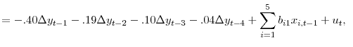
The first DGP, based on the empirical relationship between the change in core inflation (
![]() ) and the output gap (
) and the output gap (![]() ), takes the form
), takes the form
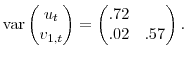
We consider experiments with two different settings of
The second DGP, based on estimated relationships among inflation (
![]() ), the output gap (
), the output gap (![]() ), and food and energy price inflation
(
), and food and energy price inflation
(![]() ), takes the form:
), takes the form:
As with DGP 1, we consider experiments with two settings of the set of
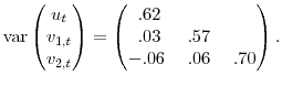
The third DGP, based on estimated relationships among inflation (
![]() ) and five business cycle factors estimated as in Stock and Watson (2005) (
) and five business cycle factors estimated as in Stock and Watson (2005) (
![]() ), takes the form:
), takes the form:
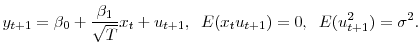
 var
var |
||
 |
(12) |
As with DGPs 1 and 2, we consider experiments with two different settings of the set of
3.2 Forecast approaches
Following practices common in the literature from which our applications are taken (see, e.g., Stock and Watson (2003)), direct multi-step forecasts one and four steps ahead are formed from various combinations of estimates of the following forecasting models:
where
We examine the accuracy of forecasts from: (1) OLS estimates of the restricted model (13); (2) OLS estimates of the unrestricted model (14); (3) the "known" optimal linear combination of the restricted and unrestricted forecasts, using the weight
implied by equation (4) and population moments implied by the DGP; (4) the estimated optimal linear combination of the restricted and unrestricted forecasts, using the weight given in (8) and estimated moments of the data; (5) the estimated optimal
linear combination using the Stein rule-variant weight given in (9); and (6) a simple average of the restricted and unrestricted forecasts (as noted above, weights of 1/2 are optimal if the signal associated with the ![]() variables equals the noise, making the models equally accurate).
variables equals the noise, making the models equally accurate).
3.3 Simulation results
In our Monte Carlo comparison of methods, we primarily base our evaluation on average MSEs over a range of forecast samples. For simplicity, in presenting average MSEs, we only report actual average MSEs for the restricted model (13). For all other forecasts, we report the ratio of a forecast's average MSE to the restricted model's average MSE. To capture potential differences in MSE distributions, we also present some evidence on the probabilities of equaling or beating the restricted model.
3.3.1 Results for signal = noise experiments
We begin with the case in which the coefficients ![]() (elements of
(elements of
![]() ) on the lags of
) on the lags of ![]() (elements of
(elements of ![]() ) in the DGPs (10)-(12) are set such that, at the 1-step ahead horizon, the restricted and unrestricted model forecasts for period
) in the DGPs (10)-(12) are set such that, at the 1-step ahead horizon, the restricted and unrestricted model forecasts for period ![]() are expected to be equally accurate -- because the signal and noise associated with the
are expected to be equally accurate -- because the signal and noise associated with the ![]() variables are equalized as
of that period. In this setting, the optimally combined forecast should, on average, be more accurate than either the restricted or unrestricted forecasts. Note, however, that the models are scaled to make only 1-step ahead forecasts equally accurate. At the 4-step ahead forecast horizon, the
restricted model may be more or less accurate than the unrestricted, depending on the DGP.
variables are equalized as
of that period. In this setting, the optimally combined forecast should, on average, be more accurate than either the restricted or unrestricted forecasts. Note, however, that the models are scaled to make only 1-step ahead forecasts equally accurate. At the 4-step ahead forecast horizon, the
restricted model may be more or less accurate than the unrestricted, depending on the DGP.
The average MSE results reported in Table 1 confirm the theoretical implications. Consider first the 1-step ahead horizon. With all three DGPs, the ratio of the unrestricted model's average MSE to the restricted model's average MSE is close to 1.000 for all forecast samples. At the 4-step ahead
horizon, for all DGPs the ratio of the unrestricted model's average MSE to the restricted model's average MSE is generally above 1.000. The unrestricted model fares especially poorly relative to the restricted in the case of DGP 3, in which the unrestricted model includes five more variables than
the restricted. In general, in all cases, the MSE ratios for 4-step ahead forecasts from the unrestricted model tend to fall as ![]() rises, reflecting the increase in the precision of the
rises, reflecting the increase in the precision of the
![]() coefficient (
coefficient (
![]() ) estimates that occurs as forecasting moves forward in time and the model estimation sample grows.
) estimates that occurs as forecasting moves forward in time and the model estimation sample grows.
A combination of the restricted and unrestricted forecasts has a lower average MSE, with the gains generally increasing in the number of variables omitted from the restricted model and the forecast horizon. At the 1-step horizon, using the known optimal combination weight
![]() yields
yields ![]() = 20 MSE ratios of .994, .983, and .974 for, respectively,
DGPs 1, 2, and 3. At the 4-step horizon, the forecast based on the known optimal combination weight has
= 20 MSE ratios of .994, .983, and .974 for, respectively,
DGPs 1, 2, and 3. At the 4-step horizon, the forecast based on the known optimal combination weight has ![]() = 20 MSE ratios of .986, .962, and .973 for DGPs 1-3.9
= 20 MSE ratios of .986, .962, and .973 for DGPs 1-3.9
Not surprisingly, having to estimate the optimal combination weight tends to slightly reduce the gains to combination. For example, in the case of DGP 2 and ![]() , the MSE ratio for the
estimated optimal combination forecast is .989, compared to .983 for the known optimal combination forecast. Using the Stein rule-based adjustment to the optimal combination estimate (based on equation (9)) has mixed consequences, sometimes faring a bit worse than the
directly estimated optimal combination forecast (based on equation (8)) and sometimes a bit worse. To use the same DGP 2 example, the
, the MSE ratio for the
estimated optimal combination forecast is .989, compared to .983 for the known optimal combination forecast. Using the Stein rule-based adjustment to the optimal combination estimate (based on equation (9)) has mixed consequences, sometimes faring a bit worse than the
directly estimated optimal combination forecast (based on equation (8)) and sometimes a bit worse. To use the same DGP 2 example, the ![]() = 20 MSE ratio for the Stein version
of the estimated optimal combination is .990, compared to .989 for the directly estimated optimal combination. However, in the case of 4-step ahead forecasts for DGP 3 with the
= 20 MSE ratio for the Stein version
of the estimated optimal combination is .990, compared to .989 for the directly estimated optimal combination. However, in the case of 4-step ahead forecasts for DGP 3 with the ![]() sample,
the MSE ratios of the known
sample,
the MSE ratios of the known
![]() , estimated
, estimated
![]() , and Stein-adjusted
, and Stein-adjusted
![]() are, respectively, .973, .991, and .985.
are, respectively, .973, .991, and .985.
In the Table 1 experiments, the simple average of the restricted and unrestricted forecasts is consistently a bit more accurate than the estimated optimal combination forecast. For example, for DGP 3 and the ![]() = 20 forecast sample, the MSE ratio of the simple average forecast is .974 for both 1-step and 4-step ahead forecasts, compared to the estimated optimal combination forecasts' MSE ratios of .982 (1-step) and .991 (4-step). There are two reasons a simple average fares so well.
First, with the DGPs parameterized to make signal = noise for one-step ahead forecasts for period
= 20 forecast sample, the MSE ratio of the simple average forecast is .974 for both 1-step and 4-step ahead forecasts, compared to the estimated optimal combination forecasts' MSE ratios of .982 (1-step) and .991 (4-step). There are two reasons a simple average fares so well.
First, with the DGPs parameterized to make signal = noise for one-step ahead forecasts for period ![]() , the theoretically optimal combination weight is 1/2. Of course, as forecasting moves
forward in time, the theoretically optimal combination weight declines, because as more and more data become available for estimation, the signal-to-noise ratio rises (e.g., in the case of DGP 3, the known optimal weight for the forecast of the 80th observation in the prediction sample is about
.33). But the decline is gradual enough that only late in a long forecast sample would noticeable differences emerge between the theoretically optimal combination forecast and the simple average. A second reason is that, in practice, the optimal combination weight may not be estimated with much
precision. As a result, imposing a fixed weight of 1/2 is likely better than trying to estimate a weight that is not dramatically different from 1/2.
, the theoretically optimal combination weight is 1/2. Of course, as forecasting moves
forward in time, the theoretically optimal combination weight declines, because as more and more data become available for estimation, the signal-to-noise ratio rises (e.g., in the case of DGP 3, the known optimal weight for the forecast of the 80th observation in the prediction sample is about
.33). But the decline is gradual enough that only late in a long forecast sample would noticeable differences emerge between the theoretically optimal combination forecast and the simple average. A second reason is that, in practice, the optimal combination weight may not be estimated with much
precision. As a result, imposing a fixed weight of 1/2 is likely better than trying to estimate a weight that is not dramatically different from 1/2.
3.3.2 Results for signal noise experiments
In DGPs with larger ![]() (
(
![]() ) coefficients -- specifically, coefficient values set to those obtained from empirical estimates of inflation models -- the signal associated with the
) coefficients -- specifically, coefficient values set to those obtained from empirical estimates of inflation models -- the signal associated with the ![]() (
(![]() ) variables exceeds the noise, such that the unrestricted model is expected to
be more accurate than the restricted model. In this setting, too, our asymptotic results imply the optimal combination forecast should be more accurate than the unrestricted model forecast, on average. However, relative to the accuracy of the unrestricted model forecast, the gains to combination
should be smaller than in DGPs with smaller
) variables exceeds the noise, such that the unrestricted model is expected to
be more accurate than the restricted model. In this setting, too, our asymptotic results imply the optimal combination forecast should be more accurate than the unrestricted model forecast, on average. However, relative to the accuracy of the unrestricted model forecast, the gains to combination
should be smaller than in DGPs with smaller ![]() coefficients.
coefficients.
The results for DGPs 1-3 reported in Table 2 confirm these theoretical implications. At the 1-step ahead horizon, the unrestricted model's average MSE is about 5-6 percent lower than the restricted model's MSE in DGP 1 and 3 experiments and roughly 15 percent lower in DGP 2 experiments. At the 4-step ahead horizon, the unrestricted model is more accurate than the restricted by about 12, 28, and 4 percent for DGPs 1, 2, and 3.
Combination using the known optimal combination weight
![]() improves accuracy further, more so for DGP 3 (for which the unrestricted forecasting model is largest) than DGPs 1 and 2 and more so for the 4-step ahead horizon than the
1-step horizon. Consider, for example, the forecast sample
improves accuracy further, more so for DGP 3 (for which the unrestricted forecasting model is largest) than DGPs 1 and 2 and more so for the 4-step ahead horizon than the
1-step horizon. Consider, for example, the forecast sample ![]() = 1. For DGP 2, the known optimal combination forecast's MSE ratios are .839 (1-step) and .716 (4-step), compared to the
unrestricted forecast's MSE ratios of, respectively, .845 and .723. For DGP 3, the known optimal combination forecast's MSE ratios are .924 (1-step) and .919 (4-step), compared to the unrestricted forecast's MSE ratios of, respectively, .947 and .971. Consistent with our theoretical results, the
gains to combination seem to be larger under conditions that likely reduce parameter estimation precision (more variables and residual serial correlation created by the multi-step forecast horizon).
= 1. For DGP 2, the known optimal combination forecast's MSE ratios are .839 (1-step) and .716 (4-step), compared to the
unrestricted forecast's MSE ratios of, respectively, .845 and .723. For DGP 3, the known optimal combination forecast's MSE ratios are .924 (1-step) and .919 (4-step), compared to the unrestricted forecast's MSE ratios of, respectively, .947 and .971. Consistent with our theoretical results, the
gains to combination seem to be larger under conditions that likely reduce parameter estimation precision (more variables and residual serial correlation created by the multi-step forecast horizon).
Similarly, the gains to combination (gains relative to the unrestricted model's forecast) rise as the estimation sample gets smaller. Table 3 reports results for the same DGPs used in Table 2, but for the case in which the initial estimation sample is 40 observations instead of 80. With the smaller estimation sample, DGP 2 simulations yield known optimal combination MSE ratios of .882 (1-step) and .807 (4-step), compared to the unrestricted forecast's MSE ratios of, respectively, .908 and .851. For DGP 3, the known optimal combination forecast's MSE ratios are .960 (1-step) and .959 (4-step), compared to the unrestricted forecast's MSE ratios of, respectively, 1.064 and 1.146.
Again, not surprisingly, having to estimate the optimal combination weight tends to slightly reduce the gains to combination. For instance, in Table 2's results for case DGP 2 and ![]() = 1,
the 4-step ahead MSE ratio for the estimated optimal combination forecast is .723, compared to .716 for the known optimal combination forecast. Using the Stein rule-based adjustment to the optimal combination estimate (based on equation (9)) typically reduces forecast
accuracy a bit more (to a MSE ratio of .732 in the same example), but not always -- the adjustment often improves forecast accuracy with DGP 3 and a small estimation sample (Table 3).
= 1,
the 4-step ahead MSE ratio for the estimated optimal combination forecast is .723, compared to .716 for the known optimal combination forecast. Using the Stein rule-based adjustment to the optimal combination estimate (based on equation (9)) typically reduces forecast
accuracy a bit more (to a MSE ratio of .732 in the same example), but not always -- the adjustment often improves forecast accuracy with DGP 3 and a small estimation sample (Table 3).
Imposing simple equal weights in averaging the unrestricted and restricted model forecasts sometimes slightly improves upon the estimated optimal combination but other times reduces accuracy. In Table 2's results for DGPs 1 and 2, the estimated optimal combination is always more accurate than
the simple average. For example, with DGP 2 and the 4-step horizon, the ![]() = 20 MSE ratio of the estimated optimal combination forecast is .725, compared to the simple average forecast's MSE
ratio of .767. But for DGP 3, the simple average is often slightly more accurate than the estimated optimal combination. For instance, at the 4-step horizon and with
= 20 MSE ratio of the estimated optimal combination forecast is .725, compared to the simple average forecast's MSE
ratio of .767. But for DGP 3, the simple average is often slightly more accurate than the estimated optimal combination. For instance, at the 4-step horizon and with ![]() = 20, the optimal
combination and simple average forecast MSEs are, respectively, .928 and .919.
= 20, the optimal
combination and simple average forecast MSEs are, respectively, .928 and .919.
As these results suggest, the merits of imposing equal combination weights over estimating weights depend on how far the true optimal weight is from 1/2 (which depends on the population size and precision of the model coefficients) and the precision of the estimated combination weight. In cases
in which the known optimal weight is relatively close to 1/2 (DGP 3, 1-step forecast, Table 2), the simple average performs quite similarly to the known optimal forecast, and better than the estimated optimal combination. In cases in which the known optimal weight is far from 1/2 (DGP 2, 1-step
forecast, Table 2), the simple average is dominated by the known optimal forecast and, in turn, the estimated optimal combination. Consistent with such reasoning, reducing the initial estimation sample generally improves the accuracy of the simple average forecast relative to the estimated optimal
combination. For example, Table 3 shows that, with DGP 2 and the 4-step horizon, the ![]() = 20 MSE ratio of the simple average forecast is .789, compared to the estimated optimal combination
forecast's MSE ratio of .775 (in Table 2, the corresponding figures are .767 and .725).
= 20 MSE ratio of the simple average forecast is .789, compared to the estimated optimal combination
forecast's MSE ratio of .775 (in Table 2, the corresponding figures are .767 and .725).
3.3.3 Distributional results
In addition to helping to lower the average forecast MSE, combination of restricted and unrestricted forecasts helps to tighten the distribution of relative accuracy -- specifically, the MSE relative to the MSE of the restricted model. The results in Table 4 indicate that combination --
especially simple averaging -- often increases the probability of equaling or beating the MSE of the restricted model, often by more than it lowers average MSE (note that, to conserve space, the table omits results for DGP 1). For instance, with DGP 2 parameterized such that signal = noise for
forecasting 1-step ahead to period ![]() , the frequency with which the unrestricted model's MSE is less than or equal to the restricted model's MSE is 47.2 percent for
, the frequency with which the unrestricted model's MSE is less than or equal to the restricted model's MSE is 47.2 percent for ![]() = 20. The frequency with which the known optimal combination forecast's MSE is below the restricted model's MSE is 57.4 percent. Although the estimated combination does not fare as well (probability of
51.4 percent), a simple average fares even better, beating the MSE of the restricted model in 58.1 percent of the simulations. Note also that, by this distributional metric, using the Stein variant of the combination weight estimate often offers a material advantage over the direct approach to
estimating the combination weight. In the same example, the Stein-based combination forecast has a probability of 55.3 percent, compared to the 51.4 percent for the directly estimated combination forecast.
= 20. The frequency with which the known optimal combination forecast's MSE is below the restricted model's MSE is 57.4 percent. Although the estimated combination does not fare as well (probability of
51.4 percent), a simple average fares even better, beating the MSE of the restricted model in 58.1 percent of the simulations. Note also that, by this distributional metric, using the Stein variant of the combination weight estimate often offers a material advantage over the direct approach to
estimating the combination weight. In the same example, the Stein-based combination forecast has a probability of 55.3 percent, compared to the 51.4 percent for the directly estimated combination forecast.
By this probability metric, the simple average (and, to a lesser extent, the optimal combination based on the Stein rule estimate) also fares well in other experiments. Consider, for example, the experiments with the signal noise version of DGP 3, a forecast horizon of 4 steps, and ![]() = 20. In this case, the probability the unrestricted model yields a MSE less than or equal
to the restricted model's MSE is 54.3 percent. The probabilities for the estimated optimal combination, Stein-estimated optimal combination, and simple average are, respectively, 62.9, 64.9, and 69.1 percent. Again, averaging, especially simple averaging, greatly improves the probability of beating
the accuracy of the restricted model forecast.
= 20. In this case, the probability the unrestricted model yields a MSE less than or equal
to the restricted model's MSE is 54.3 percent. The probabilities for the estimated optimal combination, Stein-estimated optimal combination, and simple average are, respectively, 62.9, 64.9, and 69.1 percent. Again, averaging, especially simple averaging, greatly improves the probability of beating
the accuracy of the restricted model forecast.
4 Empirical Applications
To evaluate the empirical performance of our proposed forecast methods compared to some related alternatives (described below), we consider the widely studied problem of forecasting inflation with Phillips curve models. In particular, we examine forecasts of quarterly core PCE (U.S.) inflation. In light of the potential for the benefits of forecast combination to rise as the number of variables and, in turn, overall parameter estimation imprecision increases, we consider a range of applications, including between one and five predictors of core inflation. In a first application, patterned on analyses in such studies as Stock and Watson (1999, 2003), Orphanides and van Norden (2005), and Clark and McCracken (2006), the unrestricted forecasting model includes lags of inflation and the output gap. In a second application, the unrestricted forecasting model is augmented to include lags of food and energy price inflation, following Gordon's (1998) approach of including supply shock measures in the Phillips curve. In another set of applications, patterned on such studies as Brave and Fisher (2004), Stock and Watson (2002, 2005), and Boivin and Ng (2005), the unrestricted forecast model includes lags of inflation and 1, 2, 3, or 5 common business cycle factors, estimated as in Stock and Watson (2005). This section proceeds by detailing the data and forecasting models, describing some additional forecast methods included for comparison, and presenting the results.
4.1 Data and model details
Inflation is measured in annualized percentage terms (as 400 times the log change in the price index).10 The output gap is measured as the log of real
GDP less the log of CBO's estimate of potential GDP. Following Gordon (1998), the food and energy price inflation variable is measured as overall PCE inflation less core PCE inflation. The common factors are estimated with the principal component approach of Stock and Watson (2002, 2005), using a
data set of 127 monthly series nearly identical to Stock and Watson's (2005).11 Following the specifications of Stock and Watson (2005), we first
transformed the data for stationarity, screened for outliers, and standardized the data, and then computed principal components at the monthly frequency. Following Stock and Watson (2005) and Boivin and Ng (2005), the factors are estimated recursively for each month of the forecast sample, applying
the factor estimation algorithm to data through the given month. Quarterly data on factors used in model estimation ending in quarter ![]() are within-quarter averages of monthly factors
estimated with data from the beginning of the sample through the last month of quarter
are within-quarter averages of monthly factors
estimated with data from the beginning of the sample through the last month of quarter ![]()
Following the basic approach of Stock and Watson (1999, 2003), among others, we treat inflation as having a unit root, and forecast a measure of the direct multi-step change in inflation as a function of lags of the change in quarterly inflation and lags of other variables. In particular, using
the notation of the last section, we make ![]() the log difference of the quarterly core PCE price index (scaled by 400 to make
the log difference of the quarterly core PCE price index (scaled by 400 to make ![]() an annualized percentage change);
an annualized percentage change); ![]() is then the change in quarterly inflation. The predictand is
is then the change in quarterly inflation. The predictand is
![]() , where
, where
![]() denotes the average annual rate of price change from
denotes the average annual rate of price change from ![]() to
to
![]() . The
. The ![]() variables denote the output gap, relative food and energy price
inflation, and the set of common factors included in the model (with the number ranging from 1 to 5). The restricted model is autoregressive -- the multi-step change in inflation is a function of just lags of the one-period change in inflation. The unrestricted model adds lags of
variables denote the output gap, relative food and energy price
inflation, and the set of common factors included in the model (with the number ranging from 1 to 5). The restricted model is autoregressive -- the multi-step change in inflation is a function of just lags of the one-period change in inflation. The unrestricted model adds lags of ![]() variables to the set of regressors. In particular, the competing forecasting models take the forms of section 4's equations (13) and (14). All models include
four lags of the change in inflation (
variables to the set of regressors. In particular, the competing forecasting models take the forms of section 4's equations (13) and (14). All models include
four lags of the change in inflation (
![]() ). For the output gap and the factors, the models use one lag. For food-energy inflation, the models include two lags.
). For the output gap and the factors, the models use one lag. For food-energy inflation, the models include two lags.
The forecasting models are estimated with data starting in 1961:Q1. The parameters of the forecasting models are re-estimated with added data as forecasting moves forward through time (that is, our forecasting scheme is the so-called recursive). The forecast sample is 1985:Q1 (1985:Q4 for four-step ahead forecasts) through 2006:Q2. We report results -- MSEs -- for forecast horizons of one quarter and one year.
4.2 Additional forecast methods
Because our proposed forecast combination methods correspond to a form of shrinkage, for comparison we supplement our results to include not only our proposed methods but also some alternative shrinkage forecasts based on Bayesian methods. Doan, Litterman, and Sims (1984) suggest that conventional Bayesian estimation (specifically, the prior) provides a flexible method for balancing the tradeoff between signal and parameter estimation noise.
Accordingly, one alternative forecast is obtained from the unrestricted forecasting model (for a given application) estimated with generalized ridge regression, which is similar to and under some implementations identical to conventional BVAR estimation. Consistent with the spirit of our
proposed combination approaches, which try to limit the effects of sampling noise in the coefficients of the ![]() variables, the ridge estimator pushes the coefficients on the
variables, the ridge estimator pushes the coefficients on the ![]() variables toward zero by imposing informative prior variances on the associated coefficients (note that the tightness of the prior increases with the number of lags of
variables toward zero by imposing informative prior variances on the associated coefficients (note that the tightness of the prior increases with the number of lags of ![]() included). The ridge estimator allows very large variances on the coefficients of the intercept and lagged inflation terms. In the case of the 1-step ahead model, our generalized ridge estimator is exactly the same as the
conventional Bayesian or BVAR estimator of Litterman (1986), except that we use flat priors on the intercept and lagged inflation terms.12 We apply the
same priors to the 4-step ahead model (based on some experimentation to ensure the prior setting worked well).
included). The ridge estimator allows very large variances on the coefficients of the intercept and lagged inflation terms. In the case of the 1-step ahead model, our generalized ridge estimator is exactly the same as the
conventional Bayesian or BVAR estimator of Litterman (1986), except that we use flat priors on the intercept and lagged inflation terms.12 We apply the
same priors to the 4-step ahead model (based on some experimentation to ensure the prior setting worked well).
We report a second alternative forecast constructed by applying Bayesian model averaging (BMA) to the restricted and unrestricted models, following the BMA approach of Fernandez, Ley, and Steel (2001). In particular, we first estimate the models imposing a simple ![]() -prior (but with a flat prior on intercepts), and then average the models based on posterior probabilities calculated as in Fernandez, Ley, and Steel (2001). Based on Wright's (2003) findings on forecasting inflation
with BMA methods, we set the
-prior (but with a flat prior on intercepts), and then average the models based on posterior probabilities calculated as in Fernandez, Ley, and Steel (2001). Based on Wright's (2003) findings on forecasting inflation
with BMA methods, we set the ![]() -prior coefficient (
-prior coefficient (![]() in the notation of
Fernandez, et al., or
in the notation of
Fernandez, et al., or ![]() in Wright's notation) at .20.
in Wright's notation) at .20.
4.3 Results
In very broad terms, the results in Table 5 seem reasonably reflective of the overall literature on forecasting U.S. inflation in data since the mid-1980s: the variables included in the unrestricted model but not the restricted only sometimes improve forecast accuracy. Across the 12 columns of Table 5 (covering six applications and two forecast horizons), the restricted model's MSE is lower than the unrestricted model's in six cases, sometimes slightly (e.g., 1-year ahead forecasts from the model with five factors) and sometimes dramatically (e.g., 1-year ahead forecasts from the model with the output gap and food-energy inflation).
Combining forecasts with our proposed methods significantly improves upon the accuracy of the unrestricted model's forecast, by enough that, in each column, at least one of the average forecasts is more accurate than the restricted model's forecast. For every application and horizon, our
estimated optimal combination forecast has a lower MSE than the unrestricted model. For example, in the three factor application (lower block, middle), the optimal combination forecast has a 1-year ahead MSE ratio of .791, while the unrestricted model has a MSE ratio of .879. Consistent with our
theoretical results, the advantage of the combination forecast over the unrestricted forecast tends to rise as the number of ![]() variables in the unrestricted model increases (with the increase
in the number of variables tending to lower the signal-noise ratio) and as the forecast horizon increases. For example, in the same (three factor) application, the 1-quarter ahead MSE ratios of the unrestricted and optimal combination forecasts are, respectively, .950 and .935 -- closer together
than for the 1-year ahead horizon. In the five factor application, the 1-year ahead MSE ratios of the unrestricted and optimal combination forecasts are 1.001 and .834 -- farther apart than in the three factor application.
variables in the unrestricted model increases (with the increase
in the number of variables tending to lower the signal-noise ratio) and as the forecast horizon increases. For example, in the same (three factor) application, the 1-quarter ahead MSE ratios of the unrestricted and optimal combination forecasts are, respectively, .950 and .935 -- closer together
than for the 1-year ahead horizon. In the five factor application, the 1-year ahead MSE ratios of the unrestricted and optimal combination forecasts are 1.001 and .834 -- farther apart than in the three factor application.
Estimating the optimal combination weight with our proposed Stein rule-based approach yields a consistent, modest improvement in forecast accuracy. In all columns of Table 5, the optimal combination forecast based on the Stein-estimated weight (9) has a lower MSE than does the optimal combination based on the baseline approach (8). In the same three factor application, at the 1-year horizon the optimal combination based on the Stein-estimated weight has a MSE ratio of .781, compared to the directly estimated optimal combination forecast's MSE ratio of .791. With five factors and the 1-year horizon, the Stein-estimated optimal combination's MSE ratio is .807, while the directly estimated optimal combination forecast's MSE ratio is .834.
In most cases, imposing equal weights in combining the restricted and unrestricted model forecasts further improves forecast accuracy, sometimes substantially. As a result, in many cases, the simple average forecast is the best forecast of all considered. For instance, in the output gap and food-energy inflation application, the 1-year ahead MSE ratios of the simple average and Stein-estimated combination forecasts are .871 (the lowest among all forecasts) and 1.020, respectively. In the application with two factors, the 1-year ahead MSE ratios are .854 (again, the lowest among all forecasts) and .866 for, respectively, the simple average and Stein-estimated combination forecasts. In some cases, though, the simple average is only slightly better than or worse than our proposed Stein rule-based approach. For example, in the three factor application, the simple average forecast's 1-year ahead MSE ratio is .782, compared to the Stein-estimated combination forecast's MSE ratio of .781.
In these applications, our proposed combinations clearly dominate Bayesian model averaging and are generally about as good as or better than ridge regression.13 For example, in the two factor application, the 1-year ahead MSE ratio is .866 for the Stein-estimated combination, .854 for the simple average, and .891 for the ridge regression forecast. In the same application, though, the 1-quarter ahead MSE ratios are virtually identical, at .953, .950, and .950, respectively. In the application with the output gap and food-energy inflation as predictands, the 1-quarter ahead MSE ratios of the Stein-estimated, simple average, and ridge regression forecasts are, respectively, 1.060, .983, and 1.032. However, in all cases, the BMA forecast is less accurate than the Stein-estimated combination and simple average forecasts. For instance, in the two factor application, the BMA forecast has MSE ratios of .971 and .934 at the 1-quarter and 1-year ahead horizons (compared, e.g., to the Stein-estimated combination MSE ratios of .953 and .866).
5 Conclusion
As reflected in the principle of parsimony, when some variables are truly but weakly related to the variable being forecast, having the additional variables in the model may detract from forecast accuracy, because of parameter estimation error. Focusing on such cases of weak predictability, we show that combining the forecasts of the parsimonious and larger models can improve forecast accuracy. We first derive, theoretically, the optimal combination weight and combination benefit. In the special case in which the coefficients on the variables of interest are of a magnitude that makes the restricted and unrestricted models equally accurate, the MSE-minimizing forecast is a simple, equally-weighted average of the restricted and unrestricted forecasts. A range of Monte Carlo experiments and empirical examples show our proposed approach of combining forecasts from nested models to be effective in practice.
6 Appendix 1: Theory Details
Note that, in the notation below, ![]() denotes a standard (
denotes a standard (![]() Brownian motion.
Brownian motion.
Proof of Theorem 1: The proof is provided in two stages. In the first stage we provide an asymptotic expansion. In the second we apply a functional central limit theorem and a weak convergence to stochastic integrals result, both from De Jong and Davidson (2000).
In the first stage we show that
To do so first note that straightforward algebra reveals that
We must then show that each bracketed term from (15) corresponds to that in (16). For brevity we will show this in detail only for the first bracketed term. The second and third follow from similar arguments.
Consider the first bracketed term in (16). If we add and subtract
![]() in the first component, and rearrange terms we obtain
in the first component, and rearrange terms we obtain
The first right-hand side term is the desired result. For the second right-hand side term first note that Assumptions 3 and 4 suffice for each of ![]() ,
,
![]() and
and
![]() to converge weakly. Applying Theorem 3.2 of de Jong and Davidson (2000) then implies that the second right-hand
side term is
to converge weakly. Applying Theorem 3.2 of de Jong and Davidson (2000) then implies that the second right-hand
side term is ![]() and the proof is complete.
and the proof is complete.
For the second, third and fourth components of the first bracketed term note that adding and subtracting ![]() ,
,
![]() ,
, ![]() and
and
![]() provides
provides
Note that the weighted sum of the first right-hand side term of each of (17) - (19) gives us
the second right-hand side term in (15). We must therefore show that all of the remaining right-hand side terms in (17)-(19) are ![]() The proof of each is very similar. For example, taking the absolute value of the fifth right-hand side term in (17) provides
The proof of each is very similar. For example, taking the absolute value of the fifth right-hand side term in (17) provides
Since assumptions 3 and 4 suffice for
For the second stage of the proof we show that the expansion in (15) converges in distribution to the term provided in the Theorem. To do so recall that Assumption 4 implies
![]() . Also, Assumptions 3 (a) - (d) imply
. Also, Assumptions 3 (a) - (d) imply
![]() . Continuity then provides the desired results for the second contribution to the first bracketed term, for the second and third contributions
to the second bracketed term and the third bracketed term.
. Continuity then provides the desired results for the second contribution to the first bracketed term, for the second and third contributions
to the second bracketed term and the third bracketed term.
The remaining two contributions (the first in each of the first two bracketed terms), are each weighted sums of increments
![]() . Consider the first contribution to the second bracketed term. Since this increment satisfies Assumption 3 (d) and has an associated long-run variance
. Consider the first contribution to the second bracketed term. Since this increment satisfies Assumption 3 (d) and has an associated long-run variance ![]() , we can apply Theorem 4.1 of De Jong and Davidson (2000) directly to obtain the desired convergence in distribution
, we can apply Theorem 4.1 of De Jong and Davidson (2000) directly to obtain the desired convergence in distribution

 |
Note the addition of the drift term
Proof of Corollary 1: First note that the assumptions, and notably Assumption 3 (c), suffice for uniform integrability of the difference in MSEs and hence the limit of the expectation converges to the expectation of the limit. Second, note that both the second bracketed term and the first component of the first bracketed term are zero mean and moreover, the third bracketed term is nonstochastic. Taking expectations of the limit we then obtain
 |
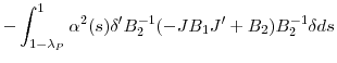
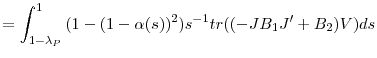
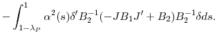
||
![\displaystyle ={\{}0+\int_{1-\lambda_{P}}^{1}{(1-(1-\alpha(s))^{2})s^{-2}E[{W}^{\prime }(s)V^{1/2}(-JB_{1}{J}^{\prime}+B_{2})V^{1/2}W(s)]ds\}}](img267.gif) |
||
 |
||
V)ds}](img269.gif) |
||
 |
||
 |
||
 |
Proof of Corollary 2: We obtain our pointwise optimal combining weight by maximizing, for each fixed ![]() , the argument of the integral in Corollary 1. That is we
choose
, the argument of the integral in Corollary 1. That is we
choose ![]() to maximize
to maximize
Differentiating (20) with respect to
Setting the FOC to zero and solving for ![]() provides the formula from the Corollary. The SOC is negative at this solution and we obtain the desired result.
provides the formula from the Corollary. The SOC is negative at this solution and we obtain the desired result.
Atkeson, A., and Ohanian, L.E. (2001), "Are Phillips Curves Useful for Forecasting Inflation?" Quarterly Review, Federal Reserve Bank of Minneapolis, 25, 2-11.
Bates, J.M., and Granger, C.W.J. (1969), "The Combination of Forecasts," Operations Research Quarterly, 20, 451-468.
Boivin, J., and Ng, S. (2005), "Understanding and Comparing Factor-Based Forecasts," International Journal of Central Banking, 1, 117-151.
Brave, S., and Fisher, J.D.M. (2004), "In Search of a Robust Inflation Forecast," Economic Perspectives, Federal Reserve Bank of Chicago, Fourth Quarter, 12-31.
Clark, T.E., and McCracken, M.W. (2005), "Evaluating Direct Multistep Forecasts," Econometric Reviews, 24, 369-404.
Clark, T.E., and McCracken, M.W. (2006), "The Predictive Content of the Output Gap for Inflation: Resolving In-Sample and Out-of-Sample Evidence," Journal of Money, Credit, and Banking, 38, 1127-1148.
Clark, T.E., and West, K.D. (2006a), "Using Out-of-Sample Mean Squared Prediction Errors to Test the Martingale Difference Hypothesis," Journal of Econometrics, 135, 155-186.
Clark, T.E., and West, K.D. (2006b), "Approximately Normal Tests for Equal Predictive Accuracy in Nested Models," Journal of Econometrics, forthcoming.
Clements, M.P., and Hendry, D.F. (1998), Forecasting Economic Time Series, Cambridge, U.K.: Cambridge University Press.
de Jong, R.M., and Davidson, J. (2000), "The Functional Central Limit Theorem and Weak Convergence to Stochastic Integrals I: Weakly Dependent Processes," Econometric Theory, 16, 621-642.
Diebold, F.X. (1998), Elements of Forecasting, Cincinnati, OH: South-Western College Publishing.
Doan, T., Litterman, R., and Sims, C. (1984), "Forecasting and Conditional Prediction Using Realistic Prior Distributions," Econometric Reviews, 3, 1-100.
Elliott, G., and Timmermann, A. (2004), "Optimal Forecast Combinations Under General Loss Functions and Forecast Error Distributions," Journal of Econometrics, 122, 47-79.
Fernandez, C., Ley, E., and Steel, M.F.J. (2001), "Benchmark Priors for Bayesian Model Averaging," Journal of Econometrics, 100, 381-427.
Godfrey, L.G., and Orme, C.D. (2004), "Controlling the Finite Sample Significance Levels of Heteroskedasticity-Robust Tests of Several Linear Restrictions on Regression Coefficients," Economics Letters, 82, 281-287.
Gordon, R.J. (1998), "Foundations of the Goldilocks Economy: Supply Shocks and the Time-Varying NAIRU," Brookings Papers on Economic Activity (no. 2), 297-346.
Goyal, A., and Welch, I. (2003), "Predicting the Equity Premium with Dividend Ratios," Management Science, 49, 639-654.
Hansen, B.E. (1992), "Convergence to Stochastic Integrals for Dependent Heterogeneous Processes, Econometric Theory, 8, 489-500.
Hendry, D.F., and Clements, M.P. (2004), "Pooling of Forecasts," Econometrics Journal, 7, 1-31.
Jacobson, T., and Karlsson, S. (2004), "Finding Good Predictors for Inflation: A Bayesian Model Averaging Approach," Journal of Forecasting, 23, 479-496.
Koop, G., and Potter, S. (2004), "Forecasting in Dynamic Factor Models Using Bayesian Model Averaging," Econometrics Journal, 7, 550-565.
Litterman, R.B. (1986), "Forecasting with Bayesian Vector Autoregressions -- Five Years of Experience," Journal of Business and Economic Statistics, 4, 25-38.
Newey, W.K., and West, K.D. (1987), "A Simple, Positive Semi-Definite, Heteroskedasticity and Autocorrelation Consistent Covariance Matrix," Econometrica, 55, 703-708.
Orphanides, A., and van Norden, S. (2005), "The Reliability of Inflation Forecasts Based on Output Gap Estimates in Real Time," Journal of Money, Credit, and Banking, 37, 583-601.
Stock, J.H., and Watson, M.W. (1999), "Forecasting Inflation," Journal of Monetary Economics, 44, 293-335.
Stock, J.H., and Watson, M.W. (2002), "Macroeconomic Forecasting Using Diffusion Indexes," Journal of Business and Economic Statistics, 20, 147-162.
Stock, J.H., and Watson, M.W. (2003), "Forecasting Output and Inflation: The Role of Asset Prices," Journal of Economic Literature, 41, 788-829.
Stock, J.H., and Watson, M.W. (2005), "An Empirical Comparison of Methods for Forecasting Using Many Predictors," manuscript, Harvard University.
Theil, H. (1971), Principles of Econometrics, New York: John Wiley Press.
Timmermann, A. (2006), "Forecast Combinations," in Handbook of Forecasting, eds. G. Elliott, C.W.J. Granger, and A. Timmermann, North Holland, 135-196.
Wright, J.H. (2003), "Forecasting U.S. Inflation by Bayesian Model Averaging," manuscript, Board of Governors of the Federal Reserve System.
| method/model | horizon=1, |
horizon=1, |
horizon=1, |
horizon=1, |
horizon=4, |
horizon=4, |
horizon=4, |
horizon=4, |
|---|---|---|---|---|---|---|---|---|
| DGP 1: restricted | .773 | .775 | .771 | .764 | .818 | .816 | .808 | .796 |
| DGP 1: unrestricted | 1.004 | 1.002 | 1.000 | .998 | 1.029 | 1.011 | 1.006 | .998 |
| DGP 1: opt. combination: known
|
.995 | .994 | .994 | .993 | .995 | .986 | .985 | .982 |
| DGP 1: opt. combination:
|
.999 | .998 | .997 | .996 | 1.007 | .996 | .993 | .989 |
| DGP 1: opt. combination: Stein
|
.999 | .998 | .998 | .997 | 1.005 | .996 | .994 | .991 |
| DGP 1: simple average | .995 | .994 | .994 | .993 | .992 | .984 | .983 | .981 |
| DGP 2: restricted | .678 | .678 | .677 | .672 | .635 | .632 | .627 | .620 |
| DGP 2: unrestricted | 1.009 | 1.003 | .999 | .993 | 1.004 | 1.004 | .996 | .983 |
| DGP 2: opt. combination: known
|
.984 | .983 | .982 | .980 | .959 | .962 | .960 | .956 |
| DGP 2: opt. combination:
|
.992 | .989 | .987 | .984 | .972 | .974 | .971 | .964 |
| DGP 2: opt. combination: Stein
|
.993 | .990 | .989 | .987 | .975 | .976 | .973 | .967 |
| DGP 2: simple average | .984 | .982 | .982 | .980 | .958 | .960 | .959 | .956 |
| DGP 3: restricted | .780 | .752 | .747 | .740 | .843 | .822 | .817 | .805 |
| DGP 3: unrestricted | 1.012 | 1.009 | 1.003 | .994 | 1.058 | 1.050 | 1.037 | 1.020 |
| DGP 3: opt. combination: known
|
.974 | .974 | .973 | .970 | .972 | .973 | .971 | .967 |
| DGP 3: opt. combination:
|
.983 | .982 | .980 | .976 | .993 | .991 | .987 | .980 |
| DGP 3: opt. combination: Stein
|
.985 | .983 | .981 | .978 | .987 | .985 | .983 | .978 |
| DGP 3: simple average | .974 | .974 | .973 | .970 | .974 | .974 | .972 | .967 |
| Notes: 1. DGPs 1-3 are defined in, respectively, equations (10), (11), and (12). In all experiments, the |
|---|
Table 2. Monte Carlo Results from Signal ![]() Noise Experiments: Average MSEs(for restricted model, average MSE; for other forecasts,ratio
of average MSE to restricted model's average MSE)
Noise Experiments: Average MSEs(for restricted model, average MSE; for other forecasts,ratio
of average MSE to restricted model's average MSE)
| method/model | horizon=1, |
horizon=1, |
horizon=1, |
horizon=1, |
horizon=4, |
horizon=4, |
horizon=4, |
horizon=4, |
|---|---|---|---|---|---|---|---|---|
| DGP 1: restricted | .813 | .813 | .809 | .802 | .958 | .955 | .946 | .932 |
| DGP 1: unrestricted | .955 | .954 | .953 | .950 | .898 | .882 | .878 | .871 |
| DGP 1: opt. combination: known
|
.952 | .952 | .951 | .949 | .889 | .875 | .872 | .867 |
| DGP 1: opt. combination:
|
.957 | .955 | .954 | .952 | .895 | .881 | .878 | .872 |
| DGP 1: opt. combination: Stein
|
.960 | .958 | .957 | .954 | .903 | .888 | .884 | .877 |
| DGP 1: simple average | .959 | .959 | .958 | .958 | .896 | .890 | .889 | .887 |
| DGP 2: restricted | .811 | .805 | .803 | .798 | .967 | .948 | .940 | .929 |
| DGP 2: unrestricted | .845 | .845 | .841 | .837 | .723 | .729 | .724 | .714 |
| DGP 2: opt. combination: known
|
.839 | .840 | .837 | .834 | .716 | .721 | .718 | .710 |
| DGP 2: opt. combination:
|
.843 | .843 | .840 | .836 | .723 | .725 | .722 | .713 |
| DGP 2: opt. combination: Stein
|
.847 | .845 | .841 | .837 | .732 | .732 | .728 | .718 |
| DGP 2: simple average | .865 | .866 | .866 | .865 | .765 | .767 | .767 | .764 |
| DGP 3: restricted | .834 | .803 | .798 | .790 | .968 | .942 | .934 | .921 |
| DGP 3: unrestricted | .947 | .944 | .939 | .931 | .971 | .966 | .956 | .940 |
| DGP 3: opt. combination: known
|
.924 | .924 | .922 | .918 | .919 | .920 | .917 | .910 |
| DGP 3: opt. combination: Stein
|
.930 | .928 | .926 | .921 | .929 | .928 | .923 | .915 |
| DGP 3: opt. combination: Stein
|
.936 | .932 | .929 | .924 | .935 | .932 | .928 | .920 |
| DGP 3: simple average | .928 | .927 | .927 | .925 | .918 | .919 | .917 | .913 |
| Notes: 1. DGPs 1-3 are defined in, respectively, equations (10), (11), and (12). For DGP 1,
|
|---|
Table 3. Signal ![]() Noise Experiments with Small Estimation Sample: Average MSEs (for restricted model, average MSE; for other
forecasts,ratio of average MSE to restricted model's average MSE)
Noise Experiments with Small Estimation Sample: Average MSEs (for restricted model, average MSE; for other
forecasts,ratio of average MSE to restricted model's average MSE)
| method/model | horizon=1, |
horizon=1, |
horizon=1, |
horizon=1, |
horizon=4, |
horizon=4, |
horizon=4, |
horizon=4, |
|---|---|---|---|---|---|---|---|---|
| DGP 1: restricted | .854 | .853 | .839 | .823 | 1.061 | 1.023 | .998 | .966 |
| DGP 1: unrestricted | .988 | .970 | .964 | .958 | .970 | .938 | .918 | .900 |
| DGP 1: opt. combination: known
|
.971 | .961 | .957 | .954 | .925 | .909 | .897 | .886 |
| DGP 1: opt. combination:
|
.978 | .967 | .962 | .958 | .924 | .913 | .902 | .891 |
| DGP 1: opt. combination: Stein
|
.980 | .971 | .967 | .962 | .925 | .919 | .909 | .898 |
| DGP 1: simple average | .968 | .962 | .961 | .959 | .908 | .902 | .897 | .894 |
| DGP 2: restricted | .876 | .852 | .837 | .820 | 1.071 | 1.024 | .998 | .970 |
| DGP 2: unrestricted | .908 | .882 | .868 | .855 | .851 | .801 | .775 | .749 |
| DGP 2: opt. combination: known
|
.882 | .865 | .856 | .847 | .807 | .773 | .755 | .736 |
| DGP 2: opt. combination:
|
.888 | .870 | .860 | .850 | .804 | .775 | .758 | .741 |
| DGP 2: opt. combination: Stein
|
.896 | .878 | .866 | .854 | .819 | .791 | .773 | .751 |
| DGP 2: simple average | .886 | .877 | .873 | .870 | .807 | .789 | .782 | .775 |
| DGP 3: restricted | .841 | .837 | .827 | .812 | 1.022 | 1.009 | .988 | .960 |
| DGP 3: unrestricted | 1.064 | 1.019 | .993 | .967 | 1.146 | 1.087 | 1.047 | 1.002 |
| DGP 3: opt. combination: known
|
.960 | .950 | .941 | .932 | .959 | .952 | .943 | .929 |
| DGP 3: opt. combination:
|
.980 | .963 | .951 | .939 | .994 | .976 | .961 | .942 |
| DGP 3: opt. combination: Stein
|
.972 | .962 | .953 | .942 | .968 | .962 | .953 | .940 |
| DGP 3: simple average | .957 | .947 | .940 | .934 | .964 | .951 | .941 | .929 |
| Notes: 1. DGPs 1-3 are defined in, respectively, equations (10), (11), and (12). For DGP 1,
|
|---|
Table 4: Monte Carlo Probabilities of Equaling or Beating Restricted Model's MSE, DGPs 2 and 3
| method/model | horizon=1, |
horizon=1, |
horizon=1, |
horizon=1, |
horizon=4, |
horizon=4, |
horizon=4, |
horizon=4, |
|---|---|---|---|---|---|---|---|---|
| DGP 2: signal = noise, unrestricted | .501 | .472 | .483 | .524 | .509 | .495 | .493 | .525 |
| DGP 2: signal = noise, opt. combination: known
|
.521 | .574 | .627 | .698 | .535 | .576 | .600 | .660 |
| DGP 2: signal = noise, opt. combination:
|
.515 | .514 | .547 | .613 | .530 | .538 | .554 | .605 |
| DGP 2: signal = noise, opt. combination: Stein
|
.642 | .553 | .554 | .592 | .646 | .597 | .579 | .601 |
| DGP 2: signal = noise, simple average | .521 | .581 | .639 | .727 | .539 | .593 | .628 | .706 |
| DGP 2: signal |
.557 | .803 | .901 | .977 | .589 | .785 | .869 | .951 |
| DGP 2: signal |
.567 | .834 | .926 | .986 | .600 | .810 | .893 | .963 |
| DGP 2: signal |
.570 | .843 | .935 | .989 | .609 | .836 | .916 | .975 |
| DGP 2: signal |
.574 | .849 | .939 | .990 | .618 | .844 | .921 | .977 |
| DGP 2: signal |
.598 | .921 | .980 | .999 | .635 | .900 | .965 | .995 |
| DGP 3: signal = noise, unrestricted | .497 | .461 | .473 | .519 | .481 | .424 | .412 | .417 |
| DGP 3: signal = noise, opt. combination: known
|
.524 | .609 | .652 | .736 | .521 | .564 | .590 | .642 |
| DGP 3: signal = noise, opt. combination:
|
.517 | .549 | .584 | .670 | .505 | .506 | .513 | .555 |
| DGP 3: signal = noise, opt. combination: Stein
|
.608 | .564 | .583 | .664 | .614 | .554 | .540 | .562 |
| DGP 3: signal = noise, simple average | .524 | .616 | .671 | .770 | .517 | .556 | .587 | .653 |
| DGP 3: signal |
.521 | .621 | .684 | .796 | .512 | .543 | .571 | .648 |
| DGP 3: signal |
.541 | .715 | .794 | .899 | .540 | .644 | .696 | .786 |
| DGP 3: signal |
.539 | .702 | .778 | .890 | .537 | .629 | .677 | .773 |
| DGP 3: signal |
.568 | .710 | .791 | .900 | .587 | .649 | .688 | .787 |
| DGP 3: signal |
.554 | .779 | .867 | .955 | .552 | .691 | .758 | .861 |
| Notes: 1. The table entries are frequencies (percentages of 10,000 Monte Carlo simulations) with which each forecast approach yields a forecast MSE less than or equal to the restricted model's MSE. 2. See the notes to Tables 1 and 2. |
|---|
Table 5a. Application Results: 1985-2006 Forecasts of Core PCE Inflation (RMSE for restricted forecast, and MSE ratios for other forecasts)
| method/model | output gap: 1Q | output gap: 1Y | output gap & food-energy inflation: 1Q | output gap & food-energy inflation: 1Y | 1 factor: 1Q | 1 factor: 1Y |
|---|---|---|---|---|---|---|
| restricted | .632 | .516 | .632 | .516 | .632 | .516 |
| unrestricted | .980 | 1.044 | 1.150 | 1.380 | .979 | 1.034 |
| opt. combination:
|
.976 | .990 | 1.073 | 1.081 | .977 | .986 |
| opt. combination: Stein
|
.976 | .984 | 1.060 | 1.020 | .977 | .978 |
| simple average | .973 | .906 | .983 | .871 | .977 | .950 |
| Ridge regression | .978 | 1.018 | 1.032 | 1.135 | .976 | .976 |
| BMA | .995 | 1.006 | 1.085 | 1.155 | .999 | 1.024 |
| Notes: 1. The forecasting models take the forms given in equations (13) and (14). In the first application, the unrestricted model includes just one lag of the output gap, defined as the log ratio of actual GDP to the CBO's estimate of potential GDP. In the second
application, the unrestricted model includes one lag of the output gap and two lags of relative food and energy price inflation, calculated as overall PCE inflation less core PCE inflation. In the remaining applications, the unrestricted model includes one lag of common business cycle factors --
with the number of factors varying from 1 to 5 across applications -- estimated as in Stock and Watson (2005). 2. The first six forecast approaches are defined in the notes to Table 1. The BMA forecast is a Bayesian average of the forecasts from the restricted and unrestricted models,
implemented with the averaging approach recommended by Fernandez, Ley, and Steel (2001), with the difference that these results are based on a |
|---|
| method/model | 2 factors: 1Q | 2 factors: 1Y | 3 factors: 1Q | 3 factors: 1Y | 5 factors: 1Q | 5 factors: 1Y |
|---|---|---|---|---|---|---|
| restricted | .632 | .516 | .632 | .516 | .632 | .516 |
| unrestricted | .965 | .971 | .950 | .879 | 1.136 | 1.001 |
| opt. combination:
|
.954 | .879 | .935 | .791 | 1.040 | .834 |
| opt. combination: Stein
|
.953 | .866 | .934 | .781 | 1.021 | .807 |
| simple average | .950 | .854 | .936 | .782 | .963 | .794 |
| Ridge regression | .950 | .891 | .933 | .807 | .955 | .815 |
| BMA | .971 | .934 | .954 | .846 | 1.065 | .914 |