FRB: Finance and Economics Discussion Series: Screen Reader Version

Skip to: [Printable Version (PDF)] [Bibliography] [Footnotes]

Finance and Economics Discussion Series: 2007-48 Screen Reader version

Habit Persistence, Non-separability Between Consumption and Leisure, or Rule-of-Thumb Consumers: Which Accounts for the Predictability of Consumption Growth?

Michael T. Kiley*

August 2007

Version 4.0

Keywords: Habit persistence, inattention, excess sensitivity, excess smoothness

Abstract

Consumption growth is predictable, a basic violation of the permanent-income hypothesis. This paper examines three possible explanations: rule-of-thumb behavior, in which households allow consumption to track per-period income flows rather than permanent income; habit persistence; and non-separability in preferences over consumption and leisure. The data appear most consistent with non-separable preferences over consumption and leisure.

JEL Codes: E21, D91

1. Introduction

Research documenting violations of the permanent-income hypothesis has been a staple of applied work for nearly thirty years.² As illustrated by Hall (1978), the most basic model of intertemporal optimization by households implies that the change in marginal utility is a martingale difference sequence with respect to lagged information, and hence should be unpredictable; his empirical work found some evidence for predictability based on stock prices. Since then, research has demonstrated that consumption growth is clearly predictable, even after controlling for intertemporal substitution induced by interest rate movements. These findings suggest important roles for rule-of-thumb behavior (Campbell and Mankiw (1989, 1990)), habit formation or costs-of-adjustment (e.g., Fuhrer (2000)), and/or non-separable preferences over consumption and leisure (e.g., Basu and Kimball (2002)).³

Of these hypotheses, habit formation has recently garnered the greatest amount of attention in the consumption and finance literatures. Habit formation provides a preference-based approach that generates persistence in consumption growth. These "microfoundations" and some empirical success have led to an increasing role for habits in consumption modeling, particularly in dynamic general equilibrium models (e.g., Christiano, Eichenbaum, and Evans (2005), Edge, Kiley, and Laforte (2007)). However, empirical work supporting preference specifications with habits has been limited. Ferson and Constantinides (1991), Ravn, Schmitt-Grohe and Uribe (2004), and Tallarini and Zhang (2005) estimate parameters of the utility function using the consumption Euler equation (e.g., the intertemporal first-order condition for consumers) and provide evidence for habits. However, these authors do not consider alternative hypotheses that could generate predictable movements in consumption growth, and hence their results do not help discriminate among different possible explanations.⁴

Fuhrer (2000) does allow for both habit persistence and rule-of-thumb behavior. He finds that rule-of-thumb behavior and habit persistence are both important in accounting for predictable consumption growth. Basu and Kimball (2002) compare rule-of-thumb behavior and non-separable preferences over consumption and leisure, and find support for non-separability; however, they do not consider habit persistence.

This research ties up loose ends in the literature by examining all three hypotheses. The following section illustrates the violation of the permanent-income hypothesis that has spurred research on rule-of-thumb consumers and alternative preference specifications. The third section presents a framework that allows for habit persistence, non-separable preferences over consumption and leisure, and rule of thumb consumers, and the fourth section presents empirical results.

2. A model illustrating the permanent-income hypothesis

We first consider the most basic model of consumption fluctuations. Consider an economy where an infinitely-lived representative household's preferences are determined by

(1) $$\sum\limits_{j=0}^\infty {B^jE_t U(C(t+j))} ,\quad {U}'>0,\quad {U}$

where C(t) is consumption at time t, B is the household's discount factor, E represents the mathematical expectations operator, and standard notation has been used for first and second derivatives. The household has access to a risk-free asset (A(t)) with gross return R and receives labor and transfer income (Y(t)) each period, yielding the budget constraint

(2)

It is easy to show that the household's optimal consumption path satisfies

(3) ${U}'(C(t))=BRE_t {U}'(C(t+1))$

which, after taking natural logarithms of both sides and performing a first-order Taylor-series approximation⁵, yields

(4) $$E_t \Delta \ln (C(t+1))=-\frac{{U}'(C)C}{{U}$

where C is the level of consumption around which the log-linearization has been taken.

According to this simple version of the permanent-income hypothesis, consumption growth should be unpredictable based on lagged information. Table 1 presents evidence regarding violations of this implication. We examine Granger-causality tests for consumption growth - measured by nondurables and services excluding housing and by total consumption expenditures - where the predictor variable is labor and transfer income. The results show that both consumption measures are predictable based on lags of labor and transfer income.⁶ This stylized fact - that consumption growth is predictable - echoes a large literature. Deaton (1992) provides an excellent summary of work up to the early 1990s.⁷

3. Habit persistence, rule-of-thumb consumers, and inattention

Suppose there are two types of households - optimizing consumers and rule-of-thumb consumers. Optimizing households maximize their King-Plosser-Rebelo utility function

(5) $\sum\limits_{j=0}^\infty {B^jE_t } \frac{[C(t+j)-H(t+j)]^{1-\sigma }}{1-\sigma }e^{(\sigma -1)v(L(t+j))}$

where H(t) is the consumption habit and v(.) is a function governing the disutility associated with labor supply (L) at time t+j. Habits enter in the external form - i.e., depend upon lagged values of aggregate consumption, not the household's own consumption - and are considered exogenous by the household when making its consumption/savings decision

(6) $H(t)=e^{A(L)\ln (C(t-1))}$

where A(L) is a polynomial in the lag operator.⁸ The consumption of these households is governed by

(7) $[C(t)-H(t)]^{-\sigma }e^{(\sigma -1)v(L(t))}=BE_t \{R(t+1)[C(t+1)-H(t+1)^{-\sigma }]e^{(\sigma -1)v(L(t+1))}\}$

where interest rates have been allowed to vary over time (implying that the gross return to saving now depends on the period, R(t)). Log-linearizing yields

(8) $\begin{array}{c} E_t \Delta \ln (C(t+1))=\frac{1}{\sigma }\frac{C-H}{C}\ln (B)+\frac{1}{\sigma }\frac{C-H}{C}E_t \ln (R(t+1)) \ +\frac{H}{C}E_t \Delta \ln (H(t+1))+\frac{\sigma -1}{\sigma }\frac{C-H}{C}{v}'(L)LE_t \Delta \ln (L(t+1)) \ \end{array}$ ,

where H/C and L are the ratio of habit to consumption and the level of labor supply around which the log-linearization has been taken. (Note: This ratio and level are stationary under standard assumptions).

Equation 8 illustrates that the predictability of consumption growth does not imply deviations from optimal behavior if that predictability comes from predictable movements in interest rates (i.e., intertemporal substitution), the effects of habits, or the effect of non-separable preferences between consumption and leisure. The coefficients on the habit and labor supply are related to that on the interest rate, a set of restrictions across coefficients exploited by Basu and Kimball (2002) in a model without habits.

Rule-of-thumb consumers consume all of their current period income. They receive a constant fraction, w, of labor and transfer income Y(t) and no property income. The latter assumption is an implication of the rule-of-thumb hypothesis: In a growing economy, it is easy to show that a household that consumes all of its current period income will have insignificant property income, even if it is initially endowed with assets. (Carroll, Fuhrer, and Wilcox (1994) make the same argument).

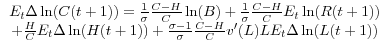
Under these assumptions, aggregate consumption growth is (approximately) given by the following equation

(9) $\begin{array}{c} E_t \Delta \ln (C(t+1))=(1-\varpi )\{\frac{1}{\sigma }\frac{C-H}{C}\ln (B)+\frac{1}{\sigma }\frac{C-H}{C}E_t \ln (R(t+1)) \ +\frac{H}{C}E_t A(L)\Delta \ln (C(t))+\frac{\sigma -1}{\sigma }\frac{C-H}{C}{v}'[L]LE_t \Delta \ln (L(t+1))\} \ +\varpi E_t \Delta \ln (Y(t+1)) \ \end{array}$

$\varpi$ is increasing in the share of rule-of-thumb consumers and decreasing in the share of property income in total household income (because such income does not accrue to rule-of-thumb households). The formula for the habit from equation 6, a distributed lag of consumption, has been substituted into equation 9.

4. Empirical results

Consumption, C(t), is measured by nondurable and services expenditures (excluding housing services) per capita. Our focus is on results using labor and transfer income per capita as the measure of Y(t). Labor supply, L(t), is measured by hours per capita in the nonfarm business sector. All growth rates are expressed at annual rates. The real interest rate, r(t), is the quarterly average of the three-month Treasury bill rate minus the (log) change in the personal consumption deflator over the previous four quarters.⁹ Parameter estimates are obtained via the Generalized Method of Moments (GMM). Finally, the habit process is assumed to depend simply on one lag of consumption.¹⁰

The following equation is estimated

(10) $\Delta \ln (C(t))=const.+sr(t)+h\Delta \ln (C(t-1))+l\Delta \ln (L(t))+b\Delta \ln (Y(t))+e(t)$ .

The parameters to be estimated are the constant, s, h, l, and b. In the absence of habit persistence, h equals zero. If preferences are separable between consumption and leisure, l equals zero. And b equals zero when rule-of-thumb behavior is not present.

The instrument set used in estimation consists of data lagged two periods or more, as time aggregation can induce first-order serial correlation in consumption growth (Working (1960)). In all cases, the instrument set includes the second and third lag of four variables: consumption growth, labor and transfer income growth, the real interest rate, and growth of hours per capita.

Table 2 reports the parameter estimates and tests of overidentifying restrictions. Panel A reports estimates for the period 1960:Q1 to 2004:Q4. Values of each parameter from an unrestricted version of equation 10 appear in the first column of numbers. Several results are apparent. First, only the coefficient on hours per capita - the parameter l associated with non-separable preferences between consumption and leisure/labor supply - is significant at the 10 percent level or better. Second, the standard errors of each parameter are fairly large. The latter result is not very surprising, as hours and labor income are correlated. Finally, the estimates do not support habit persistence, as the point estimate of the coefficient h is negative (and not significantly different from zero statistically).

As the results in the first column are not supportive of rule-of-thumb behavior and this is the most ad hoc hypothesis under consideration, the next two columns examine restricted specifications in which the coefficient b is set to zero. The second column of numbers considers both habit persistence and non-separable preferences between consumption and leisure/labor supply. The estimated value of the habit parameter h is negative and not statistically different from zero. In contrast, the estimated value of l is positive and statistically different from zero at the 1 percent level. The last column reports the estimates when both rule-of-thumb behavior and habit persistence are excluded (b and h equal to zero). The coefficient on hours per capita, l, equals about $\raise.5ex\hbox{$\scriptstyle 1$}\kern-.1em/ \kern-.15em\lower.25ex\hbox{$\scriptstyle 4$}$ and is statistically different than zero. The results provide support for non-separable preferences between consumption and leisure/labor supply and no support for habit persistence or rule-of-thumb behavior.

Panels B and C present parameter estimates for the same set of specifications for two sub-samples, 1960:Q1 to 1984:Q4 and 1985:Q1 to 2004:Q4. While the smaller samples appear to increase the standard errors of the parameter estimates, the results are essentially identical. The estimates indicate a significant coefficient on hours per capita in the consumption Euler equation, supporting non-separable preferences between consumption and leisure/labor supply. Moreover, the parameter estimate is stable at around $\raise.5ex\hbox{$\scriptstyle 1$}\kern-.1em/ \kern-.15em\lower.25ex\hbox{$\scriptstyle 4$}$ in both samples, as it should be if it reflects stable underlying preferences of households.

5. Summary

The predictability of consumption growth has posed a challenge to models of optimal consumer behavior since Hall's (1978) discovery that such models will typically imply that the change in marginal utility, and hence consumption growth, is unpredictable. This research adds to previous investigations by considering simultaneously a role for habit persistence, non-separable preferences between consumption and leisure/labor supply, and rule-of-thumb consumers. The data provided support for non-separable preferences between consumption and leisure/labor supply.

Data Appendix

Most series are taken directly from the Bureau of Economic Analysis's (BEA) National Income and Product Accounts (NIPA). The sample period used in estimation and in computing summary statistics is 1960:Q1 to 2004:Q4. Annualized growth rates from quarter-to-quarter are computed as 400 times the change in the natural logarithm of the variable.

Total consumption equals personal consumption expenditures in chain-weighted 2000 dollars (NIPA table 1.5.6, line 2).

Nondurables and services consumption excluding housing services equals total consumption minus durable expenditures and housing services in chain-weighted 2000 dollars (NIPA table 1.5.6, lines 3 and 13), where subtraction is performed via the Divisia approximation to the chain-weighting procedure followed by BEA.

Disposable personal income is taken from NIPA table 2.1, line 26. It is converted to real values by dividing by the personal consumption expenditure deflator (NIPA table 1.5.4, line 2).

Labor and transfer income equals compensation of employees received by persons minus contributions for government social insurance plus net transfers received by persons (NIPA table 2.1, line 2, minus NIPA tables 3.2 and 3.3, line 11, plus NIPA table 2.1, line 16, minus NIPA table 2.1, line 30) minus tax payments. Tax payments associated with labor and transfer income are computed as a portion of total personal income taxes equal to the share of labor income in labor and property income (i.e., transfer payments are assumed not to be taxed). Personal income taxes equal the sum of NIPA table 3.2, lines 3 and 10, and NIPA table 3.3, line 3.

The real interest rate equals the quarterly average yield on three-month U.S. Treasury bills (from the Federal Reserve Board's h.15 data release) minus the average of the annualized growth rate in the personal consumption deflator between the current quarter and four quarters earlier.

Hours are measured as hours worked in the nonfarm business sector from the Productivity and Cost release of the Bureau of Labor Statistics.

Population is measured by the civilian non-institutional population from the Employment Situation release of the Bureau of Labor Statistics.

References

Abel, Andrew B. (1990), "Asset Prices under Habit Formation and Catching Up with the Joneses." American Economic Review Papers and Proceedings, pp. 38-42.

Basu, Susanto and Miles Kimball (2002) "Long-Run Labor Supply and the Elasticity of Intertemporal Substitution for Consumption", Mimeo, University of Michigan at Ann Arbor, October.

Campbell, John Y., and Cochrane, John H. (1999), "By Force of Habit: A Consumption-Based Explanation of Aggregate Stock Market Behavior." The Journal of Political Economy, Vol. 107, No. 2, pp. 205-251.

Campbell, John Y. and Angus Deaton (1989) "Why is Consumption So Smooth?" Review of Economic Studies, vol. 56, pp. 357-374.

Campbell, John Y. and N. Gregory Mankiw (1989) "Consumption, Income and Interest Rates: Reinterpreting the Time Series Evidence," NBER Macroeconomics Annual, 4:185-216.

Campbell, John Y & Mankiw, N Gregory, 1990. "Permanent Income, Current Income, and Consumption," Journal of Business & Economic Statistics, vol. 8(3), pages 265-79.

Carroll, Christopher D. (2001), "Death to the Log-Linearized Consumption Euler Equation! (And Very Poor Health to the Second-Order Approximation)," Advances in Macroeconomics, 1(1), Article 6.

Carroll, Christopher D. and Martin Sommer (2003) Epidemiological Expectations and Consumption Dynamics. Mimeo.

Carroll, Christopher D., Jeffrey Fuhrer, and David Wilcox (1994) "Does consumer sentiment predict household spending? If so, why?", American Economic Review, 84, 1397-408.

Christiano, L., Eichenbaum, M. and C. Evans, (2005) "Nominal Rigidities and the Dynamic Effects of a Shock to Monetary Policy", Journal of Political EconomyFebruary, 113 (1), 1 -45.

Cochrane, John H. (1994) "Permanent and Transitory Components of GNP and Stock Prices," Quarterly Journal of Economics, vol. 109 (1), pp. 241-265.

Constantinides, George M. (1990) "Habit Formation: A Resolution of the Equity Premium Puzzle," Journal of Political Economy 98 (June 1990), 519-543.

Deaton, Angus (1992) Understanding Consumption, Oxford, Oxford University Press.

Dynan, Karen (2000) "Habit Formation in Consumer Preferences: Evidence from Panel Data," American Economic Review vol. 90 (June 2000), pp. 391-406.

Edge, Rochelle, Michael T. Kiley and Jean-Philippe Laforte (2007) "Natural Rate Measures in an Estimated DSGE Model of the U.S. Economy". Federal Reserve Board FEDS paper 2007-8 and forthcoming, Journal of Economic Dynamics and Control.

Ferson, Wayne E. and George M. Constantinides, (1991) "Habit persistence and durability in aggregate consumption: Empirical tests" Journal of Financial Economics, vol. 29, issue 2, pages 199-240.

Flavin, Marjorie. (1981), "The Adjustment of Consumption to Changing Expectations About Future Income." The Journal of Political Economy, Vol. 89, No. 5, pp. 974-1009.

Friedman, Milton (1957) A Theory of the Consumption Function, Princeton, Princeton University Press.

Fuhrer, Jeffrey C. (2000) "Habit Formation in Consumption and Its Implications for Monetary-Policy Models." American Economic Review, vol. 90, issue 3, pages 367-390

Gali, Jordi (1991) "Budget Constraints and Time Series Evidence on Consumption," American Economic Review, vol. 81, pp. 1238-1253.

Hall, Robert E. (1978) "Stochastic Implications of the Life Cycle-Permanent Income Hypothesis: Theory and Evidence," Journal of Political Economy, vol. 86, pp. 971-987.

Ravina, Enrichetta (2004) "Keeping Up With the Jones: Evidence from Micro Data." Mimeo, Northwestern University Department of Economics.

Ravn, Morten, Stephanie Schmitt-Grohe and Martin Uribe (2004) "Deep Habits." National Bureau of Economic Research Working Paper 10261.

Reis, Ricardo (2004) "Inattentive Consumers." National Bureau of Economic Research Working Paper 10883.

Tallarini, Thomas and Harold Zhang (2005) "External Habits and the Cyclicality of Expected Stock Returns." Journal of Business, 78:1023-48.

Working, Holbrook (1960) "Note on Correlation of First-Differences of Averages of a Random Chain", Econometrica, 28:916-918 (October).

Table 1: A Violation of the Permanent-income Hypothesis
Granger Causality Tests (1960:Q1 to 2004:Q4)
(null hypothesis: $\Delta$ ln(C) not predicted by lags of $\Delta$ ln(Y))
(p-value)
Measure of $\Delta$ ln(Y)	Measure of $\Delta$ ln(C) Nondurables and services	Measure of $\Delta$ ln(C) Total consumption
Labor and transfer income	0.033	0.011

Notes: Regressions include two lags of dependent variable and income measure.

Data: Nondurables and services is total consumption excluding purchases of durable goods and housing services. Total consumption is total consumption expenditures, including durable goods. Income is labor plus transfer income.

Source: Based on National Income and Product Accounts. The series for nondurables and services consumption and for labor and transfer income are taken from the Federal Reserve Board's FRB/US model database.

Table 2

Parameter Estimates

$\begin{displaymath} \Delta \ln (C(t))=const.+sr(t)+h\Delta \ln (C(t-1))+l\Delta \ln (L(t))+b\Delta \ln (Y(t))+e(t) \end{displaymath}$

Panel A: Sample period from 1960:Q1 to 2004:Q4
Coefficient: s	-.002 (.124)	-.001 (.148)	-.029 (.129)
Coefficient: h	-.142 (.266)	-.193 (.261)	-
Coefficient: l	*.222 (.123)	*******.313 (.116)	*******.257 (.092)
Coefficient: b	.289 (.231)	-	-
p-value for test of overidentifying restrictions	.718	.725	.652

Panel B: Sample period from 1960:Q1 to 1984:Q4
Coefficient: s	-.071 (.147)	-.046 (.212)	-.048 (.202)
Coefficient: h	.192 (.474)	-.060 (.311)	-
Coefficient: l	.079 (.282)	**.281 (.129)	**.264 (.112)
Coefficient: b	.299 (.385)	-	-
p-value for test of overidentifying restrictions	.697	.850	.881

Panel C: Sample period from 1985:Q1 to 2004:Q4
Coefficient: s	-.006 (.124)	-.004 (.121)	-.003 (.111)
Coefficient: h	-.168 (.328)	-.032 (.304)	-
Coefficient: l	*.319 (.174)	*.236 (.143)	**.226 (.105)
Coefficient: b	.083 (.141)	-	-
p-value for test of overidentifying restrictions	.371	.470	.613

Notes: *,**,*** denote statistically different from zero at the 10, 5, and 1 percent levels, respectively. Estimation by GMM using instruments discussed in text. Standard errors (in parentheses) corrected for heteroskedasticity and first-order autocorrelation.

Appendix: Additional results using alternative data and methods

This appendix contains estimation results analogous to those reported in the text for

Total personal consumption expenditures, rather than nondurable and services consumption excluding housing services (Table A1)
Disposable personal income, rather than after-tax labor and transfer income (Table A2)
Estimates obtained with a Fuller K estimator, rather than the GMM estimates (Table A3)

The results support the conclusion in the text. In particular, the data consistently suggest that the coefficient on hours worked in a consumption Euler equation is positive and significantly different from zero, while those on lagged consumption and contemporaneous income are not statistically different from zero and in some cases not of the correct sign to signal habit persistence or rule-of-thumb behavior. In other words, the data provide support for non-separable preferences between consumption and leisure/labor supply.

Table A1

Parameter Estimates using Total Consumption

$\begin{displaymath} \Delta \ln (C(t))=const.+sr(t)+h\Delta \ln (C(t-1))+l\Delta \ln (L(t))+b\Delta \ln (Y(t))+e(t) \end{displaymath}$

Panel A: Sample period from 1960:Q1 to 2004:Q4
Coefficient: s	-.163 (.144)	-.202 (.148)	-.212 (.142)
Coefficient: h	-.188 (.250)	-.139 (.237)	-
Coefficient: l	*.303 (.157)	.***422 (.150)	*******.381 (.122)
Coefficient: b	.464 (.356)	-	-
p-value for test of overidentifying restrictions	.419	.320	.349

Panel B: Sample period from 1960:Q1 to 1984:Q4
Coefficient: s	-.288 (.212)	-.305 (.233)	-.337 (.211)
Coefficient: h	-.231 (.256)	-.272 (.236)	-
Coefficient: l	*.447 (.248)	**.515 (.201)	**.395 (.159)
Coefficient: b	.116 (.300)	-	-
p-value for test of overidentifying restrictions	.388	.534	.445

Panel C: Sample period from 1985:Q1 to 2004:Q4
Coefficient: s	.008 (.146)	.009 (.138)	-.000 (.120)
Coefficient: h	-.218 (.280)	-.222 (.274)	-
Coefficient: l	*.404 (.214)	*.405 (.210)	**.330 (.152)
Coefficient: b	.005 (.152)	-	-
p-value for test of overidentifying restrictions	.079	.148	.209

Table A2

Parameter Estimates using Disposable Personal Income

$\begin{displaymath} \Delta \ln (C(t))=const.+sr(t)+h\Delta \ln (C(t-1))+l\Delta \ln (L(t))+b\Delta \ln (Y(t))+e(t) \end{displaymath}$

Panel A: Sample period from 1960:Q1 to 2004:Q4
Coefficient: s	-.056 (.127)
Coefficient: h	-.114 (.301)
Coefficient: l	**.207 (.103)
Coefficient: b	.224 (.153)
p-value for test of overidentifying restrictions	.597

Panel B: Sample period from 1960:Q1 to 1984:Q4
Coefficient: s	-.142 (.151)
Coefficient: h	.291 (.337)
Coefficient: l	.051 (.154)
Coefficient: b	.287 (.195)
p-value for test of overidentifying restrictions	.661

Panel C: Sample period from 1985:Q1 to 2004:Q4
Coefficient: s	.004 (.137)
Coefficient: h	-.256 (.506)
Coefficient: l	*.348 (.195)
Coefficient: b	.113 (.150)
p-value for test of overidentifying restrictions	.433

Table A3

Parameter Estimates using a Fuller-K estimator

$\begin{displaymath} \Delta \ln (C(t))=const.+sr(t)+h\Delta \ln (C(t-1))+l\Delta \ln (L(t))+b\Delta \ln (Y(t))+e(t) \end{displaymath}$

Panel A: Sample period from 1960:Q1 to 2004:Q4
Coefficient: s	-.005 (.119)	-.031 (.132)	-.032 (.127)
Coefficient: h	-.119 (.275)	-.167 (.310)	-
Coefficient: l	.222 (.143)	**.310 (.142)	*******.258 (.100)
Coefficient: b	.265 (.211)	-	-

Panel B: Sample period from 1960:Q1 to 1984:Q4
Coefficient: s	-.025 (.160)	-.016 (.190)	-.017 (.189)
Coefficient: h	.144 (.304)	-.002 (.337)	-
Coefficient: l	.112 (.194)	.278 (.170)	**.278 (.133)
Coefficient: b	.289 (.232)	-	-

Panel C: Sample period from 1985:Q1 to 2004:Q4
Coefficient: s	-.000 (.162)	-.039 (.157)	-.048 (.151)
Coefficient: h	-.188 (.403)	-.088 (.389)	-
Coefficient: l	*.369 (.190)	*.344 (.191)	*******.314 (.121)
Coefficient: b	.121 (.156)	-	-

Notes: *,**,*** denote statistically different from zero at the 10, 5, and 1 percent levels, respectively. Standard errors in parentheses. The Fuller constant is set to 4, implying K near 1.

Footnotes

1. * Address: Mail Stop 76, Federal Reserve Board, Washington, DC 20551. Email: [email protected]. I would like to thank participants at several workshops and especially Charles Fleischman, Andrew Levin, and David Wilcox for their comments on an earlier draft. Any remaining errors are the sole responsibility of the author. The views expressed herein are those of the author, and do not reflect the views of the Board of Governors of the Federal Reserve System or its staff. Return to Text

2. While clearly inspired by earlier work, rational-expectations versions of the permanent-income hypothesis differ significantly from the original work found in Friedman (1957). Return to Text

3. Another hypothesis is inattention by consumers (e.g., Carroll and Sommer (2003), Reis (2004)); this hypothesis is more difficult to test, as it involves potentially large delays between innovations in fundamentals and consumer responses, and such long delays imply that instrumental variable techniques used to estimate parameters and test alternative hypotheses may encounter severe problems because the lagged instruments may be quite weak. Future work should examine inattention more carefully. Return to Text

4. A large literature examines the asset pricing implications of habit persistence but does not examine the implications of habit persistence for consumption fluctuations per se; some representative examples include Constantinides (1990), Abel (1990), and Campbell and Cochrane (1999). There have also been some studies examining household-level data on consumption (e.g., Dynan (2000), Ravina (2004)). These household-level studies have reached mixed conclusions and are not well suited to addressing the range of alternative hypotheses considered herein (habits, non-separability, and rule-of-thumb behavior) because household-level data sets typically lack sufficient information on both consumption and income over long time periods. Return to Text

5. Carroll (2001) has criticized the focus on log-linear approximations, particularly for studies looking at household-level cross sections. As he notes, some of the biases he identifies are less likely to apply to time-series approaches or analyses of aggregate data. Return to Text

6. One caveat arises because the data refer to quarterly averages, which induce first-order serial correlation in the growth rate of a variable that is a random walk at higher frequencies (Working (1960)); the formal analysis in later sections will control for this complication. Return to Text

7. I have kept the discussion of previous work as short as possible. Other important contributions include Flavin (1981), who shows that consumption moves too closely with realized income (not permanent income), a finding termed excess sensitivity; Campbell and Mankiw (1989,1990) suggest that excess sensitivity reflects rule-of-thumb behavior; Campbell and Deaton (1989) show that consumption is too sensitive to per-period income flows (i.e., excess sensitivity) but also too insensitive to permanent income (i.e., excess smoothness); Gali (1991) also links excess smoothness and excess sensitivity; Cochrane (1994) presents evidence from vector-autoregressions that consumption growth is predictable and excessively smooth. Carroll, Fuhrer, and Wilcox (1994) show that survey measures of consumer sentiment predict consumption growth. Return to Text

8. The external habit assumption simplifies the analysis and is quite common (e.g., Abel (1990), Campbell and Cochrane (1999)). Return to Text

9. The approximate equality between the interest rate (r(t)) and the natural logarithm of the gross return (ln[R(t)]) has been used. Return to Text

10. An appendix provides estimates using total consumption instead of nondurables and services, considers disposable personal income rather than labor and transfer income, and contains results from k-class estimators that perform better than GMM in the presence of weak instruments. Return to Text

This version is optimized for use by screen readers. Descriptions for all mathematical expressions are provided in LaTex format. A printable pdf version is available. Return to Text