Documentation of the Research and Statistics Division's Estimated DSGE Model of the U.S. Economy: 2006 Version
Keywords: Two-sector growth model, sticky-prices, sticky-wages, habit-persistence, investment adjustment costs, variable utilization, Bayesian estimation
Abstract:
This paper provides documentation for the large-scale estimated DSGE model of the U.S. economy used in Edge, Kiley, and Laforte (2007). The model represents part of an ongoing research project (the Federal Reserve Board's Estimated, Dynamic, Optimization-based--FRB/EDO--model project) in the Macroeconomic and Quantitative Studies section of the Federal Reserve Board aimed at developing a DSGE model that can be used to address practical policy questions and the model documented here is the version that was current at the end of 2006. The paper discusses the model's specification, estimated parameters, and key properties.
This paper contains documentation for the large-scale estimated DSGE model of the U.S. economy that was employed in Edge, Kiley, and Laforte (2007) to discuss the use of DSGE models in a policy oriented environment. The model represents part of an ongoing research project in the Macroeconomic and Quantitative Studies section of the Federal Reserve Board aimed at developing a DSGE model that can be used to address practical policy questions. The outline of the paper is as follows. Section 1 provides a brief qualitative description of the model. Section 2 outlines the model's production, capital evolution, and preference technologies. Section 3 describes the economy's decentralization, and section 3 defines equilibrium in the model. Section 4 lists the data that is used in estimating the model. Section 5 reports the model's key estimation results, which include the estimated parameter values, variance decompositions, impulse response functions, and implied paths of model variables. The precise equations that characterize equilibrium in this model are contained in the appendix. Appendix A presents the equations of the symmetric model, appendix B reports the equations of the symmetric and stationary model, and appendix C gives the solution to the model's steady-state. Finally, since the model contains a large number of parameter and variable names a key is given in appendices D, E, and F.
Before moving to our presentation of the model, we note that we anticipate that the DSGE model developed in this paper (and subsequent versions of it) will serve as a complement to the analyses that are currently performed using existing large-scale econometric models, such as FRB/US model, as well as smaller, ad hoc models that we have found useful for more specific questions. Our model, while quite a bit more detailed and disaggregated than most existing DSGE models, is nonetheless incapable of addressing many of the questions addressed in a very large model like FRB/US and cannot therefore serve as the sole model for policy purposes. We suspect that model-based analyses are enhanced by consideration of multiple models (and, indeed, our experience suggests that often we learn as much when models disagree than when they agree). The use of multiple models will allow us to examine the robustness of policy strategies across models with quite different foundations, which we view as important given the significant divergences of opinion regarding the plausibility of various types of models.
1 Model Overview and Motivation
Figure 1 provides a graphical overview of the economy described by our model. The model possesses two final goods: slow-growing "CBI" goods--so called because most of these goods are used for consumption (C) and because they are produced by the business and institutions (BI) sector--and fast-growing "KB" goods--so called because these goods are used for capital (K) accumulation and are produced by the business (B) sector. The goods are produced in two stages by intermediate- and then final-goods producing firms (shown in the center of the figure). On the model's demand-side, there are four components of spending (each shown in a box surrounding the producers in the figure): consumer nondurable goods and services (sold to households), consumer durable goods, residential capital goods, and non-residential capital goods. Consumer nondurable goods and services and residential capital goods are purchased (by households and residential capital goods owners, respectively) from the first of economy's two final goods producing sectors (good CBI producers), while consumer durable goods and non-residential capital goods are purchased (by consumer durable and residential capital goods owners, respectively) from the second sector (good KB producers). We "decentralize" the economy by assuming that residential capital and consumer durables capital are rented to households while non-residential capital is rented to firms. In addition to consuming the nondurable goods and services that they purchase, households also supply labor to the intermediate goods-producing firms in both sectors of the economy.
Our assumption of a two-sector production structure is motivated by the trends in certain relative prices and categories of real expenditure apparent in the data. As reported in Table 1, expenditures on consumer non-durable goods and non-housing services and
residential investment have grown at roughly similar real rates of around 3-1/2 percent per year over the last 20 years, while real spending on consumer durable goods and on nonresidential investment have grown at around 6-1/2 percent per year. The relative price of residential investment
to consumer non-durable goods and non-housing services has been fairly stable over the last twenty years (increasing only 1/2 percent per year on average, with about half of this average increase accounted for by a large swing in relative prices over 2003 and 2004). In contrast, the prices of
both consumer durable goods and non-residential investment relative to those of consumer non-durable goods and non-housing services have decreased, on average, about 3 percent per year. A one-sector model is unable to deliver long-term growth and relative price movements that are consistent
with these stylized facts. As a result, we adopt a two-sector structure, with differential rates of technical progress across sectors. These different rates of technological progress induce secular relative price differentials, which in turn lead to different trend rates of growth across the
economy's expenditure and production aggregates. We assume that the output of the slower growing sector (denoted
![]() ) is used for consumer nondurable goods and services and residential capital goods and the output of a faster growing sector (denoted
) is used for consumer nondurable goods and services and residential capital goods and the output of a faster growing sector (denoted
![]() ) is used for consumer durable goods and non-residential capital goods, roughly capturing the long-run properties of the data summarized in Table 1.
) is used for consumer durable goods and non-residential capital goods, roughly capturing the long-run properties of the data summarized in Table 1.
The DSGE models of Christiano et al. [2005] and Smets and Wouters [2004] did not address differences in trend growth rates in spending aggregates and trending relative price measures, although an earlier literature--less closely tied to business cycle fluctuations in the data--did explore the multi-sector structure underlying U.S. growth and fluctuations.1 Subsequent models have adopted a multi-sector growth structure, including Altig et al. [2004], Edge, Laubach, and Williams [2003], and DiCecio [2005]; our model shares features with the latter two of these models.
The disaggregation of production (aggregate supply) leads naturally to some disaggregation of expenditures (aggregate demand). We move beyond a model with just two categories of (private domestic) final spending and disaggregate along the four categories of private expenditure mentioned earlier:
consumer non-durable goods and non-housing services (denoted
![]() ), consumer durable goods (denoted
), consumer durable goods (denoted
![]() ), residential investment (denoted
), residential investment (denoted ![]() ), and non-residential
investment (denoted
), and non-residential
investment (denoted
![]() ).
).
While differential trend growth rates are the primary motivation for our disaggregation of production, our specification of expenditure decisions is related to the well-known fact that the expenditure categories that we consider have different cyclical properties. As shown in Table 2, consumer durables and residential investment tend to lead GDP, while non-residential investment (and especially non-residential fixed investment, not shown) lags. These patterns suggest some differences in the short-run response of each series to structural shocks. One area where this is apparent is the response of each series to monetary-policy innovations. As documented by Bernanke and Gertler [1995], residential investment is the most responsive component of spending to monetary policy innovations, while outlays on consumer durable goods are also very responsive. According to Bernanke and Gertler [1995], non-residential investment is less sensitive to monetary policy shocks than other categories of capital goods spending, although it is more responsive than consumer nondurable goods and services spending.
Beyond the statistical motivation, our disaggregation of aggregate demand is motivated by the concerns of policymakers. A recent example relates to the divergent movements in household and business investment in the early stages of the U.S. expansion following the 2001 recession, a topic discussed in Kohn [2003]. We believe that providing a model that may explain the shifting pattern of spending through differential effects of monetary policy, technology, and preference shocks is a potentially important operational role for our disaggregated framework.
2 Production, Capital Evolution, and Preferences
In this section we present the production, capital evolution, and preference technologies for our model. The long-run evolution of the economy is determined by differential rates of stochastic growth in the production sectors of the economy; its short-run dynamics are influenced by various forms of adjustment costs. Adjustment costs to real aggregate variables are captured in the economy's preference, production, and capital evolution technologies presented in this section. Adjustment costs to real sectoral variables and nominal variables are captured in the decentralization of the model presented in the following section.
2.1 The Production Technology
As noted in the previous section our model economy produces two final goods and services: slow-growing "consumption" goods and services
![]() and fast-growing "capital" goods
and fast-growing "capital" goods
![]() . "Capital" goods are produced by businesses; "consumption" goods and services are produced by businesses and institutions. These final goods are produced by aggregating
(according to a Dixit-Stiglitz technology) an infinite number of differentiated inputs,
. "Capital" goods are produced by businesses; "consumption" goods and services are produced by businesses and institutions. These final goods are produced by aggregating
(according to a Dixit-Stiglitz technology) an infinite number of differentiated inputs,
![]() for
for ![]() , distributed over the unit interval. Specifically, final
goods production is governed by the function
, distributed over the unit interval. Specifically, final
goods production is governed by the function
The term
where
The ![]() th differentiated intermediate good in sector
th differentiated intermediate good in sector ![]() (which is used as an input
in equation 1) is produced by combining each variety of the economy's differentiated labor inputs
(which is used as an input
in equation 1) is produced by combining each variety of the economy's differentiated labor inputs
![]() with the sector's specific utilized non-residential capital stock
with the sector's specific utilized non-residential capital stock
![]() . (Utilized non-residential capital,
. (Utilized non-residential capital,
![]() , is equal to the product of physical non-residential capital,
, is equal to the product of physical non-residential capital,
![]() , and the utilization rate,
, and the utilization rate,
![]() ). A Dixit-Stiglitz aggregator characterizes the way in which differentiated labor inputs are combined to yield a composite bundle of labor, denoted
). A Dixit-Stiglitz aggregator characterizes the way in which differentiated labor inputs are combined to yield a composite bundle of labor, denoted
![]() . A Cobb-Douglas production function then characterizes how this composite bundle of labor is used with capital to produce--given the current level of multifactor productivity
. A Cobb-Douglas production function then characterizes how this composite bundle of labor is used with capital to produce--given the current level of multifactor productivity
![]() in the sector
in the sector ![]() --the intermediate good
--the intermediate good
![]() . The production of intermediate good
. The production of intermediate good ![]() is governed by the
function:
is governed by the
function:
and where we assume
where
The level of productivity in the capital goods producing sector has two components. The ![]() component represents an economy-wide productivity shock, while the
component represents an economy-wide productivity shock, while the
![]() term represents a productivity shock that is specific to the capital goods sector. The level of productivity in the consumption goods producing sector has only the one economy-wide
component,
term represents a productivity shock that is specific to the capital goods sector. The level of productivity in the consumption goods producing sector has only the one economy-wide
component, ![]() , since we assume
, since we assume
![]() . The exogenous productivity terms contain a unit root, that is, they exhibit permanent movements in their levels. We assume that the stochastic process
. The exogenous productivity terms contain a unit root, that is, they exhibit permanent movements in their levels. We assume that the stochastic process ![]() evolves according to
evolves according to
where
where
2.2 Capital Stock Evolution
As already noted, there are three types of physical capital stocks in our model economy: non-residential capital,
![]() , residential capital,
, residential capital, ![]() , and consumer durables capital,
, and consumer durables capital,
![]() .
.
Purchases of the economy's fast-growing "capital" good can be transformed into either non-residential capital,
![]() , which can be used to produce output in either sector of the economy, or into the economy's consumer-durable capital stock,
, which can be used to produce output in either sector of the economy, or into the economy's consumer-durable capital stock,
![]() , from which households derive utility. Purchases of the economy's slow-growing "consumption" good can be transformed into residential capital.
, from which households derive utility. Purchases of the economy's slow-growing "consumption" good can be transformed into residential capital.
The evolution of the economy's three capital stocks are given below in equations (8), (9), and (10). We assume that there is some stochastic element affecting the efficiency of investment--reflected in the term ![]() , for
, for ![]()
![]() and
and ![]() --in the capital accumulation process. These shocks are uncorrelated with each other and exhibit only transitory movements from their steady-state
unit mean.2 Letting
--in the capital accumulation process. These shocks are uncorrelated with each other and exhibit only transitory movements from their steady-state
unit mean.2 Letting
![]() denote the log-deviation of
denote the log-deviation of ![]() from its
steady-state value of unity, we assume that:
from its
steady-state value of unity, we assume that:
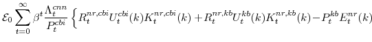
We also asssume that there are adjustment costs (captured by the final term in equations 8, 9, and 10) that are implied by capital installation. The evolution of capital is given by:
The parameter
2.3 Preferences
The ![]() th household derives utility from four sources: consumer non-durable goods and non-housing services,
th household derives utility from four sources: consumer non-durable goods and non-housing services,
![]() , the flow of services from consumer-durable capital,
, the flow of services from consumer-durable capital,
![]() , the flow of services from residential capital
, the flow of services from residential capital
![]() , and its leisure time, which is equal to what remains of its time endowment after
, and its leisure time, which is equal to what remains of its time endowment after
![]() hours are spent working. The preferences of household
hours are spent working. The preferences of household ![]() are separable over all of the arguments of its utility function. The utility that the household derives from the three components of its goods and services consumption is influenced by its habit stock for each of these consumption components, a feature that has been shown to be
important for consumption dynamics in similar models. Household
are separable over all of the arguments of its utility function. The utility that the household derives from the three components of its goods and services consumption is influenced by its habit stock for each of these consumption components, a feature that has been shown to be
important for consumption dynamics in similar models. Household ![]() 's habit stock for its consumption of non-durable goods and non-housing services, is equal to a factor
's habit stock for its consumption of non-durable goods and non-housing services, is equal to a factor ![]() multiplied by its consumption last period
multiplied by its consumption last period
![]() . The household's habit stock for its other components of consumption is defined similarly. In summary, the preferences of household
. The household's habit stock for its other components of consumption is defined similarly. In summary, the preferences of household ![]() are represented by the utility function:
are represented by the utility function:
The parameter
The variable
3 The Decentralized Economy
The economy's decentralization, which is also depicted in Figure 1, is as follows:
A representative firm in each of the economy's two final-goods producing sectors purchases intermediate inputs from the continuum of intermediate goods producers and produces the sector's final goods output.
Each firm in the economy's two intermediate-goods producing sectors rents non-residential capital from the capital owners and hires each type of differentiated labor from households so as to to produce its differentiated output. Because each firm is a monopolistically-competitive supplier of its own output, it is able to set the price at which it sells this output.
Each household purchases output from final-goods producers in the slow-growing "consumption" goods sector, which it then uses as non-durable goods and non-housing services, and rents consumer durables capital and residential capital from the capital owners. Because each household is a monopolistically-competitive supplier of its own labor, it is able to set the wage at which it supplies its labor services.
Each non-residential and consumer durables capital owner purchases output from the fast-growing "capital" final-goods sector and transforms it into either non-residential or consumer durables capital. Each residential capital owner purchases output from the slow-growing "consumption" final-goods and transforms it into residential capital.
The monetary authority sets the nominal interest rate given an interest rate feedback rule with smoothing of the policy response to endogenous variables.
The government and foreign economic agents demand a share of the economy's output.
We describe in this section the behaviour of agents listed above.
3.1 Consumption and Capital Final Goods Producers
The representative, perfectly competitive firm in the final consumption good sector owns the production technology described in equation (1) for ![]() , while the
representative, perfectly competitive firm in the final capital goods sector owns the same technology for
, while the
representative, perfectly competitive firm in the final capital goods sector owns the same technology for ![]() . The final-good producer in sector
. The final-good producer in sector ![]() solves the cost-minimization problem of:
solves the cost-minimization problem of:
3.2 Consumption and Capital Intermediate Goods Producers
Each intermediate-good producing firm
![]() and
and ![]() owns the production technology described in
equation (3). It is convenient to think of the intermediate good producing firm as solving three problems: two factor-input cost-minimization problems and one price-setting profit-maximization problem. The two cost-minimization problems faced by the representative
firm in sector s are:
owns the production technology described in
equation (3). It is convenient to think of the intermediate good producing firm as solving three problems: two factor-input cost-minimization problems and one price-setting profit-maximization problem. The two cost-minimization problems faced by the representative
firm in sector s are:
and
The profit-maximization problem faces by the firm is given by:
The variable
3.3 Capital Owners
Capital owners possess the technologies described in equations (8) and (9) for transforming the economy's fast-growing "capital" good into either non-residential capital,
![]() , or the consumer-durable capital stock,
, or the consumer-durable capital stock,
![]() , and in equation (10) for transforming the economy's slow-growing "consumption" good into the economy's residential capital stock
, and in equation (10) for transforming the economy's slow-growing "consumption" good into the economy's residential capital stock
![]() .
.
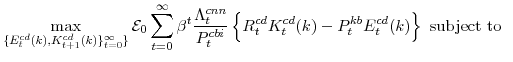
The non-residential capital owner solves:
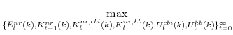

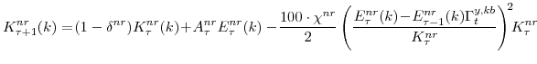
We assume that the capital owner decides on both the amount of capital that it will rent to firms and the rate of utilization at which this capital is used by firms. (Recall that the firm's choice variable in 15 is utilized capital
while the residential capital owner solves:
3.4 Households
The household possesses the utility function--defined over three components of goods and services consumption and leisure--described by equation (11).The representative household solves the problem:


The household's budget constraint incorporates wage setting adjustment costs (the size of which depend on the parameter
3.5 Market Clearing
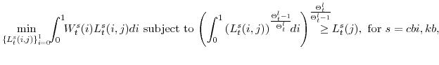
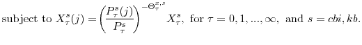
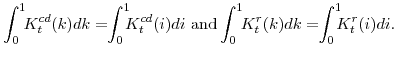
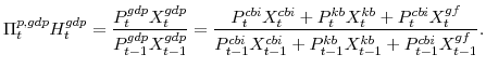
There are a number of market clearing conditions that must be satisfied in our model. Market clearing in the slow-growing "consumption" goods and fast-growing "capital" goods sectors, given price- and wage-adjustment costs and variable utilization costs implies that

and
The market clearing conditions for the labor and non-residential capital supplied and demanded in sector
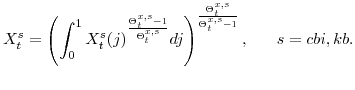
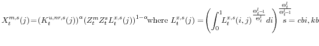
![\displaystyle L^{s}_{t}(i)=\!\!\int_{0}^{1}\!\!\!L^{s}_{t}(i,j)dj {\mathrm{and}} \!\!\int_{0}^{1}\!\!U(k)^{s}_{t}K^{nr,s}_{t}(k)dk=\!\!\int_{0}^{1}\!\!\!K^{u,nr,s}_{t}(j)dj \forall i \in [0,1] {\mathrm{and for}} s=cbi,kb.](img139.gif)
The market clearing conditions for consumer durables and residential capital are
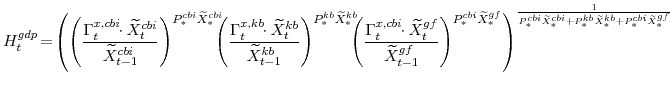
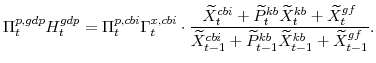
3.7 Real GDP Growth and GDP Price Inflation
Real GDP growth and the inflation rate of the GDP deflator are two variables of interest to policy-makers that do not automatically appear in our model. Real GDP growth is constructed as the divisia (share-weighted) aggregate of output in the economy, that is:
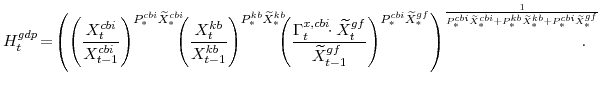
To a first-order approximation, this definition of GDP growth is equivalent to how it is defined in the U.S. NIPA. The variable
3.8 Monetary Authority
The central bank sets monetary policy in accordance with a Taylor-type interest-rate feedback rule. Policymakers smoothly adjust the actual interest rate ![]() to its target level
to its target level
![]()
where the parameter

where
4 Equilibrium
Before characterizing equilibrium in this model, we define three additional variables, the price of installed non-residential capital
![]() , the price of installed consumer durables capital
, the price of installed consumer durables capital
![]() , and the price of installed residential capital
, and the price of installed residential capital
![]() . These variables are the lagrange multiplier on the capital evolution equations that would be implied by the
. These variables are the lagrange multiplier on the capital evolution equations that would be implied by the ![]() th capital owner's profit-maximization problems (described in equations 17, 18, and 19).
th capital owner's profit-maximization problems (described in equations 17, 18, and 19).
Equilibrium in our model is an allocation:
and a sequence of values
|
|||

|
that satisfy the following conditions:
- The model's two representative final-good producing firms solve (13) for
 and
and  ;
; - All intermediate-good producers
![j \in [0,1]](img100.gif) solve (14), (15), and (16) for and ;
solve (14), (15), and (16) for and ; - All capital owners
![k \in [0,1]](img176.gif) solve (17), (18), and (19);
solve (17), (18), and (19); - All households
![i \in [0,1]](img177.gif) solve (20);
solve (20); - The two final goods markets clear as in (22) and (23);
- All intermediate goods markets clear (by construction);
- The labor and non-residential capital markets clear as in (24);
- The consumer durable and residential capital rental markets clear as in (25);
- The identities given in (26) hold, but are modified slightly to
![\displaystyle \frac{W^{s}_{t}(i)}{P^{c}_{t}} =\frac{\Pi^{w,s}_{t}(i)}{\Pi^{p,c}_{t}}\cdot \frac{W^{s}_{t-1}(i)}{P^{c}_{t-1}} \mathrm{and} \frac{W^{s}_{t}}{P^{c}_{t}} =\frac{\Pi^{w,s}_{t}}{\Pi^{p,c}_{t}}\cdot \frac{W^{s}_{t-1}}{P^{c}_{t-1}} {\mathrm{for all}} i \in [0,1] {\mathrm{and for}} s=cbi,kb;](img178.gif)
- The identities given in (27) hold, although are modified slightly to
![\displaystyle \frac{P^{s}_{t}(j)}{P^{c}_{t}} =\frac{\Pi^{p,s}_{t}(j)}{\Pi^{p,c}_{t}}\cdot\frac{P^{s}_{t-1}(j)}{P^{c}_{t-1}} \mathrm{and} \frac{P^{k}_{t}}{P^{c}_{t}} =\frac{\Pi^{p,k}_{t}}{\Pi^{p,c}_{t}}\cdot\frac{P^{k}_{t-1}}{P^{c}_{t-1}} {\mathrm{for all}} j \in [0,1] {\mathrm{and for}} s=cbi,kb;](img179.gif)
- The monetary authority follows (30) and (31), where the growth rate of GDP and aggregate prices are defined by equations (28) and (29).
5 Data
The model is estimated using 11 data series listed below. Except where noted, the series are from the U.S. National Income and Product Accounts (U.S. NIPA) published by the Bureau of Economic Analysis.
- Nominal gross domestic product.
- Nominal consumption expenditures on non-durables and non-housing services.
- Nominal consumption expenditure on durables.
- Nominal residential investment expenditure.
- Nominal business investment expenditure (which equals nominal gross private domestic investment minus nominal residential investment and thus includes inventory investment).
- The rate of GDP price inflation.
- The rate of inflation for prices of consumer non-durables and non-housing services (which represents inflation in the slow-growing "consumption" goods sector).
- The rate of inflation for prices of consumer durables (which represents inflation in the fast-growing "capital" goods sector).
- Hours, which equals hours of all persons in the non-farm business sector (from the Bureau of Labor Statistics) scaled up by the ratio of nominal production in our model to nominal non-farm business sector output.4
- Wage inflation, which equals compensation per hour in the non-farm business sector (from the Bureau of Labor Statistics).
- The federal funds rate (from the Federal Reserve Board).
Some of the series are not those used in previous research with the Federal Reserve's FRB/US model. However, price and nominal quantity indices for each of the model's expenditure and output variables can be retrieved easily from the U.S. NIPA. The construction of these series are as follows:
Nominal expenditures on consumer non-durable goods and non-housing services (
![]() ) is the sum of nominal personal consumption expenditures on non-durable goods and nominal personal consumption expenditures on services (Table 1.1 of the NIPA) with
owner-occupied nonfarm dwellings and tenant-occupied nonfarm dwellings (Table 2.4) subtracted.
) is the sum of nominal personal consumption expenditures on non-durable goods and nominal personal consumption expenditures on services (Table 1.1 of the NIPA) with
owner-occupied nonfarm dwellings and tenant-occupied nonfarm dwellings (Table 2.4) subtracted.
Nominal expenditures on consumer durable goods (
![]() ) is nominal personal consumption expenditures on durable goods (Table 1.1).
) is nominal personal consumption expenditures on durable goods (Table 1.1).
Nominal expenditures on residential investment (![]() ) is nominal gross private domestic residential investment (Table 1.1).
) is nominal gross private domestic residential investment (Table 1.1).
Nominal expenditures on non-residential investment (
![]() ) is the sum of nominal gross private domestic non-residential investment and the change in nominal private inventories (Table 1.1).
) is the sum of nominal gross private domestic non-residential investment and the change in nominal private inventories (Table 1.1).
Nominal production in the slow-growing part of the business and institutions sector (
![]() ) is the sum of nominal expenditures on consumer non-durable goods and non-housing services (
) is the sum of nominal expenditures on consumer non-durable goods and non-housing services (
![]() ) and nominal expenditures on residential investment (
) and nominal expenditures on residential investment (![]() ).
).
Nominal production in the fast-growing part of the business sector (
![]() ) is the sum of nominal expenditures on consumer durable goods (
) is the sum of nominal expenditures on consumer durable goods (
![]() ) and nominal expenditures on non-residential investment (
) and nominal expenditures on non-residential investment (
![]() ).
).
In summary,
In the NIPA, there is a different price index for every expenditure and output variable. Our theoretical model has only one price per output good.5
To bring our data in line with our model the series must be modified slightly. Although the three price indices ![]() ,
, ![]() , and
, and ![]() are not identical they do not display any dramatic relative price swings. Similarly, the indicies
are not identical they do not display any dramatic relative price swings. Similarly, the indicies ![]() ,
, ![]() , and
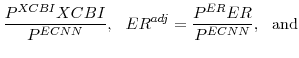
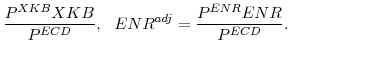
, and ![]() , while not identical, do not exhibit any large swings. Consequently, we make the following modification to the data. We re-write equations (32) and (33) as
, while not identical, do not exhibit any large swings. Consequently, we make the following modification to the data. We re-write equations (32) and (33) as
![\displaystyle P^{ECNN}\left[\frac{P^{XCBI}XCBI}{P^{ECNN}}\right]](img204.gif) |
![\displaystyle P^{ECNN}ECNN + P^{ECNN}\left[\frac{P^{ER}ER}{P^{ECNN}}\right], \mathrm{and}](img205.gif) |
||
![\displaystyle P^{ECD}\left[\frac{P^{XKB}XKB}{P^{ECD}}\right]](img206.gif) |
![\displaystyle P^{ECD}ECD + P^{ECD}\left[\frac{P^{ENR}ENR}{P^{ECD}}\right] ,](img207.gif) |
 |
|||
 |
Equations (32) and (33) can then be written as:
The above renormalization of the data implies that the series for real expenditures on residential investment (
Our decision for choosing the price index of consumer non-durables and non-housing services as our price index for the slow-growing sector and the price index of consumer durables as our price index for the fast-growing sector is that the PCE price deflator is ultimately the price index that we are most interested in from a policy perspective. Consequently, it is the components of this index that we wish to model.
6.1 Estimation
We take a log-linear approximation to our model, cast this resulting dynamical system in its state space representation for the set of (in our case 11) observable variables, use the Kalman filter to evaluate the likelihood of the observed variables, and form the posterior distribution of the parameters of interest by combining the likelihood function with a joint density characterizing some prior beliefs. Since we do not have a closed-form solution of the posterior, we rely on Markov-Chain Monte Carlo (MCMC) methods.
We add measurement errors processes, denoted ![]() , for all of the observed series used in estimation except the nominal interest rate and the aggregate hours series. The measurement
errors explain less than 5 percent of the observed series.6
, for all of the observed series used in estimation except the nominal interest rate and the aggregate hours series. The measurement
errors explain less than 5 percent of the observed series.6
6.2 Model Parameters
The model' calibrated parameters are presented in Table 3, while the estimated parameters are presented in Tables 4 and 5. We based out decision on which parameters to calibrate and which to estimate on how informative the data were likely to be on the parameter, as well as identification and overparameterization issues. The first three columns of Table 4 and 5 outline our assumptions about the prior distributions of the estimated parameters, the remaining columns describe the parameters' posterior distributions, which we now proceed to discuss.
We consider first the parameters related to household-spending decisions. The parameters related to habit-persistence are uniformly large. For nondurables and services excluding housing, the habit parameter is about 0.8, close to the value in found by Fuhrer [2000]. For consumer durables capital the habit parameter is somewhat smaller, while for residential capital it is smaller still. Since most DSGE models do not consider utility functions with this level of disaggregation, there is little consensus on these values. In addition, simulations indicate that habit and adjustment cost parameters--both present in our model--are closely related, further complicating any comparison. Indeed, we estimate investment adjustment costs to be very significant for residential investment but of modest importance for consumer durables.7 Nonetheless, habit-persistence and investment adjustment costs are important in generating "hump-shaped" responses of these series to monetary policy shocks.8 The estimated value of the remaining preference parameter, the inverse of the labor supply elasticity, is, at a bit over one, a little higher than suggested by the balance of microeconomic evidence (see Abowd and Card [1989]).
With regard to adjustment cost parameters for non-residential investment, we estimate significant costs to the change in investment flows, which imply an elasticity of investment to marginal q of about 1/3. We also find an important role for the sectoral adjustment costs to labor: In our multisector setup, shocks to productivity or preferences in one sector of the economy result in strong shifts of labor towards that sector, which conflicts with the high degree of sectoral co-movement in the data. The adjustment costs to the sectoral mix of labor input ameliorate this potential problem, as in Boldrin et al. [2001].
Finally, adjustment costs to prices and wages are both estimated to be important, although prices appear "stickier" than wages. Our quadratic costs of price and wage adjustment can be translated into frequencies of adjustment consistent with the Calvo model; these are about six quarters for prices and about one quarter for wages. However, these estimates are very sensitive to the specifics of our model and would be altered by reasonable assumptions regarding "real rigidities" such as firm-specific factors or "kinked" demand curves. We find only a modest role for lagged inflation in our adjustment cost specification (around 1/3), equivalent to modest indexation to lagged inflation in other sticky-price specifications. This differs from some other estimates, perhaps because of the focus on a more recent post-1983 sample (similar to results in Kiley [2007] and Laforte [2007]).
6.3 Variance Decompositions
Tables 6 to 11 present forecast error variance decompositions at various (quarterly) horizons at the posterior mode of the parameter estimates for key variables and shocks. We run through the key results here.
Volatility in aggregate GDP growth is, in the near horizon, accounted for predominantly by economy-wide technology shocks, non-residential investment efficiency shocks, and exogenous spending shocks. In the far horizon, volatility is accounted for primarily by capital-specific and economy-wide technology shocks.
Volatility in GDP price inflation is, in the near horizon, accounted for by mark-up shocks in the slow-growing (CBI) sector and economy-wide and capital-specific technology shocks. In the far horizon, its volatility is accounted for by economy-wide and capital-specific technology shocks.
Volatility in the nominal interest rate is, in the near horizon, accounted for primarily by shocks in the policy rule, non-residential investment efficiency shocks, exogenous spending shocks, and mark-up shocks in the slow-growing (CBI) sector. In the far horizon, its volatility is accounted for by non-residential investment efficiency shocks and to a much lesser extent consumption preference shocks.
Volatility in expenditures on consumer non-durables and non-housing services is, in the near horizon, accounted for predominantly by economy-wide technology shocks and to a lesser extent its own preference shock. In the far horizon, volatility is accounted for primarily by capital-specific and economy-wide technology shocks, and non-residential investment efficiency shocks.
Volatility in expenditures on consumer durables is, in the near horizon, accounted for predominantly by non-residential investment efficiency shocks, and its own preference and investment efficiency shocks. In the far horizon, its volatility is accounted for primarily by capital-specific and non-residential investment efficiency shocks.
Volatility in expenditures on residential investment is, in the near horizon, accounted for predominantly by its own investment efficiency shocks. In the far horizon, its volatility is accounted for primarily by non-residential investment efficiency shocks and to a lesser extend economy-wide and capital-specific technology shocks.
Volatility in expenditures on non-residential investment is, in both the near and far horizon, accounted for almost exclusively by non-residential investment efficiency shocks.
Volatility in hours is, in the near horizon, accounted for primarily by economy-wide technology shocks and non-residential investment efficiency shocks. In the far horizon, its volatility is accounted for by labor supply shocks.
Volatility in wage inflation is, in the near horizon, accounted for primarily by mark-up shocks in the labor market and labor supply shocks. In the far horizon, its volatility is accounted for by non-residential investment efficiency shocks and economy-wide and capital specific technology shocks.
Volatility in price inflation in the slow-growing part of the business and institutions sector is, in the near horizon, accounted for primarily by mark-up shocks in its sector and to a lesser extent economy-wide technology shocks. In the far horizon, its volatility is accounted for by economy-wide and non-residential investment efficiency shocks.
Volatility in price inflation in the fast-growing part of the business sector is, in the near horizon, accounted for primarily by mark-up shocks in its sector and captial specific technology shocks. In the far horizon, its volatility is accounted for by economy-wide technology shocks and non-residential investment efficiency shocks.
Overall, technology shocks and non-residential investment efficiency shocks seem to be the most important in accounting for the volatility of the data. Notably, economy-wide technology shocks account for a significant portion of the variability of nondurable and nonhousing services consumption (as well as aggregate GDP), while non-residential investment efficiency shocks account for a sizeable share of the variability of both durables consumption and non-residential investment (as well as aggregate GDP). As a result our estimated model is able to deliver co-movement between expenditure expenditure categories and production aggregates despite the present of a large number of expenditure specific expenditure-specific household preference shocks and capital-specific efficiency shocks, which by themselves typically create problems for the model in matching the co-movement properties of the data.
6.4 Impulse Responses
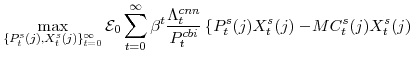
Figures 2 to 15 present the impulse responses of key variables to the models four preference shocks (
![]() ,
,
![]() ,
,
![]() , and
, and
![]() ), four capital efficiency shocks (
), four capital efficiency shocks (
![]() ,
,
![]() , and
, and ![]() ), the autonomous spending shock (
), the autonomous spending shock (![]() ), mark-up shocks (
), mark-up shocks (
![]() and
and
![]() ), technology shocks (
), technology shocks (
![]() and
and
![]() ), and monetary policy shock (
), and monetary policy shock (
![]() ).
).
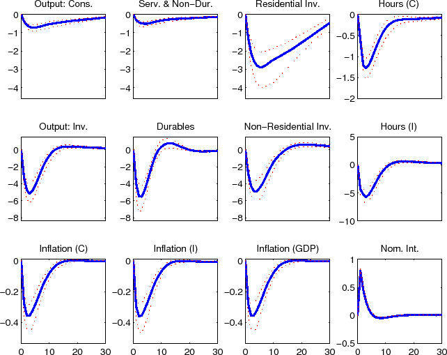
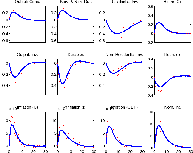
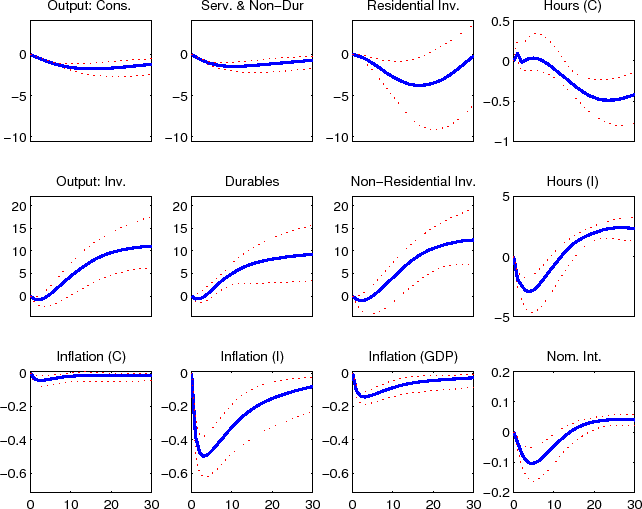
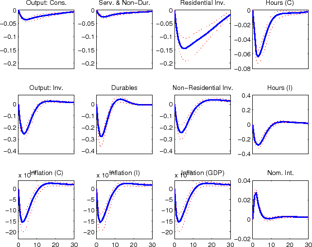
The impulse responses to a monetary policy innovation (shown in figure 2) captures the conventional wisdom regarding the effects of such shocks. In particular, both household and business expenditures on durables (consumer durables, residential investment, and nonresidential investment) respond strongly (and with a hump-shape) to a contractionary policy shock, with more muted responses by nondurables and services consumption; each measure of inflation responds gradually, albeit probably more quickly than in some analyses based on vector autoregressions.
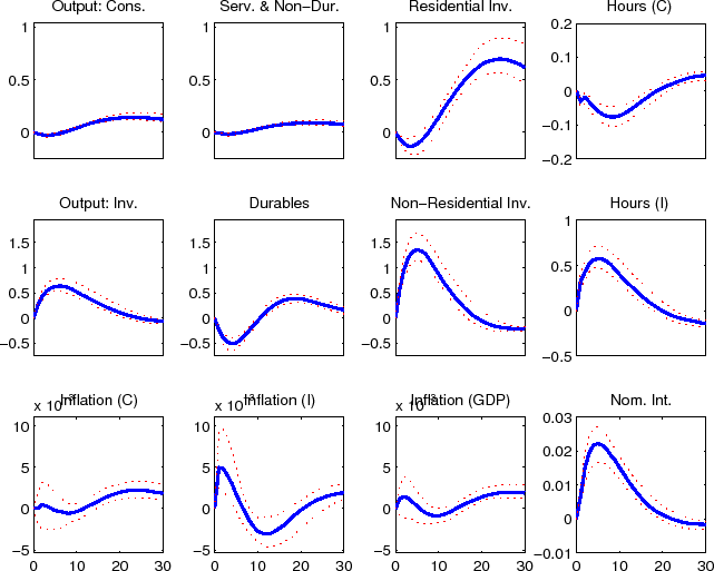
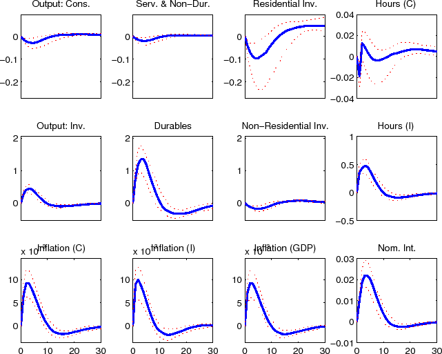
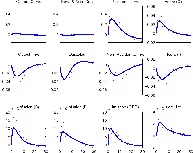
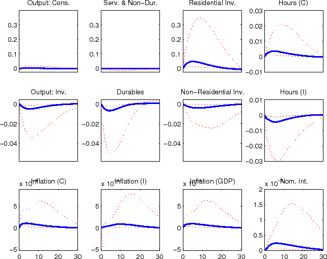
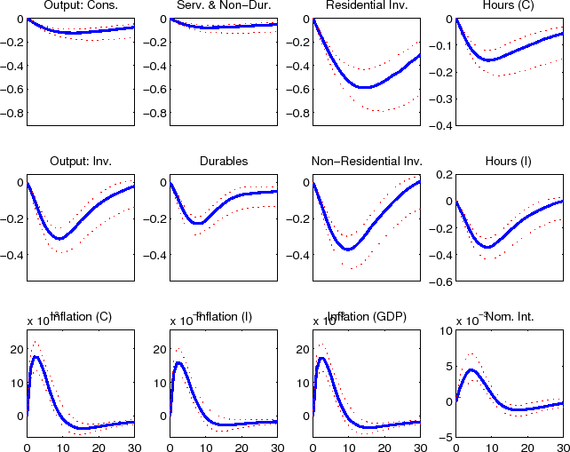
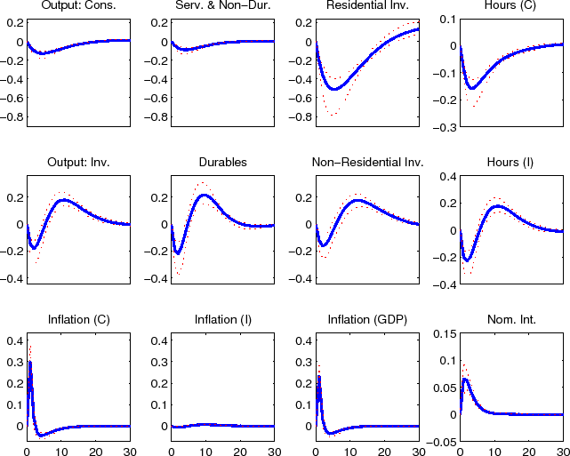
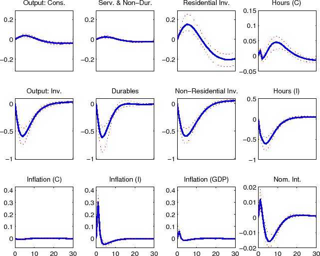
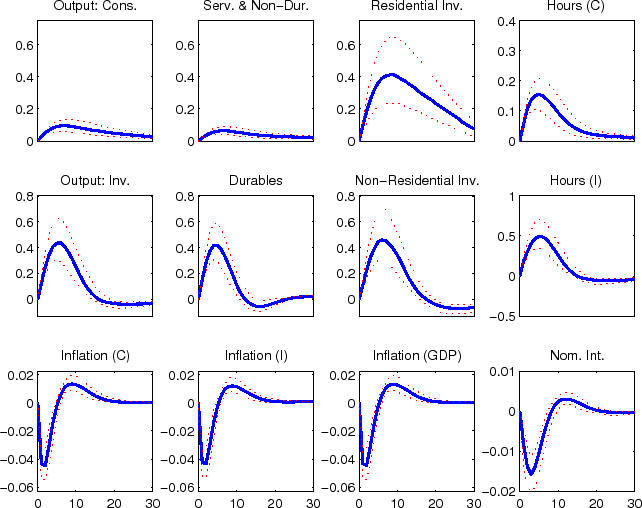
The impulse responses to a non-residential investment efficiency shock (shown in figure 3) boosts non-residential investment, initially at the expense of other investment expenditures. Consumption spending does not decline initially, but rather remains flat, reflecting household's expectation of higher levels of future output and consumption smoothing. After non-residential investment spending has been put in place and the economy's capital stock has expanded all components of spending rise above their steady-state level. The initial counter movements in investment spending is a result that is typically associated with expenditure specific shocks. The fact that non-residential investment adds to the economy's productive capactiy is the only reason that these opposing movements do not remain in the longer term. For example, the economy's other investment specific efficiency shocks for consumer durables and residential (shown in figures 4 and 5) lead to opposing movements in expenditure over the full duration of the effects of the shock; this is also the case for the economy's consumer non-durables and non-housing services and residential preference shocks (shown in figures 6 and 8). The consumer durables preference shock (shown in figures 7) displays some immediate co-movement although later the opposing movements in expenditures re-emerge. Naturally, the labor supply preference shock leads to co-movement between expenditure categories (see figure 9), although ultimately, as was evident from the variance decomposition results, this shock accounts for relatively little variation in these data.
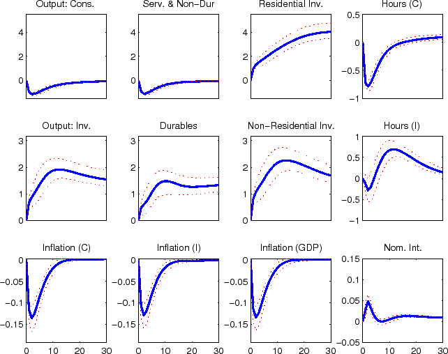
The impulse responses to an economy-wide technology shock (shown in figure 10), reflect the typical non-residential capital deepending effects associated with such a shock. Hours in the fast-growing (KB) sector falls in the near term in response to the shock, since the increase in labor productivity exceeds the sluggish increase in demand for goods in this sector. Hours fall in the slow-growing (CBI) sector in response to the slow increase in consumption demand.
The impulse responses to a capital-specific technology shock (shown in figure 11), also reflects non-residential capital deepending, although this takes place with some delay. The delay reflects the very persistent nature of capital-specific technology shocks, which leads firms to expect an extended period of strong capital-specific technology shocks and therefore expect future price declines. This raises the real interest rate relevant to non-residential investment, which slows the initial response despite the decline in the relative price of non-residential investment goods.
6.5 Implied Paths
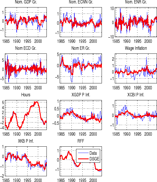
Figure 16 compares the one-step ahead DSGE model forecast to the actual observations for the data. These indicate that that the model has reasonable success in tracking fluctuations in most series.
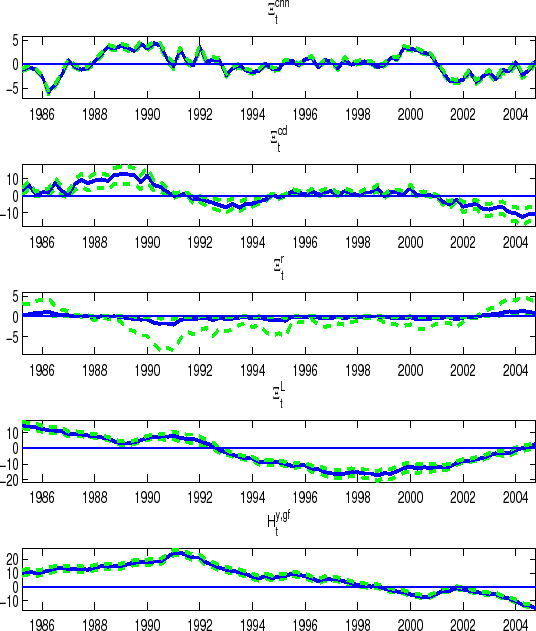
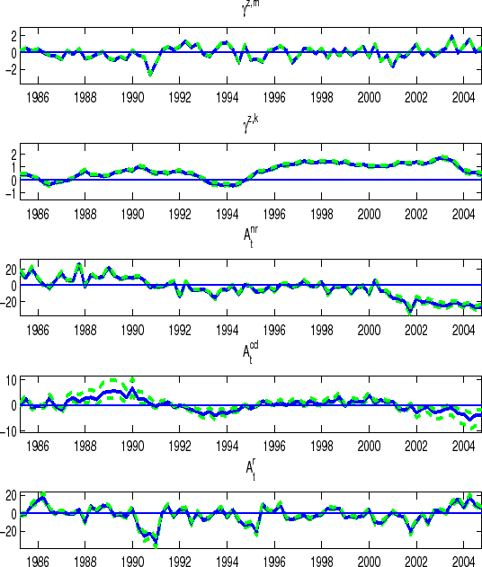
Figures 17 and 18 reports on the model's structural shocks implied by estimation; showing the median and the 95 percent credible set of the smoothed paths of these shocks. The paths of these shocks over the model's estimation period
provides us with an structural interpretation of the factors underlying recent macroeconomic phenomena. For example, the estimated paths of ![]() and
and ![]() , the stochastic variables that multiply the utility derived from non-durable goods and non-housing services consumption and durable goods consumption (shown in the top two panels of figure 17) dropped sharply in late 1990 and early 1991. That is, at this time, for a given level of wealth, income, and habits, households desired to consume less. One explanation for this seemingly exogenous desire to consume less is a decline in consumer confidence, which is one of the
widely accepted accounts for the 1990-91 recession. Note also that economy-wide technology growth,
, the stochastic variables that multiply the utility derived from non-durable goods and non-housing services consumption and durable goods consumption (shown in the top two panels of figure 17) dropped sharply in late 1990 and early 1991. That is, at this time, for a given level of wealth, income, and habits, households desired to consume less. One explanation for this seemingly exogenous desire to consume less is a decline in consumer confidence, which is one of the
widely accepted accounts for the 1990-91 recession. Note also that economy-wide technology growth,
![]() (shown in the top panel of figure 18) also dropped sharply in late 1990, consistent with a more traditional RBC interpretation of the recession.
(shown in the top panel of figure 18) also dropped sharply in late 1990, consistent with a more traditional RBC interpretation of the recession.
The model attributes the U.S. economy's exceptional performance in the second half of the 1990s to a sustained episode of well-above average investment-specific technology growth,
![]() (shown in the second panel of figure 18) as well as a extended sequence of favorable labor supply shocks,
(shown in the second panel of figure 18) as well as a extended sequence of favorable labor supply shocks, ![]() (shown in the second to last panel of figure 17). The rapid advances made in the 1990s in the production of high-tech investment and consumer durable goods is well documented and is accepted as
one of the reasons why the U.S. economy was able to grow at so fast a rate over this period while generating relatively little inflation. The explanation for the 1990s phenomena based on a long sequence of favorable labor supply shocks is somewhat less appealing since it ultimately just reflects
the fact that over this period it was possible to induce households to supply more labor without their demanding the higher rates of compensation that they typically would. Clearly, it would be more interesting to understand why this was the case.
(shown in the second to last panel of figure 17). The rapid advances made in the 1990s in the production of high-tech investment and consumer durable goods is well documented and is accepted as
one of the reasons why the U.S. economy was able to grow at so fast a rate over this period while generating relatively little inflation. The explanation for the 1990s phenomena based on a long sequence of favorable labor supply shocks is somewhat less appealing since it ultimately just reflects
the fact that over this period it was possible to induce households to supply more labor without their demanding the higher rates of compensation that they typically would. Clearly, it would be more interesting to understand why this was the case.
Finally, the model attributes the 2001 recession to an adverse consumer confidence shock--albeit mostly in non-durable goods and non-housing services consumption, ![]() --and a
unfavorable shock to business investment spending,
--and a
unfavorable shock to business investment spending, ![]() (shown in the middle panel of figure 18), which made business capital accumulation appear less
attractive that would typically be the case given underlying fundamentals. Again, the DSGE model's view of the 2001 recession does not seem inconsistent with alternatively derived interpretations. Note also, that the unfavorable shock to business investment expenditures,
(shown in the middle panel of figure 18), which made business capital accumulation appear less
attractive that would typically be the case given underlying fundamentals. Again, the DSGE model's view of the 2001 recession does not seem inconsistent with alternatively derived interpretations. Note also, that the unfavorable shock to business investment expenditures, ![]() , persists beyond the 2001 recession, possibly reflecting the effects of geo-political risks and corporate scandals that continued to restrain spending through the early years of the recovery.
, persists beyond the 2001 recession, possibly reflecting the effects of geo-political risks and corporate scandals that continued to restrain spending through the early years of the recovery.
7 Summing up
This paper has presented documentation for the large-scale estimated DSGE model of the U.S. economy used in Edge, Kiley, and Laforte (2007), which is being developed as part of an ongoing research project in the Macroeconomic and Quantitative Studies section of the Federal Reserve Board aimed at developing a DSGE model that can be used to address practical policy questions. Since our work on this model is ongoing, refinements to the model presented in this paper will very likely take place at future dates; at such time, revised documentation will be made available to interested readers.
A. The Symmetric Equilibrium
The symmetric equilibrium is an allocation:
and a sequence of values
 |
|||
|
that satisfy the symmetric versions of the first order conditions implied by:
- The intermediate-good producers' second cost-minimization problem (described in 15) and profit-maximization problem (described in 16);
- The capital owners' profit-maximization problems (described in 17, 18, and 19); and
- The households' utility maximization problems (described in 20);
- The model's market clearing conditions of which only the following need to be explicitly included:

- The identities between real wages, relative prices, and wage and price inflation rates:
- Equations (30) and (31) that describe the behavior of monetary policy; and
- Equations (28), and (29) that define the growth rate of the GDP aggregate and price index.
The symmetric first-order conditions implied by the second step of the intermediate-goods producing firms' cost minimization problems (equation 15) are:
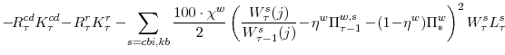
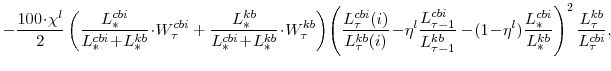
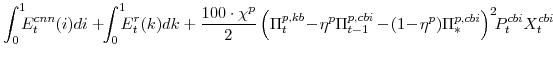
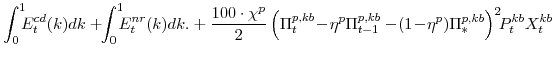
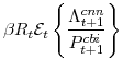
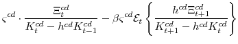
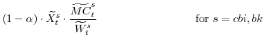
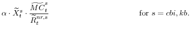
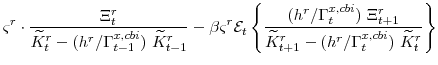
The key equation from the intermediate-goods producing firms' profit maximization problems (equation 16) are the price Phillips curves
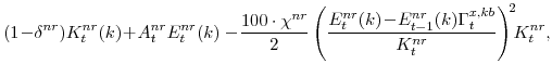
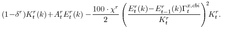
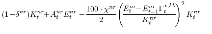
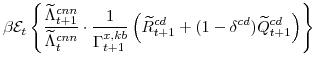
The symmetric first-order conditions implied by the non-residential part of the capital owners' profit-maximization problem (equation 17) are:
![\displaystyle Q^{nr}_{t} \left[A^{nr}_{t}-100\cdot\chi^{nr}\!\! \left(\frac{E^{nr}_{t}\!-\! E^{nr}_{t-1}\Gamma^{x,kb}_{t} } {K^{nr}_{t}}\right) \right]](img261.gif)
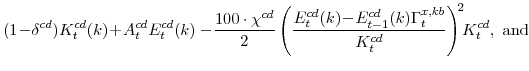
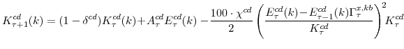
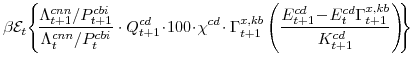
The symmetric first-order conditions implied by the consumer durables part of the capital owners' profit-maximization problem (equation 18) are:
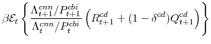
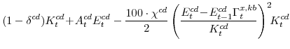
![\displaystyle Q^{cd}_{t} \left[A^{cd}_{t}-100\cdot\chi^{cd} \left(\frac{E^{cd}_{t}\!-\! E^{cd}_{t-1}\Gamma^{x,kb}_{t}} {K^{cd}_{t}}\right) \right]](img269.gif)
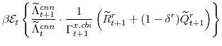
The symmetric first-order conditions implied by the residential part of the capital owners' profit-maximization problem (equation 19) are:

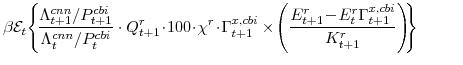
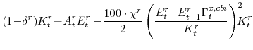
![\displaystyle Q^{r}_{t} \left[A^{r}_{t}-100\cdot\chi^{r} \left(\frac{E^{r}_{t}\!-\! E^{r}_{t-1}\Gamma^{x,cbi}_{t}} {K^{r}_{t}}\right) \right]](img276.gif)
The symmetric (expenditure-related) first-order conditions implied by the households' utility-maximization problem are: (equation 20) are:
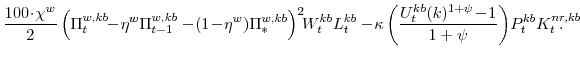
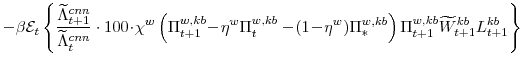
The key equations from the households' labor-supply decision are the wage Phillips curves

where
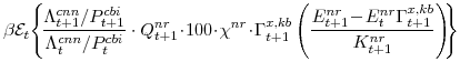
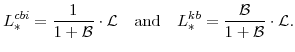
B. Equilibrium in the Symmetric and Stationary Model
The symmetric equilibrium is an allocation:
and a sequence of values
that satisfy the stationary versions of the equations given in the preceding section, taking as given the initial values of
The symmetric and stationary first-order conditions implied by the second step of the intermediate-goods producing firms' cost minimization problems (equation 15) are:

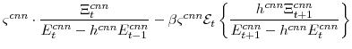
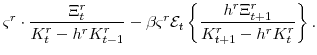
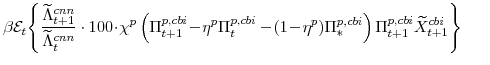
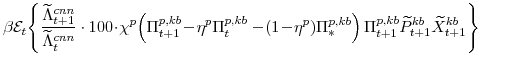
The stationary price Phillips curves that are implied by the intermediate-goods producing firms' profit maximization problems (equation 16) are
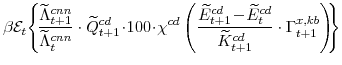
The symmetric and stationary first-order conditions implied by the non-residential part of the capital owners' profit-maximization problem (equation 17) are:

![\displaystyle \widetilde{Q}^{nr}_{t} \left[A^{nr}_{t}-100\cdot\chi^{nr}\!\! \left(\frac{\widetilde{E}^{nr}_{t}\!-\! \widetilde{E}^{nr}_{t-1}} {\widetilde{K}^{nr}_{t}}\cdot \Gamma^{x,kb}_{t}\right) \right]](img325.gif)
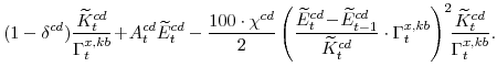
The symmetric and stationary first-order conditions implied by the consumer durables part of the capital owners'profit-maximization problem (equation 18) are:
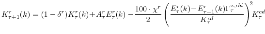
![\displaystyle \widetilde{Q}^{cd}_{t} \left[A^{cd}_{t}-100\cdot\chi^{cd} \left(\frac{\widetilde{E}^{cd}_{t}\!-\! \widetilde{E}^{cd}_{t-1}}{\widetilde{K}^{cd}_{t}}\cdot \Gamma^{x,kb}_{t}\right) \right]](img333.gif)
The symmetric and stationary first-order conditions implied by the residential part of the capital owners' profit-maximization problem (equation 19) are:
![\displaystyle \widetilde{Q}^{r}_{t} \left[A^{r}_{t}-100\cdot\chi^{r} \left(\frac{\widetilde{E}^{r}_{t}\!-\! \widetilde{E}^{r}_{t-1}}{\widetilde{K}^{r}_{t}}\cdot \Gamma^{x,cbi}_{t}\right) \right]](img340.gif)
The symmetric and stationary (expenditure-related) first-order conditions implied by the households' utility-maximization problem are: (equation 20) are:


The key equations from the households' labor-supply decision are the wage Phillips curves

The model's other conditions for equilibrium, listed in appendix A for the non-stationary model, are transformed as follows in the stationary model:
- The model's market clearing conditions become:

- The identities between real wages, relative prices, and wage and price inflation rates become:

- Equations (30) and (31) that describe the behavior of monetary policy are already described in terms of stationary variables;
- The equations that define the growth rates of GDP growth and price inflation are given by:
and
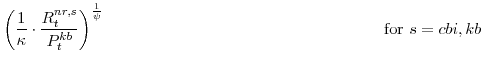
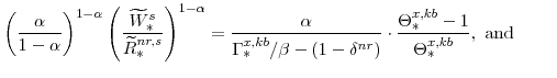
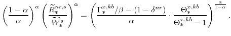
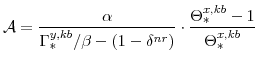
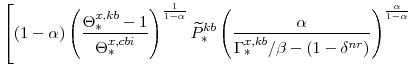
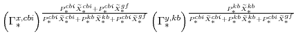
C. The Steady-state Solution to the Symmetric and Stationary Model
The steady-state growth rates in the fast- and slow-growing sectors of the economy are, respectively,
| (87) | |||
| (88) |
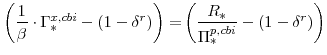
From the steady-state version of the Euler equation (equation 78), we know that the steady-state nominal interest rate is given by:
 |
(89) |
while the real interest rates relevant to consumers, capital owners, and producers respectively are:
 |
(90) | ||
 |
(91) |
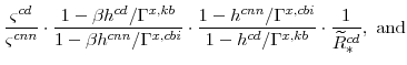
The steady-state values of the relative prices of fast-growing goods (
From our calibration of
 |
 |
||
 |
 |
From equations (72) and (75) note also that:
The steady-state inflation rates of capital prices and of nominal wages are given by:
| (97) | |||
| (98) |
where the steady-state inflation rate of consumption prices
The steady-state ratios
![]() ,
,
![]() ,
,
![]() , and
, and
![]() , which are calculated from the factor demand schedules (equations 61 and 62), are
, which are calculated from the factor demand schedules (equations 61 and 62), are

We can write these as

where
To solve for
![]() ,
,
![]() ,
,
![]() , and
, and
![]() by themselves we need to solve first for
by themselves we need to solve first for
![]() and
and
![]() . This takes a few steps, the first of which is to derive the ratio of
. This takes a few steps, the first of which is to derive the ratio of
![]() . As part of this excerise we must turn to considering the expenditure side of the model, and in particular the model's expenditure
ratios.
. As part of this excerise we must turn to considering the expenditure side of the model, and in particular the model's expenditure
ratios.
To calculate the model's expenditure ratios, we start with what we know about the ratios between the inputs to the optimizing household's utility function, that is
![]() ,
,
![]() , and
, and
![]() . We know from equations (79) to (83) that
. We know from equations (79) to (83) that
 |
|||
 |
We have expressions for
These equations imply that the ratios of expenditures implied by the optimizing agents of the model are

We can now consider expenditures as shares of their sector's outputs. Recall from the equilibrium conditions listed in appendix A that
|
This then allows us to write:
where
 |
We have expressions for
|
which can be re-arranged to
This then allows us to write:
so that
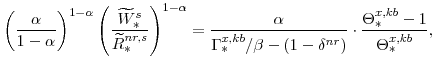
We now consider the household's supply of labor. First note from equations (60) and (81) that:
 |
Combining these steady-state values with the model's labor supply schedules (equations 84 and 85) and the expression for the steady-state real wage (equation 95), imply:
 |
|||
 |
|||
|
|||
 |
|||
|
|||
|
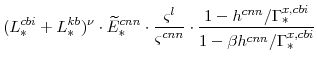
Letting
![\displaystyle \times \left.\frac{1+\mathcal{B}}{(\mathcal{A})^{\alpha/(1-\alpha)}}\cdot (1+\mathcal{R}) \cdot \frac{\varsigma^{cnn}}{\varsigma^{l}} \cdot \frac{1-\beta h^{cnn}/\Gamma^{x,cbi}}{1-h^{cnn}/\Gamma^{x,kb}} \right]^{\frac{1}{\nu+1}}](img467.gif)
Since the right-hand sides of equations (101) and (103) are identical,
-
 and
and
 (defined in equation 101) imply
 ;
; -
 and
and
 (defined in equation 103) imply
 ;
; -
and
 (defined in equation 100) imply
 and (since
 )
)
 ;
; -
and
 (defined in equation 102) imply
 and (since
 )
)
 ;
; -
,
, and the non-residential capital market clearing condition imply
 ;
; -
and
 and
and
 (both defined in equation 108) imply
 and
and
 ;
; -
and
 and
and
 (defined in equations 110 and 111) imply
 and
and
 ;
; -
and
, and
 and
and
 (both defined in equation 105) imply
 and
and
 ; and,
 -
 ,
,
 , and
, and
 are then implied by the steady-state versions of equations (81) to (83), while
 and
and
 are implied by the steady-state versions of equation (60).
|
|||
 |
The reader can verify that we have in this section presented a steady-state value for all of the model variables that defined equilibrium in appendix B.
D. List of Model Parameters
![]() Habit-persistence parameter for the consumption of non-durable goods and non-housing services.
Habit-persistence parameter for the consumption of non-durable goods and non-housing services.
![]() Habit-persistence parameter for the consumption of durable goods.
Habit-persistence parameter for the consumption of durable goods.
![]() Habit-persistence parameter for the consumption of housing services.
Habit-persistence parameter for the consumption of housing services.
![]() The elasticity of output with respect to capital.
The elasticity of output with respect to capital.
![]() The household's discount factor.
The household's discount factor.
![]() The quarterly depreciation rate of consumer durables.
The quarterly depreciation rate of consumer durables.
![]() The quarterly depreciation rate of non-residential capital.
The quarterly depreciation rate of non-residential capital.
![]() The quarterly depreciation rate of residential capital.
The quarterly depreciation rate of residential capital.
![]() Parameter reflecting the relative importance of lagged investment spending in the consumer durables adjustment cost function.
Parameter reflecting the relative importance of lagged investment spending in the consumer durables adjustment cost function.
![]() Parameter reflecting the relative importance of lagged investment spending in the non-residential capital adjustment cost function.
Parameter reflecting the relative importance of lagged investment spending in the non-residential capital adjustment cost function.
![]() Parameter reflecting the relative importance of lagged investment spending in the residential capital adjustment cost function.
Parameter reflecting the relative importance of lagged investment spending in the residential capital adjustment cost function.
![]() Parameter reflecting the relative importance of the lagged sectoral mix of non-residential capital in the non-residential capital sectoral adjustment cost function.
Parameter reflecting the relative importance of the lagged sectoral mix of non-residential capital in the non-residential capital sectoral adjustment cost function.
![]() Parameter reflecting the relative importance of the lagged sectoral mix of labor in the labor sectoral adjustment cost function.
Parameter reflecting the relative importance of the lagged sectoral mix of labor in the labor sectoral adjustment cost function.
![]() Parameter reflecting the relative importance of lagged price inflation in the adjustment cost function for prices.
Parameter reflecting the relative importance of lagged price inflation in the adjustment cost function for prices.
![]() Parameter reflecting the relative importance of lagged wage inflation in the adjustment cost function for wages.
Parameter reflecting the relative importance of lagged wage inflation in the adjustment cost function for wages.
![]() Variable capacity utilization scaling parameter.
Variable capacity utilization scaling parameter.
![]() Inverse labor supply elasticity.
Inverse labor supply elasticity.
![]() Persistence parameter in the AR(1) process describing the evolution of
Persistence parameter in the AR(1) process describing the evolution of
![]() .
.
![]() Persistence parameter in the AR(1) process describing the evolution of
Persistence parameter in the AR(1) process describing the evolution of
![]() .
.
![]() Persistence parameter in the AR(1) process describing the evolution of
Persistence parameter in the AR(1) process describing the evolution of ![]() .
.
![]() Persistence parameter in the AR(1) process describing the evolution of
Persistence parameter in the AR(1) process describing the evolution of
![]() .
.
![]() Persistence parameter in the AR(1) process describing the evolution of
Persistence parameter in the AR(1) process describing the evolution of
![]() .
.
![]() Persistence parameter in the AR(1) process describing the evolution of
Persistence parameter in the AR(1) process describing the evolution of
![]() .
.
![]() Persistence parameter in the AR(1) process describing the evolution of
Persistence parameter in the AR(1) process describing the evolution of
![]() .
.
![]() Persistence parameter in the AR(1) process describing the evolution of
Persistence parameter in the AR(1) process describing the evolution of
![]() .
.
![]() Persistence parameter in the AR(1) process describing the evolution of
Persistence parameter in the AR(1) process describing the evolution of
![]() .
.
![]() Persistence parameter in the AR(1) process describing the evolution of
Persistence parameter in the AR(1) process describing the evolution of
![]() .
.
![]() Persistence parameter in the AR(1) process describing the evolution of
Persistence parameter in the AR(1) process describing the evolution of
![]() .
.
![]() Persistence parameter in the AR(1) process describing the evolution of
Persistence parameter in the AR(1) process describing the evolution of
![]() .
.
![]() Co-efficient on the consumer non-durable goods and non-housing serives component of the utility function.
Co-efficient on the consumer non-durable goods and non-housing serives component of the utility function.
![]() Co-efficient on the consumer durable goods component of the utility function.
Co-efficient on the consumer durable goods component of the utility function.
![]() Co-efficient on the consumer housing serives component of the utility function.
Co-efficient on the consumer housing serives component of the utility function.
![]() Co-efficient on the labor supply components of the utility function.
Co-efficient on the labor supply components of the utility function.
![]() Co-efficient on GDP growth in the monetary policy reaction function.
Co-efficient on GDP growth in the monetary policy reaction function.
![]() Co-efficient on change in GDP growth in the monetary policy reaction function.
Co-efficient on change in GDP growth in the monetary policy reaction function.
![]() Co-efficient on GDP price inflation in the monetary policy reaction function.
Co-efficient on GDP price inflation in the monetary policy reaction function.
![]() Co-efficient on the change in GDP price inflation in the monetary policy reaction function.
Co-efficient on the change in GDP price inflation in the monetary policy reaction function.
![]() Co-efficient on lagged nominal interest rates in the monetary policy reaction function.
Co-efficient on lagged nominal interest rates in the monetary policy reaction function.
![]() Investment adjustment costs in the consumer durables evolution equation.
Investment adjustment costs in the consumer durables evolution equation.
![]() Investment adjustment costs in the non-residential capital evolution equation.
Investment adjustment costs in the non-residential capital evolution equation.
![]() Investment adjustment costs in the residential capital evolution equation.
Investment adjustment costs in the residential capital evolution equation.
![]() Parameter reflecting the size of adjustment costs in the labor sectoral adjustment cost function.
Parameter reflecting the size of adjustment costs in the labor sectoral adjustment cost function.
![]() Parameter reflecting the size of adjustment costs in re-setting prices.
Parameter reflecting the size of adjustment costs in re-setting prices.
![]() Parameter reflecting the size of adjustment costs in re-setting wages.
Parameter reflecting the size of adjustment costs in re-setting wages.
![]() Elasticity of utilization costs.
Elasticity of utilization costs.
E. List of Endogenous and Exogenous Model Variables
![]() Non-residential investment efficiency shock.
Non-residential investment efficiency shock.
![]() Residential investment efficiency shock.
Residential investment efficiency shock.
![]() Consumer durables investment efficiency shock.
Consumer durables investment efficiency shock.
![]() Expenditures on goods in the fast-growing "capital" goods sector for use in non-residential investment.
Expenditures on goods in the fast-growing "capital" goods sector for use in non-residential investment.
![]() Expenditures on goods in the slow-growing "consumption" goods sector for use in residential investment.
Expenditures on goods in the slow-growing "consumption" goods sector for use in residential investment.
![]() Expenditures on goods in the fast-growing "capital" goods sector for use in consumer durables investment.
Expenditures on goods in the fast-growing "capital" goods sector for use in consumer durables investment.
![]() Expenditures on goods in the fast-growing "capital" goods sector for use in consumer non-durable goods and non-housing services.
Expenditures on goods in the fast-growing "capital" goods sector for use in consumer non-durable goods and non-housing services.
![]() Exogenous expendiutre (by the government and foreign sector).
Exogenous expendiutre (by the government and foreign sector).
![]() Growth rate of real (chain-weighted) GDP.
Growth rate of real (chain-weighted) GDP.
![]() The amount of utilized non-residential capital used in the slow-growing "consumption"goods sector.
The amount of utilized non-residential capital used in the slow-growing "consumption"goods sector.
![]() The amount of utilized non-residential capital used in the fast-growing "capital" goods sector.
The amount of utilized non-residential capital used in the fast-growing "capital" goods sector.
![]() The physical amount of non-residential capital used in the slow-growing "consumption" goods sector.
The physical amount of non-residential capital used in the slow-growing "consumption" goods sector.
![]() The physical amount of non-residential capital used in the fast-growing "capital" goods sector.
The physical amount of non-residential capital used in the fast-growing "capital" goods sector.
![]() The aggregate non-residential capital stock.
The aggregate non-residential capital stock.
![]() The residential capital stock.
The residential capital stock.
![]() The consumer durables capital stock.
The consumer durables capital stock.
![]() Labor used in the slow-growing "consumption" goods sector.
Labor used in the slow-growing "consumption" goods sector.
![]() Labor used in the fast-growing "capital" goods sector.
Labor used in the fast-growing "capital" goods sector.
![]() Marginal cost in the slow-growing "consumption" goods sector.
Marginal cost in the slow-growing "consumption" goods sector.
![]() Marginal cost in the fast-growing "capital" goods sector.
Marginal cost in the fast-growing "capital" goods sector.
![]() Price level in the slow-growing "consumption" goods sector.
Price level in the slow-growing "consumption" goods sector.
![]() Price level in the fast-growing "capital" goods sector.
Price level in the fast-growing "capital" goods sector.
![]() Price of installed non-residential capital.
Price of installed non-residential capital.
![]() Price of installed residential capital.
Price of installed residential capital.
![]() Price of installed consumer durables capital.
Price of installed consumer durables capital.
![]() Nominal interest rate.
Nominal interest rate.
![]() The nominal rental rate on non-residential capital used in the slow-growing "consumption" goods sector.
The nominal rental rate on non-residential capital used in the slow-growing "consumption" goods sector.
![]() The nominal rental rate on non-residential capital used in the fast-growing "capital" goods sector.
The nominal rental rate on non-residential capital used in the fast-growing "capital" goods sector.
![]() The aggregate nominal rental rate on non-residential capital.
The aggregate nominal rental rate on non-residential capital.
![]() The nominal rental rate on residential capital.
The nominal rental rate on residential capital.
![]() The nominal rental rate on consumer durables capital.
The nominal rental rate on consumer durables capital.
![]() The utilization rate of non-residential capital used in the slow-growing "consumption" goods sector.
The utilization rate of non-residential capital used in the slow-growing "consumption" goods sector.
![]() The utilization rate of non-residential capital used in the fast-growing "capital" goods sector.
The utilization rate of non-residential capital used in the fast-growing "capital" goods sector.
![]() The nominal wage in the slow-growing "consumption" goods sector.
The nominal wage in the slow-growing "consumption" goods sector.
![]() The nominal wage in the fast-growing "capital" goods sector.
The nominal wage in the fast-growing "capital" goods sector.
![]() Production in the slow-growing "consumption" goods sector.
Production in the slow-growing "consumption" goods sector.
![]() Production in the fast-growing "capital" goods sector.
Production in the fast-growing "capital" goods sector.
![]() Level of capital-specific MFP.
Level of capital-specific MFP.
![]() Level of economy-wide MFP.
Level of economy-wide MFP.
![]() Growth rate of output in the consumption (slow growth) sector consistent with the growth rate of technology. (Note
Growth rate of output in the consumption (slow growth) sector consistent with the growth rate of technology. (Note
![]() is not in general equal to
is not in general equal to
![]() . Rather it is equal to
. Rather it is equal to
![]() .)
.)
![]() The growth rate of the level of capital-specific MFP.
The growth rate of the level of capital-specific MFP.
![]() The growth rate of the level of economy-wide MFP.
The growth rate of the level of economy-wide MFP.
![]() The elasticity of subsitution between the differentiated labor inputs into production.
The elasticity of subsitution between the differentiated labor inputs into production.
![]() The elasticity of subsitution between the differentiated intermediate inputs in the slow-growing "consumption" goods sector.
The elasticity of subsitution between the differentiated intermediate inputs in the slow-growing "consumption" goods sector.
![]() The elasticity of subsitution between the differentiated intermediate inputs in the fast-growing "capital" goods sector.
The elasticity of subsitution between the differentiated intermediate inputs in the fast-growing "capital" goods sector.
![]() The marginal utility of residential capital.
The marginal utility of residential capital.
![]() The marginal utility of durable goods.
The marginal utility of durable goods.
![]() The marginal utility of non-durable goods and non-housing services consumption.
The marginal utility of non-durable goods and non-housing services consumption.
![]() The marginal dis-utility of supplying labor in the slow-growing "consumption" goods sector.
The marginal dis-utility of supplying labor in the slow-growing "consumption" goods sector.
![]() The marginal dis-utility of supplying labor in the fast-growing "capital" goods sector.
The marginal dis-utility of supplying labor in the fast-growing "capital" goods sector.
![]() Consumer non-durable goods and non-housing services consumption preference shock.
Consumer non-durable goods and non-housing services consumption preference shock.
![]() Consumer durable capital stock preference shock.
Consumer durable capital stock preference shock.
![]() Residential capital stock preference shock.
Residential capital stock preference shock.
![]() Labor supply preference shock.
Labor supply preference shock.
![]() The inflation rate of the GDP deflator.
The inflation rate of the GDP deflator.
![]() The inflation rate for prices in the slow-growing "consumption" goods sector.
The inflation rate for prices in the slow-growing "consumption" goods sector.
![]() The inflation rate for prices in the fast-growing "capital" goods sector.
The inflation rate for prices in the fast-growing "capital" goods sector.
![]() The inflation rate of nominal wages in the slow-growing "consumption" goods sector.
The inflation rate of nominal wages in the slow-growing "consumption" goods sector.
![]() The inflation rate of nominal wages in the fast-growing "capital" goods sector.
The inflation rate of nominal wages in the fast-growing "capital" goods sector.
F. Definitions of Stationary Model Variables
In this section we provide definitions for all of the variables of the model that must be transformed in order to render them stationary. Note that in going through our list of model variables we leave out those that are already stationary.
The model's output variables in stationary form are:
 |
|||
 |
The model's expenditure variables in stationary form are:
 |
|||
 |
|||
 |
|||
 |
The model's marginal utility variables in stationary form are:
The model's capital stock variables in stationary form are:
 |
|||
 |
|||
 |
|||
 |
|||
 |
|||
 |
|||
 |
The model's relative (KB) output price variable in stationary form is:
 |
|||
 |
The model's real rental rate variables in stationary form are:
 |
|||
 |
|||
 |
|||
 |
|||
 |
The model's real marginal cost variables in stationary form are:
 |
|||
 |
The model's relative price of installed capital variables in stationary form are:
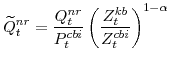 |
|||
 |
|||
 |
| Average Real Growth Rate |
Average Nominal Growth Rate |
Average Price Change* |
|
|---|---|---|---|
| Consumer non-durable goods and non-housing services | 3 1/4 percent | 6 1/4 percent | n.a. |
| Consumer housing services | 2 1/2 percent | 6 1/4 percent | 3/4 percent |
| Consumer durable goods | 6 3/4 percent | 6 1/2 percent | -3 percent |
| Res. investment goods | 3 3/4 percent | 7 1/2 percent | 1/2 percent |
| Non-res. investment goods | 6 1/4 percent | 6 1/4 percent | -2 3/4 percent |
*Relative to cons. non-durable goods & non-housing services prices.
| -4 | -3 | -2 | -1 | 0 | +1 | +2 | +3 | +4 | |
|---|---|---|---|---|---|---|---|---|---|
| Cons. non-dur. goods & non-hous. services | -0.03 | 0.08 | 0.23 | 0.28 | 0.43 | 0.37 | 0.28 | 0.28 | 0.18 |
| Cons. dur. goods | 0.10 | 0.06 | 0.14 | 0.25 | 0.32 | 0.06 | 0.06 | 0.08 | 0.07 |
| Res. inv. goods | 0.15 | 0.19 | 0.34 | 0.31 | 0.44 | 0.15 | - 0.08 | - 0.12 | - 0.15 |
| Non-res. inv. goods | 0.12 | 0.01 | 0.17 | 0.14 | 0.61 | 0.31 | 0.26 | -0.09 | -0.02 |
| Param. | Prior Type |
Prior Mean |
Prior S.D. |
Posterior Mode |
Posterior S.D. |
Posterior 10th perc. |
Posterior 50th perc. |
Posterior 90th perc. |
|---|---|---|---|---|---|---|---|---|
| B | 0.500 | 0.122 | 0.766 | 0.048 | 0.707 | 0.770 | 0.828 | |
| B | 0.500 | 0.122 | 0.571 | 0.196 | 0.372 | 0.600 | 0.919 | |
| B | 0.500 | 0.122 | 0.500 | 0.128 | 0.328 | 0.490 | 0.665 | |
| G | 2.000 | 1.000 | 1.287 | 0.735 | 0.805 | 1.554 | 2.600 | |
| G | 2.000 | 1.000 | 2.331 | 0.808 | 2.294 | 3.193 | 4.338 | |
| B | 0.500 | 0.224 | 0.257 | 0.124 | 0.163 | 0.313 | 0.481 | |
| G | 2.000 | 1.000 | 1.555 | 1.478 | 1.268 | 2.750 | 4.944 | |
| B | 0.500 | 0.224 | 0.296 | 0.147 | 0.138 | 0.328 | 0.529 | |
| G | 2.000 | 1.000 | 0.831 | 0.397 | 0.676 | 1.053 | 1.665 | |
| G | 2.000 | 1.000 | 0.145 | 0.082 | 0.055 | 0.181 | 0.275 | |
| G | 6.000 | 1.000 | 10.198 | 2.590 | 8.085 | 10.852 | 14.793 | |
| G | 2.000 | 1.000 | 0.766 | 1.703 | 0.412 | 1.366 | 3.615 | |
| B | 0.500 | 0.224 | 0.779 | 0.202 | 0.377 | 0.702 | 0.910 | |
| N | 2.000 | 1.000 | 3.532 | 0.515 | 2.947 | 3.561 | 4.251 | |
|
|
N | 0.500 | 0.400 | -0.041 | 0.080 | -0.137 | -0.040 | 0.070 |
| N | 0.500 | 0.400 | 0.210 | 0.026 | 0.183 | 0.216 | 0.250 | |
|
|
N | 0.500 | 0.400 | -0.084 | 0.025 | -0.124 | -0.092 | -0.059 |
| B | 0.750 | 0.112 | 0.900 | 0.018 | 0.876 | 0.902 | 0.922 |
| Param. | Prior Type |
Prior Mean |
Prior S.D. |
Posterior Mode |
Posterior S.D. |
Posterior 10th perc. |
Posterior 50th perc. |
Posterior 90th perc. |
|---|---|---|---|---|---|---|---|---|
|
|
B | 0.750 | 0.112 | 0.894 | 0.032 | 0.839 | 0.884 | 0.920 |
|
|
B | 0.750 | 0.112 | 0.842 | 0.115 | 0.619 | 0.802 | 0.908 |
|
|
B | 0.500 | 0.150 | 0.527 | 0.103 | 0.379 | 0.519 | 0.648 |
|
|
B | 0.750 | 0.112 | 0.795 | 0.079 | 0.660 | 0.778 | 0.867 |
|
|
B | 0.750 | 0.112 | 0.899 | 0.080 | 0.733 | 0.859 | 0.931 |
|
|
B | 0.750 | 0.112 | 0.793 | 0.113 | 0.615 | 0.787 | 0.907 |
|
|
B | 0.750 | 0.112 | 0.940 | 0.030 | 0.884 | 0.930 | 0.962 |
|
|
B | 0.500 | 0.150 | 0.305 | 0.079 | 0.211 | 0.315 | 0.418 |
|
|
B | 0.750 | 0.112 | 0.927 | 0.051 | 0.823 | 0.903 | 0.949 |
|
|
B | 0.750 | 0.112 | 0.982 | 0.014 | 0.957 | 0.978 | 0.990 |
|
|
I | 4.000 | 2.000 | 6.631 | 2.056 | 5.986 | 8.032 | 11.069 |
|
|
I | 2.000 | 2.000 | 1.795 | 0.839 | 1.385 | 2.367 | 3.465 |
|
|
I | 4.000 | 2.000 | 8.168 | 2.505 | 6.181 | 8.724 | 12.737 |
|
|
I | 3.000 | 2.000 | 1.555 | 0.319 | 1.344 | 1.634 | 2.089 |
|
|
I | 3.000 | 2.000 | 3.304 | 1.995 | 2.192 | 3.670 | 6.967 |
|
|
I | 3.000 | 2.000 | 2.453 | 4.550 | 2.094 | 3.976 | 11.102 |
|
|
I | 3.000 | 2.000 | 2.175 | 0.877 | 2.049 | 2.973 | 4.273 |
|
|
I | 0.200 | 2.000 | 0.112 | 0.011 | 0.101 | 0.114 | 0.130 |
|
|
I | 0.500 | 2.000 | 0.766 | 0.067 | 0.688 | 0.769 | 0.859 |
|
|
I | 0.500 | 2.000 | 0.294 | 0.105 | 0.269 | 0.357 | 0.529 |
|
|
I | 1.000 | 2.000 | 1.507 | 0.154 | 1.363 | 1.533 | 1.744 |
|
|
I | 0.500 | 2.000 | 0.526 | 0.200 | 0.496 | 0.703 | 0.995 |
|
|
I | 0.500 | 2.000 | 0.394 | 0.164 | 0.326 | 0.485 | 0.752 |
|
|
I | 0.500 | 2.000 | 0.667 | 0.088 | 0.563 | 0.667 | 0.786 |
| Shocks |
|
||
|---|---|---|---|
|
|
(0.02,0.02,0.03) | (0.00,0.00,0.01) | (0.01,0.02,0.02) |
|
|
(0.01,0.01,0.01) | (0.01,0.01,0.02) | (0.04,0.05,0.06) |
|
|
(0.00,0.00,0.00) | (0.01,0.01,0.02) | (0.03,0.04,0.05) |
|
|
(0.00,0.00,0.00) | (0.01,0.01,0.01) | (0.03,0.05,0.06) |
|
|
(0.01,0.03,0.04) | (0.00,0.00,0.01) | (0.01,0.02,0.03) |
|
|
(0.00,0.01,0.01) | (0.00,0.01,0.02) | (0.02,0.04,0.07) |
|
|
(0.00,0.00,0.00) | (0.00,0.01,0.02) | (0.01,0.03,0.06) |
|
|
(0.00,0.00,0.00) | (0.00,0.00,0.01) | (0.01,0.02,0.03) |
|
|
(0.00,0.00,0.00) | (0.00,0.00,0.00) | (0.00,0.00,0.00) |
|
|
(0.00,0.00,0.00) | (0.00,0.00,0.00) | (0.00,0.00,0.00) |
|
|
(0.00,0.00,0.00) | (0.00,0.00,0.00) | (0.00,0.00,0.00) |
|
|
(0.00,0.00,0.00) | (0.00,0.00,0.00) | (0.00,0.00,0.00) |
|
|
(0.01,0.01,0.01) | (0.03,0.04,0.05) | (0.00,0.00,0.00) |
|
|
(0.03,0.04,0.05) | (0.08,0.10,0.14) | (0.00,0.00,0.01) |
|
|
(0.04,0.05,0.07) | (0.07,0.09,0.12) | (0.00,0.00,0.00) |
|
|
(0.00,0.00,0.01) | (0.00,0.00,0.01) | (0.00,0.00,0.00) |
|
|
(0.02,0.03,0.04) | (0.02,0.02,0.03) | (0.50,0.57,0.63) |
|
|
(0.01,0.01,0.02) | (0.05,0.07,0.09) | (0.05,0.07,0.08) |
|
|
(0.00,0.00,0.00) | (0.06,0.08,0.10) | (0.01,0.01,0.02) |
|
|
(0.00,0.00,0.00) | (0.04,0.06,0.08) | (0.01,0.01,0.01) |
|
|
(0.00,0.00,0.00) | (0.03,0.04,0.06) | (0.01,0.01,0.02) |
|
|
(0.01,0.02,0.03) | (0.12,0.15,0.19) | (0.02,0.04,0.06) |
|
|
(0.07,0.09,0.12) | (0.19,0.24,0.29) | (0.02,0.04,0.06) |
|
|
(0.49,0.59,0.69) | (0.43,0.54,0.65) | (0.00,0.01,0.02) |
|
|
(0.32,0.36,0.40) | (0.18,0.22,0.27) | (0.01,0.03,0.05) |
|
|
(0.29,0.35,0.41) | (0.44,0.50,0.56) | (0.01,0.02,0.03) |
|
|
(0.31,0.38,0.44) | (0.40,0.46,0.53) | (0.00,0.01,0.01) |
|
|
(0.28,0.37,0.47) | (0.20,0.27,0.35) | (0.02,0.03,0.05) |
| Shocks |
|
||
|---|---|---|---|
|
|
(0.00,0.01,0.01) | (0.51,0.58,0.66) | (0.07,0.10,0.13) |
|
|
(0.00,0.00,0.00) | (0.02,0.03,0.04) | (0.02,0.03,0.05) |
|
|
(0.00,0.00,0.00) | (0.00,0.00,0.01) | (0.01,0.01,0.02) |
|
|
(0.00,0.00,0.00) | (0.00,0.00,0.00) | (0.00,0.01,0.01) |
|
|
(0.00,0.00,0.00) | (0.01,0.02,0.03) | (0.00,0.00,0.00) |
|
|
(0.00,0.00,0.00) | (0.00,0.00,0.00) | (0.00,0.00,0.00) |
|
|
(0.00,0.00,0.00) | (0.00,0.00,0.00) | (0.00,0.00,0.00) |
|
|
(0.00,0.00,0.00) | (0.00,0.00,0.00) | (0.00,0.00,0.00) |
|
|
(0.00,0.00,0.00) | (0.02,0.03,0.04) | (0.00,0.00,0.00) |
|
|
(0.00,0.01,0.01) | (0.02,0.03,0.04) | (0.00,0.00,0.01) |
|
|
(0.00,0.00,0.00) | (0.00,0.01,0.01) | (0.00,0.00,0.00) |
|
|
(0.00,0.00,0.00) | (0.00,0.00,0.00) | (0.00,0.00,0.00) |
|
|
(0.01,0.01,0.01) | (0.00,0.00,0.00) | (0.00,0.01,0.01) |
|
|
(0.00,0.00,0.00) | (0.00,0.00,0.00) | (0.01,0.01,0.01) |
|
|
(0.00,0.00,0.00) | (0.00,0.00,0.01) | (0.01,0.01,0.01) |
|
|
(0.00,0.00,0.00) | (0.00,0.00,0.01) | (0.01,0.01,0.02) |
|
|
(0.02,0.04,0.06) | (0.00,0.00,0.01) | (0.01,0.03,0.04) |
|
|
(0.00,0.01,0.02) | (0.00,0.01,0.02) | (0.03,0.07,0.11) |
|
|
(0.00,0.00,0.00) | (0.00,0.01,0.02) | (0.01,0.04,0.07) |
|
|
(0.00,0.00,0.00) | (0.00,0.00,0.01) | (0.00,0.01,0.03) |
|
|
(0.21,0.25,0.29) | (0.00,0.00,0.01) | (0.09,0.11,0.14) |
|
|
(0.43,0.50,0.56) | (0.00,0.01,0.03) | (0.54,0.59,0.65) |
|
|
(0.35,0.43,0.51) | (0.00,0.01,0.04) | (0.73,0.77,0.81) |
|
|
(0.00,0.01,0.02) | (0.04,0.07,0.10) | (0.75,0.80,0.84) |
|
|
(0.21,0.23,0.26) | (0.00,0.01,0.01) | (0.06,0.08,0.10) |
|
|
(0.03,0.03,0.04) | (0.01,0.02,0.03) | (0.03,0.03,0.04) |
|
|
(0.02,0.03,0.03) | (0.01,0.02,0.03) | (0.01,0.01,0.02) |
|
|
(0.00,0.01,0.01) | (0.00,0.00,0.00) | (0.01,0.02,0.03) |
| Shocks |
|
|
|
|
|---|---|---|---|---|
|
|
(0.15,0.18,0.20) | (0.01,0.01,0.02) | (0.01,0.01,0.02) | (0.00,0.00,0.00) |
|
|
(0.22,0.26,0.31) | (0.02,0.03,0.04) | (0.01,0.02,0.02) | (0.00,0.00,0.00) |
|
|
(0.20,0.25,0.31) | (0.03,0.04,0.08) | (0.01,0.02,0.03) | (0.00,0.00,0.00) |
|
|
(0.02,0.02,0.04) | (0.00,0.01,0.01) | (0.01,0.01,0.02) | (0.00,0.00,0.00) |
|
|
(0.00,0.00,0.00) | (0.00,0.00,0.01) | (0.13,0.26,0.44) | (0.00,0.00,0.00) |
|
|
(0.00,0.00,0.01) | (0.00,0.01,0.01) | (0.12,0.27,0.45) | (0.00,0.00,0.00) |
|
|
(0.00,0.00,0.01) | (0.00,0.01,0.02) | (0.11,0.31,0.49) | (0.00,0.00,0.00) |
|
|
(0.00,0.00,0.00) | (0.00,0.00,0.00) | (0.06,0.16,0.31) | (0.00,0.00,0.00) |
|
|
(0.00,0.00,0.00) | (0.00,0.00,0.02) | (0.00,0.00,0.00) | (0.00,0.00,0.00) |
|
|
(0.00,0.00,0.00) | (0.00,0.01,0.04) | (0.00,0.00,0.00) | (0.00,0.00,0.00) |
|
|
(0.00,0.00,0.00) | (0.00,0.01,0.06) | (0.00,0.00,0.00) | (0.00,0.00,0.00) |
|
|
(0.00,0.00,0.00) | (0.00,0.00,0.00) | (0.00,0.00,0.00) | (0.00,0.00,0.00) |
|
|
(0.00,0.00,0.01) | (0.01,0.01,0.01) | (0.00,0.00,0.00) | (0.00,0.00,0.00) |
|
|
(0.01,0.02,0.03) | (0.02,0.03,0.05) | (0.00,0.00,0.01) | (0.00,0.00,0.00) |
|
|
(0.03,0.05,0.07) | (0.07,0.10,0.13) | (0.01,0.02,0.02) | (0.00,0.01,0.01) |
|
|
(0.04,0.06,0.09) | (0.06,0.09,0.13) | (0.06,0.09,0.13) | (0.02,0.04,0.07) |
|
|
(0.00,0.00,0.01) | (0.00,0.01,0.01) | (0.02,0.02,0.03) | (0.00,0.00,0.01) |
|
|
(0.00,0.01,0.01) | (0.01,0.01,0.01) | (0.01,0.01,0.02) | (0.00,0.00,0.00) |
|
|
(0.00,0.01,0.01) | (0.01,0.01,0.02) | (0.01,0.01,0.01) | (0.00,0.00,0.00) |
|
|
(0.00,0.00,0.00) | (0.00,0.00,0.00) | (0.00,0.01,0.01) | (0.00,0.00,0.00) |
|
|
(0.00,0.00,0.01) | (0.00,0.01,0.01) | (0.02,0.04,0.05) | (0.01,0.02,0.03) |
|
|
(0.01,0.02,0.04) | (0.02,0.03,0.04) | (0.03,0.04,0.06) | (0.01,0.02,0.04) |
|
|
(0.05,0.08,0.13) | (0.07,0.09,0.13) | (0.04,0.05,0.07) | (0.01,0.02,0.04) |
|
|
(0.27,0.35,0.43) | (0.05,0.08,0.14) | (0.13,0.21,0.30) | (0.00,0.01,0.02) |
|
|
(0.73,0.76,0.80) | (0.00,0.00,0.00) | (0.01,0.02,0.03) | (0.00,0.00,0.00) |
|
|
(0.55,0.61,0.67) | (0.00,0.00,0.00) | (0.00,0.01,0.02) | (0.00,0.00,0.00) |
|
|
(0.47,0.55,0.62) | (0.01,0.02,0.03) | (0.00,0.00,0.01) | (0.00,0.00,0.00) |
|
|
(0.13,0.17,0.21) | (0.09,0.12,0.16) | (0.01,0.02,0.04) | (0.01,0.02,0.03) |
| Shocks |
|
|
|
|
|---|---|---|---|---|
|
|
(0.00,0.00,0.01) | (0.00,0.00,0.01) | (0.00,0.00,0.00) | (0.00,0.00,0.00) |
|
|
(0.00,0.01,0.01) | (0.00,0.01,0.01) | (0.00,0.00,0.00) | (0.00,0.00,0.00) |
|
|
(0.00,0.01,0.01) | (0.01,0.01,0.01) | (0.00,0.00,0.00) | (0.00,0.00,0.00) |
|
|
(0.00,0.00,0.00) | (0.00,0.00,0.00) | (0.00,0.00,0.00) | (0.00,0.00,0.00) |
|
|
(0.00,0.00,0.00) | (0.00,0.00,0.00) | (0.00,0.00,0.00) | (0.00,0.00,0.00) |
|
|
(0.00,0.00,0.00) | (0.00,0.00,0.00) | (0.00,0.00,0.00) | (0.00,0.00,0.00) |
|
|
(0.00,0.00,0.00) | (0.00,0.00,0.00) | (0.00,0.00,0.00) | (0.00,0.00,0.00) |
|
|
(0.00,0.00,0.00) | (0.00,0.00,0.00) | (0.00,0.00,0.00) | (0.00,0.00,0.00) |
|
|
(0.00,0.00,0.00) | (0.00,0.00,0.00) | (0.00,0.00,0.00) | (0.00,0.00,0.00) |
|
|
(0.00,0.00,0.00) | (0.00,0.00,0.01) | (0.00,0.00,0.00) | (0.00,0.00,0.00) |
|
|
(0.00,0.00,0.01) | (0.00,0.01,0.01) | (0.00,0.00,0.01) | (0.00,0.00,0.00) |
|
|
(0.00,0.00,0.00) | (0.00,0.00,0.00) | (0.00,0.00,0.01) | (0.00,0.00,0.00) |
|
|
(0.00,0.00,0.00) | (0.85,0.88,0.91) | (0.00,0.00,0.00) | (0.00,0.00,0.00) |
|
|
(0.00,0.00,0.00) | (0.68,0.76,0.83) | (0.00,0.00,0.00) | (0.00,0.00,0.00) |
|
|
(0.00,0.00,0.01) | (0.46,0.58,0.67) | (0.00,0.00,0.00) | (0.00,0.00,0.00) |
|
|
(0.00,0.00,0.00) | (0.00,0.00,0.01) | (0.00,0.00,0.00) | (0.00,0.00,0.00) |
|
|
(0.00,0.00,0.00) | (0.00,0.00,0.00) | (0.19,0.34,0.50) | (0.00,0.00,0.00) |
|
|
(0.00,0.00,0.00) | (0.00,0.00,0.00) | (0.10,0.23,0.40) | (0.00,0.00,0.00) |
|
|
(0.00,0.00,0.00) | (0.00,0.00,0.00) | (0.05,0.15,0.33) | (0.00,0.00,0.00) |
|
|
(0.00,0.00,0.00) | (0.00,0.00,0.00) | (0.01,0.02,0.06) | (0.00,0.00,0.00) |
|
|
(0.02,0.03,0.04) | (0.03,0.05,0.07) | (0.20,0.24,0.29) | (0.95,0.97,0.98) |
|
|
(0.02,0.04,0.06) | (0.02,0.05,0.10) | (0.27,0.33,0.40) | (0.95,0.97,0.98) |
|
|
(0.00,0.00,0.01) | (0.00,0.01,0.03) | (0.24,0.34,0.43) | (0.94,0.96,0.98) |
|
|
(0.25,0.34,0.43) | (0.54,0.64,0.71) | (0.24,0.34,0.46) | (0.87,0.92,0.95) |
|
|
(0.00,0.00,0.00) | (0.00,0.00,0.00) | (0.01,0.01,0.01) | (0.00,0.00,0.00) |
|
|
(0.00,0.00,0.00) | (0.00,0.00,0.01) | (0.00,0.01,0.01) | (0.00,0.00,0.00) |
|
|
(0.00,0.00,0.00) | (0.00,0.00,0.01) | (0.00,0.00,0.01) | (0.00,0.00,0.00) |
|
|
(0.00,0.00,0.00) | (0.00,0.00,0.00) | (0.00,0.00,0.00) | (0.00,0.00,0.00) |
| Shocks | ||||
|---|---|---|---|---|
|
|
(0.03,0.04,0.06) | (0.00,0.00,0.00) | (0.00,0.00,0.01) | (0.00,0.00,0.00) |
|
|
(0.03,0.04,0.05) | (0.00,0.01,0.01) | (0.01,0.01,0.02) | (0.00,0.00,0.00) |
|
|
(0.02,0.03,0.03) | (0.01,0.01,0.01) | (0.01,0.02,0.03) | (0.00,0.00,0.00) |
|
|
(0.01,0.02,0.03) | (0.01,0.01,0.02) | (0.01,0.02,0.03) | (0.00,0.00,0.00) |
|
|
(0.02,0.05,0.08) | (0.00,0.00,0.00) | (0.00,0.00,0.00) | (0.00,0.00,0.01) |
|
|
(0.02,0.04,0.06) | (0.00,0.01,0.01) | (0.00,0.01,0.02) | (0.00,0.00,0.01) |
|
|
(0.01,0.02,0.04) | (0.00,0.01,0.01) | (0.00,0.01,0.02) | (0.00,0.00,0.01) |
|
|
(0.00,0.01,0.01) | (0.00,0.00,0.01) | (0.00,0.01,0.01) | (0.00,0.00,0.00) |
|
|
(0.00,0.00,0.00) | (0.00,0.00,0.00) | (0.00,0.00,0.00) | (0.00,0.00,0.00) |
|
|
(0.00,0.00,0.00) | (0.00,0.00,0.00) | (0.00,0.00,0.00) | (0.00,0.00,0.00) |
|
|
(0.00,0.00,0.00) | (0.00,0.00,0.00) | (0.00,0.00,0.00) | (0.00,0.00,0.00) |
|
|
(0.00,0.00,0.00) | (0.00,0.00,0.00) | (0.00,0.00,0.00) | (0.00,0.00,0.00) |
|
|
(0.01,0.02,0.03) | (0.05,0.09,0.14) | (0.02,0.03,0.04) | (0.02,0.02,0.03) |
|
|
(0.05,0.07,0.10) | (0.31,0.41,0.52) | (0.09,0.12,0.15) | (0.03,0.03,0.05) |
|
|
(0.13,0.18,0.25) | (0.14,0.21,0.30) | (0.09,0.12,0.16) | (0.02,0.02,0.03) |
|
|
(0.47,0.60,0.71) | (0.00,0.00,0.00) | (0.00,0.01,0.01) | (0.00,0.00,0.00) |
|
|
(0.05,0.06,0.07) | (0.01,0.01,0.02) | (0.01,0.02,0.02) | (0.01,0.02,0.02) |
|
|
(0.04,0.05,0.07) | (0.08,0.10,0.13) | (0.06,0.08,0.10) | (0.02,0.03,0.04) |
|
|
(0.03,0.04,0.05) | (0.07,0.10,0.13) | (0.08,0.10,0.12) | (0.02,0.02,0.03) |
|
|
(0.01,0.01,0.02) | (0.05,0.07,0.12) | (0.08,0.11,0.13) | (0.01,0.01,0.01) |
|
|
(0.03,0.05,0.06) | (0.00,0.00,0.00) | (0.00,0.00,0.01) | (0.30,0.38,0.47) |
|
|
(0.04,0.05,0.07) | (0.00,0.01,0.02) | (0.01,0.02,0.03) | (0.62,0.69,0.74) |
|
|
(0.03,0.04,0.06) | (0.00,0.00,0.01) | (0.01,0.02,0.04) | (0.76,0.81,0.85) |
|
|
(0.00,0.00,0.01) | (0.09,0.16,0.25) | (0.05,0.11,0.20) | (0.91,0.94,0.96) |
|
|
(0.24,0.28,0.32) | (0.00,0.00,0.01) | (0.13,0.17,0.22) | (0.11,0.14,0.18) |
|
|
(0.09,0.12,0.16) | (0.00,0.00,0.02) | (0.51,0.57,0.63) | (0.13,0.17,0.22) |
|
|
(0.02,0.04,0.06) | (0.01,0.03,0.06) | (0.53,0.59,0.65) | (0.08,0.11,0.15) |
|
|
(0.00,0.00,0.01) | (0.16,0.22,0.29) | (0.43,0.51,0.59) | (0.03,0.04,0.06) |
| Shocks | ||||
|---|---|---|---|---|
|
|
(0.01,0.01,0.02) | (0.00,0.00,0.00) | (0.66,0.73,0.79) | (0.00,0.00,0.00) |
|
|
(0.01,0.01,0.01) | (0.00,0.00,0.00) | (0.04,0.06,0.08) | (0.00,0.00,0.00) |
|
|
(0.00,0.00,0.01) | (0.00,0.00,0.00) | (0.00,0.01,0.01) | (0.00,0.00,0.00) |
|
|
(0.00,0.00,0.00) | (0.00,0.00,0.00) | (0.00,0.00,0.00) | (0.00,0.00,0.00) |
|
|
(0.00,0.00,0.00) | (0.00,0.00,0.00) | (0.00,0.00,0.00) | (0.25,0.35,0.45) |
|
|
(0.00,0.00,0.00) | (0.00,0.00,0.00) | (0.00,0.00,0.00) | (0.01,0.01,0.01) |
|
|
(0.00,0.00,0.00) | (0.00,0.00,0.00) | (0.00,0.00,0.00) | (0.00,0.00,0.00) |
|
|
(0.00,0.00,0.00) | (0.00,0.00,0.00) | (0.00,0.00,0.00) | (0.00,0.00,0.00) |
|
|
(0.00,0.01,0.01) | (0.80,0.87,0.92) | (0.01,0.02,0.03) | (0.01,0.02,0.02) |
|
|
(0.01,0.02,0.02) | (0.07,0.12,0.21) | (0.02,0.03,0.04) | (0.01,0.01,0.01) |
|
|
(0.01,0.02,0.03) | (0.00,0.00,0.01) | (0.00,0.01,0.01) | (0.00,0.00,0.00) |
|
|
(0.01,0.01,0.02) | (0.00,0.00,0.00) | (0.00,0.00,0.00) | (0.00,0.00,0.00) |
|
|
(0.01,0.01,0.02) | (0.00,0.00,0.00) | (0.00,0.00,0.00) | (0.00,0.00,0.00) |
|
|
(0.01,0.01,0.01) | (0.00,0.00,0.00) | (0.00,0.00,0.01) | (0.00,0.00,0.00) |
|
|
(0.00,0.00,0.01) | (0.00,0.00,0.00) | (0.00,0.01,0.01) | (0.00,0.00,0.00) |
|
|
(0.00,0.00,0.00) | (0.00,0.00,0.01) | (0.00,0.01,0.01) | (0.00,0.00,0.00) |
|
|
(0.04,0.08,0.11) | (0.00,0.00,0.00) | (0.00,0.00,0.01) | (0.00,0.01,0.01) |
|
|
(0.03,0.06,0.09) | (0.01,0.01,0.03) | (0.00,0.01,0.03) | (0.00,0.00,0.01) |
|
|
(0.01,0.02,0.05) | (0.00,0.01,0.02) | (0.00,0.01,0.03) | (0.00,0.00,0.01) |
|
|
(0.00,0.00,0.01) | (0.00,0.00,0.01) | (0.00,0.00,0.01) | (0.00,0.00,0.00) |
|
|
(0.29,0.34,0.39) | (0.00,0.01,0.02) | (0.00,0.00,0.01) | (0.01,0.02,0.04) |
|
|
(0.41,0.47,0.53) | (0.12,0.20,0.32) | (0.00,0.01,0.04) | (0.00,0.01,0.03) |
|
|
(0.47,0.53,0.60) | (0.43,0.56,0.66) | (0.00,0.02,0.06) | (0.00,0.01,0.02) |
|
|
(0.21,0.31,0.42) | (0.34,0.46,0.58) | (0.10,0.15,0.22) | (0.00,0.00,0.01) |
|
|
(0.02,0.03,0.03) | (0.00,0.01,0.01) | (0.00,0.01,0.01) | (0.00,0.01,0.01) |
|
|
(0.02,0.02,0.03) | (0.02,0.03,0.05) | (0.01,0.02,0.03) | (0.00,0.01,0.01) |
|
|
(0.01,0.02,0.02) | (0.02,0.03,0.04) | (0.01,0.02,0.03) | (0.00,0.00,0.01) |
|
|
(0.00,0.00,0.01) | (0.00,0.00,0.01) | (0.00,0.00,0.01) | (0.00,0.00,0.00) |
Notes:
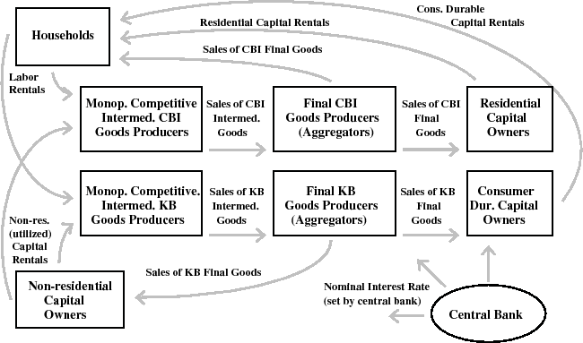
- CBI represents the economy's slow growing sector, so denoted because consumption [C] goods and services account for most of its output and it is produced by the business and institutions [BI] sector of the economy.
- KB represents the economy's fast growing sector, so denoted because its output is capital [K] goods and it is produced by the business [B] sector of the economy.