Skip to: [Printable Version (PDF)] [Bibliography] [Footnotes]

Finance and Economics Discussion Series: 2008-01 Screen Reader version ^♣

The Jumbo-Conforming Spread: A Semiparametric Approach ¹

Shane M. Sherlund Board of Governors of the Federal Reserve System Washington, DC 20551 (202) 452-3589 [email protected]

All comments are welcome.

Keywords: Mortgages, jumbo-conforming spread, partial-linear regression, local-linear regression.

Abstract:

This paper estimates the jumbo-conforming spread using data from the Federal Housing Finance Board's Monthly Interest Rate Survey from January 1993 to June 2007. Importantly, this paper augments the typical parametric approach by adding state-level foreclosure laws and ZIP-level demographic variables to the model, estimating the effects of loan size and loan-to-value ratio on mortgage rates nonparametrically, and including geographic location as a control for some potentially unobserved borrower and market characteristics that might vary over geography, such as credit scores, debt-to-income ratios, and house price volatility. A partial local-linear regression approach is used to estimate the jumbo-conforming spread, on the premise that loans similar to each other in terms of loan size, loan-to-value ratio, or geographic location might also be similar in other, unobservable borrower and market characteristics. I find estimates of the jumbo-conforming spread of 13 to 24 basis points--50 to 24 percent smaller since about 1996, when credit scores became widely used in mortgage underwriting, than estimates from a commonly used parametric model. I therefore attribute the difference in estimates to credit quality and other unobserved characteristics, among other potential explanations, making these controls an important issue in estimating the jumbo-conforming spread.

Journal of Economic Literature classification numbers: G21, G28.

1 Introduction

The housing government-sponsored enterprises (GSEs), Fannie Mae and Freddie Mac, were created by Congress to facilitate the flow of capital to lenders for making mortgage loans. The GSEs, as well as private-label issuers, purchase mortgages from lenders and package them together as mortgage-backed securities (MBS). The resulting securities can then be sold to investors. This process, known as securitization (or MBS issuance), frees lenders' capital, thereby making it possible for lenders to extend more mortgage loans.

The effect of GSE activities on mortgage rates, in particular, has prompted considerable previous work. Some research argues that the GSEs serve to reduce interest rates on so-called conforming mortgages--those that the housing GSEs are eligible to purchase--by facilitating securitization of these mortgages relative to so-called jumbo mortgages--those that exceed the conforming loan limit and which the GSEs are ineligible to purchase. Other research argues that the jumbo-conforming spread provides only an upper bound on the effect of the GSEs on mortgage rates.

As shown in Figure 1, average mortgage rates on jumbo originations have generally exceeded average mortgage rates on conforming originations over the 1993 to 2007 period. The figure also shows the dispersion of mortgage rates across loans at any given point in time, as shown by the range between the 10th and 90th percentiles for rates on conforming mortgages. The wide range of mortgage rates presumably reflects the effects of a variety of other factors on mortgage pricing, such as credit quality.

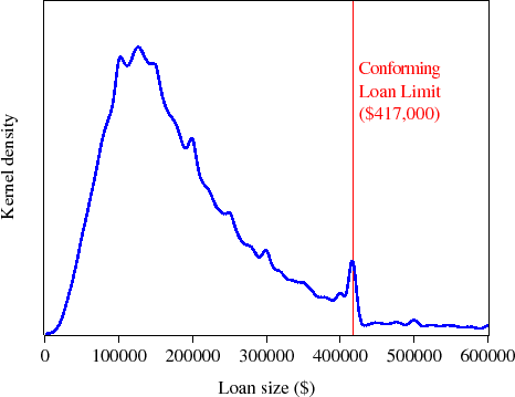
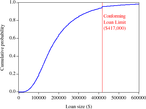
Figure 2 shows a kernel density estimate and Figure 3 shows the empirical cumulative distribution function for thirty-year fixed-rate mortgage loan sizes originated during 2006. Over 95 percent of these 30-year fixed-rate mortgage originations had loan sizes at or below the conforming loan limit, most with loan sizes between $100,000 and $200,000. In addition, the spike of loans at the conforming loan limit, and the relative dearth of loans just above the loan limit, suggest that at least some borrowers perceive a difference in rates on jumbo and conforming mortgages, and therefore select lower-cost conforming mortgages. Some observers have argued that these empirical facts suggest that GSE securitization activity may reduce mortgage rates on conforming mortgages.²

Various studies have provided estimates of the spread between jumbo and conforming mortgages ([Hendershott and ShillingHendershott and Shilling1989], [Cotterman and PearceCotterman and Pearce1996], [Ambrose, Buttimer, and ThibodeauAmbrose et al.2001], [Naranjo and ToevsNaranjo and Toevs2002], [Passmore, Sparks, and IngpenPassmore et al.2002], [U.S. Congressional Budget Office (CBO)U.S. Congressional Budget Office (CBO)2001], [Ambrose, LaCour-Little, and SandersAmbrose et al.2004], and [Passmore, Sherlund, and BurgessPassmore et al.2005] to name a few; [McKenzieMcKenzie2002] provides a summary). These studies report estimates of the jumbo-conforming spread (which varies widely across sample periods) as low as a few basis points to as much as 60 basis points. Many of these studies use the Federal Housing Finance Board's Monthly Interest Rate Survey (MIRS), which contains information on the contract mortgage rate, the loan-to-value (LTV) ratio at origination, the type and term of the mortgage, the loan amount, etc. A key deficiency of the MIRS data, however, is its exclusion of measures of creditworthiness (beyond LTV), income, and expected house price volatility--critical variables in understanding mortgage underwriting.

[Ambrose, LaCour-Little, and SandersAmbrose et al.2004] use a unique data set from a large national lender that provides better measures of borrower credit quality and can differentiate directly between conforming and nonconforming mortgages.³ After controlling for borrower characteristics and house price volatility, the authors report an estimated jumbo-conforming spread of about 27 basis points from 1995 to 1997. Moreover, about 9 basis points of the jumbo-conforming spread estimate is attributed to the nonconforming-conforming spread (possibly due to GSE activities), 15 basis points to the jumbo-nonconforming spread (not due to GSE activities), and 3 basis points to house price volatility.

[Passmore, Sherlund, and BurgessPassmore et al.2005] show that the jumbo-conforming spread can vary due to factors outside the GSEs' control, such as prepayment and credit risks. In particular, they relate the GSE funding advantage, as well as proxies for prepayment, credit, and maturity-mismatch risks, to estimates of the jumbo-conforming spread. Based on data for 1997-2003, their results suggest that approximately 16 percent of the GSEs' funding advantage is passed through to homebuyers in the form of lower mortgage rates, implying that as much as 84 percent of the funding advantage is retained by GSE shareholders in the form of profits. Further, the average pass through to homebuyers accounts for about 40 percent of the average jumbo-conforming spread, or 6 to 7 basis points, suggesting that the jumbo-conforming spread also arises because of factors outside the GSEs' control.

This paper explores a new, comparatively flexible method of estimating the jumbo-conforming spread. I particular, I show how to estimate the jumbo-conforming spread while using geographic information to control for some of the variation in unobserved borrower and market characteristics, such as credit quality, debt-to-income ratios, and house price volatility. It uses a semiparametric approach suggested by [PorterPorter2002], ultimately comparing "similar" mortgage loans in terms of geography, loan size, and loan-to-value (LTV) ratio. In the end, I find estimates of the jumbo-conforming spread to be 13 to 24 basis points--50 to 24 percent smaller since about 1996, when credit scores became widely used in mortgage underwriting, than estimates from a commonly used parametric model. I attribute the difference in estimates to credit quality and other unobserved characteristics, among other potential explanations, making these controls an important issue in estimating the jumbo-conforming spread.

The remainder of the paper is organized as follows. Section 2 describes the data while Section 3 describes the methodology I use to estimate the jumbo-conforming spread. Section 4 discusses the results and the final section concludes.

2 Data

This paper uses the Monthly Interest Rate Survey (MIRS) data from the Federal Housing Finance Board from January 1993 to June 2007. The MIRS collects information on individual mortgages originated during the final five business days of each month, including nominal and effective mortgage rates, loan size, LTV ratio, type of loan, loan maturity, loan purpose, and source of loan. It also contains geographic information, including ZIP code.

I use commercially available data to append ZIP-code-level demographic information, based on the 2000 Census, and to geo-code ZIP codes (i.e., convert ZIP codes to latitudinal and longitudinal coordinates). Demographic information includes urban/suburban/rural, race, age, and education population shares, as well as average income and house values. In addition, state laws may affect the profitability of lending, and thus may affect the mortgage contracts offered to borrowers. For example, foreclosure laws govern how much lenders can recover from defaulted mortgage borrowers. I add indicator variables for three features of foreclosure laws: whether a state requires a judicial foreclosure process or statutory right of redemption and whether a state prohibits deficiency judgments. For more information on these variables, see [PencePence2006].

Similar to other studies that estimate the jumbo-conforming spread, I restrict attention to 30-year fixed-rate mortgages with LTV ratios between 20 and 100 percent. Additionally, I exclude mortgages originated in Alaska and Hawaii (these states have higher conforming loan limits and pose an identification problem because they are not contiguous to the continental United States), mortgages with invalid or missing ZIP codes, mortgages smaller than 1/8th of the conforming loan limit, as well as any mortgage with an interest rate more than 1.5 percentage points below the previous month's average mortgage rate (to eliminate implausibly low mortgage rates; the same method used by the FHFB during the 1990s). After these data filters, I am left with about 1.9 million mortgages for the January 1993 to June 2007 period.⁴

3 Methodology

The typical starting point for estimating the jumbo-conforming spread ([Hendershott and ShillingHendershott and Shilling1989]) is to estimate a relationship of the form:

(1)	$\displaystyle r_i = \alpha J_i + \beta \ln(Size_i) + LTV_i' \gamma + x_i' \lambda + \varepsilon_i,$

where

is the mortgage rate (or spread) on loan

indicates that loan

is a jumbo loan (

is non-jumbo), $\ln(Size_i)$ is a function of loan size (presumably capturing the amortization of fixed and origination costs),

is a vector of LTV-ratio indicator variables⁵ (capturing one dimension of credit risk),

is a vector of other observable features (such as type of originator, new or existing home, and whether or not fees were paid at closing), and $\varepsilon_i$ is an error term. The coefficient $\alpha$ then represents the effect of jumbo status on the mortgage rate--typically referred to as the jumbo-conforming spread.

This paper augments this parametric model by (1) adding state-level foreclosure laws and ZIP-level demographic variables to , (2) estimating nonparametrically the effect of loan size and LTV ratio on mortgage rates, and (3) including geographic location as a control for some unobserved borrower and market characteristics that might vary over geography, such as credit scores, debt-to-income ratios, or house price volatility. More specifically, the semiparametric model takes the form:

(2)	$\displaystyle r_i = \alpha ^{} J_i + f(Size_i,LTV_i,ZIP_i) + x_i^{'} \lambda ^{} + \varepsilon_i ^{}.$

The first contribution of this paper is straightforward. If demographic variables influence mortgage rates and the probability of having a jumbo mortgage, but are excluded from equations 3 or 3, then estimates of the jumbo-conforming spread will be biased. By including ZIP-level demographic variables, I hope to avoid at least part of this potential bias.

The second contribution of this paper is to allow the data to determine the shape of , using nonparametric regression techniques. This contrasts with the parametric approach of specifying

(3)	$\displaystyle f(Size_i,LTV_i,ZIP_i)=\beta \ln(Size_i) + LTV_i'\gamma$

a priori, as in 3. An incorrectly specified functional form for $f(\cdots)$ can also lead to biased estimates of the jumbo-conforming spread.

The third contribution of this paper is the inclusion of geographic location () as a control for some unobservable borrower or market characteristics that might vary over geography. That is, households near each other might have similar unobservable borrower or market characteristics, such as credit quality, debt-to-income ratios, or house price volatility.

Several conditions for consistent estimation are necessary. First, some degree of smoothness of in is required. The primary discontinuities to be modeled explicitly in the model are at the conforming loan limit (the effect of jumbo status on mortgage rates) and at state boundaries (via the foreclosure indicator variables).⁶ Second, the familiar exogeneity condition, $\mathbb{E}[\varepsilon_i^{*}\vert x_i^{*},z_i]=0$ , is required.⁷

The trick, then, is how to identify the effect of jumbo status on the mortgage rate, $\alpha^{*}$ . Hahn, Todd, and Van der Klaauw (2001) suggest estimating separately: (i) the limit of $\mathbb{E}[r_i\vert z_i]$ as the loan size approaches the conforming loan limit from below, denoted $\mathbb{E}[r_i\vert z_i]^-$ , using data only on conforming mortgages, and (ii) the limit of $\mathbb{E}[r_i\vert z_i]$ from above, denoted $\mathbb{E}[r_i\vert z_i]^+$ , estimated using data only on jumbo mortgages. An estimate of the effect of jumbo status on the mortgage rate is then the difference in the limits of $\mathbb{E}[r_i\vert z_i]$ at the conforming loan limit: $\mathbb{E}[r_i\vert z_i]^+ - \mathbb{E}[r_i\vert z_i]^-$ .

An alternative approach, suggested by Porter (2002) and implemented in this paper, is to move $\alpha^{*} J_i$ over to the left-hand side of equation 3, and then minimize the sum of squared residuals with respect to the choice of $\alpha^{*}$ . That is, choose $\alpha^{*}$ such that

(4)	$\displaystyle \hat{\alpha}^{}=arg min_{\alpha^{}} \sum_{i=1}^n \left(r_i-\alpha^{} J_i -f(z_i)-x_i^{'}\lambda^{*}\right)^2.$

Each of these two approaches has advantages and disadvantages. The former method is easy to compute, but suffers from the effects of small samples, especially given the size of some of the monthly jumbo mortgage samples. It has the additional disadvantage that the jumbo-conforming spread is identified at the boundary of two subsamples, raising questions about boundary bias. The latter approach, however, is computationally expensive, as it estimates local-linear regressions on the entire sample for each step of the optimization process. It does, however, reduce problems associated with small sample sizes and boundary bias.

I use local-linear regression to estimate in this paper. Under this approach, the expected value of a variable will be a weighted average of the values for observations which are "nearby" in the sense of having similar values of conditioning variables . The kernel weights place more weight on observations close by than on those farther away. Here, I use a normal (Gaussian) product kernel, so that

(5)	$\displaystyle K(u)=\phi(u_{Size})\phi(u_{LTV})\phi(u_{ZIP}),$

where $\phi(\cdot)$ is the standard normal density function. The kernel bandwidth,

, controls how much weight each observation receives in the weighted average. It is effectively a scaling variable, so that with a small bandwidth, only very close observations are included, while with a larger bandwidth, more observations are included. The bandwidth enters the kernel via

.⁸ ${}^{,}$ ⁹

As opposed to Nadaraya-Watson regression, which essentially fits a constant to the data close to a specific observation using data near that observation ( $\hat{y} = \sum_i w_i y_i$ where $w_i = K_i / \sum_j K_j$ ), local-linear regression fits a straight line through a specific observation using data near that observation ( $\hat{y} = \sum_i w_i^{*} y_i$ where $w_i^{*} = e_1'(\sum_j z_j K_j z_j')^{-1} z_i K_i$ and is a selection vector with 1 in its first element and zeros elsewhere). As it turns out, local-linear regression is equivalent to a weighted least squares regression of on with weights $K_i^{1/2}$ .

[RobinsonRobinson1988] shows how to estimate $\lambda^{*}$ from equation 3--similar to partial linear regression in the linear regression context. First, take conditional expectations of equation 3 (with $\alpha^{*} J_i$ subtracted from both sides):

(6)	$\displaystyle \mathbb{E}[r_i-\alpha^{} J_i\vert z_i] = \mathbb{E}[f(z_i)\vert z_i] + \mathbb{E}[x_i^{}\vert z_i]'\lambda^{} + \mathbb{E}[\varepsilon_i^{}\vert z_i].$

Then let $\hat{y}_i=\mathbb{E}[r_i-\alpha^{*} J_i\vert z_i]$ and $\hat{x}_i^{*}=\mathbb{E}[x_i^{*}\vert z_i]$ , so that

(7)	$\displaystyle \hat{y}_i=f(z_i)+\hat{x}_i^{'}\lambda^{}$

(note that $\mathbb{E}[f(z_i)\vert z_i]=f(z_i)$ and $\mathbb{E}[\varepsilon_i^{*}\vert z_i]=0$ ). Now subtract equation 7 from equation 3 to obtain

(8)	$\displaystyle y_i - \hat{y}_i = (x_i^{}-\hat{x}_i^{})'\lambda^{} + \varepsilon_i^{}.$

So to estimate $\lambda^{*}$ , first perform local-linear regressions of $y_i=r_i-\alpha^{*} J_i$ on

and $x_i^{*}$ on

, then regress the residuals $y_i - \hat{y}_i$ on the residuals $x_i^{*}-\hat{x}_i^{*}$ . In our optimization algorithm, $\lambda^{*}$ is computed for each trial $\alpha^{*}$ in the Newton-Raphson iterations.

As noted by [Pagan and UllahPagan and Ullah1999], local-linear regression reduces boundary bias relative to the usual Nadaraya-Watson regression. Note that boundary bias could be a particular problem with the approach suggested by [Hahn, Todd, and Van der KlaauwHahn et al.2001], in that the treatment effect is identified at the boundaries of the jumbo and conforming subsamples. The approach suggested by [PorterPorter2002], however, identifies $\alpha^{*}$ in the interior of the data span. Further, [RobinsonRobinson1988] and [PorterPorter2002] show that $\hat{\lambda}^{*} \rightarrow \lambda^{*}$ at semiparametric rates (slower than $\sqrt{n}$ -convergence).¹⁰

4 Results

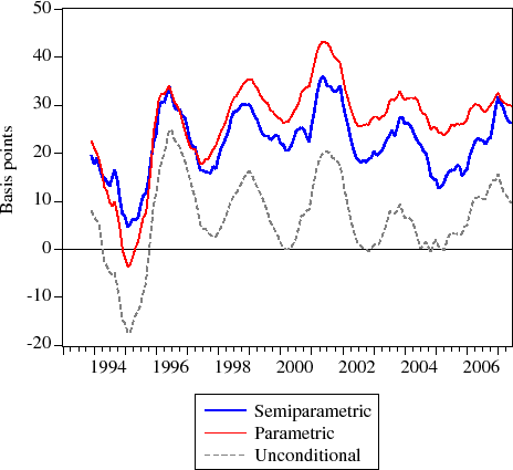
For each month of the MIRS data, I estimate the benchmark parametric model and the semiparametric partial local-linear regression model.¹¹ Figure 4 shows the 12-month moving averages for the two estimated time series of the jumbo-conforming spread as well as the unconditional jumbo-conforming spread, while Table 5 shows some sample statistics. As shown, the estimated jumbo-conforming spread series vary considerably during the January 1993 to June 2007 period. On average, the estimated jumbo-conforming spread under the parametric approach (27 basis points) is nearly 20 percent higher than under the semiparametric approach (22 basis points), and about 24 percent higher since 1996. This difference rises to as much as 75 percent in 2004. Both sets of estimates consistently exceed the unconditional difference between jumbo and conforming mortgage rates.

Of particular note is how the 12-month moving averages tend to track each other closely up until about 1996. Then the two series appear to drift apart permanently. One possible explanation for this is the widespread introduction of credit scoring in mortgage underwriting. In particular, the inclusion of credit scores in mortgage underwriting processes started around the end of 1995. Because the jumbo-conforming spread is estimated to be smaller when geography is included in the conditioning set, homeowners right at the conforming loan limit might have better credit quality than homeowners just above the conforming loan limit. For instance, a borrower who has the resources available to lower his or her loan size or LTV (perhaps as a signal on his or her credit worthiness) might have better credit quality than a borrower who does not have the resources available to lower his or her loan size or LTV. It could also be the case that jumbo borrowers no longer need to signal their credit quality through their loan-to-value ratios and jumbo-conforming status; now they can signal their credit quality through their credit scores. In either case, controlling for (unobserved) credit quality would tend to lower estimates of the jumbo-conforming spread, relative to an approach without such a control, as the effect would be separately identified from the jumbo-conforming spread.

Table 5 shows the average parameter estimates across time for each of the estimated models. Note that the average estimated effect of jumbo status on mortgage rates is positive (22 basis points), as are the effects of fees paid at closing (7 basis pints), whether the mortgage was originated by a mortgage company (9 basis points), whether the home was new (7 basis points), as well as state laws pertaining to whether judicial foreclosure is required (2 basis points) and whether deficiency judgments are prohibited (6 basis points). In the parametric specifications, loan size and the LTV ratio also have fairly substantial effects on mortgage rates (these effects are implicit in the semiparametric estimates). Of particular note are the average -squared values. The benchmark parametric model explains only about 11 percent of the variation in mortgage rates, on average. Without state-level foreclosure and ZIP-level demographic variables, the average -squared falls to around 8 percent. But for the semiparametric model the average -squared increases to over 61 percent, presumably reflecting nonlinearities of in and unobserved borrower and market characteristics that vary over geographic location.

Table 5 shows the parameter estimates for July 2005, as a particular example. The estimated effect of jumbo status on mortgage rates is statistically significant and positive (24 basis points), as are the effects of mortgage company origination (11 basis points), fees paid at closing (8 basis points), and new homes (20 basis points). In the parametric specifications, loan size and the LTV ratio again have statistically significant effects on mortgage rates. The same pattern also emerges with respect to the measure of fit: The semiparametric model dominates the benchmark parametric model.

At this point, several extensions deserve additional consideration. First, outside of [Ambrose, LaCour-Little, and SandersAmbrose et al.2004], the literature has largely ignored the potential endogeneity of loan size and LTV (and thus sample selection in jumbo status). In the parametric setting at least, procedures already exist to address these issues. The following subsections take a first pass at exploring these issues in the semiparametric context. Finally, estimates of the jumbo-conforming spread might vary across geographic locations. Thus, estimating the jumbo-conforming spread for specific geographies could prove to be an interesting exercise.

4a Endogeneity

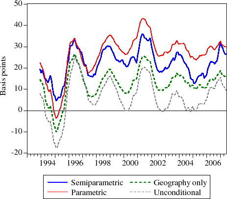
As noted above, estimates of the jumbo-conforming spread to this point have largely ignored the potential endogeneity of loan size and the loan-to-value ratio--i.e., the ability of certain borrowers to choose loan sizes and LTV ratios in order to secure conforming mortgage status (be it due to perceived price differences or to signaling good credit quality)--and the resulting sample selection of jumbo status. Thus, this section considers a semiparametric model that conditions only on geographic location (i.e., in equation 3). Now loans are compared only on the basis of how physically close they are and not on how they compare in loan size and loan-to-value ratio.

In addition, I estimate a nonparametric sample selection equation using jumbo mortgage status as the dependent variable and as the conditioning set. This essentially estimates the proportion of jumbo mortgages for any particular ZIP code and assumes that one borrower's jumbo-conforming status depends on his or her neighbors' jumbo-conforming status. Then, inserting the estimated inverse Mills ratio as an additional regressor in equation 3, we can evaluate the estimated effect of sample selection on mortgage rates.

As shown in Figure 5, controlling for the potential endogeneity of loan size and LTV and sample selection in jumbo status reduces the average estimate of the jumbo-conforming spread to about 13 basis points--a difference of over 40 percent from the original semiparametric model and a difference of nearly 50 percent from the benchmark parametric model. However, this estimate is not as low as the unconditional difference between jumbo and conforming mortgage rates, which averages 7 basis points over the 1993-2007 period. Further, contrary to the results reported in [Ambrose, LaCour-Little, and SandersAmbrose et al.2004], the estimated coefficient on the inverse Mills ratio is consistently small and statistically insignificant across time using these data and these methods.¹²

4b State-Level Estimates

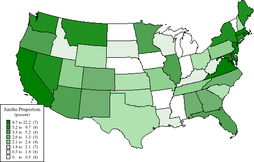
Figure 6 shows how the concentration of jumbo mortgages varies from state to state during June and July 2005. In general, fewer jumbo mortgages were originated in the middle of the country with the vast majority of jumbo mortgages being originated in coastal states. Within these data, the highest concentration of jumbo mortgage originations occurred in Washington DC, California, Maryland, Rhode Island, Virginia, Massachusetts, and New Jersey, while no jumbo mortgages were originated in Arkansas, Iowa, Mississippi, Nebraska, North Dakota, and Vermont during this period. With this in mind, how does the jumbo-conforming spread vary across states?

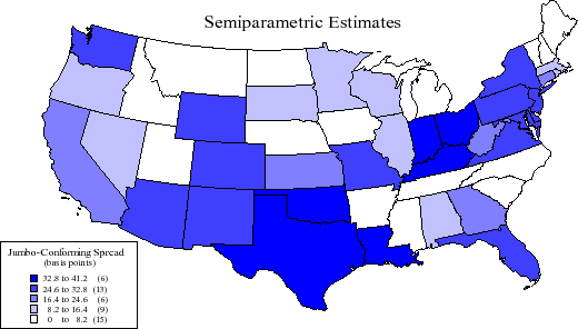
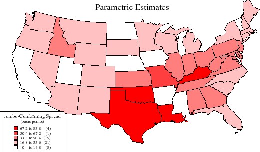
To answer this, I estimate the models for each state.¹³ As shown in Figure 7, semiparametric estimates of the jumbo-conforming spread were close to zero in 15 states and in excess of 33 basis points in 6 states. The national average was 24 basis points. Parametric estimates of the jumbo-conforming spread, in contrast, were near zero in 8 states and exceeded 33 basis points in 20 states. Here, the national average was 33 basis points. So the jumbo-conforming does indeed appear to vary by state, possibly reflecting further unobserved borrower or local market characteristics. Interestingly, there is no obvious correlation between the concentration of jumbo mortgages originated and the estimated jumbo-conforming spread across states.

5 Conclusion

This paper estimates the jumbo-conforming spread using data from the Federal Housing Finance Board's Monthly Interest Rate Survey from January 1993 to June 2007. Importantly, this paper augments the typical parametric approach by adding state-level foreclosure laws and ZIP-level demographic variables to the model, estimating the effects of loan size and loan-to-value ratio on mortgage rates nonparametrically, and including geographic location as a control for some potentially unobserved borrower and market characteristics that might vary over geography, such as credit scores, debt-to-income ratios, and house price volatility. A partial local-linear regression approach is used to estimate the jumbo-conforming spread, on the premise that loans similar to each other in terms of loan size, loan-to-value ratio, or geographic location might also be similar in other, unobservable borrower and market characteristics. I find estimates of the jumbo-conforming spread to be 13 to 24 basis points--50 to 24 percent smaller since about 1996, when credit scores became widely used in mortgage underwriting, than estimates from a commonly used parametric model. I therefore attribute the difference in estimates to credit quality and other unobserved characteristics, among other potential explanations, making these controls an important issue in estimating the jumbo-conforming spread.

Bibliography

Ambrose, B., M. LaCour-Little, and A. Sanders, (2004)

The effect of conforming loan status on mortgage yield spreads: A loan level analysis.
Real Estate Economics 32, 541-69.

Ambrose, B. W., R. Buttimer, and T. Thibodeau, (2001)

A new spin on the jumbo/conforming loan rate differential.
Journal of Real Estate Finance and Economics 23, 309-35.

Cotterman, R. F. and J. E. Pearce, (1996)

Studies on Privatizing Fannie Mae and Freddie Mac, Chapter The Effects of the Federal National Mortgage Association and the Federal Home Loan Mortgage Corporation on Conventional Fixed-Rate Mortgage Yields, pp. 97-168.
U.S. Department of Housing and Urban Development, Office of Policy Development and Research.

Hahn, J., P. Todd, and W. Van der Klaauw, (2001)

Identification and estimation of treatment effects with a regression-discontinuity design.
Econometrica 69, 201-9.

Hendershott, P. H. and J. D. Shilling, (1989)

The impact of the agencies on conventional fixed-rate mortgage yields.
Journal of Real Estate Finance and Economics 2, 101-15.

Lehnert, A., W. Passmore, and S. M. Sherlund, (2008)

GSEs, mortgage rates, and secondary market activities.
Forthcoming in Journal of Real Estate Finance and Economics.

McKenzie, J., (2002)

A reconsideration of the jumbo/non-jumbo mortgage rate differential.
Journal of Real Estate Finance and Economics 25, 197-214.

Naranjo, A. and A. Toevs, (2002)

The effects of purchases of mortgages and securitization by government sponsored enterprises on mortgage yield spreads and volatility.
Journal of Real Estate Finance and Economics 25, 173-96.

Pagan, A. and A. Ullah, (1999)

Nonparametric Econometrics.
Cambridge, UK: Cambridge University Press.

Passmore, W., S. M. Sherlund, and G. Burgess, (2005)

The effect of housing government-sponsored enterprises on mortgage rates.
Real Estate Economics 33, 427-63.

Passmore, W., R. Sparks, and J. Ingpen, (2002)

GSEs, mortgage rates, and the long-run effects of mortgage securitization.
Journal of Real Estate Finance and Economics 25, 215-42.

Pence, K. M., (2006)

Foreclosing on opportunity: State laws and mortgage credit.
Review of Economics and Statistics 88, 177-82.

Porter, J. R., (2002)

Asymptotic bias and optimal convergence rates for semiparametric kernel estimation in the regression discontinuity model.
Discussion Paper No. 1989, Harvard Institute of Economic Research, Harvard University, Cambridge MA.

Robinson, P. M., (1988)

Root-

-consistent semiparametric regression.
Econometrica 56, 931-54.

Silverman, B., (1986)

Density Estimation for Statistics and Data Analysis.
New York, NY: Chapman and Hall.

U.S. Congressional Budget Office (CBO), (2001)

Interest rate differentials between jumbo and conforming mortgages.
http://www.cbo.gov.

**Figure 1:** 30-Year Fixed-Rate Mortgage Rates

Note. January 1993 to June 2007.

**Figure 2:** 2006 Loan Size Distribution

Note. Normal (Gaussian) kernel density with bandwidth of $5000.

**Figure 3:** 2006 Loan Size Distribution

Note. Empirical cumulative distribution function.

**Figure 4:** Jumbo-Conforming Spread Estimates

Note. 12-month moving average.

**Figure 5:** Jumbo-Conforming Spread Estimates

Note. 12-month moving average.

**Figure 6:** Jumbo Mortgage Originations by State

Note. June-July 2005.

**Figure 7:** Jumbo-Conforming Spread Estimates by State

Note. June-July 2005.

Table 1: Jumbo-Conforming Spread
	Mean	Median	Std.Dev.	Minimum	Maximum	Correlation
Total Semiparametric	22.23	22.83	13.49	-30.74	57.93	.7291
Total Parametric	26.53	27.53	12.76	-44.77	62.26
1993 Semiparametric	19.64	17.88	11.47	-5.41	35.76	.3099
1993 Parametric	22.60	24.08	10.14	9.71	36.52
1994 Semiparametric	7.24	7.87	18.79	-30.74	32.94	.7415
1994 Parametric	-0.25	5.95	20.69	-44.77	23.95
1995 Semiparametric	22.26	23.55	17.45	-14.89	55.28	.8130
1995 Parametric	24.53	27.03	15.00	-3.85	41.49
1996 Semiparametric	27.51	27.27	12.45	6.40	50.12	.7360
1996 Parametric	24.83	21.54	8.68	15.17	39.71
1997 Semiparametric	16.71	16.03	8.15	2.53	29.34	.8453
1997 Parametric	21.55	22.64	6.30	11.80	31.59
1998 Semiparametric	30.06	30.93	7.03	11.66	38.76	.5107
1998 Parametric	35.20	34.68	3.42	30.36	41.15
1999 Semiparametric	23.60	24.16	8.98	9.25	38.55	.7478
1999 Parametric	27.40	25.50	6.47	18.42	38.19
2000 Semiparametric	22.35	22.02	14.14	-5.64	43.96	.5880
2000 arametric	33.95	34.63	7.13	24.56	47.65
2001 Semiparametric	34.18	31.83	15.55	5.27	57.93	.9546
2001 Parametric	38.79	34.72	12.72	18.50	62.26
2002 Semiparametric	19.13	17.87	7.93	9.82	30.85	.5376
2002 Parametric	27.10	28.19	5.59	18.47	32.88
2003 Semiparametric	27.53	24.97	12.47	10.19	56.73	.7550
2003 Parametric	31.74	29.79	9.72	17.77	47.55
2004 Semiparametric	14.59	15.39	6.55	2.71	23.77	.4686
2004 Parametric	25.49	24.83	2.35	22.14	28.96
2005 Semiparametric	16.10	19.30	9.37	-3.36	25.94	.4607
2005 Parametric	26.33	26.03	5.27	16.60	37.62
2006 Semiparametric	29.47	33.62	11.75	9.44	51.53	.6501
2006 Parametric	31.85	31.09	6.16	22.38	41.66
2007 Semiparametric	23.90	21.06	10.11	15.88	43.83	.9439
2007 Parametric	27.04	24.24	7.19	22.64	41.54

Table 2: Average Parameter Estimates for 1993-2007
	Semiparametric	Parametric (1)	Parametric (2)
Constant	-0.0019	9.0605	8.6741
Jumbo mortgage	0.2223	0.2695	0.2653
$\ln(Size_i)$	--	-0.1652	-0.1644
$LTV_i \le 75$	--	-0.0069	-0.0121
$80 < LTV_i \le 90$	--	0.1164	0.1127
	--	0.0567	0.0575
Mortgage company	0.0888	0.0763	0.0904
Fees paid	0.0700	0.0647	0.0649
New home	0.0674	0.0509	0.0512
Urban pop. share	-0.0004	--	-0.0005
Suburban pop. share	-0.0002	--	-0.0001
Black pop. share	0.0008	--	0.0003
Asian pop. share	-0.0001	--	0.0011
Hisp. pop. share	0.0004	--	0.0020
Age 0-9 pop. share	0.0004	--	0.0002
Age 10-17 pop. share	0.0012	--	0.0008
Age 18-21 pop. share	0.0002	--	-0.0029
Age 22-29 pop. share	0.0017	--	0.0000
Age 40-49 pop. share	0.0014	--	-0.0004
Age 50-59 pop. share	0.0022	--	-0.0002
Age 60-69 pop. share	0.0021	--	0.0021
Age 70-79 pop. share	0.0000	--	0.0004
Age 80+ pop. share	0.0005	--	0.0020
Edu. 9 pop. share	-0.0007	--	-0.0047
Edu. 9-12 pop. share	-0.0002	--	0.0011
Edu. coll. pop. share	0.0010	--	0.0030
Edu. Assoc. pop. share	-0.0039	--	0.0011
Edu. Bach. pop. share	-0.0010	--	-0.0055
Edu. Prof. pop. share	-0.0014	--	0.0018
$\ln(Income)$	0.0012	--	-0.0288
$\ln(House \; value)$	0.0033	--	0.0576
Judicial foreclosure	0.0152	--	0.0211
Right of redemption	0.0040	--	0.0017
Deficiency judgment	0.0584	--	0.0110
-squared	0.6144	0.0824	0.1110

Table 3: Parameter Estimates for July 2005
	Semiparametric	Parametric (1)	Parametric (2)
Constant	-0.0033 *	8.3491 *	8.3885 *
Constant (standard error)	(.0011)	(.2066)	(.7236)
Jumbo mortgage	0.2387 *	0.3896 *	0.3762 *
Jumbo mortgage (standard error)	(.0566)	(.0331)	(.0305)
$\ln(Size_i)$	--	-0.2220 *	-0.2037 *
$\ln(Size_i)$ (standard error)		(.0170)	(.0180)
$LTV_i \le 75$	--	-0.0618 *	-0.0617 *
$LTV_i \le 75$ (standard error)		(.0155)	(.0149)
$80 < LTV_i \le 90$	--	0.3299 *	0.3061 *
$80 < LTV_i \le 90$ (standard error)		(.0344)	(.0329)
	--	0.0527 *	0.0366
(standard error)		(.0215)	(.0208)
Mortgage company	0.1062 *	0.1206 *	0.1327 *
Mortgage company (standard error)	(.0174)	(.0172)	(.0137)
Fees paid	0.0825 *	0.0664 *	0.0704 *
Fees paid (standard error)	(.0122)	(.0171)	(.0143)
New home	0.1987 *	0.2321 *	0.2314 *
New home (standard error)	(.0189)	(.0236)	(.0215)
Urban pop. share	0.0003	--	0.0000
Urban pop. share (standard error)	(.0003)		(.0003)
Suburban pop. share	0.0013 *	--	0.0012 *
Suburban pop. share (standard error)	(.0004)		(.0004)
Black pop. share	0.0004	--	0.0012
Black pop. share (standard error)	(.0008)		(.0007)
Asian pop. share	-0.0024	--	0.0000
Asian pop. share (standard error)	(.0014)		(.0019)
Hisp. pop. share	0.0009	--	0.0032 *
Hisp. pop. share (standard error)	(.0012)		(.0010)
Age 0-9 pop. share	-0.0053	--	-0.0086
Age 0-9 pop. share (standard error)	(.0065)		(.0056)
Age 10-17 pop. share	-0.0001	--	-0.0001
Age 10-17 pop. share (standard error)	(.0058)		(.0046)
Age 18-21 pop. share	-0.0001	--	-0.0050
Age 18-21 pop. share (standard error)	(.0041)		(.0039)
Age 22-29 pop. share	-0.0049	--	-0.0066
Age 22-29 pop. share (standard error)	(.0068)		(.0050)
Age 40-49 pop. share	0.0030	--	0.0010
Age 40-49 pop. share (standard error)	(.0052)		(.0050)
Age 50-59 pop. share	-0.0077	--	-0.0096 *
Age 50-59 pop. share (standard error)	(.0055)		(.0047)
Age 60-69 pop. share	0.0091	--	0.0064
Age 60-69 pop. share (standard error)	(.0065)		(.0067)
Age 70-79 pop. share	-0.0107 *	--	-0.0040
Age 70-79 pop. share (standard error)	(.0053)		(.0062)
Age 80+ pop. share	0.0032	--	0.0005
Age 80+ pop. share (standard error)	(.0065)		(.0059)
Edu. 9 pop. share	0.0064	--	-0.0060
Edu. 9 pop. share (standard error)	(.0055)		(.0052)
Edu. 9-12 pop. share	-0.0013	--	0.0102 *
Edu. 9-12 pop. share (standard error)	(.0057)		(.0042)
Edu. coll. pop. share	0.0013	--	0.0038
Edu. coll. pop. share (standard error)	(.0041)		(.0034)
Edu. Assoc. pop. share	0.0004	--	-0.0050
Edu. Assoc. pop. share (standard error)	(.0068)		(.0051)
Edu. Bach. pop. share	-0.0046	--	-0.0009
Edu. Bach. pop. share (standard error)	(.0031)		(.0032)
Edu. Prof. pop. share	0.0007	--	0.0048
Edu. Prof. pop. share (standard error)	(.0033)		(.0031)
$\ln(Income)$	0.0347	--	0.0116
$\ln(Income)$ (standard error)	(.0779)		(.0590)
$\ln(House \; value)$	-0.0049	--	-0.0231
$\ln(House \; value)$ (standard error)	(.0380)		(.0312)
Judicial foreclosure	-0.0116	--	0.0237
Judicial foreclosure (standard error)	(.0346)		(.0174)
Right of redemption	0.2287 *	--	-0.0928 *
Right of redemption (standard error)	(.0593)		(.0319)
Deficiency judgment	-0.1123	--	-0.0321 *
Deficiency judgment	(.1163)		(.0191)
-squared	0.6636	0.1213	0.1404

Bootstrap standard errors in parentheses.

* = statistically significant at 95 percent confidence level.

Footnotes

1. I thank Brent Ambrose, Brian Bucks, Karen Dynan, Wayne Passmore, Karen Pence and seminar participants at the Federal Reserve Board and the 2007 AREUEA Annual Meetings for helpful comments and suggestions. This paper represents the views of the author and does not necessarily represent the views of the Federal Reserve Board, its members, or its staff. Return to Text

2. Using time-series data from 1993 to 2005, [Lehnert, Passmore, and SherlundLehnert et al.2008] find that GSE portfolio purchases have no effect on mortgage rates. Return to Text

3. Conforming loans have stricter underwriting requirements than nonconforming loans, whereas jumbo loans have loan sizes above the conforming loan limit. Return to Text

4. Over this period, the MIRS data contain observations on over 3.4 million total mortgage originations. Of these, 908 thousand are adjustable-rate mortgages, 506 thousand have terms other than 30 years, 39 thousand have invalid or missing ZIP codes, 11 thousand are from Alaska or Hawaii, 11 thousand have LTV ratios less than 20 percent or greater than 100 percent, 22 thousand have loan amounts smaller than 1/8th the conforming loan limit, and less than 1 thousand violated the mortgage rate filter. Return to Text

5. Classifications include $LTV_i \le 75$ , $75 < LTV_i \le 80$ (excluded), $80 < LTV_i \le 90$ , and

. Return to Text

6. Additional discontinuities include loan-to-value ratio, whether the mortgage had fees paid at closing, whether the mortgage was originated by a mortgage company, and whether the home was new. Return to Text

7. I relax this condition in section 4.1. Return to Text

8. Distances between ZIP code centroids are computed using the Haversine formula for great circle distances. Return to Text

9. Ideally, one would cross-validate the bandwidth parameters, but this proves to be computationally prohibitive in this application. I therefore use a rule-of-thumb bandwidth suggested by [SilvermanSilverman1986], $b_n=c \sigma_z n^{-1/(d+4)}$ , where $c=d^{1/(d+4)}(\frac{4}{2d+1})^{1/(d+4)}$ , $\sigma_z$ is the standard deviation of

, and $d=\dim(z_i)$ . Bandwidths range from 0.15 to 0.22 for $\ln(Size_i)$ , from 4.4 to 6.5 percentage points for

, and from 28 to 44 miles over geography. Return to Text

10. As with cross-validation of the bandwidth parameters, bootstrapping the standard errors of the parameter estimates is too computationally burdensome, although I show bootstrapped standard errors for one month, in particular, as an example. Return to Text

11. I also estimate a parametric model that excludes the state-level foreclosure and ZIP-level demographic variables to show how much power the nonparametric components add to the estimation, as opposed to the state- and ZIP-level variables. These estimates are similar to the benchmark parametric model's and thus are largely omitted. Return to Text

12. Estimates are available upon request. Return to Text

13. Because many cities span state lines, I include out-of-state observations within 100 miles of state boundaries in each state's individual estimation. Return to Text

^♣ This version is optimized for use by screen readers. Descriptions for all mathematical expressions are provided in LaTex format. A printable pdf version is available. Return to Text

The Jumbo-Conforming Spread: A Semiparametric Approach 1