Skip to: [Printable Version (PDF)] [Bibliography] [Footnotes]

Finance and Economics Discussion Series: 2008-15 Screen Reader version ^♣

Lack of Signal Error (LoSE) and Implications for OLS Regression: Measurement Error for Macro Data

Jeremy J. Nalewaik*

First Draft: October 2007

Keywords: Measurement error, regression, macroeconomic data

Abstract:

This paper proposes a simple generalization of the classical measurement error model, introducing new measurement errors that subtract signal from the true variable of interest, in addition to the usual classical measurement errors (CME) that add noise. The effect on OLS regression of these lack of signal errors (LoSE) is opposite the conventional wisdom about CME: while CME in the explanatory variables causes attenuation bias, LoSE in the dependent variable, not the explanatory variables, causes a similar bias under some conditions. The paper provides evidence that LoSE is an important source of error in US macroeconomic quantity data such as GDP growth, illustrates downward bias in regressions of GDP growth on asset prices, and provides recommendations for econometric practice.

1 Introduction

This paper proposes a simple generalization of the classical measurement error model and studies its implications for ordinary least squares (OLS) regression. The usual model starts with the true variable of interest and adds noise, which we call classical measurement error (CME); see Klepper and Leamer (1984), Griliches (1986), Fuller (1987), Leamer (1987), Angrist and Krueger (1999), Bound, Brown and Mathiowetz (2001) or virtually any econometrics textbook. The generalization discussed here incorporates a different kind of measurement error that subtracts signal from the true variable; this new error term is called the Lack of Signal Error, or LoSE for short. This additional term adds some much-needed flexibility to the classical measurement error model: it allows the mismeasured variable to have either more or less variance than the true variable of interest, in contrast to the classical model, which imposes that the mismeasured variable has higher variance. This restriction does not hold in some important applications in macroeconomics and elsewhere.

The implications of LoSE for OLS regression are opposite the usual intuition about measurement error, which is applicable to CME only. The CME intuition says that measurement error in the dependent variable of a regression poses no real problems for standard estimation and inference. Parameter estimates are unbiased and consistent, while hypotheses are more difficult to reject because CME increases the variance of regression residuals and thus standard errors. CME in the explanatory variables causes the real problems for OLS regression, namely attenuation bias and inconsistency. However with LoSE these results are reversed. For the baseline case considered here, LoSE in the explanatory variables produces no bias or inconsistency while increasing standard errors, similar to CME in . It is LoSE in the dependent variable that introduces an attenuation-type bias and inconsistency into the regression under some circumstances (in particular, when the explanatory variables contain some signal missing from the dependent variable). This point is obvious when we consider the extreme case of maximum LoSE in , so is just a constant equal to its unconditional mean. Then a standard OLS regression of on any explanatory variable with positive variance recovers $\widehat{\beta} = \frac{\mathop{\mathrm{cov}}(X,Y)}{\mathop{\mathrm{var}}(X)} = 0$ , regardless of the true $\beta$ . In addition, LoSE in shrinks the variance of regression residuals, thus shrinking parameter standard errors compared to what they would be without this type of mismeasurement. The standard errors are zero in our extreme case, and this raises concerns about the robustness of hypothesis tests.

Much of the econometrics literature on non-classical measurement error has focused on binary or categorical response data, for which the classical measurement error assumptions cannot hold; see Card (1996), Bollinger (1996), and Kane, Rouse and Staiger (1999). In a more general linear regression context, Berkson (1950) was an early paper tackling some of the issues addressed here; see the discussion in Durbin (1954), Griliches (1986, section 4), and Fuller (1987, section 1.6.4). Berkson had in mind a regression using "controlled" measurements as the explanatory variable , readings from a scientific experiment where the unobserved true values of interest $X^\star$ fluctuate around the observed controlled measurements in a random way. Berkson showed that if the unobserved fluctuations $X^\star-X$ are uncorrelated with the measurements , then regression parameter estimates are unbiased. The literature following Berkson has generally focused on extending his results to regressions employing non-linear functions of ; see Geary (1953), Federov (1974), Carroll and Stefanski (1990), Huwang and Huang (2000), and Wang (2003, 2004). This literature has focused less on the implications of "controlled" measurements of the dependent variable .

Other papers discussing different LoSE-related estimation issues include Sargent (1989), Bound, Brown and Mathiowetz (2001), and Kimball, Sahm and Shapiro (2008). Perhaps the closest paper to this one is Hyslop and Imbens (2001), which shows some of the major implications of LoSE, while simultaneously considering the implications of a different problem, correlation between the measurement error in and the regression error. In defining the LoSE in a variable as the difference between its true value and a conditional expectation of that true value, we consider arbitrary conditioning information sets ; Hyslop and Imbens (2001) consider information sets consisting of only mismeasured and mismeasured in a univariate regression context. Considering general information sets allows us to derive more general results, clarifying under what conditions LoSE produces attenuation bias and what instruments are valid in addressing that bias.

A large body of empirical work has now accumulated on mismeasurement of microeconomic survey data, which generally rejects the CME assumptions and points to negative correlation between the measurement errors and the true variables of interest; see Bound and Krueger (1991), Bound, Brown, Duncan and Rodgers (1994), Pishcke (1995), Bollinger (1998), Bound, Brown and Mathiowetz (2001) and the references therein, and Escobal and Laszlo (2008). Such negative correlation is an implication of LoSE, although other measurement error models may generate such a result as well. The empirical work in this paper focuses on a different type of data, namely US macroeconomic quantity data such as gross domestic product (GDP) and gross domestic income (GDI). These data pass through numerous revisions, and the more poorly-measured initial estimates have less variance than the revised estimates, providing a concrete example of measurement error that cannot be CME; see Mankiw and Shapiro (1986).

After providing a brief introductory motivation for the generalized measurement error model in Section 2 and showing the implications for OLS regression in Section 3, Section 4.1 of the paper discusses the nature of the source data used to compute US macroeconomic quantity data, and points out some reasons why LoSE may be present in the estimates even after they have passed through all their revisions. GDP growth and GDI growth measure the same underlying concept, but use different source data; see Fixler and Nalewaik (2007) and Nalewaik (2007a). Since the two measures are far from equal in the fully-revised quarterly or annual frequency data, some mismeasurement must remain in either GDP or GDI growth. Section 4.2 reviews the evidence in Fixler and Nalewaik (2007) and Nalewaik (2007a,b) supporting the notion that this mismeasurement is largely LoSE in GDP growth. Some simple calculations comparing GDP and GDI growth show that this LoSE in GDP growth is likely substantial: after 1984, at least 30% of the variance of the true growth rate of the economy appears to be missing.

In a wide variety of econometric specifications employed in the macroeconomics and finance, variables like GDP growth, investment growth and consumption growth are regressed on asset prices - interest rates, stock price changes, exchange rate changes, etc. These regressions are of particular interest because asset prices potentially capture some signal missing from the mismeasured quantities, implying attenuation-type biases in the coefficients. Section 4.3 tests for these biases, regressing output growth measures contaminated with different degrees of LoSE on a fixed set of stock or bond prices. In cases where we suspect the dependent variable is contaminated with more LoSE, the regression coefficients are smaller, and the differences across regressions are often statistically significant. For example, the coefficients increase when we switch the dependent variable from the early GDP growth estimates based on limited source data to later GDP growth estimates based on more-comprehensive data. Tellingly, the coefficients increase again when we switch the dependent variable from GDP growth to GDI growth. The hypothesis that measurement error in the dependent variable does not bias OLS regression coefficients, a core piece of conventional wisdom in the profession, is rejected by the data, just as the paper predicts if the measurement error is LoSE.

Section 5 concludes the paper with a review of some of the major implications of substantial LoSE in GDP growth. Implications for econometric practice are discussed, using examples of popular regressions in macroeconomics.

2 A Generalization of the Classical Measurement Error Model

Let $Y_t^\star$ be the true value of the variable of interest, be a mismeasured estimate of that variable, and be a $\left(1 \times l \right)$ vector of possibly stochastic variables used to construct . In many cases a government statistical agency or some other organization computes based on information from surveys, administrative records, and other data sources (source data for short); then will be variables drawn from the source data, possibly including non-linear functions of the original source data.

Under the classical measurement error model,

$\displaystyle Y_t$

$\displaystyle =$

$\displaystyle Y_t^\star + \varepsilon_t.$

The term $\varepsilon_t$ is "noise" or the classical measurement error (CME) in the estimate. In the current context this is taken to imply independence of $\varepsilon_t$ and $Y_t^\star$ , although the weaker assumption $\mathop{\mathrm{cov}}\left(Y_t^\star,\varepsilon_t\right) = 0$ suffices for many purposes. The CME may arise from estimation errors or other sources; since many estimates

are based on surveys, survey sampling errors are often thought to be a source of CME.

Under the generalized model of mismeasurement considered here, the mismeasured estimate is as in Fixler and Nalewaik (2007):

$\displaystyle Y_t$

$\displaystyle =$

$\displaystyle E\left(Y_t^\star \vert Z_t \right) + \varepsilon_t.$

(1)

The CME term $\varepsilon_t$ is assumed independent of

and $Y_t^\star$ . It can be seen immediately that the classical measurement error model is a special case of this more general model, where

spans $Y_t^\star$ so $E\left(Y_t^\star \vert Z_t \right) = Y_t^\star$ .

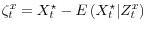
Define the deviation of the variable of interest from its conditional expectation as:

$\displaystyle \zeta_t$

$\displaystyle =$

$\displaystyle Y_t^\star - E\left(Y_t^\star \vert Z_t \right).$

(2)

This deviation represents the information about $Y_t^\star$ not contained in

, and is uncorrelated with all functions of

. With $\mathop{\mathrm{cov}}\left(E\left(Y_t^\star \vert Z_t \right),\zeta_t\right) = 0$ , the variance of the true variable of interest may be decomposed into the variance of the conditional expectation plus the variance of $\zeta_t$ , and: $\mathop{\mathrm{var}}\left(\zeta_t\right) = \mathop{\mathrm{var}}\left(Y_t^\star\right) - \mathop{\mathrm{var}}\left(E\left(Y_t^\star \vert Z_t \right)\right)$ . The variance of $\zeta_t$ represents the variance of the information about $Y_t^\star$ missing from the conditional expectation. Substituting into (1):

$\displaystyle Y_t$

$\displaystyle =$

$\displaystyle Y_t^\star - \zeta_t + \varepsilon_t.$

(3)

Thinking of $\varepsilon_t$ as mismeasurement from noise, $\zeta_t$ represents an opposite kind of mismeasurement, mismeasurement from lack of signal about $Y_t^\star$ in the information used to construct

. As such, $\zeta_t$ may be labelled the Lack of Signal Error, or LoSE for short.

Taking variances of (3), the LoSE is clearly correlated with $Y_t^\star$ , with $\mathop{\mathrm{cov}}\left(Y_t^\star,\zeta_t\right) = \mathop{\mathrm{var}}\left(\zeta_t\right)$ in fact, so:

$\displaystyle \mathop{\mathrm{var}}\left(Y_t\right)$	$\displaystyle =$	$\displaystyle \mathop{\mathrm{var}}\left(Y_t^\star\right) + \mathop{\mathrm{var}}\left(\zeta_t\right) - 2\mathop{\mathrm{cov}}\left(Y_t^\star,\zeta_t\right) + \mathop{\mathrm{var}}\left(\varepsilon_t\right)$
	$\displaystyle =$	$\displaystyle \mathop{\mathrm{var}}\left(Y_t^\star\right) - \mathop{\mathrm{var}}\left(\zeta_t\right) + \mathop{\mathrm{var}}\left(\varepsilon_t\right).$	(4)

Depending on whether the variance of the LoSE is greater than or less than the variance of the CME, the variance of the estimate

may be greater than or less than the variance of the true variable of interest $Y_t^\star$ . With CME alone, the variance of the estimate

must exceed the variance of the true variable. The key limitation of the CME model is the assumption that $\mathop{\mathrm{cov}}\left(Y_t - Y_t^\star, Y_t^\star \right) = 0$ . It is easy to think of theoretical counterexamples, for example, when $Y_t^\star$ has positive variance but the estimate

is just a constant for all

; actual counterexamples are provided in the introduction and section 4. The generalization with LoSE allows this covariance to range from 0 to a lower bound of negative $\mathop{\mathrm{var}}\left(Y_t - Y_t^\star \right)$ , in which case all the mismeasurement arises from LoSE.

While the generalized model here is less restrictive than the CME model, some restrictions do remain. Writing:

$\displaystyle Y_t + \zeta_t$

$\displaystyle =$

$\displaystyle Y_t^\star + \varepsilon_t,$

(5)

the zero covariance between $\zeta_t$ from

is a restriction, implied by the first term on the right of (1) being a conditional expectation. Systematic biases in the estimate, on top of those caused by noise,¹ violate this assumption. For concreteness, assume $E\left(Y_t^\star \vert Z_t \right) = Z_t\gamma$ . Consider an estimate of $Y^{\star}_t$ based on

that misuses the information, so $Y_t = Z_t\widetilde{\gamma} + \varepsilon_t$ with $\widetilde{\gamma} \neq \gamma$ . The estimate "misses" in a systematic way. For estimation and inference about $Y_t^\star$ and its relation to other variables (for example in attempting to estimate $\beta$ by OLS in the relation $Y_t^\star = X_t^\star\beta +U_t^\star$ using the mismeasured data), these "misses" clearly lead to biased and inconsistent estimates. However unless additional information is available about the nature of $Z_t \widetilde{\gamma} - Z_t\gamma$ , the direction and magnitude of these biases is unclear. In highly stylized examples, the biases may be derived; one such example is $Y_t = \alpha_0 + \alpha_1 Y_t^{\star} + \varepsilon_t$ , with $\alpha_0 \ne 0$ and $\alpha_1 \ne 1$ ; this model is employed by de Leeuw and McKelvey (1983), Bound, Brown, Duncan and Rodgers (1994), Piscke (1995), and Bound, Brown and Mathiowetz (2001). But once one allows for these systematic biases in the estimates, there is generally no reason to prefer one highly stylized example to another, and we are in a wilderness of possibilities.

In the case of GDP and GDI growth, the model $Y_t = \alpha_0 + \alpha_1 Y_t^{\star} + \varepsilon_t$ does not fit the facts, as the discussion of table 3A and 3B in section 4.3 makes clear. In general, an important goal of all creators of data (government statistical agencies as well as other groups) is to avoid systematic mismeasurement like that described in the previous paragraph. Indeed, their ultimate goal is probably to produce estimates that are as close as possible to $E\left(Y_t^\star \vert Z_t \right)$ , with as broad an information set as possible given resource constraints. As such, the generalized model (1) is a useful benchmark, and should approximate well the underlying mismeasurement in many situations. It also has the advantage of being mathematically tractable, and the symmetry between adding noise and subtracting signal is intuitive and appealing.

Before concluding this section, it is worth emphasizing that need not be an exhaustive information set - i.e. it need not contain all available relevant pieces of information about unobserved $Y_t^\star$ . Resource and other constraints certainly preclude this from being the case, and the sections below considering the implications of LoSE allow for this possibility.

3 Implications for OLS Estimation

Consider ordinary least squares estimation of the relation between a mismeasured variable and a $\left(1 \times k \right)$ set of mismeasured explanatory variables , using a sample of length . When stacking together the observations, time subscripts are dropped for convenience:

$\begin{displaymath}\begin{array}{cc} Y = \left(\begin{array}{c} Y_{1} \\ Y_{2} \\ \vdots \\ Y_{T} \end{array}\right); & X = \left(\begin{array}{c} X_{1} \\ X_{2} \\ \vdots \\ X_{T} \end{array}\right). \end{array}\end{displaymath}$

Our full set of assumptions follows:

Assumption 1 $Y_t^\star = X_t^\star\beta +U_t^\star$ . $U_t^\star$ is i.i.d., mean zero, with $\mathop{\mathrm{var}}\left(U_t^\star\right) = \sigma^2_{U^\star}$ and $U_s^\star$ independent of $X_t^\star$ , $\forall t,s$ . Measured $Y_t = E\left(Y_t^\star \vert Z_t^y \right) + \varepsilon_t$ , with:

The CME $\varepsilon_t$ is i.i.d., mean zero, and independent of all conditioning information sets, with $\mathop{\mathrm{var}}\left(\varepsilon_t\right) = \sigma^2_{\varepsilon}$ .
may be partitioned into two sets of variables, and , with variables in independent of $U^\star$ and , and variables in independent of $X^\star$ and .
The LoSE $\zeta_t = \left(X^\star_t - E\left(X^\star_t \vert Z_{x,t}^y \right)\right)\beta + U_t^\star - E\left(U_t^\star \vert Z_{u,t}^y \right) = \zeta_t^{xy}\beta + \zeta_t^u$ . $\zeta_t^u$ is i.i.d. and mean zero with $\mathop{\mathrm{var}}\left(\zeta_t^u\right) = \sigma^2_{\zeta,u}$ , and $\zeta_t^{xy}$ is i.i.d. and mean zero with $\mathop{\mathrm{var}}\left(\zeta_t^{xy}\right) = \sigma^2_{\zeta,xy}$ , a $k \times k$ matrix.

Measured $X_t = E\left(X_t^\star \vert Z_t^x \right) + \varepsilon_t^x$ , with:

The CME $\varepsilon_t^x$ is i.i.d., mean zero, independent of $\varepsilon_t$ and all conditioning information sets, with $\mathop{\mathrm{var}}\left(\varepsilon_t^x\right) = \sigma^2_{\varepsilon,x}$ , a $k \times k$ matrix.
The variables in are independent of $U^\star$ and .
The LoSE $\zeta_t^x = X_t^\star - E\left(X_t^\star \vert Z_t^x \right)$ is i.i.d. and mean zero with $\mathop{\mathrm{var}}\left(\zeta_t\right) = \sigma^2_{\zeta,x}$ , a $k \times k$ matrix.
As $T\longrightarrow \infty$ :
- $\frac{1}{T} \left(X^{\star}\right)^\prime X^{\star} \stackrel{p}{\longrightarrow} Q_{xx}$
- $\frac{1}{T} \left(E\left( X^\star \vert Z_x^y \right)\right) ^\prime E\left( X^\star \vert Z_x^y \right)\stackrel{p}{\longrightarrow} Q_{xx}^{zy} = Q_{xx} - \sigma^2_{\zeta,xy}$
- $\frac{1}{T} \left(E\left( X^\star \vert Z^x \right)\right) ^\prime E\left( X^\star \vert Z^x \right)\stackrel{p}{\longrightarrow} Q_{xx}^{zx} = Q_{xx} - \sigma^2_{\zeta,x}$
- $\frac{1}{T} \left(E\left( X^\star \vert Z_x^y \right)\right) ^\prime E\left( X^\star \vert Z^x \right)\stackrel{p}{\longrightarrow} Q_{xx}^{zb}$
- $\frac{1}{T} X^\prime X \stackrel{p}{\longrightarrow} = Q_{xx}^{zx} + \sigma^2_{\varepsilon,x}$ .

All relevant fourth moments exist.

For most purposes, especially for time series analysis, the i.i.d. and homoskedasticity assumptions here are overly restrictive, but relaxing them is straightforward; we keep these assumptions so we may discuss bias as well as consistency.

The assumptions imposed on the information sets and regarding partitioning and independence allow us to factor the joint distribution of the relevant variables as follows:

$\displaystyle f\left( U^\star, X^\star, Z^y , Z^x \right)$

$\displaystyle =$

$\displaystyle f_{UZ}\left(U^\star, Z^y_u \right) f_{XZ}\left(X^\star, Z^y_x , Z^x \right).$

Without these assumptions, the conditioning may introduce correlation between the measurement error in

and the regression residual (which includes the measurement error in

). An example where the conditioning has this effect is in Hyslop and Imbens (2001). As another example, assume the information sets

, and

are univariate, and let

; then $E\left(X_t^\star \vert Z_t^x \right)$ and $\zeta_t^x$ are correlated with $U^\star$ (as long as

captures some variation in $U^\star$ ), and the above factorization is not valid. Correlation between the measurement error in the explanatory variables and the regression error can introduce serious biases in some regressions, but I view these biases as distinctly different from those introduced by Lack of Signal. To understand clearly the implications of LoSE, what biases it may introduce and under what conditions, isolating its effects from other biases is useful. Our assumptions allow us to do that.

Given assumption 1, can be written as:

$\displaystyle Y_t$	$\displaystyle =$	$\displaystyle E\left(X_t^\star\vert Z_{x,t}^y \right) \beta + E\left(U_t^\star \vert Z_{u,t}^y \right) + \varepsilon_t$	(6)
	$\displaystyle =$	$\displaystyle X_t\beta + \left(E\left(X_t^\star \vert Z_{x,t}^y \right) - X_t\right)\beta + E\left(U_t^\star \vert Z_{u,t}^y \right) + \varepsilon_t$
	$\displaystyle =$	$\displaystyle X_t\beta + \left(E\left(X_t^\star \vert Z_{x,t}^y \right) - E\left(X_t^\star \vert Z_t^x \right) - \varepsilon_t^x\right)\beta + U_t^\star - \zeta_t^u + \varepsilon_t.$

The OLS regression estimator is:

$\displaystyle \widehat{\beta}$	$\displaystyle =$	$\displaystyle \left( X^\prime X \right)^{-1} X^\prime Y$
	$\displaystyle =$	$\displaystyle \beta + \left( X^\prime X \right)^{-1} X^\prime \left(\left(E\left(X^\star \vert Z_x^y \right) - E\left(X^\star \vert Z^x \right) - \varepsilon^x\right)\beta + U^\star - \zeta^u + \varepsilon \right).$	(7)

Consider the sources of bias and inconsistency in this estimate. It is well known that the CME in

introduces no bias and inconsistency, since $\varepsilon$ is independent of

. Interestingly, the LoSE in $U^\star$ introduces no bias or inconsistency either: given the assumptions about the information sets, $E\left( U^\star \vert Z_u^y \right)= U^\star - \zeta^u$ is uncorrelated with $E\left(X^\star \vert Z^x \right)$ and hence $X = E\left(X^\star \vert Z^x \right) + \varepsilon^x$ . The other components in the error of (6) do cause bias and inconsistency; taking expectations and probability limits of (7) yields:

$\displaystyle E\left(\widehat{\beta}\right)$	$\displaystyle =$	$\displaystyle \beta + E\left(\left( X^\prime X \right)^{-1}X^\prime \left( E\left(X^\star \vert Z_x^y \right) - E\left(X^\star \vert Z^x \right) - \varepsilon^x \right) \right) \beta,$ and:	(8)
$\displaystyle \widehat{\beta}$	$\displaystyle \stackrel{p}{\longrightarrow}$	$\displaystyle \beta + \left(Q_{xx}^{zx} + \sigma^2_{\varepsilon,x}\right)^{-1} \left( Q_{xx}^{zb} - Q_{xx}^{zx} - \sigma^2_{\varepsilon,x} \right)\beta.$	(9)

The usual attenuation bias and inconsistency from CME in

is evident. The additional inconsistency from LoSE depend on the difference between $Q_{xx}^{zb}$ and $Q_{xx}^{zx}$ . Illuminating special cases are discussed in the subsections below, especially subsection 3.4, but clearly the correlation between the variables in

and

is critical here.

The inconsistency of $\widehat{\beta}$ can be corrected by instrumenting with a $\left(1 \times m \right)$ set of instruments , with $m \geq k$ , if the instruments meet the following set of assumptions:

Assumption 2 With $P_W = W \left(W^\prime W \right)^{-1}W^\prime$ , $\frac{1}{T}X^\prime P_W X \stackrel{p}{\longrightarrow} Q_{xx}^w$ , a positive semi-definite matrix, and $\frac{1}{T} X^\prime P_W \left( \left(E\left( X^\star \vert Z_x^y \right) - E\left( X^\star \vert Z^x \right) - \varepsilon^x \right) \beta + U^\star - \zeta^u + \varepsilon \right)\stackrel{p}{\longrightarrow} 0$ . All relevant fourth moments exist.

To correct the biases in OLS, valid instruments must be uncorrelated with the CME in

, a standard condition. However, an additional condition must be met: the instruments must be uncorrelated with $E\left( X^\star \vert Z_x^y \right) - E\left( X^\star \vert Z^x \right)$ . This condition is met by instruments

that are common to both information sets (if such information exists), so $W \subset Z^x$ and $W \subset Z_x^y$ , since $W^\prime E\left( X^\star \vert Z_x^y \right)$ and $W^\prime E\left( X^\star \vert Z^x \right)$ then have the same probability limit. With valid instruments, we have:

$\displaystyle \widehat{\beta}$	$\displaystyle =$	$\displaystyle \left( X^\prime P_W X \right)^{-1} X^\prime P_W Y$
	$\displaystyle =$	$\displaystyle \beta + \left( X^\prime P_W X \right)^{-1}X^\prime P_W \left(\left(E\left( X^\star \vert Z_x^y \right) - E\left( X^\star \vert Z^x \right) - \varepsilon^x \right)\beta + U^\star - \zeta^u + \varepsilon\right),$	(10)

and $\widehat{\beta}\stackrel{p}{\longrightarrow} \beta$ . The asymptotic distribution of the estimator is:

$\displaystyle \sqrt{T}\left(\widehat{\beta} - \beta\right)\stackrel{d}{\longrightarrow}N\left(0,\left(Q_{xx}^w\right)^{-1} \left(\sigma^2_{U^\star}-\sigma^2_{\zeta,u}+\sigma^2_{\varepsilon} +\beta^{\prime} \left(Q_{xx}^{zy} - 2Q_{xx}^{zb} + Q_{xx}^{zx} + \sigma^2_{\varepsilon,x}\right)\beta \right)\right).$

where $\stackrel{d}{\longrightarrow}$ denotes convergence in distribution as $T\longrightarrow \infty$ , and $N\left(a,b\right)$ is a Gaussian distribution with mean

and variance

. The usual estimator of the variance of the error term, $s^2 = \frac{1}{T} \left(Y - X\widehat{\beta}\right)^{\prime}\left(Y - X\widehat{\beta}\right)$ , converges to the error variance in this asymptotic distribution:

$\displaystyle s^2$	$\displaystyle =$	$\displaystyle \frac{1}{T} \left( E\left(X^\star \vert Z_x^y \right)\beta + E\left( U^\star \vert Z_u^y \right) + \varepsilon - \left(E\left( X^\star \vert Z^x \right) + \varepsilon^x \right)\widehat{\beta}\right)^{\prime}$
		$\displaystyle *\left( E\left(X^\star \vert Z_x^y \right)\beta + E\left( U^\star \vert Z_u^y \right) + \varepsilon - \left(E\left( X^\star \vert Z^x \right) + \varepsilon^x \right)\widehat{\beta}\right)$
	$\displaystyle =$	$\displaystyle \frac{1}{T} E\left( U^\star \vert Z_u^y \right)^{\prime} E\left( U^\star \vert Z_u^y \right) + \frac{1}{T}\varepsilon^{\prime} \varepsilon + \frac{1}{T} \beta^{\prime}E\left(X^\star \vert Z_x^y \right)^\prime E\left(X^\star \vert Z_x^y \right)\beta$
		$\displaystyle - \frac{1}{T}\beta^{\prime}E\left(X^\star \vert Z_x^y \right)^\prime E\left(X^\star \vert Z^x \right)\widehat{\beta} - \frac{1}{T} \widehat{\beta}^{\prime}E\left(X^\star \vert Z^x \right)^{\prime}E\left(X^\star \vert Z_x^y \right)\beta$
		$\displaystyle + \frac{1}{T} \widehat{\beta}^{\prime}E\left(X^\star \vert Z^x \right)^{\prime}E\left(X^\star \vert Z^x \right)\widehat{\beta} + \frac{1}{T} \widehat{\beta}^{\prime}\varepsilon^{x\prime}\varepsilon^x\widehat{\beta} + \frac{1}{T}$ cross terms $\displaystyle .$

The first two terms converge in probability to $\sigma^2_{U^\star}-\sigma^2_{\zeta,u}+\sigma^2_{\varepsilon}$ ; the terms involving $\beta$ and $\widehat{\beta}$ simplify in the limit since $\widehat{\beta}\stackrel{p}{\longrightarrow} \beta$ ; and the cross terms converge in probability to zero. Then: $s^2 \stackrel{p}{\longrightarrow} \sigma^2_{U^\star}-\sigma^2_{\zeta,u}+\sigma^2_{\varepsilon} + \beta^{\prime} \left(Q_{xx}^{zy} - 2Q_{xx}^{zb} + Q_{xx}^{zx}+ \sigma^2_{\varepsilon,x}\right)\beta$ . The next four subsections discuss the most important implications of LoSE in

and

for the parameter estimates and standard errors, examining some more specialized examples of this general model that highlight the implications of interest.

3.1 X Mismeasured, Y Not Mismeasured: No LoSE Problems

Given the traditional focus on mismeasurement in on regression estimation, we begin with this subsection making the following assumption, in addition to assumption 1:

Assumption 3 is not mismeasured: $Y_t = Y_t^\star$ .

Then (6) simplifies to:

$\displaystyle Y_t^\star$	$\displaystyle =$	$\displaystyle X_t^\star\beta + U_t^\star$
	$\displaystyle =$	$\displaystyle X_t\beta +\left(X_t^\star - X_t\right)\beta + U_t^\star$
	$\displaystyle =$	$\displaystyle X_t\beta - \varepsilon_t^x\beta +\zeta_t^x\beta + U_t^\star.$

Not all of the true variation in $X_t^\star$ appears in

due to LoSE, but all of that variation does appear in $Y_t^\star$ through $X_t^\star\beta$ . The variation in $Y_t^\star$ missing from

is relegated to the error term of this equation.

The OLS regression estimator in this case is:

$\displaystyle \widehat{\beta}$	$\displaystyle =$	$\displaystyle \left( X^\prime X \right)^{-1} X^\prime Y$
	$\displaystyle =$	$\displaystyle \beta + \left( X^\prime X \right)^{-1} X^\prime \left( -\varepsilon^x \beta + \zeta^x \beta + U^\star \right).$

Since $\zeta^x$ is uncorrelated with $E\left( X^\star \vert Z^x \right) + \varepsilon^x = X$ , the LoSE in

introduces no bias into $\widehat{\beta}$ in this case. Given assumption 1, $\frac{1}{T} X^\prime \zeta^x \stackrel{p}{\longrightarrow} 0$ , and the LoSE introduces no inconsistency either. These results rely on the assumption that the LoSE is the difference between truth and a conditional expectation, and measurement error of a different form, such as the systematic biases discussed at the end of section 2, would lead to biased and inconsistent parameter estimates. For multivariate regressions, the consistency result also relies on all

explanatory variables being conditioned on the same information set

. Bound, Brown, and Mathiowetz (2001), and Kimball, Sahm, and Shapiro (2008) discuss the case where different elements of

are conditioned on different information sets, causing bias and inconsistency.

Of course, the CME in produces the usual attenuation bias. By way of review, and for comparison with later results:

$\displaystyle E\left(\widehat{\beta}\right)$	$\displaystyle =$	$\displaystyle \beta - E\left(\left( X^\prime X \right)^{-1}X^\prime \varepsilon^x \right) \beta,$ and:	(11)
$\displaystyle \widehat{\beta}$	$\displaystyle \stackrel{p}{\longrightarrow}$	$\displaystyle \beta - \left(Q_{xx}^{zx} + \sigma^2_{\varepsilon,x}\right)^{-1} \sigma^2_{\varepsilon,x}\beta.$	(12)

Instruments uncorrelated with the CME in

yield consistent estimates.

To focus more tightly on the implications of LoSE, the remainder of this subsection considers the case of no CME in :

Assumption 4 $\mathop{\mathrm{var}}\left(\varepsilon_t^x\right) = 0$ .

Then $E\left(\widehat{\beta}\right) = \beta$ , and $\widehat{\beta}\stackrel{p}{\longrightarrow} \beta$ . The variation in $X^\star$ that appears in $Y^\star$ but is missing from

shows up in the regression error, increasing the variance of the parameter estimates. We have $\mathop{\mathrm{var}}\left(\widehat{\beta}\right) = E\left( \mathop{\mathrm{var}}\left( \widehat{\beta} \vert X \right) \right) + \mathop{\mathrm{var}}\left( E\left( \widehat{\beta} \vert X \right) \right)$ , but $E\left( \widehat{\beta} \vert X \right) = \beta$ and $\mathop{\mathrm{var}}\left( \beta \right) = 0$ , so the second term vanishes. Then since $U^\star$ and $\zeta^x$ are uncorrelated, and both are uncorrelated with

, standard manipulations show:

$\displaystyle \mathop{\mathrm{var}}\left(\widehat{\beta}\right)$	$\displaystyle =$	$\displaystyle E\left( \mathop{\mathrm{var}}\left( \widehat{\beta} \vert X \right) \right) = E\left( E\left( \left(\widehat{\beta}-\beta\right)\left(\widehat{\beta}-\beta\right)^{\prime}\vert X \right) \right)$
	$\displaystyle =$	$\displaystyle E\left( E\left( \left( X^\prime X \right)^{-1} X^\prime \left(U^\star + \zeta^x \beta \right) \left(U^\star + \zeta^x \beta \right)^{\prime} X \left( X^\prime X \right)^{-1} \vert X \right) \right)$
	$\displaystyle =$	$\displaystyle E\left( \left( X^\prime X \right)^{-1} X^\prime E\left( \left( U^\star U^{\star\prime} + \zeta^x \beta \beta^{\prime}\zeta^{x\prime} \right) \vert X \right) X \left( X^\prime X \right)^{-1} \right)$
	$\displaystyle =$	$\displaystyle E\left( \left( X^\prime X \right)^{-1} \right)\left( \sigma^2_{U^\star} + \beta^{\prime} \sigma^2_{\zeta,x}\beta \right).$

Asymptotically, the analogous distributional results hold, as:

$\displaystyle \sqrt{T}\left(\widehat{\beta} - \beta\right)$

$\displaystyle \stackrel{d}{\longrightarrow}$

$\displaystyle N\left(0,\left(Q_{xx}^{zx}\right)^{-1}\left(\sigma^2_{U^\star} + \beta^{\prime} \sigma^2_{\zeta,x}\beta\right)\right),$

and

converges to this error variance $\sigma^2_{U^\star} + \beta^{\prime} \sigma^2_{\zeta,x}\beta$ . So the LoSE in

increases the variance of the regression error, reducing the power of hypothesis tests.

3.2 Y Mismeasured, X Not Mismeasured, $X_t \in Z_{x,t}^y$ : Shrunken Standard Errors

In addition to assumption 1, this subsection makes the following assumptions:

Assumption 5 is not mismeasured: $X_t = X_t^\star$ , and $X_t \in Z_{x,t}^y$ .

Then $Y_t^\star = X_t\beta + U_t^\star$ . The relation between

and the information set $Z_{x,t}^y$ has an important effect on the properties of the OLS regression estimates; this subsection considers $X_t \in Z_{x,t}^y$ , and the next $X_t \not \in Z_{x,t}^y$ .

Since $E\left(X_t \vert Z_{x,t}^y \right) = X_t$ , we have: $Y_t = X_t\beta + E\left( U_t^\star \vert Z_{u,t}^y \right) + \varepsilon_t$ in this case. The LoSE impacts only $U_t^\star$ , so $\zeta_t = U_t^\star - E\left(U_t^\star \vert Z_{u,t}^y \right)$ , and $\mathop{\mathrm{var}}\left(E\left(U_t^\star \vert Z_{u,t}^y \right)\right) = \sigma^2_{U^\star} - \sigma^2_{\zeta}$ . The OLS regression estimates $\widehat{\beta}$ as:

$\displaystyle \widehat{\beta}$	$\displaystyle =$	$\displaystyle \left( X^\prime X \right)^{-1} X^\prime Y$
	$\displaystyle =$	$\displaystyle \beta + \left( X^\prime X \right)^{-1} X^\prime \left( E\left( U^\star \vert Z_u^y \right) + \varepsilon \right)$
	$\displaystyle =$	$\displaystyle \beta + \left( X^\prime X \right)^{-1} X^\prime \left( U^\star - \zeta + \varepsilon \right).$

LoSE in $U^\star$ introduces no bias or inconsistency since

is uncorrelated with

, so the overall measurement error in

introduces no bias or inconsistency in this case. The assumption that

is a conditional expectation of $Y^\star$ plus noise again plays a critical role for consistency and unbiasedness.

The standard errors around the point estimates are more interesting. For the variance of the point estimates, $\mathop{\mathrm{var}}\left(\widehat{\beta}\right) = E\left( \mathop{\mathrm{var}}\left( \widehat{\beta} \vert X \right) \right)$ since $\mathop{\mathrm{var}}\left(E\left(\widehat{\beta} \vert X \right) \right)$ = 0, and:

$\displaystyle E\left( \mathop{\mathrm{var}}\left( \widehat{\beta} \vert X \right) \right)$	$\displaystyle =$	$\displaystyle E\left( E\left( \left( X^\prime X \right)^{-1} X^\prime \left(E\left( U^\star \vert Z_u^y \right) + \varepsilon \right)\left(E\left( U^\star \vert Z_u^y \right) + \varepsilon \right)^{\prime} X \left( X^\prime X \right)^{-1} \vert X \right) \right)$
	$\displaystyle =$	$\displaystyle E\left( \left( X^\prime X \right)^{-1} \right)\left( \sigma^2_{U^\star} - \sigma^2_{\zeta} + \sigma^2_{\varepsilon}\right),$

since $E\left( U^\star \vert Z_u^y \right)$ and $\varepsilon$ are uncorrelated; the analogous asymptotic results hold. The CME in

increases the variance of the regression residuals and parameter estimates, and reduces the power of hypothesis tests, similar to LoSE in

. The LoSE in

has an opposite effect, decreasing the variance of the regression residuals and parameter estimates. Measurement error of this type actually increases the power of hypothesis tests.

Power is typically considered an unambiguous good thing, so is the LoSE in the type of measurement error we want? To understand some of the issues here, consider a fable. An econometrician regresses $Y^\star$ on , estimating $\widehat{\beta}$ , but cannot reject the hypothesis of interest, $\beta = \beta^0$ , because the standard errors are too large. Instead of stopping there, the econometrician decides to employ some other variables at his disposal, a list of variables that are orthogonal to but related to $Y^\star$ . The econometrician then employs a two-stage procedure: (1) regressing $Y^\star$ on and some subset of , computing predicted values which he calls , and then (2) regressing on , testing hypotheses about the relation between $Y^\star$ and using standard errors from this second regression. The test rejects $\beta = \beta^0$ using the shrunken standard errors. The econometrician submits the paper to a top econometrics journal, and it is accepted to great acclaim, as it shows how to reject all false hypotheses. End of fable.

In reality, such a two-step procedure would be unacceptable to any reasonable econometrician. Unfortunately, many macroeconomics papers employing LoSE-contaminated data like GDP growth may have unwittingly engaged in the second stage of this two-stage procedure, with a government statistical agency generating the LoSE in in the first stage. Either way, lack of robustness is a major concern. If we consider a case where the regression estimates are biased and inconsistent, with $U^\star - \zeta + \varepsilon$ correlated with , then arbitrarily shrinking the regression standard errors leads to a higher rate of rejection of hypotheses that are true. The system of hypothesis testing is designed to minimize such type I errors, and LoSE in increases the risk of such errors in cases where the model is misspecified.

In applications where variances themselves are the object of interest, the problems imposed by LoSE in are more straightforward. For example, in a regression forecasting context, the variance of the out-of-sample forecasting errors is often a key measure. The actual variance of the out-of-sample forecast error for the true variable of interest, $Y_{t+k}^\star - X_{t+k}\widehat{\beta}$ , with $\widehat{\beta}$ estimated using mismeasured $Y_{t}$ , is $\sigma^2_{U^\star} + \left(\sigma^2_{U^\star}-\sigma^2_{\zeta}+\sigma^2_{\varepsilon}\right)X_{t+k} E\left( \left(X^\prime X \right)^{-1} \right) X_{t+k}^{\prime}$ . LoSE reduces this variance by $\sigma^2_{\zeta}$ , and if that is the predominant source of measurement error, the variance of the forecast errors computed using mismeasured $Y_{t+k}$ give a misleading sense of precision: the deviations of $Y_{t+k}^\star$ from the forecasts are larger, on average, than those mismeasured forecast errors indicate.

3.3 Y Mismeasured, X Not Mismeasured, $X_t \not \in Z_{x,t}^y$ : Biased Point Estimates

In addition to assumption 1, this subsection makes the following assumptions:

Assumption 6 is not mismeasured: $X_t = X_t^\star$ , and $X_t \not \in Z_{x,t}^y$ .

This case is applicable when the explanatory variables add information about the dependent variable above and beyond that employed in the conditional expectation of the dependent variable. The mismeasured variable of interest in this case is then $Y_t = E\left(X_t \vert Z_{x,t}^y \right)\beta + E\left( U_t^\star \vert Z_{u,t}^y \right) + \varepsilon_t$ . The OLS regression estimator is:

$\displaystyle \widehat{\beta}$	$\displaystyle =$	$\displaystyle \left( X^\prime X \right)^{-1} X^\prime Y$
	$\displaystyle =$	$\displaystyle \beta + \left( X^\prime X \right)^{-1}X^\prime \left( \left(E\left(X \vert Z_x^y \right)-X \right)\beta + U^\star - \zeta^u + \varepsilon \right)$
	$\displaystyle =$	$\displaystyle \beta + \left( X^\prime X \right)^{-1}X^\prime \left( -\zeta^{xy} \beta + U^\star - \zeta^u + \varepsilon \right).$

Bias and inconsistency are evidently issues here. $X = E\left(X \vert Z_x^y \right) + \zeta^{xy}$ is clearly not independent of $-\zeta^{xy} \beta$ , and:

$\displaystyle E\left(\widehat{\beta}\right)$	$\displaystyle =$	$\displaystyle \beta - E\left(\left( X^\prime X \right)^{-1}X^\prime \zeta^{xy} \right) \beta$	(13)
	$\displaystyle =$	$\displaystyle E\left(\left( X^\prime X \right)^{-1}X^\prime E\left( X \vert Z_x^y \right) \right) \beta.$
$\displaystyle \widehat{\beta}$	$\displaystyle \stackrel{p}{\longrightarrow}$	$\displaystyle \beta - \left(Q_{xx}\right)^{-1} \sigma^2_{\zeta,xy}\beta$	(14)
	$\displaystyle =$	$\displaystyle \left(Q_{xx}\right)^{-1} Q_{xx}^{zy} \beta.$

The inconsistency of $\widehat{\beta}$ tends towards zero, since $Q_{xx}$ equals $Q_{xx}^{zy}$ plus another positive semidefinite matrix $\sigma^2_{\zeta,xy}$ . Some variation in

that appears in $Y^\star$ is missing from mismeasured

, essentially driving down the covariance between

and

, and driving down the parameter estimates as well since the variance of

is not biased down. If

is univariate, the inconsistency of $\widehat{\beta}$ is unambiguously towards zero, similar to standard attenuation bias from CME in the explanatory variable of a regression. Indeed, comparing these bias and inconsistency results with (11) and (12), it is clear that CME in

and LoSE in

of the type in this subsection lead to biases that are essentially equivalent algebraically.

Instruments that meet the conditions of assumption 2 in this case are those for which $X^\prime P_W \zeta^{xy}$ converges in probability to zero, for example if $W_t \in Z_{x,t}^y$ , so that is independent of the information about $X_t^\star$ missing from . Instruments typically thought of as valid based on other considerations may not meet this condition. The asymptotic distribution of the IV regression estimates $\widehat{\beta}$ is:

$\displaystyle \sqrt{T}\left(\widehat{\beta} - \beta\right) \stackrel{d}{\longrightarrow} N\left(0,\left(Q_{xx}^w\right)^{-1}\left(\sigma^2_{U^\star}-\sigma^2_{\zeta,u}+\sigma^2_{\varepsilon}+ \beta^{\prime} \sigma^2_{\zeta,xy}\beta \right)\right),$

with

converging to this asymptotic variance.

3.4 Both X and Y Mismeasured: Illuminating Special Cases

Again for simplicity, and to focus on the effects of LoSE, this section considers the case of no CME in , so assumption 4 holds, as well as assumption 1. Three special cases are illuminating. The first is where the information sets used to construct and coincide in the universe of variables correlated with , so . Then $E\left(X^\star \vert Z_x^y \right) = E\left(X^\star \vert Z^x \right)$ , so their difference in (8) and (9) disappears, leaving unbiased and consistent regression parameter estimates. The variance and asymptotic distribution of $\widehat{\beta}$ , and the probability limit of , are as in subsection 3.2. The main concern under these circumstances is the shrinking effect of LoSE on standard errors.

The second illuminating case is where $Z^y_x \subset Z^x$ , so contains all the information about $X^\star$ in , plus additional information. The difference $E\left( X^\star \vert Z^x \right) - E\left( X^\star \vert Z_x^y \right)$ is uncorrelated with ; substituting this difference for $\zeta^{xy}$ in subsection 3.3 then leaves the results of that section unchanged. The estimate $\widehat{\beta}$ is biased and inconsistent, with the bias towards zero; some variation in measured that appears in $Y^\star$ is missed by measured , biasing down the covariance between and . Valid instruments must be in the information set used to compute the more-poorly measured .

The last illuminating case is where contains all the information about $X^\star$ in plus additional information, so $Z^y_x \supset Z^x$ . Then $E\left( X^\star \vert Z_x^y \right) - E\left( X^\star \vert Z^x \right)$ is uncorrelated with and , and if this difference replaces $\zeta^{x}$ in subsection 3.1, the results in that subsection carry over to this case, except LoSE in $U^\star$ shrinks the error and parameter variances. The estimates are unbiased and consistent.

These cases should help provide some intuition about the potential effects of LoSE in particular regression applications where the econometrician has some knowledge of the relative degree of LoSE mismeasurement in the explanatory and dependent variables. For each application, whether $Z^y_x \supset Z^x$ , , or $Z^y_x \subset Z^x$ provides the best description of reality determines which results are most relevant, those from subsection 3.1 (augmented with LoSE in $U^\star$ ), 3.2, or 3.3. For example, the extent of any bias in the parameter estimates depends on the degree to which the mismeasured explanatory variables contain signal missing from the dependent variable.

4 Data

4.1 Discussion of U.S. Macro Quantity Data

Each estimated growth rate of a macro quantity such as gross domestic product (GDP) is an attempt at measuring the growth in the value of all relevant economic transactions, in the entire economy, from one fixed time period to the next. For an entity as large as the U.S. economy, this is a daunting, almost mind-boggling task, as the number of transactors and transactions is typically enormous, with little or no information recorded about many of them at high frequencies. Attempts to measure changes in these macro quantities are much more ambitious than attempts to measure similar changes for a single person, household, or even company. Simply due to their broad, universal nature, estimates of macro quantities are likely to miss more information - i.e. be contaminated with more LoSE - than are estimates of micro quantities.²

Of course, the nature of the available source data determines the information content of the macro variable of interest, and frequency is important in this regard in the case of data from the U.S. National Income and Product Accounts (NIPA).³The most comprehensive data on GDP and other major NIPA aggregates are only available at the quinquennial frequency (every five years), at the time of the major economic censuses. Even then, resource constraints make true census counts impossible. Many transactions in the underground economy remain unobserved and must be estimated, and some "above-ground" transactions are simply missed by any census.⁴

At the annual frequency, the GDP source data are typically samples drawn from the census universe. These samples can be quite large, capturing a sizeable fraction of the relevant value of transactions, but they are typically skewed towards measuring the transactions of larger businesses. As such, they may miss variation arising from the transactions of small companies and from businesses starting, shutting down, and operating in the underground economy. The underrepresentation of these segments of the economy may add or subtract variance to the official estimates, depending on the relation of the poorly-measured segments to the better-measured segments, but this type of mismeasurement has the potential to add some LoSE to the data. More worrisome, usable data on the value of transactions at the annual frequency is unavailable for a substantial share of the NIPA aggregates; many of the services categories of personal consumption expenditures (PCE) lack usable source data, for example. It is difficult to imagine how this lack of hard information would not introduce some LoSE into the estimates. At the annual frequency, and also at the quarterly frequency to some extent, government tax and administrative records are used as an additional source of information about the value of transactions, especially on the income side of the accounts in the components of GDI. These data can be informative, but underreporting makes them less than fully comprehensive.

At the quarterly and monthly frequency,⁵ reliance on samples is more pronounced, and the samples are less comprehensive. Smaller samples introduce larger sampling errors, which have traditionally been thought of as introducing CME into the estimates. The samples are typically random, so part of the difference between the population and sample moments is likely random variation uncorrelated with the variation in the population moments. However smaller samples may introduce some LoSE as well; if the samples are not fully representative, they may miss variation arising from some segments of the population.⁶And, a greater fraction the NIPA aggregates lacks hard data on the value of transactions at frequencies higher than annual, with the services categories of personal consumption expenditures (PCE) again particularly vulnerable to this criticism.⁷ Quarterly and monthly growth rates are typically interpolated using related indicators, or estimated as "trend extrapolations." The lack of hard information again seems highly likely to introduce some LoSE into the estimates.

4.2 GDP growth, GDI growth and LoSE

Our first example of measurement error in macroeconomic quantity data that appears to be LoSE comes from examining the numerous revisions to US GDP and GDI growth. These revisions incorporate more comprehensive and higher-quality source data, and so plausibly reduce measurement error in the estimates. For example, suitable source data is unavailable for many components of the "advance" current quarterly GDP estimate released about a month after the quarter ends. Source data for some of those components is incorporated into the revised "final" current quarterly estimate released about two months later, and higher-quality data are incorporated at subsequent annual and benchmark revisions, likely bringing the estimate closer to its true value.⁸ Then an early estimate of GDP growth or GDI growth can be modelled as a later revised estimate plus a measurement error term that disappears with revision. Table 1 shows that the initial estimates have less variance than the revised estimates, violating the variance restrictions of the CME model.⁹ The generalized model here implies that the bulk of the measurement error is LoSE, as noted by Mankiw and Shapiro (1986).

Our second example of LoSE in macroeconomic quantity data comes from examining the fully-revised estimates of GDP and GDI growth. Some users of quarterly or annual US GDP growth and its major subcomponents think the measurement error in the data is negligible after it has passed through all the revisions. But GDI growth measures the same underlying concept as GDP growth, so if the two diverge, at least one of them must be mismeasured. Table 2 shows variances and covariances of the estimates, before and after 1984, when the variance of the estimates appears to have fallen dramatically (see McConnell and Perez-Quiros (2000)). Prior to 1984, the variance of each estimate is close to the covariance between the two; the estimates diverge little, providing minimal evidence of mismeasurement. However after 1984, the covariance falls more than the variances, on average; this is especially true for the quarterly growth rates, where the correlation between the estimates falls from 0.93 to 0.68.¹⁰Interestingly, the variance of GDI growth also increases relative to the variance of GDP growth. Under the generalized CME model of section 2, this relatively large GDI variance may stem from some combination of two possible sources: (1) a relatively large amount of CME in GDI growth, boosting its variance, and (2) a relatively large amount of LoSE in GDP growth, damping its variance. The evidence favors the latter as the more important source of mismeasurement.

First, consider the results in Nalewaik (2007a), who estimates a two-state bivariate Markov switching model where the means of quarterly GDP and GDI growth switch with the state; the low-growth states identified by the model encompass NBER-defined recessions. The conditional variance of GDI in that model, conditional on the estimated state of the world, is actually slightly lower than the conditional variance of GDP, even though its unconditional variance is higher. The higher unconditional variance stems from GDI growing faster than GDP in high-growth periods, on average, and slower than GDP in slow-growth periods in and around recessions. In other words, GDI growth appears to contain more signal about the state of the world than GDP growth: the larger spread between its high- and low-growth means implies greater informativeness about the state. Greater signal in GDI growth implies relatively more LoSE in GDP growth.

Second, table 1 shows that the variance of GDI growth becomes relatively large only after the data pass through annual and benchmark revisions. In the earlier estimates, the variance of GDP growth actually slightly exceeds the variance of GDI growth. Since the revisions plausibly bring the estimates closer to their true values, they must either reduce LoSE, adding variance, or reduce CME, subtracting variance. Then the relatively large increase in variance of GDI must from a relatively large drop in LoSE. The revisions appear to add more signal to GDI growth than GDP growth, which in turn suggests that GDI growth has greater signal overall, since the pre-revision estimates started with roughly equal variance.¹¹ Fixler and Nalewaik (2007) discuss the revisions evidence in more detail, testing the hypothesis that the idiosyncratic variation in GDI growth is purely CME and rejecting at conventional significance levels. This again implies some LoSE in GDP growth.

To get a sense of the magnitude of the potential variance missing from GDP growth due to LoSE, assume that the CME variance in each estimate is negligible, so the differences between GDP and GDI growth stem entirely from differential LoSE:

$\displaystyle \Delta Y_t^{GDP}$	$\displaystyle = E\left(\Delta Y_t^\star \vert Z_t^{GDP} \right)$	$\displaystyle = \Delta Y_t^\star - \zeta_t^{GDP},$ and:
$\displaystyle \Delta Y_t^{GDI}$	$\displaystyle = E\left(\Delta Y_t^\star \vert Z_t^{GDI} \right)$	$\displaystyle = \Delta Y_t^\star - \zeta_t^{GDI}.$

Taking variances as in (4) yields:

$\displaystyle \mathop{\mathrm{var}}\left(\Delta Y_t^{GDP}\right)$	$\displaystyle =$	$\displaystyle \mathop{\mathrm{var}}\left(\Delta Y_t^\star\right) - \mathop{\mathrm{var}}\left(\zeta_t^{GDP}\right),$
$\displaystyle \mathop{\mathrm{var}}\left(\Delta Y_t^{GDI}\right)$	$\displaystyle =$	$\displaystyle \mathop{\mathrm{var}}\left(\Delta Y_t^\star\right) - \mathop{\mathrm{var}}\left(\zeta_t^{GDI}\right),$ and:
$\displaystyle \mathop{\mathrm{cov}}\left(\Delta Y_t^{GDP},\Delta Y_t^{GDI}\right)$	$\displaystyle =$	$\displaystyle \mathop{\mathrm{var}}\left(\Delta Y_t^\star\right) - \mathop{\mathrm{var}}\left(\zeta_t^{GDP}\right) - \mathop{\mathrm{var}}\left(\zeta_t^{GDI}\right) + \mathop{\mathrm{cov}}\left(\zeta_t^{GDP},\zeta_t^{GDI}\right).$

The idiosyncratic variance of one estimate (its variance minus its covariance with the other estimate) is then proportional to the LoSE in the other estimate:

$\displaystyle \mathop{\mathrm{var}}\left(\Delta Y_t^{GDP}\right) - \mathop{\mathrm{cov}}\left(\Delta Y_t^{GDP},\Delta Y_t^{GDI}\right)$	$\displaystyle =$	$\displaystyle \mathop{\mathrm{var}}\left(\zeta_t^{GDI}\right) - \mathop{\mathrm{cov}}\left(\zeta_t^{GDP},\zeta_t^{GDI}\right),$ and:
$\displaystyle \mathop{\mathrm{var}}\left(\Delta Y_t^{GDI}\right) - \mathop{\mathrm{cov}}\left(\Delta Y_t^{GDP},\Delta Y_t^{GDI}\right)$	$\displaystyle =$	$\displaystyle \mathop{\mathrm{var}}\left(\zeta_t^{GDP}\right) - \mathop{\mathrm{cov}}\left(\zeta_t^{GDP},\zeta_t^{GDI}\right).$

The information missed by both estimates is $\mathop{\mathrm{cov}}\left(\zeta_t^{GDP},\zeta_t^{GDI}\right)$ ; the idiosyncratic variance of GDI growth is then the variance of the information about $\Delta Y_t^\star$ missing from measured GDP growth minus the part of that information also absent from GDI growth. Rearranging the covariance provides a lower bound on the variance of $\Delta Y_t^\star$ :

$\displaystyle \mathop{\mathrm{var}}\left(\Delta Y_t^\star\right)$	$\displaystyle =$	$\displaystyle \mathop{\mathrm{cov}}\left(\Delta Y_t^{GDP},\Delta Y_t^{GDI}\right) + \left(\mathop{\mathrm{var}}\left(\zeta_t^{GDI}\right) - \mathop{\mathrm{cov}}\left(\zeta_t^{GDP},\zeta_t^{GDI}\right)\right)$
		$\displaystyle + \left(\mathop{\mathrm{var}}\left(\zeta_t^{GDP}\right) - \mathop{\mathrm{cov}}\left(\zeta_t^{GDP},\zeta_t^{GDI}\right)\right) + \mathop{\mathrm{cov}}\left(\zeta_t^{GDP},\zeta_t^{GDI}\right),$ so:
$\displaystyle \mathop{\mathrm{var}}\left(\Delta Y_t^\star\right)$	$\displaystyle >$	$\displaystyle \mathop{\mathrm{cov}}\left(\Delta Y_t^{GDP},\Delta Y_t^{GDI}\right) + \left(\mathop{\mathrm{var}}\left(\zeta_t^{GDI}\right) - \mathop{\mathrm{cov}}\left(\zeta_t^{GDP},\zeta_t^{GDI}\right)\right)$	(15)
		$\displaystyle + \left(\mathop{\mathrm{var}}\left(\zeta_t^{GDP}\right) - \mathop{\mathrm{cov}}\left(\zeta_t^{GDP},\zeta_t^{GDI}\right)\right).$

The last column of table 2 uses this equation to set an upper bound on the fraction of variance of $\Delta Y_t^\star$ captured by measured GDP growth: $\frac{\mathop{\mathrm{var}}\left(\Delta Y_t^{GDP}\right)}{\mathop{\mathrm{var}}\left(\Delta Y_t^\star\right)}$ . Measured GDP growth captures at most 70% of the variation in $\Delta Y_t^\star$ after 1984, under the assumption of negligible CME. Of course the assumption of no noise is an extreme one, particularly for the quarterly estimates. Indeed, the evidence in the next subsection from regressions involving GDP growth, GDI growth, and stock prices suggest about a quarter of the variance of quarterly GDP growth might be noise, but these results actually tighten the upper bound, decreasing it from 70% to 64%. And this is in fact an upper bound, since it does not account for $\mathop{\mathrm{cov}}\left(\zeta_t^{GDP},\zeta_t^{GDI}\right)$ , the variation in $\Delta Y_t^\star$ missed by both measured GDP and GDI growth. The variation missed by both estimates could be substantial.

Going forward, if these post-1984 variances and covariances are the norm, the implications of a potentially non-trivial amount of LoSE in macro data such as GDP growth should be taken seriously. For estimation and inference, the post-1984 portion of many samples will become increasingly large and important.

4.3 Regression Evidence of LoSE in GDP growth

Beyond careful study of the second moments in tables 1 and 2, section 3.3 provides a strategy for constructing regression tests for LoSE in GDP growth, if we can identify variables that plausibly capture some of its missing variaton. In this subsection we consider stock and bond prices. Of course, some variation in these asset prices likely arises from misinformation, rational or irrational bubbles, and other factors unrelated to fundamentals, but this does not imply that more-informative variation is not present as well. Dynan and Elmendorf (2001) and Fixler and Grimm (2006) show that asset prices predict revisions to GDP growth, evidence that asset prices contain information missed by the initial government estimates. Asset prices may contain information missed by the fully-revised estimates as well, and that information may appear in asset prices in at least two ways.

First, information about the state of the economy that is not fully incorporated into GDP growth, but is publicly available and thus observable by the vast majority of asset market participants, is likely incorporated into asset prices. The source data used to compute GDI appears to be part of this information, which does move financial markets; see Faust et al (2003).

Second, asset prices aggregate the private information of vast numbers of market participants, private information that is likely correlated with current or future economic activity. For example, the stock price of a company may reflect numerous pieces of private information about that company's cash flow prospects. Aggregating across all firms, the idiosyncratic variation in firms' stock prices averages out, so an aggregate stock market index contains the signal about aggregate economic activity dispersed in all the pieces of private information.¹² Stock and bond prices are fundamentally tied to economic activity, with market participants placing bets with real money about current and future economic prospects.¹³

To test for LoSE in GDP growth, consider a regression of several of our quarterly output growth measures on current and lagged growth rates of the Wilshire 5000 stock price index.¹⁴ Fama (1990) studied a similar specification, which can be motivated theoretically in a number of ways.¹⁵ For our purposes here, it suffices that a relation between true output growth $Y^\star$ and stock prices does exist, governed by a true parameter vector $\beta$ .

Employing the post-1984 sample, the first column of results in table 3 uses the time series of "advance" GDP growth as the dependent variable of the regression, while the second column uses the latest available estimates. Note that each standard error in the second regression exceeds its counterpart in the first (these are Newey-West (1987) corrected for heteroskedasticity and second-order autocorrelation). It seems the LoSE in "advance" GDP growth shrinks the standard errors, as discussed in section 3.2. More importantly, most of the regression coefficients in the first regression appear biased down relative to the second. We must be a little careful here, since intuition about univariate attenuation bias does not necessarily hold for all coefficients in a multivariate setting, but $\left( X^\prime X \right)^{-1}$ is close to diagonal since $\Delta p_t$ is approximately serially uncorrelated, so that intuition is roughly correct. The last row of the table reports the sum of the coefficients and its standard error for ease of interpretation. The difference between the sums in the first two regressions, 0.072, is statistically significant, with a standard error of 0.036 correcting for cross-correlation and second-order cross-autocorrelation between the two sets of residuals. We reject the hypothesis that the measurement error in "advance" GDP growth does not bias down the regression coefficients. This downward bias of about two-thirds is roughly in line with to the ratio of the variances in table 1, about three-fourths.

The third column of results in table 3 uses latest GDI growth as the dependent variable. The large increase in some of the regression coefficients is striking, with the sum of the coefficients increasing by 0.116 compared to the regression using latest GDP growth, with a standard error of 0.040. It is tempting to conclude that GDI growth is more informative about true output growth than GDP growth, leading to a greater LoSE-induced attenuation bias in regressions using GDP growth. However, a couple of alternate interpretations must be addressed, related to the fact that direct measures of corporate profits are included in GDI.

One alternate interpretation is that estimates of corporate profits are noisy, and stock prices react to some of that noise. Then $\varepsilon$ is positively correlated with in regressions using GDI growth as the dependent variable, biasing the coefficients up. If this were the case, the problem should be more severe for the early estimates of GDI growth, since the market reacts to these initial estimates in real time. Yet the fourth column of results in table 3 shows that the sum of the coefficients using the early "final" estimates of GDI growth is less than half the sum of the coefficients using the revised estimates released several years later. This noise interpretation does not fit the facts. A second alternate interpretation is that GDI growth contains superior information about corporate profits but not output growth, and stock prices are responding to that profits information. This hypothesis can be examined most directly by regressing the growth rate of GDI minus corporate profits (deflated by the GDP deflator) on the stock price changes. If this interpretation is correct, stripping out profits should reduce the sum of the coefficients, but the last column of the table shows that the sum of the coefficients actually increases. We are left with the conclusion that, compared to GDP growth, GDI growth contains superior information about true output growth.

Digging a little deeper, table 3A examines a univariate regression where the explanatory variable is the average stock price change over the current and six previous quarters; table 3B then reverses the regression, using the average stock price change as the dependent variable. Interestingly, the coefficient using GDP growth as the explanatory variable is about three-fourths the size of the coefficient using GDI growth, suggesting some noise in GDP growth (although the 0.146 difference between the slopes has a relatively large standard error of 0.088). Assuming that one-fourth of the variance of GDP growth is in fact noise, then GDP growth captures at most 64 percent of the variance of true output growth, recomputing the upper bound on $\frac{\mathop{\mathrm{var}}\left(\Delta Y_t^\star\right)-\mathop{\mathrm{var}}\left(\zeta_t^{GDP}\right) }{\mathop{\mathrm{var}}\left(\Delta Y_t^\star\right)}$ using (15). In this case, the variance of the signal in GDP growth is about equal to its covariance with GDI growth, and the ratio of this signal variance to the variance of GDI growth gives the upper bound. If all information about output growth is contained in GDI growth, so $\Delta Y^\star = \Delta Y^{GDI}$ , this bound holds and the coefficients in the third columns of table 3, 3A and 3B are the true parameter vector $\beta$ . However, if some information about true output growth is missing from GDI growth, these coefficients are themselves biased down, and unfortunately we do not know the size of this downward bias.

Evidence from the forward and reverse regressions does not support the measurement error model discussed at the end of section 2, $Y_t = \alpha_0 + \alpha_1 Y_t^{\star} + \varepsilon_t$ . Supposing that model were true for a moment, the results in tables 3 and 3A require a larger $\alpha_1$ for GDI growth than for GDP growth. But then in the reverse regression in table 3B, the larger $\alpha_1$ implies the coefficient on GDI growth should be smaller than the coefficient on GDP growth. Noise in GDP growth may lower the latter coefficient, of course, but half the variance of GDP growth must be noise to make this particular model consistent with the point estimates in tables 3A and 3B, with none of that noise appearing in GDI growth.¹⁶ Given that the covariance between GDP growth and GDI growth accounts for more than half the variance of GDP growth, this seems unlikely. Indeed, a test of the hypothesis that the covariance between GDP and GDI growth (about 3.1) is half the variance of GDP growth (about 4.2) rejects with a p-value of about 0.01.

These results using stock prices are largely confirmed by regressions of the different output growth measures on bond prices, as shown in table 4. The explanatory variables are TERM, the difference in yield between 10-year and 2-year US treasury notes, and DEF, the difference in yield between corporate bonds and 10-year treasury notes.¹⁷ Numerous papers have used similar variables to forecast output growth; see Chen (1991) and Estrella and Hardouvelis (1991), for example. The table examines regressions at forecasting horizons ranging from one- to eight-quarters ahead; DEF has substantial explanatory power at shorter horizons, while TERM shows some explanatory power at longer horizons. All of the coefficients except one and all of the standard errors increase when we switch from "advance" GDP as the dependent variable to latest GDP. Switching from latest GDP to latest GDI, the coefficients again all increase, except for TERM at the one- and two-quarter ahead horizons when its statistical significance and marginal explanatory power are weakest. The last column reports p-values from an F-test of equal coefficients from the GDP and GDI regressions; equality is rejected at the three- and four- quarter ahead horizons. The evidence here again suggests that LoSE in GDP growth biases down these regression coefficients.

Similar results obtained from univariate regressions using either TERM or DEF, although the standard errors around the TERM coefficients were large, making definitive statements from those regressions difficult. Using DEF as the dependent variable in reverse regressions, coefficients were smaller using GDP growth as the explanatory variable than using GDI growth, supporting evidence of some noise in GDP growth. The coefficients using GDP growth were between 12 and 42 percent smaller, depending on horizon. The magnitudes of the coefficients from these forward and reverse regressions at several horizons are again inconsistent with the model $Y_t = \alpha_0 + \alpha_1 Y_t^{\star} + \varepsilon_t$ .

5 Conclusions and Implications

The canonical classical measurement error (CME) model is too restrictive to handle important cases of mismeasurement, including mismeasurement in some widely-used macroeconomic time series. The paper discusses a simple generalization of the CME model that is mathematically tractable, embeds the CME model as a special case, and adds useful flexibility. Instead of just allowing mismeasurement that adds noise to the true variable of interest, the generalization permits mismeasurement that subtracts signal; I label this reduction of signal from mismeasurement the Lack of Signal Error, or LoSE for short.

In some ways, this generalization of the CME model provides the second half of the story about errors in variables and their effect on ordinary least squares (OLS) regression, as the results here exhibit a symmetry that is intuitively pleasing. CME in the dependent variable of a regression does not bias parameter estimates and increases standard errors; in the baseline case, LoSE in the explanatory variables has the same effect. CME in the explanatory variables does bias regression parameter estimates, of course, towards zero in the univariate case; LoSE in the dependent variable introduces a similar attenuation-type bias under some circumstances, namely, when some of the signal missing from the dependent variable is captured by the explanatory variables . LoSE in also shrinks the variance of the regression residuals, raising concerns about the robustness of hypothesis tests.

The paper reviews evidence in Fixler and Nalewaik (2007) and Nalewaik (2007a,b) that US GDP growth is mismeasured with LoSE. The initial estimates of GDP growth are contaminated with a particularly large amount of LoSE, but the estimates that have passed through the BEA's long sequence of revisions remain contaminated with LoSE. A separate estimate of output growth produced by the BEA, GDI growth, appears to be contaminated with less LoSE than GDP growth, and a comparison of the two shows that, since the mid-1980s, GDP growth at the annual or quarterly frequency has captured at most 70% of the variance of the true output growth. US GDP growth and its subcomponents like consumption growth have served as the dependent variables in many regression studies in macroeconomics and finance; the potential for biases in these regressions stemming from mismeasurement of the dependent variable has not been contemplated in a serious way prior to this paper.

Asset prices are a set of variables that may capture some of the signal missing from GDP growth and its subcomponents, implying attenuation-type biases in regressions of the mismeasured quantities on those prices. The empirical results here confirm that. In regressions of different measures of output growth (initial GDP growth, revised GDP growth, and GDI growth) on either stock prices or bond prices, the measures of output growth that appear contaminated with more LoSE have smaller coefficients, and the changes in the coefficients across regressions are often statistically significant. The set of explanatory variables is fixed from regression to regression; the only thing changing is the degree of measurement error in the dependent variable. We reject the CME intuition that measurement error in the dependent variable does not bias regression coefficients.

Some implications of significant LoSE in GDP growth and its major subcomponents follow immediately. First, those variables are simply less informative than many macroeconomists currently believe, given the common but incorrect presumption that the fully-revised estimates are measured with little error. Second, in a macro forecasting context, true forecast errors are larger, on average, than forecast errors computed using data mismeasured with LoSE. Estimated forecast error variances overstate the accuracy of the forecasts for the true variable, usually the object of interest in forecasting.

For estimating the parameters of structural economic models on macroeconomic data, LoSE clearly poses some serious problems as well. For example, in estimating parameters underlying the permanent income hypothesis (PIH) with regressions of consumption on income, LoSE in the macroeconomic consumption data is likely to bias those parameters down and shrink their standard errors, risking rejection of hypotheses that are true. A large fraction of consumption lacks source data at the quarterly and even the annual frequency, so this component of GDP is likely to be particularly contaminated with LoSE. As another example, consider Euler equation estimates of the relation between macro consumption growth $\Delta c_t$ and interest rates ; see Campbell and Mankiw (1989). True consumption growth may have substantial covariance with interest rates, but mismeasured consumption growth likely misses some of this variation, biasing the OLS regression coefficient towards zero. Lagged interest rates are almost universally assumed to be valid instruments in estimating the Euler equation, and they may be valid for dealing with expectational errors and some other forms of endogeneity. However if interest rates contain information about actual contemporaneous consumption growth missed by measured consumption growth, lagged interest rates likely contain just as much if not more of this missing information, since interest rates are basically forward-looking. Lagged interest rates are not valid instruments, and the instrumental variables parameter estimates remain biased towards zero.

On a positive note, the results derived here provide some clear prescriptions for handling different types of mismeasurement, in terms of choice of instruments, and also choice of which variable is dependent , and which is explanatory . In the Euler equation case, since consumption growth is mismeasured with LoSE, and the interest rate is largely free from mismeasurement, the results here recommend using the interest rate as the dependent variable, opposite the current conventional wisdom in the profession.¹⁸ The generalized measurement error model with LoSE is likely applicable in a wide variety of econometric specifications beyond the few considered here, and our results should provide helpful insights for making appropriate modifications to econometric practice.

Bibliography

Angrist, J., and Krueger, A., (1999),

"Empirical Strategies in Labor Economics," in Handbook of Econometrics (Vol. 5), eds. O. Ashenfelter and D. Card, Amsterdam: Elsevier.

Berkson, J., (1950),

"Are There Two Regressions?" Journal of the American Statistical Association, 45, 164-180.

Bollinger, C., (1996),

"Bounding Mean Regression When a Binary Regressor is Mismeasured," Journal of Econometrics, 73, 387-399.

Bollinger, C., (1998),

"Measurement Error in the Current Population Survey: A Nonparametric Look," Journal of Labor Economics, 16, 576-594.

Bound, J., Brown, C., and Mathiowetz, N., (2001),

"Measurement Error in Survey Data," in Handbook of Econometrics (Vol. 5), eds. J.J. Heckman and E. Leamer, Amsterdam: Elsevier.

Bound, J., Brown, C., Duncan, G., and Rogers, W., (1994),

"Evidence on the Validity of Cross-sectional and Longitudinal Labor Market Data" Journal of Labor Economics, 12, 345-368.

Bound, J., and Krueger, A., (1991),

"The Extent of Measurement Error in Longitudinal Earnings Data: Do Two Wrongs Make a Right?," Journal of Labor Economics, 9, 1-24.

Broda, C., and Weinstein, D., (2007),

"Product Creation and Destruction: Evidence and Price Implications," University of Chicago working paper.

Campbell, J. and Mankiw, G., (1989),

"Consumption, Income, and Interest Rates: Reinterpreting the Time Series Evidence," in NBER Macroeconomics Annual, eds. O. Blanchard and S. Fischer, Cambridge, NBER.

Card, D., (1996),

"The Effect of Unions on the Structure of Wages: A Longitudinal Analysis." Econometrica, 64, 957-979.

Carroll, R., and Stefanski, L., (1990),

"Approximate Quasi-likelihood Estimation in Models with Surrogate Predictors," Journal of the American Statistical Association, 85, 652-663.

Chen, N., (1991),

"Financial Investment Opportunities and the Macroeconomy," Journal of Finance, 46, 529-554.

de Leeuw, Frank, and McKelvey, Michael J., (1983),

"A 'True' Time Series and Its Indicators" Journal of the American Statistical Association, 78, 37-46.

Durbin, J., (1954),

"Errors in Variables," Review of the International Statistical Institute, 22, 23-32.

Dynan, K. and Elmendorf, D., (2001),

"Do Provisional Estimates of Output Miss Economic Turning Points?" Board of Governors of the Federal Reserve System, FEDS working paper 2001-52.

Escobal, J., and Laszlo, S., (2008),

"Measurement Error in Access to Markets," Oxford Bulletin of Economics and Statistics, 70, 209-243.

Estrella, A., and Hardouvelis, G., (1991),

"The Term Structure as a Predictor of Real Economic Activity." Journal of Finance, 46, 555-576.

Evans, M., and Lyons, R., (2005),

"Meese-Rogoff Redux: Macro-Based Exchange Rate Forecasting," working paper 11042, NBER, Cambridge, MA.

Evans, M., and Lyons, R., (2007),

"Exchange Rate Fundamentals and Order Flow," working paper 13151, NBER, Cambridge, MA.

Fama, E., (1990),

"Stock Returns, Expected Returns, and Real Activity." Journal of Finance, 45, 1089-1108.

Faust, J., Rogers, J., Wang, S., and Wright, J., (2003)

. "The High-Frequency Response of Exchange Rates and Interest Rates to Macroeconomic Announcements," Board of Governors of the Federal Reserve System, International Finance Discussion Paper 784.

Fixler, D. and Grimm, B., (2006)

"GDP Estimates: Rationality tests and turning point performance," Journal of Productivity Analysis, 25, 213-229.

Fixler, D. and Nalewaik, J., (2007)

"News, Noise, and Estimates of the True Unobserved State of the Economy," Board of Governors of the Federal Reserve System, FEDS working paper 2007-34.

Federov, V. V., (1974),

"Regression Problems with Controllable Variables Subject to Error," Biometrika, 61, 49-56.

Fuller, W., (1987)

Measurement Error Models, New York: John Wiley and Sons.

Geary, R. C., (1953),

"Non-Linear Functional Relationship Between Two Variables When One Variable is Controlled," Journal of the American Statistical Association, 48, 94-103.

Griliches, Z., (1986),

"Economic Data Issues," in Handbook of Econometrics (Vol. 3), eds. Z. Griliches and M.D. Intriligator, Amsterdam: Elsevier.

Grimm, B. and Weadock, T., (2006)

"Gross Domestic Product: Revisions and Source Data," Survey of Current Business, 86, 11-15.

Hayek, F., (1945)

"The Use of Knowledge in Society," American Economic Review, 35, 519-530.

Huwang, L, and Huang, Y. H., (2000),

"On Errors-In-Variables in Polynomial Regression-Berkson Case," Statistica Sinica, 10, 923-936.

Hyslop, R., and Imbens, Guido R., (2001)

. "Bias from Classical and Other Forms of Measurement Error," Journal of Business and Economic Statistics, 19, 475-481.

Kane, T., Rouse, C., and Staiger, D., (1999),

"Estimating Returns to Schooling when Schooling is Misreported," working paper 7235, NBER, Cambridge, MA.

Kimball, Miles; Sahm, Claudia; and Shapiro, Matthew, (2008),

"Imputing Risk Tolerance from Survey Responses" Journal of the American Statistical Association, 103, 1028-1038.

Klepper, S., and Leamer, E., (1984),

"Consistent Sets of Estimates for Regressions with Errors in All Variables," Econometrica, 52, 163-183.

Leamer, E., (1987),

"Errors in Variables in Linear Systems," Econometrica, 55, 893-909.

Mankiw, N. and Shapiro, M., (1986),

"News or Noise: An Analysis of GNP Revisions" Survey of Current Business, 66, 20-25.

McConnell, M, and Perez-Quiros, G., (2000),

"Output Fluctuations in the United States: What Has Changed Since the Early 1980s?" American Economic Review, 90, 1464-1476.

Nalewaik, J., (2006),

"Current Consumption and Future Income Growth," Journal of Monetary Economics, 53, 2239-66.

Nalewaik, J., (2007),

"Estimating Probabilities of Recession in Real Time Using GDP and GDI," Board of Governors of the Federal Reserve System, FEDS working paper 2007-07.

Nalewaik, J., (2007),

"Incorporating Vintage Differences and Forecasts into Markov Switching Models." Board of Governors of the Federal Reserve System, FEDS working paper 2007-23.

Newey, W.K. and West, K.D., (1987),

"A Simple, Positive Semi-Definite Heteroskedasticity and Autocorrelation Consistent Covariance Matrix." Econometrica, 55, 703-708.

Piscke, J-S., (1995)

. "Measurement Error and Earnings Dynamics: Some Estimates from the PSID Validation Study," Journal of Business and Economic Statistics, 13, 305-314.

Sargent, T., (1989)

. "Two Models of Measurement and the Investment Accelerator," Journal of Political Economy, 97, 251-287.

Wang, L., (2003),

"Estimation of Nonlinear Berkson-Type Measurement Error Models," Statistica Sinica, 13, 1201-1210.

Wang, L., (2004),

"Estimation of Nonlinear Models with Berkson Measurement Errors," Annals of Statistics, 32, 2559-2579.

Table 1: Summary Statistics on Vintages of GDP and GDI Growth

Quarterly Data, 1984Q3-2004

Vintage	$\mathop{\mathrm{var}}\left(\Delta Y_t^{GDP}\right)$	$\mathop{\mathrm{var}}\left(\Delta Y_t^{GDI}\right)$
Current Quarterly, "Advance"	3.1	.
Current Quarterly, "Final"	4.1	4.0
Latest Vintage Available	4.2	4.8

Table 2: Summary Statistics for GDP and GDI Growth

	$\mathop{\mathrm{var}}\left(\Delta Y_t^{GDP}\right)$	$\mathop{\mathrm{var}}\left(\Delta Y_t^{GDI}\right)$	$\mathop{\mathrm{cov}}\left(\Delta Y_t^{GDP},\Delta Y_t^{GDI}\right)$	Upper bound on: $\frac{\mathop{\mathrm{var}}\left(\Delta Y_t^{GDP}\right)}{\mathop{\mathrm{var}}\left(\Delta Y_t^\star\right)}$
Quarterly, 1947-1984Q2	24.1	24.1	22.4	0.93
Annual, 1947-1984	8.2	8.5	8.2	0.97
Quarterly, 1984Q3-2004	4.2	4.8	3.1	0.70
Annual, 1985-2004	1.6	2.6	1.9	0.69

Table 3: Regressions of Different Measures of Quarterly Output Growth

on Current and Lagged Stock Price Growth, 1984Q3 to 2004Q4:

$\Delta Y^{i}_t = \alpha + \beta_0 \Delta p_t + \beta_1 \Delta p_{t-1} + \ldots + \beta_6 \Delta p_{t-6} + e_t$

Measure:	$\Delta Y^{GDP}$	$\Delta Y^{GDP}$	$\Delta Y^{GDI}$	$\Delta Y^{GDI}$	$\Delta Y^{GDI-CP}$
Vintage:	"Advance"	Latest	Latest	"Final"	Latest
$\beta_0$ :	0.012	0.014	0.032	0.031	0.003
$\beta_0$ : (standard error)	(0.019)	(0.027)	(0.026)	(0.023)	(0.025)
$\beta_1$ :	0.048	0.054	0.084	0.038	0.083
$\beta_1$ : (standard error)	(0.018)	(0.024)	(0.023)	(0.023)	(0.030)
$\beta_2$ :	0.021	0.065	0.056	0.036	0.059
$\beta_2$ : (standard error)	(0.024)	(0.027)	(0.027)	(0.027)	(0.028)
$\beta_3$ :	0.058	0.057	0.067	0.044	0.093
$\beta_3$ : (standard error)	(0.017)	(0.022)	(0.023)	(0.020)	(0.031)
$\beta_4$ :	0.011	0.015	0.051	0.024	0.064
$\beta_4$ : (standard error)	(0.023)	(0.028)	(0.029)	(0.024)	(0.028)
$\beta_5$ :	-0.003	-0.007	0.038	-0.019	0.070
$\beta_5$ : (standard error)	(0.025)	(0.026)	(0.022)	(0.022)	(0.028)
$\beta_6$ :	0.002	0.023	0.008	0.002	0.032
$\beta_6$ : (standard error)	(0.016)	(0.017)	(0.027)	(0.018)	(0.030)
$\sum_{k=0}^{6} \beta_k$ :	0.149	0.221	0.337	0.156	0.403
$\sum_{k=0}^{6} \beta_k$ : (standard error)	(0.055)	(0.060)	(0.069)	(0.069)	(0.079)

Table 3A: Regressions of Different Measures of Quarterly Output Growth

on Current and Lagged Stock Price Growth, 1984Q3 to 2004Q4:

$\Delta Y^{i}_t = \alpha + \beta \left( \Delta p_t + \Delta p_{t-1} + \ldots + \Delta p_{t-6}\right)/7 + e_t$

Measure:	$\Delta Y^{GDP}$	$\Delta Y^{GDP}$	$\Delta Y^{GDI}$
Vintage:	"Advance"	Latest	Latest
$\beta$ :	0.142	0.214	0.325
$\beta$ : (standard error)	(0.060)	(0.068)	(0.073)

Table 3B: Reverse Regressions of Current and Lagged Stock Price Growth

on Different Measures of Quarterly Output Growth, 1984Q3 to 2004Q4:

$\left( \Delta p_t + \Delta p_{t-1} + \ldots + \Delta p_{t-6}\right)/7 = \alpha + \beta^r \Delta Y^{i}_t + e_t$

Measure:	$\Delta Y^{GDP}$	$\Delta Y^{GDP}$	$\Delta Y^{GDI}$
Vintage:	"Advance"	Latest	Latest
$\beta^r$ :	0.411	0.454	0.600
$\beta^r$ : (standard error)	(0.194)	(0.182)	(0.169)

Table 4: Regressions of Different Measures of Quarterly Output Growth

on Lagged Interest Rates Spreads (TERM and DEF), 1988Q3 to 2004Q4:

$\Delta Y^{i}_t = \alpha + \beta_{TERM} \left( r^{10yr}_{t-k} - r^{2yr}_{t-k}\right) + \beta_{DEF} \left( r^{corp}_{t-k} - r^{10yr}_{t-k}\right) + e_t$

Measure:	$\Delta Y^{GDP}$ , "Advance": $\beta_{TERM}$	$\Delta Y^{GDP}$ , "Advance": $\beta_{DEF}$	$\Delta Y^{GDP}$ , Latest: $\beta_{TERM}$	$\Delta Y^{GDP}$ , Latest: $\beta_{DEF}$	$\Delta Y^{GDI}$ , Latest: $\beta_{TERM}$	$\Delta Y^{GDI}$ , Latest: $\beta_{DEF}$	p-val., equal $\beta$ s
k=1	0.20	-0.50	0.31	-0.61	0.23	-0.79	0.10
k=1 (standard error)	(0.26)	(0.13)	(0.26)	(0.13)	(0.29)	(0.10)
k=2	0.42	-0.44	0.48	-0.53	0.43	-0.69	0.13
k=2 (standard error)	(0.26)	(0.12)	(0.31)	(0.12)	(0.33)	(0.13)
k=3	0.58	-0.38	0.60	-0.40	0.68	-0.65	0.00
k=3 (standard error)	(0.30)	(0.12)	(0.36)	(0.15)	(0.37)	(0.15)
k=4	0.62	-0.23	0.57	-0.28	0.70	-0.50	0.01
k=4 (standard error)	(0.32)	(0.15)	(0.39)	(0.17)	(0.40)	(0.17)
k=5	0.59	-0.19	0.67	-0.29	0.75	-0.41	0.40
k=5 (standard error)	(0.35)	(0.14)	(0.38)	(0.14)	(0.44)	(0.19)
k=6	0.72	-0.27	0.76	-0.32	0.92	-0.39	0.54
k=6 (standard error)	(0.35)	(0.10)	(0.38)	(0.13)	(0.41)	(0.16)
k=7	0.73	-0.19	0.81	-0.20	0.96	-0.39	0.14
k=7 (standard error)	(0.35)	(0.10)	(0.36)	(0.13)	(0.38)	(0.15)
k=8	0.66	-0.10	0.72	-0.15	0.94	-0.27	0.27
k=8 (standard error)	(0.34)	(0.13)	(0.36)	(0.14)	(0.37)	(0.15)

Footnotes

* Board of Governors of the Federal Reserve System, 20th Street and Constitution Avenue NW, Washington, DC 20551. Telephone: 1-202-452-3792. Fax: 1-202-872-4927. E-mail: [email protected]. Thanks to Katherine Abraham, Miriam Feffer, Charles Fleischman, Michael Kiley, David Lebow, Richard Lyons, Claudia Sahm, Jonathan Millar, Rob Vigfusson, an anonymous referee, and seminar participants at the Board of Governors of the Federal Reserve System for comments. The views expressed in this paper are solely those of the author. Return to Text

1. With the noise term, $E\left(Y_t^\star \vert Y_t \right) \neq Y_t$ ; the estimate is biased in this sense. Return to Text

2. Some micro data sources may be contaminated with LoSE as well; see the references on microeconomic survey data in the introduction. As another micro- example, consider the company earnings: it has long been suspected that management of many publicly traded corporations "smooth" quarterly earnings to meet their guidance (prior estimates of what their earnings would be). Such a spurious reduction in the variability of measured earnings growth should effectively add LoSE to those measures. Return to Text

3. The growth rates of real quantities are of interest in most economics applications. In the NIPAs, real quantities are typically estimated by gathering the appropriate nominal source data and the appropriate price indexes, and then deflating the former with the latter. The discussion of LoSE in source data here focuses on the nominal source data, but there may exist significant LoSE stemming from the price indexes as well. Measured price indexes may miss fluctuations in the quality of goods, from either the introduction of new goods or modifications of existing goods; see Bils and Klenow (2001) and Bils (2004). The length of their time series is short, but Broda and Weinstein (2007) do provide some evidence that product creation (and hence quality improvement embedded in new products) is pro-cyclical, implying counter-cyclical variation in prices. If standard prices indexes miss this counter-cyclical variation, real quantities deflated by these indexes may not be variable enough. Return to Text

4. In this regard, it should be noted that the Bureau of Labor Statistics and the Census Bureau each maintain a list which attempts to track the entire universe of business establishments in the US, from which each agency draws samples. A 1994 comparison of the two lists found a non-trivial number of non-matches - establishments on one list but not the other. Return to Text

5. Treatment of seasonality immediately becomes a major issue when moving to frequencies higher than annual, and identification of the seasonal patterns of interest, the "true" seasonal factors, can be tenuous; see Watson, 1987. Seasonal adjustment programs are all essentially smoothing algorithms, and as such they risk introducing LoSE into the data. Return to Text

6. Samples for which topcodes are binding by definition miss variation arising from the top-coded units. The samples used in the construction of the U.S. NIPA data are not top-coded for the most part, but analysts at the Bureau of Economic Analysis (BEA) do look at very detailed categories of data and trim outliers, which may have an effect similar to topcoding. Return to Text

7. This situation has begun to change, with the introduction of the Quarterly Services Survey (QSS) in 2002, but so far the BEA uses the QSS for a relatively small share of PCE services. Return to Text

8. For more on revisions to GDP, see Grimm and Weadock (2006). An estimate of GDI growth is not released at the time of the "advance" GDP estimate because of data limitations, but GDI is always released at the time of the "final" current quarterly estimate. For GDI, subsequent revisions incorporate information from administrative and tax records that is much more comprehensive than the samples used to compute the "final" current quarterly estimates. Return to Text

9. These are annualized quarterly growth rates. Each quarterly observation in the "advance" or "final" time series is the "advance" or "final" estimate for that quarter, i.e. the estimate released one or three months after that quarter closes. We end the sample in 2004 so that all observations in our latest available time series have passed through three annual revisions, ensuring each observation is much more heavily revised than the corresponding "advance" or "final" current quarterly observation. Return to Text

10. At the annual frequency, the correlation falls from 0.98 to 0.94; the decline is smaller at this frequency primarily because the variance of GDP growth falls below its covariance with GDI growth. This cannot happen in either the pure CME model or the generalization favored here - i.e. the variance of each estimate must be larger than their covariance; see Fixler and Nalewaik (2007). Given that only 20 observations are employed to compute these moments, this may be a small-sample estimation issue. Return to Text

11. The results in Nalewaik (2007b) support this interpretation of the revisions. Using the Markov switching model in Nalewaik (2007a), Nalewaik (2007b) shows that the revisions increase mean GDI growth in high-growth states and reduce mean GDI growth in low-growth states, effectively increasing its informativeness about the state of the economy. The revisions increase the gap between the high- and low-growth means for GDP growth as well, but the increase is not as large as the increase for GDI growth. Return to Text

12. Even if the aggregate stock price contains useful information about aggregate activity, that does not necessarily imply that any individual holds particularly useful private information - the aggregation of dispersed private information by the market is key - see Hayek (1945). Nalewaik (2006) makes a similar argument about consumption growth. Return to Text

13. In related research, Evans and Lyons (2005, 2007) provide a description of how private information about the economy becomes embedded in exchange rates through the market makers' filtering of order flow information. Return to Text

14. The stock price changes are quarterly growth rates, while the output growth measures are annualized quarterly growth rates as in tables 1 and 2. The stock price index is nominal. The results change little if the stock price index is deflated with the GDP deflator; deflating introduces some measurement error issues into the explanatory variables and for our purposes here it seems best to avoid that. Return to Text

15. At least two non-mutually-exclusive theories can motivate this relation. First, stock prices may respond to news about current and future economic growth and its effect on expected cash flow to firms. For an analogous specification modelling the relation between income growth and current and lagged consumption growth, see Hansen, Roberds and Sargent (1987) and Nalewaik (2006). Second, stock price variation may have a causal effect on current and future economic growth, through wealth effects on consumer spending, for example. Return to Text

16. The ratio of the coefficients $\frac{\beta^{GDI}}{\beta^{GDP}}$ in table 3A implies that $\frac{\alpha_1^{GDI}}{\alpha_1^{GDP}} \approx 1.5$ ; so with no noise in either measure, $\frac{\beta^{GDI}}{\beta^{GDP}}$ in table 3B should be about 0.66. Since that ratio is about 1.32, the attenuation bias from noise in GDP growth must be substantial: assuming no noise in GDI growth, half the variance of GDP growth must be noise if this model holds. Return to Text

17. The corporate bond yield measure is the Merrill Lynch High Yield Master II Index. This series extends back only as far as 1986; hence the shorter sample for these regressions. Return to Text

18. One regression specification that does regress asset prices on macroeconomic quantities is the human capital CAPM, essentially a regression of stock prices on labor income growth. Return to Text

^♣ This version is optimized for use by screen readers. Descriptions for all mathematical expressions are provided in LaTex format. A printable pdf version is available. Return to Text