Skip to: [Printable Version (PDF)] [Bibliography] [Footnotes]

Finance and Economics Discussion Series: 2008-24 Screen Reader version ^♣

The Effect of Taxation on Lifecycle Labor Supply:
Results from a Quasi-Experiment

Jane K. Dokko*

Board of Governors of the Federal Reserve System

September 2007

Washington, DC 20551

Keywords: Labor supply, taxation, quasi-experimental methods.

Abstract:

In predicting the magnitude of the labor supply response to taxation, the standard lifecycle labor supply model distinguishes between unanticipated and anticipated changes in the after-tax return to working. Exploiting age-eligibility rules for claiming a dependent on a tax return facilitates a comparison of the labor supply outcomes of households who are equivalent but for the tax schedule they face. I find that the quasi-random assignment to a tax schedule without an age-eligible dependent corresponds to a decrease in mothers' labor supply by about 40 hours per year and to no discernible effect for fathers. While having an age-ineligible dependent results in a 0.5 percentage point, or 0.3%, average decrease in a household's net-of-tax rate, further analysis of average tax rates suggests that the variation in marginal tax rates does not fully explain mothers' labor supply responses. This finding militates against interpreting this large response as an intertemporal elasticity and subsequently presents a puzzle for the lifecycle labor supply model.

JEL Codes: H2, J2

1 Introduction

In estimating and interpreting the labor supply response to taxation, the researcher is confronted with two types of challenges - first, to identify exogenous variation in marginal tax rates, and second, to choose a suitable theoretical framework to interpret the resulting estimates. Exploiting age-eligibility rules for claiming a dependent on a tax return provides an opportunity to estimate households' labor supply responses to anticipated changes in the marginal tax rate.¹ Age-eligibility rules permit a quasi-random assignment of households to different tax schedules around the age-eligibility cut-offs. Barely ineligible households, whose children have "aged out" of being claimed as a dependent, are the counterfactual for what would happen to barely eligible households if their children were to "age out" in the subsequent year. Any ensuing differences are attributable to facing a tax schedule by which a household is allowed to exempt more income while facing a different set of statutory and effective marginal tax rates. A comparison of these households' labor supply behavior yields an estimate of the response to anticipated changes in tax rates.

Exploiting the age-eligibility rules and applying the regression discontinuity design allow for testing two strong predictions of the lifecycle labor supply model (MaCurdy, 1981). First, because the loss of an age-eligible dependent corresponds to predictable reductions in many households' after-tax incomes but without accompanying marginal tax rate changes, the lifecycle model predicts that many barely eligible and ineligible households supply the same amount of labor. It is possible to compare the labor supply decisions of barely eligible households whose marginal tax rates would not change if they were to lose an age-eligible dependent to those of barely ineligible households whose marginal tax rates would also not change if they were to gain a dependent. This comparison provides a test of the lifecycle model's prediction that anticipated changes in income have no effect on labor supply decisions, independent of after-tax wage changes. Second, the lifecycle model predicts that households respond to changes in their tax liability if the loss of a dependent corresponds to changes in their marginal tax rates. By comparing the decisions of barely eligible households whose marginal tax rates would change if they were to gain a dependent to their barely ineligible counterparts, I assess the extent to which changes in the marginal tax rate account for differences in households' labor supply. If the lifecycle model is an appropriate approximation of households' labor supply behavior, this second comparison yields an estimate of the intertemporal labor supply elasticity.

A preview of this paper's results suggests, first, that the age-eligibility rules have a reduced form effect on mothers' annual hours but not on fathers' labor supply. I find that barely ineligible mothers, who face higher tax rates, work about 40 hours less per year than their barely eligible counterparts. The age-eligibility rules have little to no effect on mothers' (or fathers') labor force participation decisions. Second, mothers' labor supply responses are only weakly related to the variation in marginal tax rates arising from the age-eligibility of a dependent. I provide evidence that the dominant mechanism by which mothers adjust their labor supply is the average, rather than the marginal, tax rate. I also show that attributing mothers' labor supply responses solely to marginal tax rates results in an implausibly large estimate of mothers' intertemporal labor supply elasticity. Given that the average decrease in the net-of-tax rate is 0.5 percentage points, or 0.3%, the finding for mothers initially suggests an intertemporal labor supply elasticity of 12, which is an order of magnitude larger than previous estimates of no larger than one (Blundell and MaCurdy, 1999). Anticipated changes in income, therefore, have statistically significant effects on mothers' labor supply.

The remainder of this paper is organized as follows: Section two formally revisits the lifecycle labor supply model while Section three provides the policy context and analyzes what we can infer from previous research on the labor supply response to taxation. Section four describes the institutional details concerning the age-eligibility rules of the U.S. tax code, and develops the estimation procedure using these features. Sections five and six present the data and results. Section seven interprets the results in the context of a lifecycle labor supply model, and Section eight concludes with policy implications.

2 Theoretical Background

In a lifecycle labor supply model, the responses to unanticipated and anticipated changes are distinct. Because unanticipated changes in the marginal tax rate correspond to revisions of lifetime income and to intertemporal substitution effects that affect labor supply in opposite directions, for a given change, the labor supply response is larger if it is anticipated than if the change is unanticipated.² To see this more formally, consider the behavior of a utility-maximizing household () with the following lifetime utility function and intertemporal budget constraint in each period:

$\displaystyle U_{t}$	$\textstyle =$	$\displaystyle E_{t} \sum_{s=t}^{T} \delta^{s} U(c_{is},l_{is}; X_{is})$
$\displaystyle A_{it+1}$	$\textstyle =$	$\displaystyle (1+r_{t})(A_{it} + (1-\tau_{t})w_{it}h_{it} - c_{it}),$

where $\delta$ is the household's subjective discount factor, $c_{it}$ , $l_{it}$ , and $h_{it}$ are consumption, leisure, and hours worked in period

, respectively, and $X_{it}$ is a taste-shifter to allow for lifecycle heterogeneity in preferences. Here, I assume that leisure is a normal good. The term $(1-\tau_{t})w_{it}$ is the after-tax wage rate, $A_{it}$ is the household's assets, and $r_{t}$ is the net return on assets between periods

and

. In this simple model, there is but one statutory marginal tax rate in each period, $\tau_{t}$ .

The well-known first-order conditions to this problem are:

$\displaystyle U_{c}$	$\textstyle =$	$\displaystyle \lambda_{it}$	(1)
$\displaystyle U_{h}$	$\textstyle =$	$\displaystyle -\lambda_{it} (1-\tau_{t}) w_{it}$	(2)
$\displaystyle \lambda_{it}$	$\textstyle =$	$\displaystyle (1+r_{t})\delta E_{t} \lambda_{it+1},$	(3)

where $\lambda_{it}$ is the Lagrange multiplier on the intertemporal budget constraint. All future changes in after-tax wage rates are summarized in $\lambda_{it}$ . Equations (1) and (3) imply that households smooth their marginal utility of consumption over the lifecycle, provided that there are no revisions to lifetime wealth. These first-order conditions imply the following solution for the household's labor supply:

$\begin{displaymath} \nonumber h_{it}^{*} = h_{it}^{*}((1-\tau_{t})w_{it} , \lambda_{it}; X_{it}), \end{displaymath}$

which is a function of after-tax wage, the marginal utility of wealth, $\lambda_{it}$ , and the household's attributes. This solution for the household's labor supply function suggests that changes in the after-tax wage rate fully account for household-specific variation in hours over the lifecycle, holding the marginal utility of wealth and the household's attributes constant.

For a given change in the marginal tax rate that occurs in period , an anticipated change elicits a larger response than an unanticipated change. Following the mechanics and notation presented in Card (1990), let $\delta > 0$ be the elasticity of hours with respect to the marginal utility of wealth, and let $\eta > 0$ be the intertemporal labor supply elasticity.³ By log-linearizing the expression for labor supply and substituting a first-order condition, it is possible to express the change in hours between period and as:

$\begin{displaymath} \nonumber \Delta \log h_{it} = \alpha \Delta X_{it} + \eta \Delta \log [(1-\tau_{t})w_{it}] + \mu (r_{t-1} - \rho) + \delta \phi_{it} + \xi_{it}, \end{displaymath}$

where $\rho$ is the household's subjective discount rate, $\phi_{it} = \log \lambda_{it} -E_{t-1} \log \lambda_{it}$ is the forecast error in the marginal utility of wealth, and $\xi_{it} = -E_{t-1}[exp(\phi_{it})]$ . Unanticipated changes in the marginal tax rate also correspond to re-evaluations of lifetime wealth. Given a 1% increase in the net-of-tax rate ( $1-\tau_{t}$ ), labor supply increases by $\eta$ % if the change is anticipated, while it increases by $\eta -\delta \frac{\partial \phi_{it}}{\partial \tau_{t}} < \eta$ if it is unanticipated. Without parametrically specifying how households revise their forecasts of the marginal utility of wealth, we can only establish a lower bound on $\eta$ based on the labor supply effects of an unanticipated change in the marginal tax rate. Identification of $\eta$ relies on households' not revising their forecasts of their marginal utility of wealth given an anticipated change in the marginal tax rate.

In this paper, the age-eligibility rules for claiming an eligible dependent on a tax return provides a source of exogenous variation in the net-of-tax rate. By treating barely ineligible households as a counterfactual for what would happen to barely eligible households if the latter's children were to "age out" and become ineligible in the subsequent year, I compare equivalent households that are at similar stages in the lifecycle, have identical levels of lifetime wealth, and face the same economic environment. If the lifecycle model governs households' behavior, these similarities enable me to identify $\eta$ , the intertemporal labor supply elasticity. If, however, the lifecycle model is not a good approximation for households' behavior, the variation in the net-of-tax rate between barely eligible and ineligible households may not explain differences in their labor supply behavior. The regression discontinuity design, unlike other empirical strategies, uncovers whether the lifecycle model provides an appropriate characterization of the labor supply response to taxation.

3 Policy Context and Previous Research

In general, the empirical research design necessary to assess whether the effects of anticipated changes in the marginal tax rate are consistent with a lifecycle model must meet three requirements. First, to ascertain the causal effect of taxation, researchers must isolate random variation in tax rates that is exogenous to other factors that may also influence labor supply decisions, such as assets or ability. As discussed in Triest (1998), at any given point in time, individuals face the same tax system, and their tax rates and liabilities are correlated with a number of economic factors, which can conflate the effects of tax rates. Cross-sectional variation in tax rates and liabilities is correlated with observable and unobservable characteristics of households. This means that, in general, it is difficult to isolate to a single causal factor that explains differences in behavior among these kinds of households. Second, researchers must compare identical individuals who are similar in all respects except for the tax regime that they face. That is, researchers must compare individuals who are at similar stages in the lifecycle and have similar preferences for leisure, so as not to conflate the effect of taxes with other effects. Although this requirement is always satisfied with random assignment to a tax schedule, tax reform-inspired natural experiements may not compare identical individuals. Third, researchers must identify anticipated temporal variation in taxes or tax policy changes. Using unanticipated tax changes is inappropriate for testing some aspects of the lifecycle model because they also correspond to revisions to lifetime wealth. With these revisions, it is difficult to disentangle the effect of the tax system per se.

Few empirical studies have met these three requirements for both a consistent estimate of the labor supply response to an anticipated tax change and a test of the lifecycle model. Given the difficulty of finding a research design that simultaneously meets these requirements, most studies are but able to meet a subset of them. As such, it is difficult to both consistently estimate a labor supply elasticity and learn about the predictions of the lifecycle model from existing estimates. Here, I outline the key issues to elaborate upon this point.

Experimental Results

Though participants were randomly assigned to various tax regimes, the Negative Income Tax (NIT) experiments of the 1970's produce results that do not inform us of the labor supply response to anticipated changes in tax liabilities or marginal tax rates (Burtless and Hausman, 1978). At the crux of this difficulty are issues in the design of the experiment. Although researchers were interested in assessing the consequences of implementing a permanent NIT, the participants were assigned a treatment that involved a temporary reduction in marginal tax rates and a temporary income guarantee, relative to a control group that did not receive these benefits. In addition, participants did not anticipate the changes in the tax regime prior to being in the experiment. One can perhaps conjecture that the participants' small labor supply responses to marginal tax rates are understatements of the intertemporal labor supply elasticity, but it is difficult to gauge by how much.

In fact, it is difficult to specify the parameters of a large-scale randomized controlled trial designed to test whether anticipated changes in taxes are consistent with the predictions of the lifecycle model. Randomizing individuals into groups facing different tax schedules during a calendar year corresponds to a temporary and unanticipated change in tax rates. Any ensuing behavioral responses do not correspond to an intertemporal labor supply elasticity. Randomizing individuals into groups facing higher and lower tax liabilities over the lifecycle may possibly circumvent the issue of unanticipated tax changes, but it introduces the difficulty of having to observe individuals and control their economic environment over an entire lifetime. Furthermore, it is difficult to determine at what point in the lifecycle the randomization ought to occur, as well as when it ought to be announced, particularly in light of any equity or distributional concerns one might have. It may be possible to manipulate the timing of tax payments over the lifecycle to learn about the intertemporal substitution effects of taxation, but this would also entail observing individuals and controlling their economic environment over an entire lifetime. Even the most savvy social planner would have a difficult time designing a randomized controlled trial to test the predictions of the lifecycle model.

Nonexperimental Results

Non-experimental studies examining the labor supply effects of taxation, while recognizing the pitfalls of basing inference on cross-sectional estimates, rely on tax policy changes to generate exogenous variation in tax schedules (Moffitt and Wilhelm, 2000; Eissa, 1995; Hausman and Poterba, 1987; Eissa and Liebman, 1996). These "natural experiments" are attractive in that researchers need not parameterize the tax system, a process that is both difficult and sensitive to specification errors. The behavioral effects of taxation are identified in these studies if either the groups affected and unaffected by the policy change are good comparisons for one another (either in a cross-section or in terms of the trends they experience over time). However, the Tax Reform Act of 1986 (TRA86), the policy change most often studied to estimate the labor supply response, changed marginal tax rates more for higher income individuals, the "treated" group (Auerbach and Slemrod, 1997). The estimates from these studies, accordingly, are subject to the difficulty of assuming that lower income individuals are an appropriate counterfactual for their higher income counterparts, either in terms of their characteristics or the economic trends they experience. In light of the documented increases in income inequality during the 1980's, this identifying assumption is tenuous, at best (Saez, 2003; Gruber and Saez, 2002).

The primary difficulty, though, with estimates of the labor supply response to taxation from "natural experiments" is that most policy changes contain an element of surprise in them, and thus cannot be used to test the lifecycle model. For example, TRA86, though intended to be revenue neutral for each income class, is likely to have affected individual levels of lifetime wealth. The ensuing labor supply responses inform us of the direction and magnitude of the effect of a particular tax reform, but the research design is not well-suited to neither conceptually nor statistically reject the predictions of the lifecycle model.

Recent Studies

More recent studies isolate the labor supply response to anticipated changes in taxation via novel methods (Saez, 2003; Looney and Singhal, 2006). Both of these studies report labor earnings elasticities, and the shared spirit of their respective research designs is to identify predictable changes in marginal tax rates to estimate an intertemporal labor supply elasticity.⁴ Both studies, however, assume away income effects associated with the variation in tax rates by relying on the lifecycle model's prediction that anticipated changes in income have no effect on behavior. This reliance on the lifecycle model to identify an intertemporal elasticity is at odds with the vast literature on the "excess sensitivity" puzzle and consumption's response to predictable changes in income (Carroll, Hall, and Zeldes, 1992; Flavin, 1981; Zeldes, 1989; Campbell and Mankiw, 1987; Deaton, 1991). Whether labor supply responds to anticipated changes in income induced by variation in taxes is closely tied to the "excess sensitivity" puzzle in that the forces driving the latter may, at least theoretically, also explain the former.⁵

The two main contributions of this paper are to identify households' labor supply response to an anticipated change in tax rates and liabilities in a lifecycle setting, and to assess the lifecycle model's prediction that these changes have no effect on behavior. The first contribution is important in a methodological sense as identifying random variation in anticipated tax rates, which is necessary for estimating an intertemporal elasticity, is particularly challenging. The second contribution addresses whether the lifecycle model is a suitable framework for interpreting the estimated elasticity. This aspect of this paper distinguishes it from previous work exploiting age-eligibility rules for the dependent exemption and EITC (Looney and Singhal, 2006). Consistent with the "excess sensitivity" puzzle, many arguments for why the lifecycle model is not a good approximation for behavior abound (Courant, Gramlich, and Laitner, 1984). If, for example, individuals "schmedule" and conflate average and marginal tax rates, one might observe responses to anticipated changes in income (Liebman and Zeckhauser, 2004). Indeed, Feldman and Katuscak (2005) find empirical support for "schmeduling" and show that taxpayers' average tax rates influence their labor income. Alternatively, individuals may not be forward-looking (with respect to responding to taxation) and a static labor supply model may be a better approximation.⁶

4 Testing the Lifecycle Model

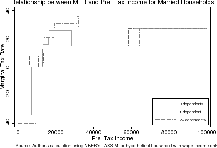
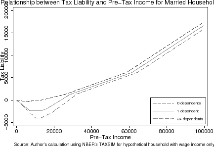
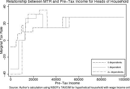
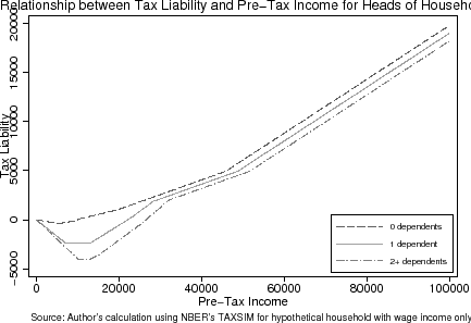
The age-eligibility rules for qualifying a child as a dependent provide an opportunity to, first, consistently estimate a labor supply response to taxation and, second, to assess whether the mechanisms by which households respond are attributable to variation in marginal tax rates. I estimate a labor supply response by exploiting that eligibility for a child primarily hinges on whether s/he is strictly under 19 (or 24 if s/he is a full-time student) as of the end of the calendar year. The benefits of having an eligible dependent are that a household is allowed to exempt more income and to face a tax schedule with, on the whole, lower statutory and effective marginal tax rates due to the Earned Income Tax Credit.⁷ The December 31st cut-off date lends itself nicely to an experiment entailing the quasi-random assignment of households to a particular tax schedule (see Figures (1) and (2)).⁸ Households with a child turning 19 (or 24) on December 31st of a calendar year are not allowed to claim him/her as an eligible dependent whereas those with a child turning 19 on the subsequent January 1st are allowed.⁹

Because only a subset of households experience changes in the marginal tax rate due to a dependent (see Figures (1) and (2)), whereas all households face average tax rate changes, I identify the mechanisms by which fathers and mothers respond to the tax schedule. Observing that households experiencing marginal tax rate changes adjust their labor supply, while the other households do not, means that the lifecycle model is an appropriate approximation of behavior. If, on the other hand, those experiencing only average tax rate changes also respond to the tax schedule, this finding presents a puzzle for the lifecycle model.

The key identifying assumption in the regression discontinuity design is that households with similarly aged children are also similar in many observed and unobserved ways. Most notably, within a narrow range of the December 31st cut-off for having an age-eligible child, households are assumed to be at similar stages of the lifecycle and to have similar levels of lifetime income. This assumption allows for a causal estimate of the effect of the age-eligibility rule on labor supply. An attractive feature of the regression discontinuity design is that, like in a randomized controlled trial, this identifying assumption is testable (Lee, 2005). The identification strategy also entails households' knowing when their children turn 19 (or 24) and being aware that they can no longer claim their dependent. In this sense, the changes in the tax schedule that households experience upon losing an age-eligible dependent are fully anticipated. A final advantage of the regression discontinuity design is that I am able to isolate exogenous marginal and average tax changes that households near the cut-off would experience if they were to lose or gain an eligible dependent. By doing so, I can whether solely marginal tax incentives provide intertemporal labor supply incentives.

Estimating the Labor Supply Effect of the Age-Eligibility Rule

Consider a unitary decision-making household that has one child, and suppose its labor supply in period ( $Y_{it}$ ) can be expressed as the following structural equation:

$\begin{displaymath} Y_{it} = \beta_0 + \theta T_{it} + g(a_{c}) + X_i\beta + \epsilon _{it} \end{displaymath}$

(4)

where $\beta_0$ is an intercept term, $\beta$ is a vector of coefficients, and $g(\cdot)$ is an arbitrarily non-linear, smooth, continuous function of the age of household

's child. $T_{it}$ is an indicator for whether household

faces a tax schedule with an age-eligible dependent.¹⁰ The vector

contains observable (predetermined) characteristics of household

, and $\epsilon_{it}$ is an unobservable determinant of labor supply that is possibly correlated with

. In equation (4), $\theta$ is the effect of claiming a dependent on labor supply, which coincides with facing a lower tax liability and a different set of statutory and effective marginal tax rates.

Other equations of interest include the first-stage and reduced-form equations:

$\displaystyle T_{it}$	$\textstyle =$	$\displaystyle \gamma_0 + \delta_{i} A^{19}_{i}(a_{c}) + h(a_{c}) + X_i\gamma + \nu _{it}$	(5)
$\displaystyle Y_{it}$	$\textstyle =$	$\displaystyle \pi_0 + \pi_{1i} A^{19}_i(a_{c}) + k(a_{c}) + X_i\pi + \psi_{it}.$	(6)

$A^{19}_{i}$ is an indicator for whether household

's child is 19 years old or older. Similar to the structural equation, $\gamma_0$ and $\pi_0$ are intercept terms, while $\beta$ and $\pi$ are vectors of coefficients. Like $g(\cdot)$ , $h(\cdot)$ and $k(\cdot)$ are arbitrarily non-linear, smooth, continuous functions of the age of the child,

. $\nu_{it}$ is an unobserved determinant of $T_{it}$ , and it is possibly correlated with $A^{19}_i(a_c)$ . The parameter $\delta_{i}$ in the first-stage equation represents the effects of the the age-eligibility rule on whether a household claims a dependent. It is allowed to vary across households because the age-eligibility rule may not affect all households equally due to the other (less influential) eligibility tests. The reduced-form parameter $\pi_{1i} = \theta \delta_{i}$ is the effect of the age-eligibility rule on household labor supply. It is larger when the effect of the age-eligibility rule on whether the household claims a dependent is large.

Identification of all the parameters in (4) to (6) rests on four conditions (McCrary and Royer, 2005; Hahn, Todd, and van der Klauuw, 2001; Lee, 2003). First, the household's labor supply as a function of the child's age must be smooth in the absence of the age-eligibility rules. Second, households around the age-eligibility cut-offs must be exchangeable so that barely ineligible households are an appropriate counterfactual for barely eligible households. Third, there must be a discontinuity in the treatment assignment mechanism, and age-eligibility rules must influence whether households claim an age-eligible dependent on their tax returns. Fourth, the age-eligibility rule can only influence households' treatment in a monotone way. Taken together, the first three conditions ensure that the estimated effect of the age-eligibility rule on household labor supply does not capture extraneous effects, such as those of households' levels of lifetime wealth or preferences for leisure. The fourth condition allows for a local average treatment effect (LATE) interpretation of $\theta$ (Imbens and Angrist, 1994).

An attractive feature of the regression discontinuity design is that these conditions also correspond to a large number of testable predictions, which can increase the confidence that the estimates are valid. In the next section, I present evidence that, based on implications of the first three conditions, there is not sufficient evidence to reject the validity of the research design. There may, however, be a concern that the monotonicity condition may not be met. Thus far, I have defined the "treatment" facing a different tax schedule due to having an eligible dependent. In this case, the monotonicity assumption is trivially satisfied in that an age-eligible dependent corresponds to a different tax schedule and lowers tax liabilities for all households. For a treatment defined in terms of changes in the marginal tax rate, which is useful for computing labor supply elasticities, due to the non-increasing structure of marginal tax rates as a function of taxable income, the monotonicity assumption may not hold (see Figures (1) and (2)). That is, it is possible for the age-eligibility rule to both increase and decrease a household's marginal tax rate, depending on the household's characteristics. In the next subsection, I discuss in further detail the mechanisms for the effect of the age-eligibility rule in light of its non-monotonic effect on the marginal tax rate. Also, when interpreting the results from estimation, I discuss the difficulty of interpreting $\theta$ as a LATE parameter.

To see the basis of the identification strategy more formally, consider households with a child over 19 by an amount $\Delta$ ( $a_{c} = 19 + \Delta$ ), who are ineligible to claim a dependent, and households with a child under 19 ( $a_{c} = 19 - \Delta$ ), who are eligible. In general, it is likely that for large values of $\Delta$ , $\epsilon_{it}$ (and therefore $\psi_{it}$ ) is correlated with having an age-eligible dependent, the household's tax schedule, and labor supply.¹¹ As such, the simplest comparison of comparing the labor supply behavior of all households with and without an age-eligible dependent fails to produce a consistent estimate of $\pi_{1}$ . The Appendix describes why this comparison is invalid in greater algebraic detail.

To consistently estimate $\pi_{1}$ , consider a sequence of estimators for different values of $\Delta$ . As $\Delta$ becomes smaller, the two types of families become increasingly comparable in all ways, except in whether they can claim a dependent. In the limit as $\Delta \rightarrow 0$ , the average observables for the two types of families are the same:

$\displaystyle \lim_{\Delta \rightarrow 0} E[k(a_{c}) \vert a_c=19 + \Delta]$	$\textstyle =$	$\displaystyle \lim_{\Delta \rightarrow 0} E[k(a_{c}) \vert a_c=19 - \Delta]$
$\displaystyle \lim_{\Delta \rightarrow 0} E[X_i\vert a_c=19 + \Delta ]$	$\textstyle =$	$\displaystyle \lim_{\Delta \rightarrow 0} E[X_i\vert a_c=19 - \Delta].$

The unobservables are the same as well:

$\displaystyle \lim_{\Delta \rightarrow 0} E[\psi_{it}\vert a_c=19 + \Delta ]$	$\textstyle =$	$\displaystyle \lim_{\Delta \rightarrow 0} E[\psi_{it}\vert a_c=19 - \Delta ].$

A comparison of barely eligible and barely ineligible households allows for a consistent estimate of the reduced-form parameter:

$\begin{displaymath} \pi_{1i} = \lim_{\Delta \rightarrow 0} E[Y_i\vert a_c=19 + \Delta] - \lim_{\Delta \rightarrow 0} E[Y_i\vert a_c=19 - \Delta]. \end{displaymath}$

(7)

A similar argument can be made for identifying $\delta$ in the first-stage equation. Though it is impossible to be certain that households are similar in unobservable dimensions, for any specific small value of $\Delta$ , one can compare any baseline or pre-existing characteristic of the two types of households, and reject the research design if the households near the age-eligibility cut-off differ systematically.

To estimate the the parameters of this model, it is helpful to graph the outcome of interest against the age of the child to, first, visually detect the effect of the age-eligibility rule, and to, second, estimate the magnitudes of $\pi_{1i}$ and $\delta_i$ . In the data, which I further discuss in the next section, age is measured in months and is therefore "binned" and not continuous. To estimate the reduced-form effects of the age-eligibility rule, I plot the age-specific averages of fathers' and mothers' labor supply, and fit a flexible global polynomial through the age-specific averages (DiNardo and Lee, 2004; Lee and Card, 2004). Fitting a global polynomial entails making a parametric assumption about the underlying function, so in discussing the results, I present alternative fits as a robustness check. If there is an effect of the age-eligibility rule on fathers' or mothers' labor supply, the polynomial ought to detect a break in the age-specific averages around the age-eligibility cut-offs. The discontinuity in the age-specific averages around the age-eligibility thresholds ought to be graphically visible as well. The magnitude of this break represents the effect of the age-eligibility rule.

To estimate the magnitude of this break, I fit third-order global polynomials through the age-specific local averages of fathers' and mothers' labor supply, allowing the slope and intercept to vary according to whether the child's age is under 19, between 19 and 24, or 24 and older. I also fit first- and second-order polynomials through the local averages to show the sensitivity of the estimated break to assumptions about functional form. I normalize the age of the child to equal zero at ages 19 and 24 in order to readily compute the reduced form parameters, $\lim_{\Delta \rightarrow 0} E[Y_i\vert a_c=19 + \Delta] - \lim_{\Delta \rightarrow 0} E[Y_i\vert a_c=19 - \Delta]$ and $\lim_{\Delta \rightarrow 0} E[Y_i\vert a_c=24 + \Delta] - \lim_{\Delta \rightarrow 0} E[Y_i\vert a_c=24 - \Delta]$ , at each age-eligibility cut-off. Dropping the subscripts, I estimate the following equations through the local averages:

$\displaystyle Y$	$\textstyle =$	$\displaystyle \pi_{1}^{19}A^{19} + \alpha_{1} A^{24} + \phi_{0}(P)A + \phi_{1}(P)A^{19}A + \phi_{2}(P)A^{24}A + \xi$	(8)
$\displaystyle Y$	$\textstyle =$	$\displaystyle \pi_{1}^{24}A^{24} + \alpha_{2} A^{24} + \phi_{0}(P)\tilde{A} + \phi_{1}(P)A^{19}\tilde{A} + \phi_{2}(P)A^{24}\tilde{A} + \xi,$

where $A^{j}$ is an indicator for whether the child is older than

years ( $j \in \{19,24\}$ ),

and $\tilde{A}$ are the normalized ages of the child, and $\phi_{k}(P)$ is a low-order polynomial in

.¹² The estimated parameters $\hat{\pi}_{1}^{19}$ and $\hat{\pi}_{1}^{24}$ give us the reduced-form parameters of interest. In theory and practice, the fitted line should go through the local averages. The standard error of the magnitude of the discontinuity in the polynomial at the age-eligibility cut-offs is clustered on age, since the variation in the circles is driven by 480 local averages.

Estimating the Mechanisms for the Labor Supply Effect of the Age-Eligibility Rule

To understand whether the variation in marginal tax rates of barely eligible and ineligible households drives their labor supply responses to the age-eligibility rule, I adapt a "simulated instrument" to the regression discontinuity framework (Rothstein, 2007; Leigh, 2004; Dahl and Lochner, 2005). All tax rates and liabilities depend on taxable income, which in turn depends on a household's deductions, exemptions, and pre-tax income. Furthermore, tax rates affect pre-tax income via labor supply and other incentives. Using demographic variables to predict pre-tax income breaks the simultaneity with tax rates, and using this predicted measure of pre-tax income allows for estimates of marginal and average tax rates, as well as liabilities, that are independent of (unobserved) labor supply effort.

Mechanically, it is possible to fit polynomials through age-specific averages of these instrumented marginal tax rates in order to obtain an estimate of $\delta_{i}$ in equation (5). This simply entails combining a household's predicted pre-tax income and their deductions and exemptions to compute their tax rates and liability. As discussed earlier, however, because the age-eligibility rule has a non-monotonic effect on marginal tax rates, this estimate does not yield the structural estimate of the effect of marginal tax rates on households' labor supply (Hahn, Todd, and van der Klauuw, 2001). Furthermore, the elasticity implied by dividing the reduced form parameter by the first-stage parameter, $\delta_i$ , is neither consistent nor a LATE estimate.

Combining the instrumented tax variables with the age-eligibility rule allows for the identification of households who are at "kink" points in the tax schedule. For age-eligible households, it is possible to compute $\hat{\tau}^{+}_{i}$ , which denotes a vector of tax variables corresponding to their tax rates and liabilities taking into account their age-eligible dependents. It is also possible to construct $\hat{\tau}^{-}_{i}$ for these households, which denotes their tax rates and liabilities if they were to lose an age-eligible dependent. When $\hat{\tau}^{+}_{i} \neq \hat{\tau}^{-}_{i}$ , household is at a "kink" point. Age-ineligible households also have analogously defined tax vectors.¹³ Here, an example helps clarify the purpose of these tax vectors and their components. Among age-eligible households $\Delta \tau_{MTR} = \hat{\tau}_{MTR}^{-} - \hat{\tau}_{MTR}^{+} = 10$ means that they are at "kink" in the marginal tax rate schedule such that if they were to lose a dependent, their marginal tax rate would rise by 10 percentage points. The counterfactual for these households are the barely ineligible households who would experience a decrease in their marginal tax rate by 10 percentage points if they were to gain an eligible dependent.

Near the eligibility thresholds, age-ineligible households whose "kink" size equals $\hat{\tau}^{-}_{i} - \hat{\tau}^{+}_{i}$ are thus a counterfactual for age-eligible households whose "kink" size equals $\hat{\tau}^{+}_{i} - \hat{\tau}^{-}_{i}$ . Defining $\Delta \tau$ accordingly for eligible and ineligible households, I augment (8) to:¹⁴

$\displaystyle Y$	$\textstyle =$	$\displaystyle \pi_{1}^{19}A^{19} + \pi_{1}^{24}A^{24} + \phi_{0}(P)A + \phi_{1}(P)A^{19}A + \phi_{2}(P)A^{24}A + \gamma \Delta \tau + \gamma^{19}A^{19} \Delta \tau +$	(9)
		$\displaystyle \gamma^{24}A^{24} \Delta \tau + \xi.$

The vectors $\gamma^{19}$ and $\gamma^{24}$ contain the coefficients on the interaction between the age-eligibility rule and the three tax variables. The coefficient for the interaction between the age-eligibility rule and the magnitude of the marginal tax rate "kink" is $\gamma^{j}_{MTR}$ . Similarly, $\gamma^{j}_{ATR}$ and $\gamma^{j}_{TL}$ denote the coefficients on the interactions with the average tax rate and tax liability "kinks."¹⁵

According to the lifecycle model, $\pi_{1}^{19} = \pi_{1}^{24} = 0$ , and the age-eligibility rule does not have an independent effect on fathers' and mothers' labor supply. Instead, the age-eligibility rule affects labor supply through the disincentives of higher marginal tax rates. If it is indeed the case that higher marginal tax rates cause work disincentives, then $\gamma^{j}_{MTR}$ should be negative. In other words, the age-eligibility rule should only matter to the extent that it coincides with changes in the marginal tax rate. Also, in a lifecycle model, the coefficients on the interactions of $A^{j}$ and the average tax rate ( $\gamma^{j}_{ATR}$ ) and tax liability ( $\gamma^{j}_{TL}$ ) "kinks" should be zero under the null hypothesis of lifecycle behavior.

If, on the other hand, the lifecycle model is not a good approximation of behavior, it is possible to observe the age-eligibility rule having an independent effect on labor supply or the age-eligibility rule affecting labor supply decisions through average tax rates. Finding that the coefficient on the interaction of $A^{j}$ and the average tax rate is negative ( $\gamma^{j}_{ATR}$ ) would be consistent with the "schmeduling" hypothesis of decision-making (Liebman and Zeckhauser, 2004). If households are myopic and a static labor supply model characterizes their behavior, the substitution effect in static labor supply model suggests that $\gamma^{j}_{MTR} < 0$ while $\gamma^{j}_{TL} > 0$ is consistent with a negative income effect.

Sample Selection and Household Formation

Thus far, I have assumed that it is possible to randomly sample from households near the age-eligibility rules. This is a sufficient condition for being able to consistently estimate the reduced form and structural estimates of the effect of facing a different tax schedule on household labor supply. It is, however, possible for the age-dependent exemption to affect household formation. That is, children may delay leaving their parents, as well as other transitions to adulthood, in which case households observed around the age-eligibility cut-offs comprise self-selected groups.

Empirically, one can assess the sample selection problem by estimating the effect of the age-eligibility rules on the probability of being observed.¹⁶ Alternatively, testing for discontinuities in the distribution of the running variable provides evidence on the extent to which sample selection is an issue (McCrary, 2004). In either case, if the estimated effect is zero, it may be possible to consistently estimate the reduced form and structural parameters. If this effect is not zero, the resulting estimates of the reduced form and structural parameters are an admixture of the treatment effect and a selection effect. It is not possible to consistently estimate the parameters of the model, however one may be able to generate consistent bounds on this effect (Lee, 2003).

5 Data

The data for this paper are from the 1990-1993, 1996, and 2001 panels of the Survey of Income and Program Particiapation (SIPP). These nationally representative panels of households span the calendar years 1990-1994, 1996, 1997, 1998, 2001, and 2002. Unlike the public-use versions of the Census or the Current Population Survey (CPS), the SIPP variables include the month of an individual's birth rather than just the year, quarter, or age at last birthday. This means that there is greater flexibility than otherwise to finely separate the older 18-year-olds from their younger counterparts, and similarly the younger 19-year-olds from the older ones. This is an advantage of the SIPP to the extent that there is seasonality in births that would be more pronounced with less precise data on births (such as with quarters) (Bound, Jaeger, and Baker, 1995). In addition, the identification strategy requires observable and unobservable similarity among households around the December 31st cut-off, and this condition is more likely to hold in a narrower range of dates.

Each observation in the dataset is a "child" sampled in the SIPP, where the term "child" means those who can be linked to a parent. I further limit this set to children under 40 living at home with a parent during part or all of a calendar year, which yields 373,966 child-parent observations. Low socio-economic status households are oversampled in the SIPP, and though the Census Bureau provides sampling weights, all estimates in this paper are unweighted.¹⁷ A set of descriptive characteristics for the sample as a whole are in Table (1). The sample is 67% white, and parents, on average, have 12 years of education. Fifty-three percent of children under 40 are from two-parent households. The columns of Table (1) suggest that there are statistically significant differences in the parental characteristics of households with older (ineligible) and younger (eligible) children. For example, older children are less likely to be a part of a two-parent household and more likely to have less educated parents. These differences lend support for the necessity of a research design that addresses this heterogeneity.

Data for marginal and average tax rates, as well as liabilities, are from the NBER's tax simulator (TAXSIM) program (Feenberg, October 7, 2005; Feenberg and Coutts, 1993). For each child-parent observation, TAXSIM computes marginal and average tax rates using the parents' marital status, the number of eligible dependents, and predicted measures of pre-tax earnings, interest income, and other income items appearing on the IRS Form 1040. Constructing the counterfactual tax changes entails the same TAXSIM calculation but instead using the counterfactual number of dependents. Because the core waves of the SIPP do not report charitable and other itemized deductions, I assume that all households are non-itemizers in executing the TAXSIM calculations.¹⁸

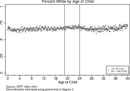
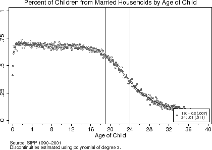
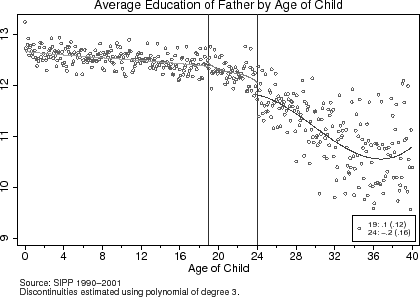
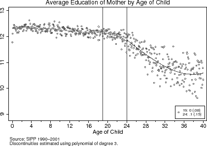
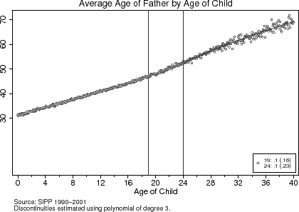
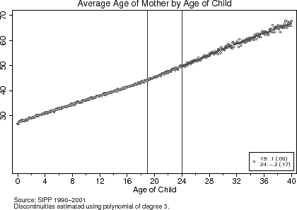
To test the validity of the research design, I present a set of baseline characteristics of the parents around the age-eligibility cut-offs in Table (2). The third and fifth columns report the estimated differences in these characteristics at the age-19 and age-24 eligibility cut-offs, respectively. The same characteristics are graphically represented in Figures (4) to (6). The results from Table (2) and these figures suggest that around the age 19 and age 24 age-eligibility cut-offs, parents are equally likely to be white, while the average education levels and ages of the fathers and mothers are also similar around the cut-offs. Though these findings do not prove that the unobservable characteristics of households are the same around the age-eligibility cut-offs, they do not provide any a priori grounds for rejecting the research design.

6 Results

In this section, I discuss the effect of the age-eligibility rule on a child's eligibility status, and present the reduced form results on the effect of the age-eligibility rule on households' labor supply outcomes. In the next section, I interpret these results in light of the structural equation in (4). The labor supply outcomes analyzed include fathers' and mothers' annual hours of work, as well as the corresponding employment participation rates. I examine these measures of labor supply, rather than labor earnings, in order to isolate a real behavioral response, rather than one related to income reporting or income shifting (Slemrod, 1990).

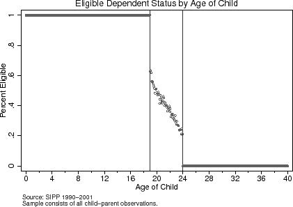
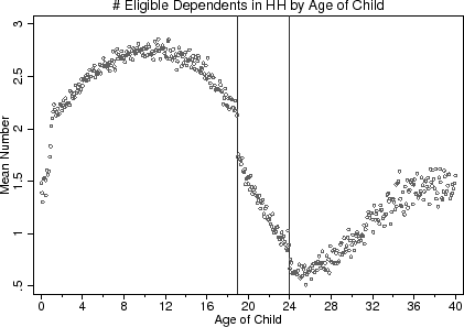
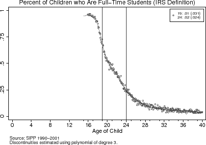
At the age-19 and age-24 cut-offs in Figure (3), the age-eligibility rule has a noticeable effect on whether a household is eligible to claim a child as a dependent. The top panel shows that the likelihood that an 18-year-old child is eligible is 1 while this probability drops to around 0.6 for 19-year-old children. In determining eligibility, I assume that the other eligibility tests, such as the support test, do not apply.¹⁹ This probability does not drop to zero at the age-19 threshold because parents can claim a child if they are a full-time student, and in the SIPP sample, around 60% of 19-year-old children are full-time students. The bottom panel of Figure (3) shows how the total number of eligible dependents in a child's household is discontinuous at ages 19 and 24. Based on the discontinuities observed in Figure (3), the age-eligibility rule provides variation in the tax schedule that households face around the age-19 and age-24 cut-offs.²⁰

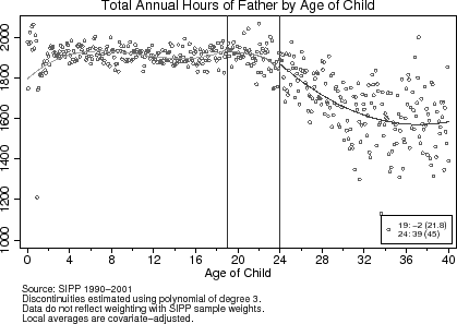
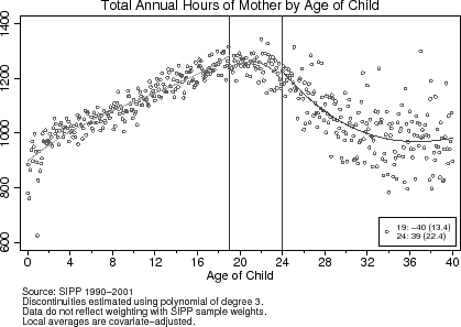
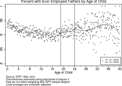
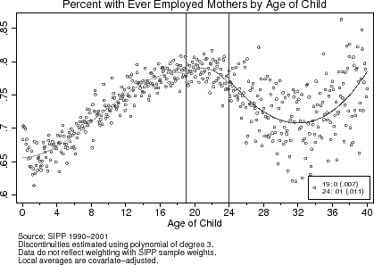
Estimates of the reduced-form effects of the age-eligibility rules are in table (3). Here, I present estimates of $\pi_{1i}$ in equation (7), which I estimate by fitting first-, second-, and third-order polynomials through the covariate unadjusted and adjusted local averages. Figures (7) and (8) display the covariate-adjusted local averages for annual hours and participation among fathers and mothers.

In Figure (7), the curvature in the local averages leads one to reject the linear specification for the conditional expectations function. For fathers' annual hours, the sizeable estimate given by the quadratic specification belies the visual smoothness of the local averages, particularly around the age-19 cutoff. The third-order polynomial, plotted in the figure, appears to best approximate the conditional expectations formulate for the effect of the age-eligibility rule.

Across all three polynomial approximations, the age-eligibility rule results in fewer annual hours among mothers at the age-19 cutoff. The third-order polynomial suggests that the estimated effect of having an eligible dependent is to increase annual labor supply by 40 hours. Alternatively, mothers are likely to work 40 hours less upon losing the age exemption. The result for mothers around the age-24 cut-off deserves a more careful interpretation. First, the amount of variability in this region is significantly greater than elsewhere. This is due to the fact that there are not many "older" children living with their parents, and the ones who do are likely to differ from households with similarly aged parents but without "children" living at home. Second, as I discuss in greater detail in the next section, the magnitude and direction of the induced marginal tax rate changes is different at the age-24 cutoff than at the age-19 one.

For both fathers and mothers, the age-eligibility rule has little to no effect on the participation decision. This result is not surprising for fathers, who work, on average, over 1,800 hours per year (see Table (1)) and among whom there is no effect of the age-eligibility rule on annual hours. The result for mothers differs from the previous literature's finding that women's labor supply responses to taxation are larger on the extensive margin than on the intensive margin (Meyer and Rosenbaum, 2001; Eissa and Liebman, 1996). Mothers' non-response in participation, however, is consistent with the lifecycle model. In contrast to previous studies that exploit unanticipated tax policy changes as a source of variation in tax rates, the tax changes induced by the age-eligibility rule are are anticipated and do not correspond to revisions to lifetime wealth. Furthermore, with the regression discontinuity design, I arguably compare households with similar lifetime wealth and unobserved preferences for non-market time, which are determinants of the participation decision. These two explanations may account for the relatively larger intensive margin response among mothers.

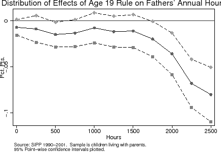
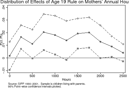
To deconstruct the intensive labor supply response, I uncover where in the distribution of hours the age-eligibility rule has the largest effect by estimating the following sequence of regressions for annual hours worked ():

$\begin{displaymath} 1(Y \leq y) = \pi_{1,y}^{19}A^{19} + \alpha A^{24} + \phi_{0,y}(P)A + \phi_{1,y}(P)A^{19}A + \phi_{2,y}(P)A^{24}A + \xi_{y}, \end{displaymath}$

where $1(Y \leq y)$ is an indicator for whether annual hours is less than an amount

. For each value of

, $\pi_{1,y}^{j}$ indicates the effect of the age-eligibility rule on the likelihood a parent works fewer than

hours. Larger values of $\pi_{1,y}^{j}$ indicate a larger effect of the age-eligibility rule at

annual hours of work (Angrist and Imbens, 1995; McCrary and Royer, 2005). Figure (9) plots the estimates for $\pi_{1,y}^{19}$ corresponding to different levels of hours for fathers and mothers. The shape of the distribution for fathers suggests that the effect of there is no effect of the age-eligibility rule for the majority of fathers (i.e. those working fewer than 2,000 hours per year). Among fathers working 2,000 hours or more, barely ineligible fathers work more hours. The distribution of effects for mothers suggests that those working part-time and nearly full-time are the ones most affected by the age-eligibility rules, and that they are the ones most likely to decrease their hours of work upon losing an age-eligible dependent.

7 Interpretation

In this section, I interpret the findings above in the context of a standard lifecycle labor supply model in order to assess the magnitude of households' (particularly mothers') labor supply responses, and to infer households' intertemporal labor supply elasticities. Recall that barely ineligible households are a counterfactual for barely eligible households in the subsequent year. I first discuss a LATE interpretation of the labor supply response to the age-eligibility rule. This interpretation points in the direction of sizeable (and implausible) intertemporal labor supply elasticity estimates for mothers. The estimates for fathers are statistically insignificant from zero, but the point estimates are well within the range of previous estimates. I then provide an alternative explanation of the labor supply response, and present evidence suggesting that the dominant mechanism for the labor supply response may not be through marginal tax rates. Overall, I argue that the effect of losing an age-eligible dependent appears not to work through the concomitant changes in the marginal tax rate, which suggests that it may be tenuous to assume that predictable changes in income have no effect on labor supply (holding after-tax wages constant).

Effect of Age-Eligibility Rule on Tax Rates and Liabilities

Quantifying how tax rates change when households lose dependents is necessary to know the incentives they face. With an age-eligible dependent, households face a different tax schedule than otherwise that enables them to exempt more income and face a different set of statutory and effective marginal tax rates. As discussed earlier, Figures (1) and (2) illustrate how the presence of dependents changes the relationships among marginal tax rates, tax liabilities, and pre-tax income for married and heads of households, respectively. The presence of an age-eligible dependent lowers tax liabilities at all levels of income. The effect of an age-eligible dependent on a household's marginal tax rate, however, is less clear. At high and very low levels of income, having a dependent lowers a household's marginal tax rate whereas between $20,000 and $40,000 (in 2001 $ for married households) of pre-tax income, marginal tax rates are higher with an age-eligible dependent. For some ranges of income, an age-eligible dependent does not change a household's marginal tax rate.

As discussed earlier, estimating how the age-eligibility rule affects a household's marginal tax rates presents a challenge because the latter is a non-linear and non-monotonic function of taxable income. In turn, taxable income depends on the household's deductions as well as the behavioral response to being (in)eligible for the dependent exemption and the EITC (Triest, 1998). To address this simultaneity between a household's taxable income and its exemptions, I construct a "simulated instrument." I use all child-parent observations to run a Tobit regression of pre-tax income on a vector of pre-determined characteristics.²¹ I then predict pre-tax income. With this prediction and using households' actual dependent-eligibility status, I use the NBER's TAXSIM program to produce a set of predicted tax variables for each child-parent observation in the data.

Table (4) presents the results from constructing a "simulated instrument" and fitting a third-order global polynomial (see Equation (8)) through the local averages of the tax variables (analogous to Table (3)). According to this table, the effects of the age-eligibility rule on tax rates and liabilities differ depending on whether one is looking at the age-19 or age-24 cutoffs. This is largely due to the fact that the distribution of households' pre-determined characteristics are correlated with the age of the child over large age ranges. In addition, the non-linearities in the tax schedule (seen in Figures (1) and (2), mean that the direction of the age-eligibility rule's effect depends on the distribution of pre-determined characteristics. At the age-19 threshold, I estimate that barely ineligible households face a net-of-tax rate that is 0.5 percentage points (or 0.3%) lower than their barely eligible counterparts. Barely ineligible households with a 24-year-old child face a net-of-tax rate that is 0.4 percentage points (or 0.6%) higher than those barely eligible.

While neither of the net-of-tax rate estimates at the age-19 threshold is statistically significant from zero, we can nonetheless discuss the implied labor supply elasticities. The point estimates imply a labor supply elasticity of around 0.4 for fathers but an implausibly large elasticity of about 12 for mothers.²² This estimate for mothers vastly exceeds the usual estimates found for women in the literature, which suggest an intertemporal elasticity of no larger than one. Because the age-eligibility rule can both increase or decrease a household's marginal tax rate, the estimated intertemporal elastiticities for mothers and fathers cannot have a typical LATE interpretation. It is, however, possible to sign the bias in the estimated effect from the true LATE parameter. Assuming that the the response in hours due to changes in the marginal tax rate are in the direction predicted by the lifecycle model, these estimates are a lower bound on the true parameters.²³

In the context of the age-eligibility rule affecting the entire tax schedule or the tax liability that a household faces, the subpopulation likely to be affected is relatively broad in this case, and captures the majority of households.²⁴ Hence the monotonicity assumption that is needed for a LATE interpretation is unlikely to be violated. Indeed, as the bottom half of Table (4) shows, the age-eligibility rule increases the average tax rate by about 1 percentage point (or 4.3%) among those near the age-19 cutoff. The corresponding increase in households' tax liabilities is $430. The results are in the same direction but somewhat more muted at the age-24 cutoff as the number of households affected is considerably less.²⁵

Mechanisms for the Labor Supply Response to the Age-Eligibility Rule

It is possible to identify whether marginal tax rates or average tax rates (or neither) comprise the mechanism through which age-ineligible households are incentivized to decrease their labor supply. For each child-parent observation, I construct a set of counterfactual tax variables. For barely eligible households, I use TAXSIM to to compute their tax rates and liability if they were to become ineligible. Similarly, TAXSIM produces a set of tax variables for barely ineligible households. Table (5) shows that around 30% of those around the age-19 cutoff, and 40% of those around the age-24 cutoff, would experience a change in their marginal (and hence their net-of-) tax rate if they were to lose or gain a dependent. According to this exercise, virtually all households would experience a change in their average rate and their tax liability upon losing or gaining a dependent.

Another goal of this particular TAXSIM exercise is to identify households who are at similarly sized kinks on both sides of the age-eligibility rule. In Table(5), around 30% of households around the age-19 cut-off, and 40% around the age-24 cut-off, would experience changes in their marginal tax rates if they were to lose or gain an eligible dependent. Table (5) also reports the average magnitude of the tax changes that households would experience if they were to gain or lose a dependent. Around the age-19 cut-off, the average increase is about half a percentage point whereas around the age-24 cut-off, households' marginal tax rates would decrease by 2.5 percentage points if they were to lose a dependent.²⁶ This identification enables a test of the lifecycle prediction that the age-eligibility rule alters labor supply incentives through the net-of-tax rate if the effect of the age-eligibility rule is identified among those who would experience changes in their marginal tax rates. In addition, households who are not at a net-of-tax rate "kink" should not be affected by the age-eligibility rule, according to the lifecycle hypothesis.

Table (6) presents the results from estimating (9). In Columns (1) and (3), I only interact the magnitude of the marginal tax rate "kink" with the age-eligibility rule whereas in Columns (2) and (4), I also include interactions with the average tax rate "kink." From this table, at best, the variation in marginal tax rates can only partially account for the labor supply response of fathers and mothers. Barely eligible fathers facing higher marginal tax rates are likely to increase their labor supply upon losing an age-eligible dependent (Columns (1) and (2)), which is at odds with the lifecycle model. In Column (3), barely eligible mothers, on the other hand, adjust their labor supply consistent with lifecycle labor supply behavior, and are likely to reduce their annual hours when faced with higher marginal tax rates around the age-19 cut-off. The statistically significant coefficient on the age-19 dummy in Column (3) suggests that the age-eligibility rule has an independent effect on mothers' labor supply. Indeed, when controlling for the average tax rate changes facing households in Column (4), the independent effect of the age-eligibility rule disappears. And not only does the direction of the effect of the marginal tax rate incentives reverse itself for mothers in Column (4), differences in the average tax rate between barely eligible and ineligible households explain the negative effect of the age-eligibility rule, consistent with the "schmeduling" hypothesis.

Robustness Check

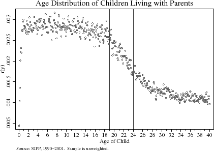
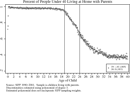
As alluded to earlier, a key issue for identifying the effect of the age-eligibility rule is whether the sample of child-parent observations around the age-19 and age-24 thresholds comprise self-selected groups. Non-random selection around each side of the age-eligibility cut-offs can occur if children delay leaving their parents' home or if, around the time of birth, households manipulate the timing of their children's births (Chandra and Dickert-Conlin, 1999). To obviate the concern that the sample of children living with their parents is a self-selected group around the age-eligibility cut-offs, I present the age distribution of this sample in Figure (11). If there were selection into the sample and the probability of being observed were different on each side of the age-eligibility rule, one would expect to see a break in the age density at the thresholds. Using the methods in McCrary (2004), I cannot reject that the distribution is continuous at ages 19 and 24.²⁷ Hence I am reasonably confident that mothers' labor supply responses to the age-eligibility rule are not instead due to issues concerning household formation.

Another potential concern about the effect of the age-eligibility rule, particularly for mothers, is that the result is a false-positive. If the location of the discontinuity were instead elsewhere and not at the December/January cut-off, it may be possible that the polynomial would detect a discontinuity at the age-19 threshold when in fact the "true" experiment is either earlier or later in the calendar year. Table (7) presents estimates of the effect of the age-eligibility rule at various cut-offs. In column (2), I shift the "experiment" to the July when the child is 18 by redefining the age-19 dummy in (8) to equal 1 for children aged 18 and 1/2 or older. Similarly in column (3), the "experiment" occurs in the July when the child is 19. In both cases, the effect of the age-eligibility rule for mothers decreases (in absolute value) and becomes statistically insignificant. For mothers, the standard errors are also somewhat higher in columns (2) and (3) than in column (1), which re-presents the relevant estimates from Table (3). Because the estimates in columns (2) and (3) are not statistically different from those in column (1), these placebo tests merely suggest that the experiment is not occurring at another point in time.

8 Conclusions and Policy Implications

The effect of an anticipated increase in a household's tax liability on a household's labor supply is difficult to reconcile with the predictions of a lifecycle labor supply model. Though it is difficult to detect a response among fathers, mothers supply about 40 fewer hours per year upon losing an age-eligible dependent. They are equally likely to participate in the labor market as their barely eligible counterparts. Though the implied intertemporal labor supply elasticity estimates for mothers is 12, this estimate is implausibly large and further analysis shows that average tax rates have an independent effect, controlling for the accompanying changes in households' marginal tax rates. This finding presents a puzzle for the standard lifecycle labor supply model, which predicts that anticipated changes in income do not influence the household-specific lifecycle variation in hours.²⁸

Though it seems that the behavior of households is inconsistent with the predictions of a lifecycle model, there are nonetheless important lessons from the results of the quasi-experiment studied. First, the tax system, through policies like the dependent exemption and the EITC, can encourage households' labor supply decisions, even if this process occurs through a mechanism that economists have yet to precisely identify. This finding is particularly important in light of the federal government's increasing reliance on the tax system to achieve its redistributional goals. Second, for mothers, the effects of these policies is largest for part-time and full-time workers than it is for those entering the labor market. This suggests that intertemporal tax incentives are not as effective at inducing non-working mothers into the labor market as they are at encouraging working mothers to work longer hours.

Bibliography

ANGRIST, J. D., AND G. W. IMBENS (1995): "Two-Stage Least Squares Estimation of Average Causal Effects in Models with Variable Treatment Intensity," Journal of the American Statistical Association, 90(430), 431-442.

AUERBACH, A., AND J. SLEMROD (1997):

"The Economic Effects of TRA86," Journal of Economic Literature, 35(2), 589-632.

BLUNDELL, R., AND T. MACURDY (1999):

"Labor Supply: A Review of Alternative Approaches," in The Handbook of Labor Economics, Volume 3A, ed. by O. Ashenfelter, and D. E. Card. Elsevier, Amsterdam.

BOUND, J., D. JAEGER, AND R. BAKER (1995):

"Problems with Instrumental Variables Estimation When the Correlation between the Instruments and the Endogenous Explanatory Variable Is Weak," Journal of the American Statistical Association, 90, 443-450.

BURTLESS, G., AND J. HAUSMAN (1978):

"The Effect of Taxation on Labor Supply: Evaluating the Gary Income Maintenance Experiment," Journal of Political Economy, 86, 1101-1130.

CAMPBELL, J., AND N. G. MANKIW (1987):

"Permanent and Transitory Components in Macroeconomic Fluctuations," NBER Working Paper No. 2167.

CARD, D. E. (1990):

"Intertemporal Labor Supply: An Assessment," NBER Working Paper #3602.

CARROLL, C. D., R. E. HALL, AND S. P. ZELDES (1992):

"The Buffer-Stock Theory of Saving: Some Microeconomic Evidence," Brookings Papers on Economic Activity, 1992(2), 61-156.

CHANDRA, A., AND S. DICKERT-CONLIN (1999):

"Taxes and the Timing of Birth," Journal of Political Economy, 107, 161-177.

COURANT, P. N., E. GRAMLICH, AND J. LAITNER (1984):

"A Dynamic Micro Estimate of the Life-Cycle Model," in Retirement and Economic Behavior, ed. by H. G. Aaron, and G. Burtless. Brookings Institute, Washington, D.C.

DAHL, G., AND L. LOCHNER (2005):

"The Impact of Family Income on Child Achievement," NBER Working Paper No. 11279.

DAS, M., W. NEWEY, AND F. VELLA (January 2003):

"Nonparametric Estimation of Sample Selection Models," Review of Economic Studies, 70(1), 22-58.

DEATON, A. (1991):

"Saving and Liquidity Constraints," Econometrica, 59, 819-863.

DINARDO, J. E., AND D. S. LEE (2004):

"Economic Impacts of New Unionization on Private Sector Employers: 1984-2001," Quarterly Journal of Economics, 119(4), 1383-1441.

EISSA, N. (1995):

"Taxation and Labor Supply of Married Women: The Tax Reform Act of 1986 As a Natural Experiment," NBER Working Paper #5023.

EISSA, N., AND J. LIEBMAN (1996):

"Labor Supply Response to the Earned Income Tax Credit," Quarterly Journal of Economics, 111(2), 605-637.

FEENBERG, D. (October 7, 2005): "TAXSIM Related Files at the NBER," NBER Website.

FEENBERG, D., AND E. COUTTS (1993):

"An Introduction to the TAXSIM Model," Journal of Policy Analysis and Management, 12(1), 189-194.

FELDMAN, N., AND P. KATUSCAK (2005):

"Should the Average Tax Rate Be Marginalized?," Unpublished manuscript.

FLAVIN, M. A. (1981):

"The Adjustment of Consumption to Changing Expectations about Future Income," Journal of Political Economy, 89(5), 974-1009.

GRUBER, J., AND E. SAEZ (2002):

"Elasticity of Taxable Income: Evidence and Implications," Journal of Public Economics, 84, 1-32.

HAHN, J., P. TODD, AND W. VAN DER KLAUUW (2001):

"Identification and Estimation of Treatment Effects with a Regression-Discontinuity Design," Econometrica, 69(1), 201-209.

HAUSMAN, J., AND J. POTERBA (1987):

"Household Behavior and the Tax Reform Act of 1986," Journal of Economic Perspectives, 1(1), 101-119.

HECKMAN, J. J. (1976):

"The Common Structure of Statistical Models of Truncation, Sample Selection, and Limited Dependent Variations and a Simple Estimator for Such Models," Annals of Economic and Social Measurement, 5, 475-492.

IMBENS, G. W., AND J. D. ANGRIST (1994):

"Identification and Estimation of Local Average Treatment Effects," Econometrica, 62(2), 467-475.

LAIBSON, D. (1997):

"Golden Eggs and Hyperbolic Discounting," Quarterly Journal of Economics, pp. 443-477.

LEE, D. S. (2003):

"Trimming for Bounds on Treatment Effects with Missing Outcomes," Unpublished manuscript.

-------- (2005):

"Randomized Experiments from Non-random Selection in U.S. House Elections," forthcoming in Journal of Econometrics.

LEE, D. S., AND D. E. CARD (2004):

"Regression Discontinuity Inference with Specification Error," University of California, Berkeley, Center for Labor Economics Working Paper #74.

LEIGH, A. (2004):

"Who Benefits from the Earned Income Tax Credit? Incidence Among Recipients, Coworkers, and Firms," Unpublished Manuscript, Australian National University.

LIEBMAN, J., AND R. ZECKHAUSER (2004):

"Schmeduling," Unpublished manuscript.

LOONEY, A., AND M. SINGHAL (2006):

"The Effect of Anticipated Tax Changes on Intertemporal Labor Supply and the Realization of Taxable Income," NBER Working Paper #12417.

MACURDY, T. (1981):

"An Empirical Model of Labor Supply in a Life-Cycle Setting," Journal of Political Economy, 89(6), 1059-1085.

MCCRARY, J. (2004):

"Testing for Manipulation of the Running Variable in the Regression Discontinuity Design," mimeo, University of Michigan.

MCCRARY, J., AND H. ROYER (2005):

"The Effect of Maternal Education on Fertility and Infant Health: Evidence From School Entry Laws Using Exact Date of Birth," mimeo, University of Michigan.

MEYER, B. D., AND D. T. ROSENBAUM (2001):

"Welfare, the Earned Income Tax Credit, and the Labor Supply of Single Mothers," Qarterly Journal of Economics, 116(3), 1063-1114.

MOFFITT, R., AND M. WILHELM (2000):

"Taxation and the Labor Supply Decision of the Affluent," in Does Atlas Shrug? Economic Consequences of Taxing the Rich, ed. by J. Slemrod. Russell Sage Foundation and Harvard University Press.

ROTHSTEIN, J. (2007):

"The Unintended Consequences of Encouraging Work: Is the EITC Good as a NIT?," mimeo, Princeton University.

SAEZ, E. (2003):

"The Effect of Marginal Tax Rates on Income: A Panel Study of Bracket Creep," Journal of Public Economics, 87, 1231-1258.

SHEA, J. (1995):

"Union Contracts and the Life-Cycle/Permanent Income Hypothesis," American Economic Review, 85, 186-200.

SLEMROD, J. (1990):

"Optimal Taxation and Optimal Tax Systems," Journal of Economic Perspectives, 4(1), 157-178.

TRIEST, R. (1998):

"Econometric Issues in Estimating The Behavioral Response to Taxation: A Non-Technical Introduction," National Tax Journal, 1(4).

ZELDES, S. P. (1989):

"Consumption and Liquidity Constraints: An Empirical Investigation," Journal of Political Economy, 97(2), 305-346.

Table 1: Sample Means of Selected Descriptive Characteristics of Parents by Age of Child (Standard Errors in Parentheses, N = 373,966)
	All		19 to	Over 24
Father's Annual Hours	1,818	1,897	1,745	1,161
Father's Annual Hours (standard error)	(2.2)	(2.4)	(6.4)	(8.6)
Mother's Annual Hours	1,078	1,070	1,271	885
Mother's Annual Hours (standard error)	(1.8)	(2.1)	(5.3)	(6.3)
Father's Participation	.926	.944	.916	.769
Father's Participation (standard error)	(.001)	(.001)	(.002)	(.003)
Mother's Participation	.8	.803	.845	.708
Mother's Participation (standard error)	(.001)	(.001)	(.002)	(.003)
Percent White	.667	.662	.686	.671
Percent White (standard error)	(.001)	(.001)	(.002)	(.002)
Father's Education	12.4	12.5	12.3	11.3
Father's Education (standard error)	(.008)	(.008)	(.023)	(.029)
Mother's Education	12.1	12.3	12.1	11.2
Mother's Education (standard error)	(.006)	(.006)	(.018)	(.022)
Father's Age	42	39	49	58
Father's Age (standard error)	(.021)	(.019)	(.042)	(.066)
Mother's Age	39	36	47	56
Mother's Age (standard error)	(.019)	(.016)	(.032)	(.051)
From 2-Parent HH	.525	.672	.492	.161
From 2-Parent HH (standard error)	(.001)	(.001)	(.002)	(.001)
Percent of observations from: 1990	.07	.074	.077	.056
Percent of observations from: 1990 (standard error)	(0)	(.001)	(.001)	(.001)
Percent of observations from: 1991	.113	.119	.122	.092
Percent of observations from: 1991 (standard error)	(.001)	(.001)	(.001)	(.001)
Percent of observations from: 1992	.103	.11	.109	.08
Percent of observations from: 1992 (standard error)	(0)	(.001)	(.001)	(.001)
Percent of observations from: 1993	.119	.129	.12	.094
Percent of observations from: 1993 (standard error)	(.001)	(.001)	(.001)	(.001)
Percent of observations from: 1994	.061	.065	.061	.049
Percent of observations from: 1994 (standard error)	(0)	(.001)	(.001)	(.001)
Percent of observations from: 1996	.055	.061	.051	.043
Percent of observations from: 1996 (standard error)	(0)	(0)	(.001)	(.001)
Percent of observations from: 1997	.107	.113	.105	.092
Percent of observations from: 1997 (standard error)	(.001)	(.001)	(.001)	(.001)
Percent of observations from: 1998	.115	.103	.109	.149
Percent of observations from: 1998 (standard error)	(.001)	(.001)	(.001)	(.001)
Percent of observations from: 2001	.119	.112	.112	.14
Percent of observations from: 2001 (standard error)	(.001)	(.001)	(.001)	(.001)
Percent of observations from: 2002	.138	.114	.134	.204
Percent of observations from: 2002 (standard error)	(.001)	(.001)	(.002)	(.001)

Source: SIPP 1990-2001. Sample consists of "children" under 40 living with their parent(s) for part or all of the calendar year.

Table 2: Test for Balance in the Baseline Covariates at the Age-Eligibility Cut-Offs for $\Delta = 6$ Months (Standard Errors in Parentheses, N = 373,966)
	$19 - \Delta$	Estimated Difference at 19	$24 - \Delta$	Estimated Difference at 24
Percent White	.678	.009	.699	-.021
Percent White (standard error)	(.006)	(.01)	(.007)	(.012)
Father's Education	12.5	.06	12.1	-.245
Father's Education (standard error)	(.057)	(.125)	(.099)	(.156)
Mother's Education	12.2	.044	11.8	.074
Mother's Education (standard error)	(.045)	(.083)	(.072)	(.155)
Father's Age	46.8	.07	52.1	.057
Father's Age (standard error)	(.107)	(.156)	(.175)	(.226)
Mother's Age	44.0	.125	49.6	-.217
Mother's Age (standard error)	(.082)	(.086)	(.128)	(.17)

Source: SIPP 1990-2001. Sample consists of "children" under 40 living with their parent(s) for part or all of the calendar year.

Notes: Estimated differences at ages 19 and 24 calculated by fitting a third-order polynomial through age-specific local averages. See text for further details.

Table 3: Estimated Effect of the Age-Eligibility Rule on Labor Supply: Adjusting for Covariates and Varying Order of Polynomial (Standard Errors in Parentheses, N = 373,966)
Dependent Variable	Without Covariates: Age-19	Without Covariates: Age-24	With Covariates: Age-19	With Covariates: Age-24
Father's Annual Hours: Linear	-8	-38	24^*	-43^*
Father's Annual Hours: Linear (standard error)	(14.0)	(23.9)	(13.2)	(22.9)
Father's Annual Hours: Quadratic	42^**	33	40^**	22
Father's Annual Hours: Quadratic (standard error)	(18.8)	(32.7)	(19)	(33.7)
Father's Annual Hours: Cubic	-0.2	37	-2	38
Father's Annual Hours: Cubic (standard error)	(21.6)	(40)	(21.8)	(45)
Mother's Annual Hours: Linear	-49^***	-34^**	-16^*	-57^***
Mother's Annual Hours: Linearb (standard error)	(10.4)	(16.9)	(9.2)	(16)
Mother's Annual Hours: Quadratic	-30^**	32	-29^**	27
Mother's Annual Hours: Quadrati (standard error)	(11.8)	(20.1)	(11.4)	(18.6)
Mother's Annual Hours: Cubic	-39^***	49^**	-40^***	39^*
Mother's Annual Hours: Cubic (standard error)	(14.3)	(23.6)	(13.4)	(22.4)
Father's Participation: Linear	0.01^***	0	0.02^***	0
Father's Participation: Linear (standard error)	(.003)	(.006)	(.003)	(.005)
Father's Participation: Quadratic	0.01^**	0.01	0.01	0
Father's Participation: Quadratic (standard error)	(.003)	(.009)	(.004)	(.004)
Father's Participation: Cubic	0.006	0.01	0.01	0.01
Father's Participation: Cubic (standard error)	(.004)	(.011)	(0.005)	(.009)
Mother's Participation: Linear	-0.01^**	-0.01	-0.01^***	-0.04^***
Mother's Participation: (standard error)	(.003)	(.006)	(.004)	(.006)
Mother's Participation: Quadratic	-0	-0	-0.02^***	0.01
Mother's Participation: (standard error)	(.004)	(.009)	(.005)	(.009)
Mother's Participation: Cubic	0.01	0.01	0	0.01
Mother's Participation: (standard error)	(.005)	(.011)	(.007)	(.011)

Source: SIPP 1990-2001. Sample consists of "children" under 40 living with their parent(s) for part or all of the calendar year.

Notes: Covariates include calendar year, white, fathers' and mothers' education, fathers' and mothers' age, and marital status.

* denotes statistical significance at the 10% level, two-tailed test.

** denotes statistical significance at the 5% level, two-tailed test.

*** denotes statistical significance at the 1% level, two-tailed test.

Table: Effect of the Age-Eligibility Rule on Predicted Net-of-Tax Rate $(1-\hat{\tau})$ , Predicted Average Tax Rate, and Predicted Tax Liability (Standard Errors in Parentheses, N = 373,966)
Dependent Variable	Age-19	Age-24
$1-\hat{\tau}$	-0.45	0.35
$1-\hat{\tau}$ (standard error)	(.409)	(.303)
$\log(1-\hat{\tau})$	-0.3%	0.6%
$\log(1-\hat{\tau})$ (standard error)	(.432)	(.339)
Predicted Average Tax Rate	0.97^***	0.14
Predicted Average Tax Rate (standard error)	(.178)	(.224)
Predicted $\log$ ATR	4.3%^***	2.5%
Predicted $\log$ ATR (standard error)	(1.26)	(1.56)
Predicted Tax Liability	430^***	64
Predicted Tax Liability (standard error)	(123)	(102)

In Percentage Points for Levels, Percent for Logs

Source: SIPP 1990-2001 and NBER TAXSIM. Sample consists of "children" under 40 living with their parent(s) for part or all of the calendar year.

Notes: Effect of age-eligibility rule calculated using third-order global polynomial. Results for combined federal and state tax rates and liabilities reported. Tax rates and liabilities are calculated using a prediction for pre-tax income, which is based on a Tobit regression of actual pre-tax income on marital status, race, and flexible functions of schooling and age. Tax rates and liabilities depend on actual age-eligibility status. See text for further details.

* denotes statistical significance at the 10% level, two-tailed test.

** denotes statistical significance at the 5% level, two-tailed test.

*** denotes statistical significance at the 1% level, two-tailed test.

Table 5: Identifying Households at "Kink" Points for $\Delta = 6$ months if they were to lose or gain a dependent (Standard Errors in Parentheses, N = 373,966)
	$19 - \Delta$ (Lose)	$19 + \Delta$ (Gain)	$24 - \Delta$ (Lose)	$24 + \Delta$ (Gain)
% would experience MTR change	.306	.297	.384	.434
% would experience MTR change (standard error)	(.006)	(.006)	(.008)	(.008)
Avg. size of MTR change	.462	.656	-2.5	-2.4
Avg. size of MTR change (standard error)	(.107)	(.099)	(.143)	(.145)
% would experience ATR change	.986	1	1	.999
% would experience ATR change (standard error)	(.002)	(0)	(0)	(0)
Avg. size of ATR change	2.9	2.2	2.7	2.7
Avg. size of ATR change (standard error)	(.076)	(.078)	(.074)	(.087)
% would experience tax liability change	.987	.943	.966	.968
% would experience tax liability change (standard error)	(.002)	(.003)	(.003)	(.003)
Avg. size of tax liability change	874	721	715	915
Avg. size of tax liability change (standard error)	(14.2)	(7.8)	(8.2)	(9.5)
	5723	5819	3857	3940

Source: SIPP 1990-2001 and NBER TAXSIM. Sample consists of "children" under 40 living with their parent(s) for part or all of the calendar year.

Notes: Households determined to be at "kink" in tax schedule in the following way. Among households with children under 19 or 24, counterfactual tax schedule corresponds to one less dependent, holding all else constant. Among households with children greater than 19 or 24, counterfactual tax schedule has one more dependent. If tax rates and/or liabilities differ between the actual and counterfactual tax schedules, household is said to be at a "kink" and would thus experience a change.

Table 6: Plausible Tax-Related Mechanisms for Effect of Age-Eligibility Rule on Labor Supply (Standard Errors in Parentheses, N = 373,966)
	Fathers' Hours (1)	Fathers' Hours (2)	Mothers' Hours (3)	Mothers' Hours (4)
Age	4.2	-35.6^*	-34.2^**	-16.6
Age (standard error)	(20.66)	(21.1)	(14.92)	(15.34)
Age $>19 * \Delta MTR$	3.38^***	2.71^*	-1.37^*	1.84^**
Age $>19 * \Delta MTR$ (standard error)	(1.45)	(1.51)	(.79)	(.81)
Age $>19 * \Delta ATR$		1.67		-9.31^***
Age $>19 * \Delta ATR$ (standard error)		(2.56)		(1.22)
Age	56.8	89.6	25.2	41^*
Age (standard error)	(45.44)	(47.72)	(22.59)	(25)
Age $>24 * \Delta MTR$	2.46	-.32	1.85	-.53
Age $>24 * \Delta MTR$ (standard error)	(1.69)	(1.83)	(.98)	(1.11)
Age $>24 * \Delta ATR$		-2.08		2.75^*
Age $>24 * \Delta ATR$ (standard error)		(2.89)		(1.49)

Source: SIPP 1990-2001 and NBER TAXSIM. Sample consists of "children" under 40 living with their parent(s) for part or all of the calendar year.

Notes: Estimates are from fitting a third-order global polynomial through the covariate-adjusted age-specific local averages of fathers' and mothers' labor supply.

* denotes statistical significance at the 10% level, two-tailed test.

** denotes statistical significance at the 5% level, two-tailed test.

*** denotes statistical significance at the 1% level, two-tailed test.

Table 7: Robustness Check for Effect of Age-19 Eligibility Rule on Fathers' and Mothers' Annual Hours Worked and Participation (Standard Errors in Parentheses, N = 373,966)
Dependent Variable	"Location of Experiment": Dec./Jan. (Actual) (1)	"Location of Experiment": Pre-19 July (2)	"Location of Experiment": Post-19 July (3)
Fathers' Annual Hours	-2	-5	-13
Fathers' Annual Hours (standard error)	(21.8)	(20)	(28)
Mothers' Annual Hours	-40^***	-24	-22
Mothers' Annual Hours (standard error)	(13.4)	(18.1)	(19.9)
Fathers' Participation	.01	0	0.01
Fathers' Participation (standard error)	(.005)	(.007)	(.006)
Mothers' Participation	-0	0.01	0
Mothers' Participation (standard error)	(.007)	(.007)	(.006)

Source: SIPP 1990-2001 and NBER TAXSIM. Sample consists of "children" under 40 living with their parent(s) for part or all of the calendar year.

Notes: Effect of age-eligibility rule calculated using third-order global polynomial. Outcomes are adjusted for covariates.

* denotes statistical significance at the 10% level, two-tailed test.

** denotes statistical significance at the 5% level, two-tailed test.

*** denotes statistical significance at the 1% level, two-tailed test.

Figure 1: Effect of Having Age-Eligible Dependent on Tax Rates and Liabilities for Different Types of Households in 2001

Figure 2: Effect of Having Age-Eligible Dependent on Tax Rates and Liabilities for Different Types of Households in 2001, cont.

Figure 3: Effect of Age-Eligibility Rule on Child's Eligibility Status and # Eligible Dependents in Child's Household

Figure 4: Baseline Characteristics of Parents with Children Living at Home

Figure 5: Baseline Characteristics of Parents with Children Living at Home, cont.

Figure 6: Baseline Characteristics of Parents with Children Living at Home, cont.

Figure 7: Effect of Age-Eligibility Rule on Annual Hours

Figure 8: Effect of Age-Eligibility Rule on Participation

Figure 9: Effect of Age-Eligibility Rule on Distribution of Annual Hours

Figure 10: No Evidence of Sample Selection: Continuity of Full-Time Student Status and Probability of Living at Home

Figure 11: No Evidence of Manipulation of Births: Age Distribution of Children Living at Home

9 Algebraic Appendix

Identification of the Effect of the Age-eligibility Rule

Among households with a child older than younger than 19 by an amount $\Delta$ , the conditional expectation of the reduced form is:

$\displaystyle E[Y_{it}\vert a_c=19 + \Delta]$	$\textstyle =$	$\displaystyle \pi_0 + \pi_1 E[A^{19}_i \vert a_c=19 + \Delta] +$
		$\displaystyle E[k(a_{c}) \vert a_c=19 + \Delta] + E[X_i\vert a_c=19 + \Delta ]\pi +\nonumber$
		$\displaystyle E[\psi_{it}\vert a_c=19 + \Delta ]$	(10)
$\displaystyle E[Y_{it}\vert a_c=19 - \Delta]$	$\textstyle =$	$\displaystyle \pi_0 + \pi_1 E[A^{19}_i \vert a_c=19 - \Delta] +$
		$\displaystyle + E[k(a_{c}) \vert a_c=19 - \Delta] + E[X_i\vert a_c=19 - \Delta ]\pi +\nonumber$
		$\displaystyle E[\psi_{it}\vert a_c=24 - \Delta ].$	(11)

The simplest comparison of comparing the labor supply behavior of all households with and without an age-eligible dependent fails to produce a consistent estimate of $\pi_{1}$ . This naive estimate fails to consider that these types of households are different in both observable and unobservable dimensions. In general, for large values of $\Delta$ ,

$\displaystyle E[k(a_{c}) \vert a_c=19 + \Delta]$	$\textstyle \neq$	$\displaystyle E[k(a_{c}) \vert a_c=19 - \Delta]$
$\displaystyle E[X_i\vert a_c=19 + \Delta ]$	$\textstyle \neq$	$\displaystyle E[X_i\vert a_c=19 - \Delta ]$
$\displaystyle E[\psi_{it}\vert a_c=19 + \Delta ]$	$\textstyle \neq$	$\displaystyle E[\psi_{it}\vert a_c=19 - \Delta ].$

A similar argument applies for the first-stage parameter, $\delta_i$ .

Sample Selection in a Regression Discontinuity Design

The extent to which this sample selection issue poses a problem for estimating the reduced form and structural estimates is best seen in a standard Heckman sample selection framework (Heckman, 1976). Consider the average labor supply response among barely eligible and ineligible households:

$\displaystyle E[Y_{it}\vert a_c=19 + \Delta, i \mbox{ is observed}]$	$\textstyle =$	$\displaystyle \pi_0 + \pi_1 E[A^{19}_i \vert a_c=19 + \Delta, i \mbox{ is observed}]$
		$\displaystyle + E[k(a_{c}) \vert a_c=19 + \Delta, i \mbox{ is observed}] +$
		$\displaystyle E[X_i\vert a_c=19 + \Delta,i \mbox{ is observed} ]\pi +$
		$\displaystyle E[\psi_{it}\vert a_c=19 + \Delta,i \mbox{ is observed} ]$
$\displaystyle E[Y_{it}\vert a_c=19 - \Delta, i \mbox{ is observed}]$	$\textstyle =$	$\displaystyle \pi_0 + \pi_1 E[A^{19}_i \vert a_c=19 - \Delta, i \mbox{ is observed}]$
		$\displaystyle + E[k(a_{c}) \vert a_c=19 - \Delta, i \mbox{ is observed}] +$
		$\displaystyle E[X_i\vert a_c=19 - \Delta,i \mbox{ is observed} ]\pi +$
		$\displaystyle E[\psi_{it}\vert a_c=19 - \Delta,i \mbox{ is observed} ] .$

In general, the observable and unobservable characteristics do not balance in order for $\pi_{1}$ to be identified.

A standard approach to this problem involves modelling the selection process and including a selectivity regressor that is a function of the probability of being observed. If $\psi_{it}$ is distributed normally, the Inverse Mills ratio augments the estimation, and $\pi_{1}$ is identified if there is an additional (exogenous) variable affecting the probability of selection. In the context of this paper's research design, however, the selection problem merely introduces another regressor, which is a continuous function of the probability of being observed in the sample (Das, Newey, and Vella, January 2003). As long as the age-eligibility rule has no causal effect on the probability of being observed, then taking progressively smaller windows around the age-eligibility cut-off will also eliminate this additional term. To make this clear, consider the case where $\psi_{it}$ is normal so that we can use the standard selection framework and notation, and the probability of being observed can be written as a function of the child's age( is observed $\vert a_{c}$ )). In this case, if the observable characteristics balance, $\pi_{1}$ is identified around the age-eligibility threshold:

$\displaystyle \lim_{\Delta \rightarrow 0} E[Y_i\vert a_c=19 + \Delta] -$
$\displaystyle \lim_{\Delta \rightarrow 0} E[Y_i\vert a_c=19 - \Delta]$	$\textstyle =$	$\displaystyle \pi_{1} +$
		$\displaystyle \rho \sigma_{1} \lim_{\Delta \rightarrow 0}f(i \mbox{ is observed} \vert a_{c} = 19+ \Delta)$
		$\displaystyle - \rho \sigma_{1} \lim_{\Delta \rightarrow 0}f(i \mbox{ is observed} \vert a_{c} = 19 - \Delta) ,$

where $\rho$ is the correlation coefficient between $\psi_{it}$ and the error term in the selection equation, and $\sigma_{1}$ is standard deviation of $\psi_{it}$ .

Footnotes

* I am very grateful to John DiNardo, Justin McCrary, and Joel Slemrod for helpful comments, discussion, and support. I also thank Nathan Anderson, John Bound, Julie Cullen, Jordan Matsudaira, and seminar participants at the University of Michigan, the National Tax Association's Annual Conference, the University of Maryland, the Congressional Budget Office, the Federal Reserve Board, the Office of Tax Analysis, Swarthmore College, and the London School of Economics for valuable suggestions. I take full responsibility for all errors and omissions. The views presented are solely those of the author and do not necessarily represent those of the Federal Reserve Board or its staff. Return to Text

1. Examples of studies that also exploit the age-eligibility rules for child tax benefits include Looney and Singhal (2006) or Feldman and Katuscak (2005). Return to Text

2. Here, I ignore any accompanying changes to the government's intertemporal budget constraint. Return to Text

3. The positive signs of these elasticities depend on leisure being a normal good. Return to Text

4. Saez's strategy is to use variation in marginal tax rates from "bracket creep" and the high anticipated inflation rates of the late 1970's. Looney and Singhal (2006) estimate their intertemporal labor supply elasticity using the variation in tax rates due to the loss of a dependent across households near and away from the kink points in the tax schedule. Return to Text

5. These explanations include the presence of liquidity constraints, precautionary saving motives, and households' myopia (Laibson, 1997; Deaton, 1991; Shea, 1995). Return to Text

6. Most empirical studies exploiting variation in tax rates due to changes in the EITC adopt a static labor supply framework (Rothstein, 2007; Meyer and Rosenbaum, 2001; Eissa and Liebman, 1996). Return to Text

7. In the sample studied in this paper, having an eligible dependent reduces households' federal tax liability, on average, by about $400. Return to Text

8. Losing eligibility for claiming a dependent when a child turns 19 is independent of losing eligibility for other government programs, such as welfare or food stamps. Return to Text

9. The age-eligibility rule is one of several rules households must meet in order to claim a dependent. The regression discontinuity design requires that households on both sides of the age-19 and age-24 discontinuities meet the requirements of the other eligibility tests in a similar manner. For further details on the relationship, support, gross income, joint return, citizenship tests, see http://www.irs.gov/taxtopics/tc354.html. Also, conditional upon having a child, households cannot (honestly) manipulate the age of their children and thus cannot select themselves into becoming ineligible or remaining eligible. Return to Text

10. For two reasons, I present the estimating equation comparing households with 1 age-eligible dependent and those with no dependents. First, the presentation easily extends to comparing households with

and

age-eligible dependents by redefining $T_{it}$ as a vector of

indicator variables signifying whether

children are age-eligible and by treating $\theta$ as a vector of regression-adjusted differences in labor supply. Second, in the next section, the estimation applies to a dataset of child-parent observations and defining $T_{it}$ as a 1-0 indicator for these observations is both applicable and straightforward. Return to Text

11. There are many reasons why the error terms in (4) and (5) may be correlated with the outcome and the regressors. Most obviously, households with age-ineligible children are older, at different stages of the lifecycle, and face different opportunity costs of non-market time. Return to Text

12. For a third-order polynomial, $\phi_{0}(P)A$ expands into $\phi_{00}A + \phi_{01}A^{2} + \phi_{02}A^{3}$ . Similarly, $\phi_{1}(P)A^{19}A$ expands into $\phi_{10}A^{19}A + \phi_{11}A^{19}A^{2} + \phi_{12}A^{19}A^{3}$ . Return to Text

13. To be concrete, $\hat{\tau}_{i}^{+}$ for age-ineligible households is the set of tax rate sand liabilities they would face if they were to gain a dependent while $\hat{\tau}_{i}^{-}$ is their tax schedule corresponding to the actual number of their age-eligible dependents. Return to Text

14. For barely eligible households, $\Delta \tau$ is defined as the counterfactual minus the actual marginal tax rate whereas it is defined as the actual minus the counterfactual for barely ineligible households. Return to Text

15. Note that the standard lifecycle labor supply model does not provide a prediction for $\gamma$ , the coefficient vector corresponding to $\Delta \tau$ because this variable, in short, identifies whether a household is at a point in the tax schedule such that they would switch brackets. If $\gamma$ is statistically significant, one possible interpretation is that households near kink points are different from those who are not. Return to Text

16. The Appendix lays out the algebra for why this is the case. Return to Text

17. The rationale for this decision is twofold. First, sampling weights are intended to correct for attrition from the sample, which may be pronounced if children are likely to move out of the household around the ages of 18 or 19. Because the construction of weights is endogenous to this particular transition to adulthood, the use of sampling weights poses difficulty for detecting this process. Second, Deaton's (1997) canonical critique of weights suggests that, in a regression context, weighting alone cannot render consistent the estimated coefficients if there is parameter heterogeneity across the sampled groups. Return to Text

18. Since most low- and middle-income households are non-itemizers and the SIPP over-samples from these groups, this assumption may be a close approximation to the truth. Return to Text

19. This assumption is not as malignant as it first seems. In the regression discontinuity design, identifying the effect of the age-eligibility rule on labor supply or the number of dependents claimed requires the applicability of the other eligibility tests to be smooth through age-eligibility cut-offs. Return to Text

20. Put differently, Figure (3) makes it likely that the first-stage parameter, $\delta_{i}$ in equation (5) is identified. Return to Text

21. Pre-determined characteristics include marital status, race, and parents' schooling and age. In the United States, the taxable entity is the household rather than the individual. Each child-parent observation faces a household-level tax schedule, and I use household pre-tax income in the Tobit regression. For single-parent households, the pre-determined characteristics are those of one parent. For two-parent households, I take the parents' average level of schooling and age as values for the households' pre-determined characteristics. Return to Text

22. The age-24 labor supply elasticities are implausibly large for fathers and mothers (5 and 7, respectively). They are also statistically insignificant. Return to Text

23. To see why this is the case, note that the changes in hours and tax rates are weighted averages of among those induced to experience an increase, decrease, and no change in the marginal tax rate. Numerous algebraic steps then yield that the estimate is biased downward for the true parameter. Return to Text

24. Households not likely to be affected include those with students under 24 whose status is unaffected by the age-eligibility rule, and those with adult dependents who pass the gross income test by earning less than a small amount ($3,100 in 2004). Return to Text

25. Figure (1) shows a nearly monotonic decrease in the percent of children who are full-time students so that by age 24, less than one-quarter of children are full-time students. Return to Text

26. This is due to the fact that these households' predicted pre-tax incomes are such that they are more likely to be along the phase-out region of the EITC with a dependent. Return to Text

27. These results are available upon request. Return to Text

28. In fact, it is difficult to rescue the lifecycle model by introducing liquidity constraints, time-inconsistent preferences, or consumption-leisure complementarities. A model with liquidity constraints predicts that households would increase their labor supply upon losing an age-eligible dependent. Return to Text

^♣ This version is optimized for use by screen readers. Descriptions for all mathematical expressions are provided in LaTex format. A printable pdf version is available. Return to Text

The Effect of Taxation on Lifecycle Labor Supply: Results from a Quasi-Experiment

Bibliography

The Effect of Taxation on Lifecycle Labor Supply:
Results from a Quasi-Experiment