
Lifecycle Dynamics of Income Uncertainty and Consumption
Keywords: Consumption hump, income risk, time-inconsistent expectations, forecasting errors
Abstract:
JEL Classification: E21
1 Introduction
It is well documented that household nondurable-good consumption exhibits a hump-shaped profile over the lifecycle. On average, consumption increases when the consumer is young, peaks in middle age, and gradually declines until retirement (Fernandez-Villaverde and Krueger (2007), Gourinchas and Parker (2002), Thurow (1969)).1 However, this pattern of consumption dynamics is not consistent with the standard Rational-Expectations Lifecycle/Permanent-Income Hypothesis (RE-LCPIH) under the assumption of complete financial markets, geometric discounting, and additively separable preferences for consumption. In this framework, the lifecycle consumption profile should be monotonic (Yaari (1964)). In the case when the consumer's discount rate equals the market interest rate, the consumption profile should be flat as the consumer can perfectly smooth his consumption over the lifecycle.
One popular explanation for a hump-shaped consumption profile is that households may face an income flow with a component of uninsurable risk (Carroll (1997), Feigenbaum (2007), Gourinchas and Parker (2002)). As shown by Leland (1968) and Sandmo (1970), a consumer with risky future income will save for precautionary reasons. This reduces current consumption and, on average, increases future consumption. The rate of consumption growth increases with the variance of income perceived by the consumer (Skinner (1988), Feigenbaum (2008b)). After all uncertainty about income is resolved, the profile will concide with the path predicted by the RE-LCPIH, which will be decreasing if the interest rate is less than the discount rate. If uncertainty decreases over the lifecycle and is sufficiently large at the beginning, the consumption profile will be concave. Thus the dynamics of uncertainty over the lifecycle have an effect on the shape of the consumption profile. The paper has two objectives. First, we construct a refined measure of uncertainty over the lifecycle. Second, we assess whether this refined measure implies enough variation in lifecycle income uncertainty to account for the observed deviation of lifecycle consumption from a monotonic profile.
We propose a novel way of measuring income uncertainty and apply our estimates to a model of lifecycle consumption. Previous researchers have typically taken the cross-sectional variance of income over a subpopulation as the measure of income uncertainty. However, this approach assumes that households and econometricians have identical information sets. In contrast, Cunha, Heckman, and Navarro (2005) have pointed out individuals may have additional, private information that is relevant to predicting their future income. In other words, one has to be mindful of the distinction between income heterogeneity and uncertainty. The possibility that econometricians may have overestimated the amount of uncertainty faced by individuals creates doubt about the ability of precautionary motives to account for the consumption hump.2 Our approach is designed to address this critique.3
Using panel data that provide information about a large number of households over many years, we estimate an income forecasting equation that includes additional information available in the data than is usually used to estimate the predictable component of income. Specifically, we assume that households take into account their lagged and current income as well as impending life events when forecasting their future income. We interpret the sample variance of forecasting errors as the income uncertainty faced by households. Our approach therefore allows us to estimate a volatility matrix that summarizes the uncertainty a consumer should expect as a function of age and forecasting horizon. We also estimate the correlation between forecasting errors at various horizons. Our methodology is nonparametric in that we do not assume any functional form for the income process. We focus on the moments of the income distribution without trying to infer any underlying parameters.
We then incorporate these estimates of the volatility and correlation matrices into a lifecycle model of consumption and saving to assess whether it can account for the hump in lifecycle consumption.4 Since we have not estimated the unconditional probability of reaching any possible history of income draws, the consumer cannot update his expectations about future income conditional on his current state using Bayes' rule, as is normally done in the context of rational expectations. Instead, for each age we specify an income process that is consistent with our estimates of the volatility and correlation of forecast errors at each future time horizon. The consumer solves for his optimal consumption function in the present via a backwards recursion while assuming this posited income process governs his income dynamics in all future periods. However, in each ensuing period the consumer will posit a different income process governed by the volatilty and correlation matrix estimates for that age. Thus the consumer has time-inconsistent expectations.
The estimated income volatility matrix suggests that income uncertainty perceived by households evolves substantially over the lifecycle. For a given age in the future, we consistently find, as one would expect, that uncertainty about income at that age diminishes as the consumer approaches that age. For a fixed time horizon, when consumers are young, income uncertainty gradually declines with age, presumably as decisions on career, human capital development and fertility are resolved. Income uncertainty reaches its lowest level during middle age. Afterwards, income uncertainty rises again, potentially due to uncertainty about the working hours and health risks. Our U-shaped lifecycle profile of income uncertainty is consistent with Jaimovich and Siu (2006). Studying the CPS data, they construct the business cycle component of hours worked for workers of various age groups and find a U-shaped pattern in the volatility of hours worked by age
We also estimate for each age and horizon the correlation between the forecasting error in the next period (to the current age) and the error in the forecast at that horizon. As one would expect, for a given age these correlations decrease with the forecasting horizon. Except for very young ages, our results are also consistent with the hypothesis that the correlation between the one-year ahead forecast error and the forecast error at some fixed horizon is independent of age.
In comparison to the existing literature, we do find less uncertainty than has been assumed in most previous work on precautionary saving. Nevertheless, for a plausible calibration of the preference parameters, we still find that precautionary saving will lead to a hump-shaped lifecycle consumption profile. Indeed, one criticism of Gourinchas and Parker (2002) is that their estimates of income uncertainty imply so much precautionary saving that they require a risk aversion of one half or a discount factor of 0.84 (Feigenbaum (2007)) to obtain a lifecycle consumption profile with a hump that is not significantly larger than what is seen in the data. Our more modest estimates of income uncertainty produce a consumption hump consistent with the data under more standard preference parameters. We also find that the dependence of income uncertainty on both age and forecast horizon has a significant impact on the size and shape of the consumption hump.
We proceed as follows. Section 2 describes the empirical methodology that we employ. Section 3 discusses the time-inconsistent consumption-saving model and our theoretical results. We also review the pertinent literature in each section. We conclude with some discussion and remarks in Section 4.
2.1 Common Practice and Some Critique
Income uncertainty plays an important role in household decisions regarding consumption, saving, and investment. Traditionally, when rich micro data were not readily available, researchers had to infer the volatility of personal income from aggregate time-series data on GDP, and this volatility was taken as a proxy for income uncertainty. More recent studies of aggregate output and income such as McConnell and Perez-Quiros (2000) have documented the so-called "Great Moderation", a sharp decline in the volatility of GDP growth since the mid 1980s. However, aggregate data can mask important variations and correlations in income at the household level, so a decrease in the volatility of aggregate income volatility does not necessarily imply that income at the household level has become less uncertain. To see this, consider a hypothetical economy populated by two consumers. Every period, each consumer receives one unit of endowment and then they engage in a zero-sum game of chance with their endowments. After they finish gambling, the aggregate income of the economy remains fixed at two with no uncertainty at all, but one cannot say the income of each individual consumer is risk-free, though their incomes are perfectly (negatively) correlated.
Studying household income directly avoids this difficulty. To this end, large panel surveys of household income, such as the Panel Study of Income Dynamics (PSID), have become increasingly available. Previous work has routinely used either cross-sectional or time-series variances of income as a proxy for income uncertainty. For example, Dynan, Elmendorf and Sichel (2007) simply focus on the standard deviations across households of the percent change in household income.5 More elaborate models often postulate some parsimoniously parameterized income process that includes a predictable part and a stochastic part, which in turn is some combination of permanent and transitory shocks. In practice, econometricians estimate the predictable part of income as a function of an age polynomial and other demographic variables as well as year dummies to filter out economy-wide time variation (Carroll 1994, Carroll and Samwick 1997, Gourinchas and Parker 2002). The residual of observed income relative to estimated income is then interpreted as the stochastic component. Various techniques can be applied to investigate the variance and persistence of the stochastic part to quantify income riskiness.
As an alternative approach, instead of estimating an income trend, some researchers take the mean of the income of a household over a given period as a proxy for permanent income and treat the gap between observed income and the mean as the transitory component. In this manner, Gottschalk and Moffitt (1994) argued an increase in the variance of transitory earnings could explain a large portion of the widening of income inequality during the 1970s and 80s.
Essentially, what these methods attempt to measure is either the cross-sectional variance or the time-series volatility of a specific component of income that is orthogonal to specified information sets. Conceptually, it is true that greater income uncertainty will create larger cross-sectional variance and/or higher time-series volatility. However, it is not generically true that a larger variance or higher volatility always implies greater income uncertainty. Several important caveats must be kept in mind when interpreting such variations as a measure of the underlying income uncertainty.
First, fitting individual income with a trend driven by age and other demographic characteristics requires the assumption that all individuals share a common life-cycle income trend. This is the view introduced by, among others, MacCurdy (1982). A competing view is that individuals face individual-specific income profiles, as proposed by Lillard and Weiss (1979). Guvenen (2007) labels the MacCurdy-type income process as a restricted income profile, and the Lillard-and-Weiss-type income process as a heterogeneous income profile. He presents evidence that consumption data is more consistent with the view of the heterogeneous income process. If the underlying income process is better characterized in this way, fitting it with a trend common to all households will increase the residual variance and hence exaggerate the apparent income uncertainty.
Second, the presumed information set on which the stochastic component is estimated could be only a potentially small subset of the full information set possessed by households. Consequently, what an econometrician treats as unpredictable variations may be predictable to households. If so, measured variations will also exaggerate apparent income uncertainty.
As a more concrete example, consider the following simple hypothetical economy where household ![]() 's income at time
's income at time ![]() is given by
is given by
Finally, previous studies have not fully characterized how household income uncertainty evolves over the life cycle. The variance and persistence of income shocks are rarely postulated to depend on age. However, it is both theoretically and empirically appealing to study whether the income uncertainty perceived by households does stay constant over the life cycle. Intuitively, a single 22-year old college graduate first entering the labor market should have much greater uncertainty about his income five or ten years down the road than a 40-year old with a spouse, both of whom have settled on career paths.
2.2 A Forecast-Based Non-Parametric Approach
What method can more consistently and accurately measure income uncertainty, and also shed light on its evolution over the life cycle? Uncertainty stems from risk. Heuristically, greater uncertainty should make future income more difficult to forecast. Intuitively then, for a given income process the income level at a remote future should bear more uncertainty than the income at a near future. Conversely, we may use the forecast accuracy to approximate and evaluate the underlying uncertainty. The larger the variances of forecast errors are the greater uncertainty a household has about its future income.
Let income at age ![]() be
be ![]() . Then
at age
. Then
at age ![]() , the
, the ![]() -period-ahead income can be decomposed as
-period-ahead income can be decomposed as
| (1) |
where
| (2) |
This approach is nonparametric because it does not presume that income shocks follow any specified process. We characterize lifecycle income uncertainties using two
One obstacle to implementing this strategy is we do not know the joint distribution of ![]() and
and
![]() , and, therefore, we cannot compute
, and, therefore, we cannot compute
![]() directly. Indeed, we do not even know exactly what
directly. Indeed, we do not even know exactly what
![]() encompasses. To understand how severe this superior information problem could be and to provide some alleviation, we experiment with two specifications. First, in what we
call the restricted information specification (RIS), we project
encompasses. To understand how severe this superior information problem could be and to provide some alleviation, we experiment with two specifications. First, in what we
call the restricted information specification (RIS), we project ![]() conditional on
conditional on
![]() , the information set that households certainly have at age
, the information set that households certainly have at age ![]() since econometricians collect this data from the households at that time. Second, in what we call the augmented information specification (AIS), we project
since econometricians collect this data from the households at that time. Second, in what we call the augmented information specification (AIS), we project ![]() condition on the augmented information set
condition on the augmented information set
![]() , where
, where
| (3) |
The augmenting information set,
and AIS equation
In the above equations,
Besides
![]() and
and
![]() , our specification departs from most previous specifications for estimating the predictable income component in that we include not only standard demographic and
employment variables, but also the current and lagged income in our projection equation. In principle, if we have a very long income history for a given household, even a univariate ARIMA model could potentially have decent forecasting power. Including some recent income history can help to tease
out information about recent income shocks, and capture part of the individual-specific component of income growth that is emphasized by Lillard and Weiss (1979) and Guvenen (2007). In our specification, we include two lags to preserve degrees of freedom. Finally, we add a simple calendar year
trend to control for aggregate economic growth.
, our specification departs from most previous specifications for estimating the predictable income component in that we include not only standard demographic and
employment variables, but also the current and lagged income in our projection equation. In principle, if we have a very long income history for a given household, even a univariate ARIMA model could potentially have decent forecasting power. Including some recent income history can help to tease
out information about recent income shocks, and capture part of the individual-specific component of income growth that is emphasized by Lillard and Weiss (1979) and Guvenen (2007). In our specification, we include two lags to preserve degrees of freedom. Finally, we add a simple calendar year
trend to control for aggregate economic growth.
There are several important caveats we need to point out. First, because most households do plan ahead regarding their family and career, it is not unreasonable to assume households know several years ahead of time what their family size and
marital status will be; whether they will be working, retired, or self-employed; and whether they will change occupation and industry. However, it is more difficult to justify that households know all this information as the time horizon gets long.6 Therefore if ![]() is large, we might not always have
is large, we might not always have
![]() . Second, we try our best to project
. Second, we try our best to project ![]() on an information set as close to
on an information set as close to
![]() as possible, but it is still possible that there exist some information elements
as possible, but it is still possible that there exist some information elements ![]() such that
such that
![]() , but
, but
![]() . Third, equations (4) and (5) should be interpreted only as a forecasting equation, instead of a
structural income equation. Finally, although we allow for age-varying income uncertainty, we compute these forecast errors by applying the same parameters of the forecasting model to all households of different ages. As a robustness check, we estimate the forecasting model separately for each age
group. Our results are qualitatively preserved, which reassures us that the age profile of income uncertainty is not driven by the across-age inconsistency of the fitting accuracy of the forecasting model.
. Third, equations (4) and (5) should be interpreted only as a forecasting equation, instead of a
structural income equation. Finally, although we allow for age-varying income uncertainty, we compute these forecast errors by applying the same parameters of the forecasting model to all households of different ages. As a robustness check, we estimate the forecasting model separately for each age
group. Our results are qualitatively preserved, which reassures us that the age profile of income uncertainty is not driven by the across-age inconsistency of the fitting accuracy of the forecasting model.
2.3 Data Description and Sample Construction
We use data from the PSID. The PSID is a nationwide household longitudinal survey conducted by the Institute of Social Research at the University of Michigan. Before 1997, the PSID was an annual survey, while after 1997 it became a biannual survey. As of year 2008, there are 34 waves of data that cover 37 years. The first wave of data was collected in 1968, and the latest wave was collected in 2005.
The PSID not only surveys the households in the original sample constructed in 1968, but also the households headed by the grown-up children of the original sample of households. The sample of households in the PSID has a very high retention rate. The vast majority of the households that the PSID surveys in one year will continue to participate in the next wave. There are more than 1,200 households that stayed in the survey for more than 30 years. Consequently, the sample size of the survey has grown considerably since 1968. The first wave of the PSID had only 4802 households, whereas the 1994 wave had more than 10,000 households. The PSID subsequently stopped surveying households in its non-core sample. As of the most recent wave of 2005, the survey has 8002 households.
Besides extensive information about work status, employment history and demographic characteristics, the PSID has detailed information on household income. In the current paper we want to study the relationship between the household's income uncertainty and consumption dynamics over the life cycle. For our definition of income, we will focus on the household total income, which is the most relevant measure of income vis-a-vis household consumption.
The longitudinal structure of PSID data allows us to link a household in time ![]() to the same household in time
to the same household in time ![]() . We will treat the same household in different waves as independent households and not exploit the econometric properties of the longitudinal structure of the data. Assume a household was surveyed over ten years from
1971 through 1980. When we project the five-year-ahead income, this household renders five current and future income pairs
. We will treat the same household in different waves as independent households and not exploit the econometric properties of the longitudinal structure of the data. Assume a household was surveyed over ten years from
1971 through 1980. When we project the five-year-ahead income, this household renders five current and future income pairs
![]() , ... , (1975, 1980). We will simply pool these pairs together without controlling for the household fixed effect.
, ... , (1975, 1980). We will simply pool these pairs together without controlling for the household fixed effect.
Several selection rules apply when we construct the sample. First, we restrict the heads of our sample households to be those younger than 66 years old at the year to be forecasted. Thus, if we project income of year ![]() as of year
as of year ![]() , we keep only the households whose heads are younger than
, we keep only the households whose heads are younger than ![]() as of year
as of year ![]() . For example, in the sample we use to forecast five-year-ahead income, we restrict the heads of sample
households to be younger than 61 years old. Consequently, the sample we use to study forecast errors at farther horizons is smaller than the sample used for a closer horizon. On the other side of the age restriction, we remove all households whose heads are younger than 23 years old in the base
year. In addition, we remove households whose heads are disabled or retired, are primarily keeping house, or are students in the base year. We further remove households whose heads report zero working hours in the base year and the previous two years or did not report valid industry or occupation
information. Finally, in order to minimize the effects of outliers, we trim off the households with very high or very low income levels and growth rates 7.
. For example, in the sample we use to forecast five-year-ahead income, we restrict the heads of sample
households to be younger than 61 years old. Consequently, the sample we use to study forecast errors at farther horizons is smaller than the sample used for a closer horizon. On the other side of the age restriction, we remove all households whose heads are younger than 23 years old in the base
year. In addition, we remove households whose heads are disabled or retired, are primarily keeping house, or are students in the base year. We further remove households whose heads report zero working hours in the base year and the previous two years or did not report valid industry or occupation
information. Finally, in order to minimize the effects of outliers, we trim off the households with very high or very low income levels and growth rates 7.
In our study, we estimate the variance of forecast errors for time horizons up to 25 years. Because we include two lags of income in our forecasting equation and the PSID started in 1968, the first base year is 1970. We do not use the PSID 2003 and 2005 data because these waves used different occupation and industry codes that cannot be mapped to those used in the previous waves.8 Table 1 lists the number of observations used in estimation for each forecast horizon. Table 2 provides summary statistics of key variables at the base year for the largest sample, the one-year-ahead forecast sample. The family income variable is deflated using 1982-1984 dollars.
|
|---|
|
|---|
2.4 Estimation Results
We estimate forecast-error variances for households with heads between 23 and 64 years old. To further remove possible noise in the series, we report five-year-centered moving averages for households between 25 and 62 years old. Because we have
from one- to twenty-five-year-ahead income projections, our income uncertainty matrix ![]() has dimensions
has dimensions
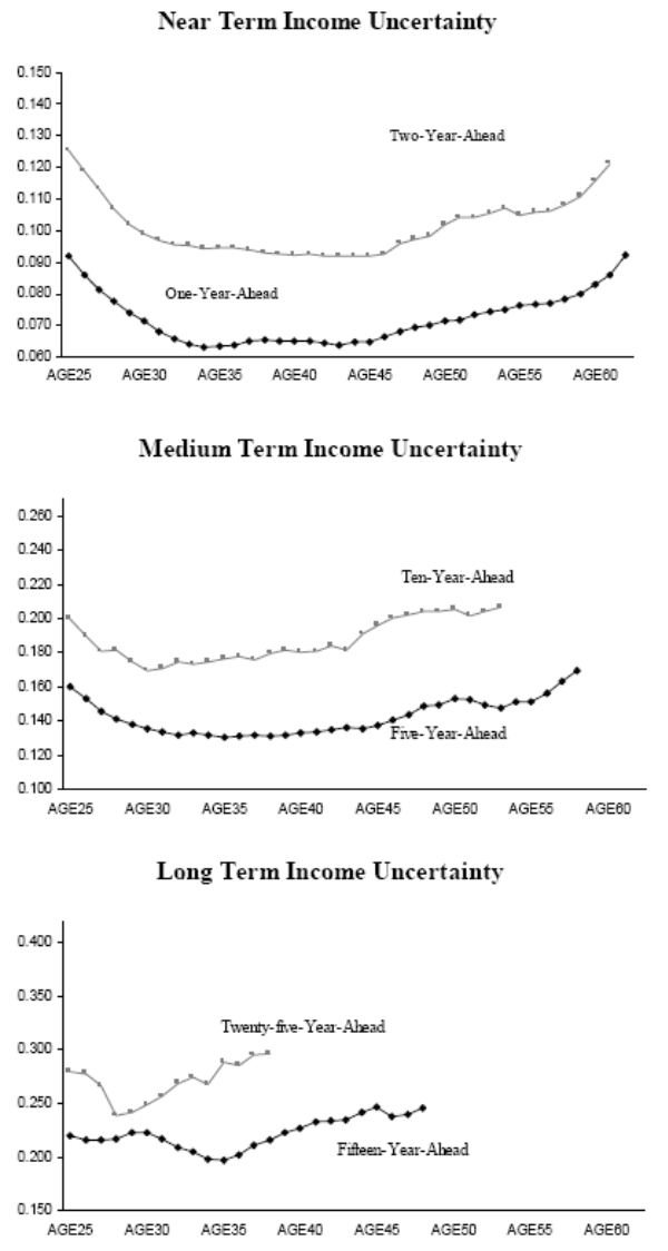
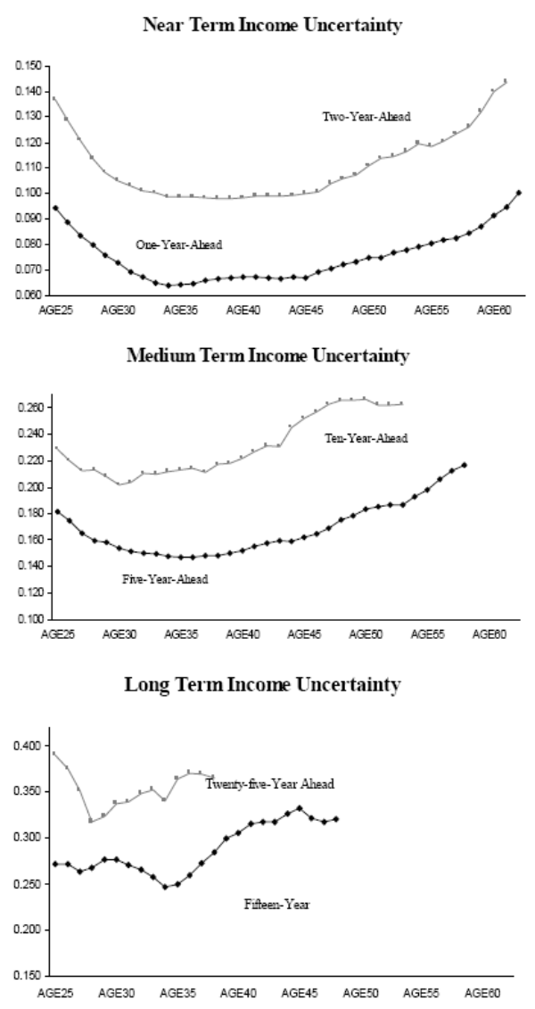
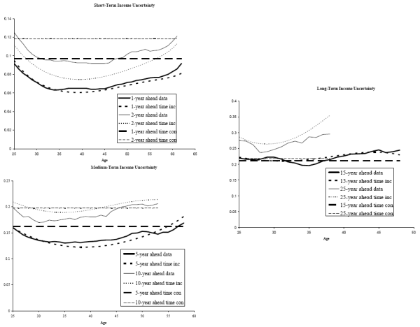
![]() 9. Figures 1 and 2 present several lifecycle income uncertainty profiles at various forecast horizons. Figure 1 plots the AIS results and Figure 2 plots the RIS results.
9. Figures 1 and 2 present several lifecycle income uncertainty profiles at various forecast horizons. Figure 1 plots the AIS results and Figure 2 plots the RIS results.
|
|
We first focus on the AIS results. The top panel of Figure 1 shows near-term income uncertainties. Not surprisingly, the level of uncertainty regarding the two-year-ahead income is higher than the uncertainty associated with the one-year-ahead income. Apart from the magnitude, both uncertainty profiles share a similar U-shaped pattern over the lifecycle. Income uncertainty is high when consumers are in their mid to late twenties. Income uncertainty continues to decline through the mid thirties. After that uncertainties stay at a relatively stable level before rising again in the mid forties. This rise continues into ages close to retirement. The ratio between the maximum and minimum uncertainties over the lifecycle (the max-min ratio) is 1.46 for the one-year-ahead income and 1.37 for the two-year ahead income.
Similar, but less pronounced, U-shaped profiles repeat in the middle panel, which shows medium-term income uncertainties. The uncertainty associated with the five-year-ahead income hits bottom in the mid thirties and stays quite flat until the mid forties. The uncertainty profile of the ten-year-ahead income also exhibits a U-shape, but it bottoms at a somewhat earlier age. In addition, the max-min ratio is 1.30 for the five-year horizon and 1.22 for the ten-year horizon. Both are appreciably lower than the max-min ratios of uncertainties at nearer horizons.
Finally, income-uncertainty profiles at remote horizons, e.g. fifteen and twenty-five years ahead, are plotted in the bottom panel. These curves also show appreciable U-shaped patterns. Because of the age restrictions we impose, these uncertainty profiles cover a much shorter age-span. The max-min ratios are 1.25 for both series, lower than the ratio in the near term.
Now turn to Figure 2, the RIS results. Three features of this figure are noteworthy. First, the contours of these life cycle income uncertainty profiles are very similar to those in the AIS results, shown in Figure
1. Second, because these future income projections are conditioned on a smaller and more restrictive information set, the RIS forecast error variances are greater than the AIS variances across all forecast horizons and for consumers of all ages. Third, the discrepancy
between the RIS and the AIS results widen with the forecasting horizon, ![]() . On average, the RIS one-year-ahead uncertainty is only 4% higher than the AIS uncertainty, whereas the margin is
above 30% at the twenty-five-year horizon. This is not surprising because the difference between
. On average, the RIS one-year-ahead uncertainty is only 4% higher than the AIS uncertainty, whereas the margin is
above 30% at the twenty-five-year horizon. This is not surprising because the difference between
![]() and
and
![]() is what households might know in the base year but which econometricians only observe after a
is what households might know in the base year but which econometricians only observe after a ![]() -year lag. If
-year lag. If ![]() is small, the correlation between the elements in
is small, the correlation between the elements in
![]() and
and
![]() is very high. That is to say the net value of adding
is very high. That is to say the net value of adding
![]() is quite limited. If
is quite limited. If ![]() is large,
is large,
![]() has little predictive power on
has little predictive power on
![]() so introducing
so introducing
![]() adds much more new information and consequently beefs up the forecasting performance.10
adds much more new information and consequently beefs up the forecasting performance.10
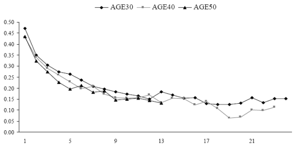
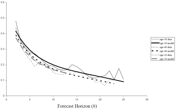
Beside the magnitudes of income uncertainties over the life cycle, we are also interested in the correlations among the stochastic components of income at various horizons. We compute for each age group the correlations between the one-year ahead forecast errors and the forecast errors at other horizons. Figure 3 presents the correlations of consumers that are thirty, forty, and fifty years old in the AIS model. The chart shows that, apart from the longest forecast horizons, the correlations of consumers of various ages are quite similar. We note the following patterns in this graph. First, the correlations decline with the forecast horizon. Second, for all age groups, the correlations between forecast errors at one- and two-year horizons are about the same and slightly below 0.5.
2.5 Robustness Test
To verify whether the U-shaped uncertainty profile over the lifecycle is a spurious consequence of our model specification, sample size, or sample selection, we conduct a series of robustness tests. First, we examine whether the changes in forecast-error variances are due to model misspecification. Remember we project the future income of households of different head ages using the same set of coefficients. If the projection equations should be age-specific and the projection equation we use is closer to the true equations for middle-aged households than to the true equations for younger and older households, the one-size-fit-all approach will reduce fitness for younger and older households and artificially increase income uncertainties for these age groups. We divide our sample into five subgroups by head of household age and reestimate Eqs. (4) and (5) separately for each subgroup. Then we calculate forecast-error variances as we did before and we find the U-shaped uncertainty profiles are qualitatively preserved.
Second, we examine whether changes in the sample size as we vary the forecast horizon (as given inTable 1) might drive the shape of the uncertainty profile. We reestimate the forecast equations using a smaller common sample and reassess income uncertainties over the lifecycle. Apart from the fact that more matrix elements cannot be estimated accurately because of the smaller sample size, the magnitude and dynamics of income uncertainty are very similar to what we presented above.
Finally, we test if our results are driven by low-income households, which are oversampled by the PSID. The core PSID sample consisted of two independent samples - a nationwide representative sample and a sample of low-income families. In the first wave of the survey, the nationwide representative sample has about 3,000 households and the low-income sample has about 2,000 households. We redo our analysis using only the households in the nationwide representative sample and their offspring. The results are very similar to those obtained using the entire PSID core sample.11
2.6 Discussion and Comparison with Earlier Results
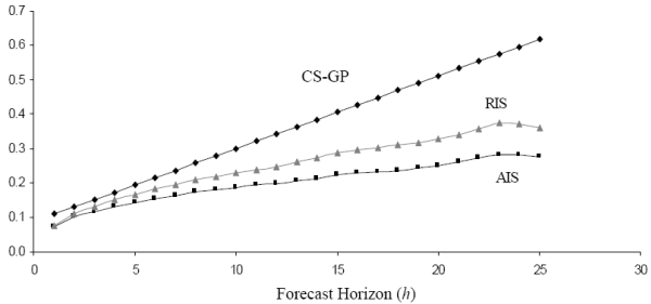
How substantive are the innovations we have introduced into these nonparametric measures of income uncertainty? How different are our results compared to previous results in the literature? We answer this question by contrasting our results to the income uncertainty estimates in the influential work of Carroll and Samwick (1997) and Gourinchas and Parker (2002).
We first briefly review the methodology adopted in Carroll and Samwick (1997) 12. The logarithm of
income, ![]() , is decomposed into a permanent component,
, is decomposed into a permanent component, ![]() , and a transitory
shock,
, and a transitory
shock,
![]() , where
, where ![]() is further assumed to follow a random walk with
predictable income growth
is further assumed to follow a random walk with
predictable income growth ![]() such that
such that
| (6) |
and
noting that the econometrician does not know how either
|
The graph shows that at near horizons, the CS-GP uncertainty estimates are about 30% to 40% greater than the estimated income uncertainty under the AIS assumptions, and 15% to 20% greater than estimates under the RIS assumptions. The gap widens substantially at farther horizons. Beyond a twenty-year horizon, the CS-GP variance estimates more than double the AIS estimates and are over 50% higher than the RIS estimates.
2.7 Summary of Empirical Findings
We construct a nonparametric measure of income uncertainty and study its dynamics over the lifecycle. Our estimates of income uncertainty are typically smaller than previous studies have documented. Our estimates also imply less persistence in income shocks. Over the lifecycle, we find robust U-shaped patterns in the evolution of income uncertainty. Young and old consumers on average have more risky future income relative to middle-age consumers. This U-shaped pattern is robust to a number of sample and model specifications and prevails at almost all horizons.
3.1 Existing Theory of the Consumption Hump
Modern consumption theory begins with the standard Rational-Expectations Lifecycle/Permanent-Income Hypothesis: if consumers are rational then they should allocate consumption over the lifecycle in such a way as to maximize lifetime utility rather than according to simple rules of thumb, such as to consume a constant fraction of disposable income. Thurow (1969) first noted that empirical patterns of lifecycle consumption are hump-shaped and quite similar to the profile of income over the lifecycle. On the face of it, this would appear to refute the RE-LCPIH. However, there are several modifications to the standard model that can account for a hump-shaped consumption profile.14 Each of these modifications introduces testable predictions outside the realm of nondurable consumption. It is an open question how well competing models can simultaneously account for the mean dynamics of lifecycle consumption and the relevant data from other areas of economics, especially since different modifications do not necessarily complement each other.
Often studied in conjunction with borrowing constraints, precautionary saving is the most popular explanation for the consumption hump and the one we focus on in this paper. Precautionary saving will arise if we dispense with the assumption of complete markets so agents are unable to perfectly insure themselves against idiosyncratic risk (Leland (1968), Sandmo (1970)). Nagatani (1972) first suggested that precautionary saving would reduce consumption early in the lifecycle, and Skinner (1988) and Feigenbaum (2008b) have fleshed out how the growth rate of mean consumption from one period to the next increases with income uncertainty. Consequently, if income uncertainty decreases over the lifecycle, this will lead to a concave consumption profile. Using previous measures of uncertainty as described in Section 2.1, several researchers, including Carroll (1997), Carroll and Summers (1991), Gourinchas and Parker (2002), and Hubbard, Skinner, and Zeldes (1994), have documented with calibrated partial-equilibrium models that a combination of borrowing constraints and precautionary saving can produce a hump-shaped consumption profile similar to the data. Feigenbaum (2007) showed that, in general equilibrium, precautionary saving could better account for the hump absent no-borrowing constraints with Gourinchas and Parker's (2002) specification of the income process, which in particular assumes that permanent income shocks are highly persistent and follow a unit-root process.
Nevertheless, precautionary saving is far from the only explanation for a hump-shaped consumption profile, but it is the only one that crucially depends on income uncertainty, which is why it is essential to document precisely how much income uncertainty consumers actually face. Continuing the exploration of incomplete markets, Fernandez-Villaverde and Krueger (2005) have established there is also a hump in durable-goods consumption, and they have found that if durable goods have to be used as collateral for loans then the need to purchase durable goods before borrowing can also produce a hump-shaped profile for consumption of both types of goods. Heckman (1974) and Becker and Ghez (1975) suggested that if leisure and consumption are substitutes then a hump-shaped profile of wages over the lifecycle would induce a hump-shaped profile of consumption. This mechanism also has the side effect of a hump-shaped profile of labor hours, but Bullard and Feigenbaum (2007) recently found there are reasonable calibrations that can match both the consumption hump and the labor-hours profile. Time-varying mortality risk can also explain the hump (Feigenbaum (2008a), Hansen and Imrohoroglu (2006)), though only for a specific set of parameters.
The difficulty of separating out the individual effects of age and other confounding variables means that some portion of the consumption hump may be artificial and due to measurement error. Attanasio et al (1999) and Browning and Ejrnæs (2002) have argued that variations in household size over the lifecycle could play such a confounding role while Aguiar and Hurst (2003, 2007) have shown that the substitution of home production for market consumption may also vary with age.
Of course, a consumption hump can also arise if we abandon the assumption of perfectly rational decision-makers with time-consistent models. Laibson (1997) proposed that hypergeometric discounting could explain the hump while Caliendo and Aadland (2004) have shown that if households can only make plans over a ten- to twenty-year horizon then this can also account for the hump. While the main purpose of this paper is to study the lifecycle dynamics of income uncertainty and its impact on precautionary saving, the theoretical model we introduce in the next section also, for practical reasons, has an element of time-inconsistency.
3.2 The Model
Our characterization of uncertainty, detailed in Section 2, is fundamentally nonparametric since we only measure moments of the income process and do not estimate a parametric specification. Defining uncertainty in nonparametric terms has the advantage that our results are model-independent, but it has the disadvantage that we have no ready-made model of the income process that can be incorporated into lifecycle behavioral models. If we ignore the correlation data we have collected, we could suppose that the income process is simply a sequence of independent shocks with variances given by our volatility matrix. However, it is well established that, for plausible calibrations of utility, income uncertainty will only have a significant impact on consumption and saving if income shocks are persistent (Skinner (1988)). It is not enough for the realization of income to be an uncertain event. Shock in earlier periods have to reveal prior information about this income, so each piece of information the household anticipates it will receive about this income carries some uncertainty also (Feigenbaum (2008b)). It is the combined effect of all these information shocks that accounts for the large effects of precautionary saving in models such as Feigenbaum (2007) or Gourinchas and Parker (2002). In order for income in one year to convey information about income in later years, these income shocks must be dependent.
In a rational expectations model, a household will, by definition, use Bayes' Rule to update its beliefs about the future as its income path is revealed. This requires a complete specification of the probability for every possible income history. Calibrating a time-consistent model that matches our volatility and correlation matrices is a complicated, multidimensional problem that we eschew in this paper. Instead, we calibrate a separate Markov process for each age group that describes how the household believes its income will evolve from that period on. The income process for each age group is calibrated to match the moments of forecast errors for that age group, but we do not impose any restrictions on the collection of these processes that would be necessary to insure time-consistent expectations. Thus we allow households to have time-inconsistent expectations.
We consider a partial-equilibrium model with a consumer who lives for ![]() working periods and
working periods and ![]() retirement periods. For each age
retirement periods. For each age
![]() , the consumer believes future income is determined by a stochastic process that matches the moments obtained from age-
, the consumer believes future income is determined by a stochastic process that matches the moments obtained from age-![]() income forecasts, and we do not require these beliefs to be consistent with Bayes' Law. Let
income forecasts, and we do not require these beliefs to be consistent with Bayes' Law. Let ![]() be the expectation operator with
respect to the consumer's beliefs at age
be the expectation operator with
respect to the consumer's beliefs at age ![]() . An age-
. An age-![]() consumer then maximizes
consumer then maximizes
![\displaystyle E^{(t)}\left[ \sum_{s=t}^{T_{w}-1}\beta^{s-t}u(\widetilde{c}_{s}% (t);\gamma)+\beta^{T_{W}-t}V_{T_{w}}(\widetilde{x}_{T_{w}}(t))\right] ,](img69.gif)
![\displaystyle u(c;\gamma)=\left\{ \begin{array}[c]{cc}% \frac{c^{1-\gamma}}{1-\gamma} & \gamma\neq1\ \ln c & \gamma=1 \end{array} \right.%](img71.gif)
for
Let us suppose an age-![]() consumer believes income at age
consumer believes income at age ![]()
![]() , can take on one of
, can take on one of ![]() values
values
![]() . We assume the probability distribution is a first-order Markov process with transition probabilities
. We assume the probability distribution is a first-order Markov process with transition probabilities
for
To compute aggregates for the population, we must also specify the actual probability distribution for income. We assume, for
![]() , that actual income at
, that actual income at ![]()
![]() , where
, where
for
Households can reallocate income across the lifecycle using the one intertemporal asset in the economy, a risk-free bond that pays the fixed gross interest rate ![]() . Let
. Let
![]() denote the quantity of bonds an agent at age
denote the quantity of bonds an agent at age ![]() plans to purchase at age
plans to purchase at age
![]() that would then pay
that would then pay
![]() at age
at age ![]() . Thus the budget constraint an agent at age
. Thus the budget constraint an agent at age ![]() expects to face at age
expects to face at age ![]() is
is
Since our intent is to focus on the ability of uncertainty and precautionary saving to explain the consumption hump, we allow borrowing but with full commitment to debt contracts. Since consumption is required to be nonnegative, the consumer faces
the endogenous borrowing limit (Aiyagari (1994)) that he would never borrow more than the minimum possible present value of income he might earn in the future, i.e. the minimum that he could possibly pay back in the future. However, there is potentially a disconnect between what the consumer
believes this borrowing limit is and what the borrowing limit actually is. At age ![]() an agent will believe at age
an agent will believe at age ![]() that the borrowing limit he faces is
that the borrowing limit he faces is
 .
. Thus, given ![]() and
and ![]() ,
the consumer's problem at age
,
the consumer's problem at age ![]() is
is
![\displaystyle \max\limits_{\{c_{s}(t)\}_{s=t}^{T_{W}-1},\{b_{s+1}(t)\}_{s=1}^{T_{W}-1}}% E_{t}\left[ \sum_{s=t}^{T_{w}-1}\beta^{s-t}u(\widetilde{c}_{s}(t);\gamma )+\beta^{T_{W}-t}v_{T_{w}}(R\widetilde{b}_{T_{w}}(t))\right] %](img107.gif)
subject to
To simulate the model, at age
Virtually every theoretical explanation for the hump described in Section 3.1 can quantitatively account for the hump if both the interest rate ![]() and discount factor
and discount factor ![]() are free parameters to be calibrated. Bullard and Feigenbaum (2007) and Feigenbaum (2008a) have emphasized the importance of
studying the consumption hump with general-equilibrium models that put some discipline on the choice of
are free parameters to be calibrated. Bullard and Feigenbaum (2007) and Feigenbaum (2008a) have emphasized the importance of
studying the consumption hump with general-equilibrium models that put some discipline on the choice of ![]() and
and ![]() . Since our actual income process is chosen for convenience rather than empirical veracity and the market-clearing interest rate will be very sensitive to the actual income process, we do not endogenize
. Since our actual income process is chosen for convenience rather than empirical veracity and the market-clearing interest rate will be very sensitive to the actual income process, we do not endogenize ![]() . The purpose of the theoretical exercise that follows is to see whether, for any plausible values of
. The purpose of the theoretical exercise that follows is to see whether, for any plausible values of ![]() ,
, ![]() , and
, and ![]() , there is sufficient uncertainty to generate enough precautionary saving to
replicate the consumption hump.
, there is sufficient uncertainty to generate enough precautionary saving to
replicate the consumption hump.
3.3 Specification for the Income Process
Suppose that at age ![]() , the consumer believes for
, the consumer believes for ![]() that
that
where
Note that the income specification of (12) differs from the standard specification of Carroll and Samwick (1997) and Gourinchas and Parker (2002) in two important respects. First, the permanent shocks do not follow a unit-root process, although this
modification is less remarkable since many papers in the literature have considered an AR(1) income process, including Feigenbaum (2008b) and Huggett (1996). The second and more important difference is that the variance of the permanent shocks depends on the age ![]() when forecasting occurs while the variance of the temporary shocks depends both on
when forecasting occurs while the variance of the temporary shocks depends both on ![]() and the forecasting horizon
and the forecasting horizon
![]() .
.
We assume that ![]() is consistent across different ages since we are focusing on changes in the perception of the variance of income
rather than on changes in the perception of the mean. We also assume that the autocorrelation
is consistent across different ages since we are focusing on changes in the perception of the variance of income
rather than on changes in the perception of the mean. We also assume that the autocorrelation ![]() is consistent across ages. This is consistent with Fig. 3,
which shows that the correlation between one-year ahead forecasts and
is consistent across ages. This is consistent with Fig. 3,
which shows that the correlation between one-year ahead forecasts and ![]() -year ahead forecasts is essentially independent of age.18
-year ahead forecasts is essentially independent of age.18
Thus
 |
||
Thus
![\displaystyle V[\ln y_{t+h}(t)\vert y_{t}]=\frac{1-\rho^{2h}}{1-\rho^{2}}\sigma_{p}^{2}% (t)+\sigma_{zh}^{2}(t)+\rho^{2h}\sigma_{z0}^{2}(t) %](img133.gif)
For
To discretize this process, we restrict
![]() to take on values such that
to take on values such that
for
for
where
Note that this specifies the time-inconsistent probability distribution as perceived by the household. We must also specify the Markov process of the actual probability distribution for realized income ![]() . As described above, we assume that the household's perceptions of its current temporary and permanent shocks are correct, so
. As described above, we assume that the household's perceptions of its current temporary and permanent shocks are correct, so
This implies the set of actual income states for
Let
![]() denote the invariant distribution of
denote the invariant distribution of ![]() . We then assume the
actual probability distribution of
. We then assume the
actual probability distribution of ![]() is
is
3.4 Calibration
For the income process, we assume both the permanent and temporary shocks are governed by two-state processes.19 The temporary shocks are parameterized by
![]() and
and
![]() . Likewise, the permanent shocks are parameterized by
. Likewise, the permanent shocks are parameterized by
![\begin{displaymath} \Pi^{p}=\frac{1}{2}\left[ \begin{array}[c]{cc}% 1+\rho & 1-\rho\ 1-\rho & 1+\rho \end{array}\right] . \end{displaymath}](img182.gif)
We calibrate ![]() ,
,
![]() , and
, and
![]() so as to minimize the distance of the correlation and volatility matrices relative to their predicted values from (13) and (14). Specifically, we parameterize the permanent-shock standard deviation as a
so as to minimize the distance of the correlation and volatility matrices relative to their predicted values from (13) and (14). Specifically, we parameterize the permanent-shock standard deviation as a ![]() -degree polynomial
-degree polynomial
and the temporary-shock standard deviation as a tensor product of
Then we set
In Section 2, we measure the volatility and correlation matrices for horizons up to
![]() . For
. For
![]() we will also need to specify
we will also need to specify
![]() for
for
![]() , but these standard deviations are not identified by the available data. We will consider what happens both if we linearly extrapolate (19) for
, but these standard deviations are not identified by the available data. We will consider what happens both if we linearly extrapolate (19) for
![]() and if we assume a flat extrapolation where
and if we assume a flat extrapolation where
![]() for
for
![]() . We also do not have information about
. We also do not have information about
![]() since we have no data at forecasts in the last working period. However, we do have the volatility matrix element
since we have no data at forecasts in the last working period. However, we do have the volatility matrix element
![]() , so it is reasonable to assume (19) will still be valid at
, so it is reasonable to assume (19) will still be valid at ![]() . Likewise, we simply extrapolate (18) to obtain
. Likewise, we simply extrapolate (18) to obtain
![]() .
.
We consider the nonparametric estimates obtained with both the AIS and RIS specifications of Section 2 with a cubic approximation that sets
![]() . To assess the importance of the age and forecast-horizon dependence of uncertainty we also consider a time-consistent calibration of the income process where
. To assess the importance of the age and forecast-horizon dependence of uncertainty we also consider a time-consistent calibration of the income process where
![]() and
and
![]() are constants independent of
are constants independent of ![]() and
and ![]() . Thus the time-consistent income process falls into the class of Markov income processes that have previously been studied in the literature (for example in Feigenbaum (2008b) and Huggett (1996)). The time-consistent
calibration is obtained, both for the AIS and RIS specifications, as above but with
. Thus the time-consistent income process falls into the class of Markov income processes that have previously been studied in the literature (for example in Feigenbaum (2008b) and Huggett (1996)). The time-consistent
calibration is obtained, both for the AIS and RIS specifications, as above but with
![]() .
.
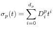
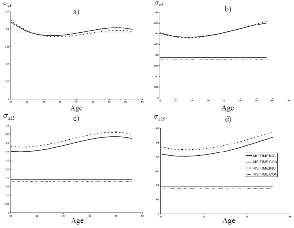
The time-inconsistent and time-consistent calibrations of
![]() are plotted as a function of age
are plotted as a function of age ![]() in Fig. 5 for
both the AIS and RIS specifications. Likewise, the four calibrations of
in Fig. 5 for
both the AIS and RIS specifications. Likewise, the four calibrations of
![]() are plotted as a function of age for representative horizons in Fig. 6. The correlation for each calibration is given in Table 3. The variance of permanent income shocks is uniformly larger for the time-consistent calibration than the time-inconsistent calibration, and for most horizons the time-consistent variance is twice as large as the time-inconsistent variance. The correlations for the
time-consistent calibrations are modestly smaller than the corresponding time-inconsistent calibrations. At short time horizons the variance of temporary income shocks is comparable between the time-consistent and time-inconsistent calibrations, but the variance of temporary income shocks increases
with the forecast horizon in the time-inconsistent model while necessarily remaining constant in the time-consistent model. Thus permanent income shocks will have greater emphasis in the time-consistent models whereas temporary income shocks will have more emphasis in the time-inconsistent
models.
are plotted as a function of age for representative horizons in Fig. 6. The correlation for each calibration is given in Table 3. The variance of permanent income shocks is uniformly larger for the time-consistent calibration than the time-inconsistent calibration, and for most horizons the time-consistent variance is twice as large as the time-inconsistent variance. The correlations for the
time-consistent calibrations are modestly smaller than the corresponding time-inconsistent calibrations. At short time horizons the variance of temporary income shocks is comparable between the time-consistent and time-inconsistent calibrations, but the variance of temporary income shocks increases
with the forecast horizon in the time-inconsistent model while necessarily remaining constant in the time-consistent model. Thus permanent income shocks will have greater emphasis in the time-consistent models whereas temporary income shocks will have more emphasis in the time-inconsistent
models.
|
|
For the AIS estimates, the root-mean-squared deviation between the time-inconsistent model's predictions for the volatility and correlation matrices and the corresponding empirical estimates is 0.022. For the time-consistent model, the root-mean-squared deviation is 0.051. Fig. 7 shows how the variances of forecast errors for these two models compare to the nonparametric estimates as a function of age at different forecast horizons. Since the time-consistent model assumes that the standard deviation of temporary and permanent income shocks is independent of age, its variance graphs are flat whereas the time-inconsistent model is able to capture the U-shaped dependence of the variances with respect to age. For short horizons of one to two years, the time-consistent model overpredicts the uncertainty at all ages. For long horizons, the time-consistent model significantly underpredicts the uncertainty. Consistent with the root-mean-squared deviations, the time-inconsistent model almost uniformly does better at matching the forecast-error variances, although it does underpredict the variance at the two-year horizon. The comparison is similar for the RIS specification.
|
Fig. 8 shows how the correlations between one-year ahead forecast errors and ![]() -year ahead forecast errors compare
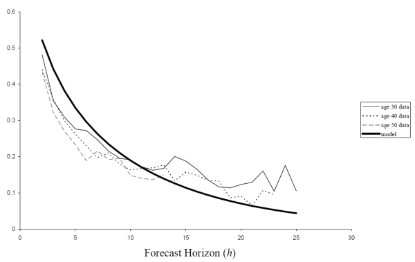
at ages 30, 40, and 50 between the nonparametric estimates and the time-inconsistent income process under the AIS specification. Fig. 9 shows the same comparison for the time-consistent income process. The time-inconsistent model matches the correlations slightly better
as the time-consistent model overpredicts the correlation at short horizons and underpredicts it at long horizons.
-year ahead forecast errors compare
at ages 30, 40, and 50 between the nonparametric estimates and the time-inconsistent income process under the AIS specification. Fig. 9 shows the same comparison for the time-consistent income process. The time-inconsistent model matches the correlations slightly better
as the time-consistent model overpredicts the correlation at short horizons and underpredicts it at long horizons.
|
|
In addition to the income process, we also have to calibrate the preference parameters ![]() and
and ![]() , and since this is a partial-equilibrium model the gross interest rate
, and since this is a partial-equilibrium model the gross interest rate ![]() . Following Feigenbaum (2008b), we set the
discount factor and interest rate to common values from the literature:
. Following Feigenbaum (2008b), we set the
discount factor and interest rate to common values from the literature:
![]() and
and ![]() . Feigenbaum (2007) found that a risk aversion of
. Feigenbaum (2007) found that a risk aversion of
![]() could best account for the lifecycle consumption profile under Gourinchas and Parker's (2002) income process, so we maintain this value.
could best account for the lifecycle consumption profile under Gourinchas and Parker's (2002) income process, so we maintain this value.
3.5 Theoretical Predictions for Consumption Hump
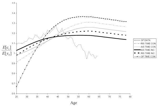
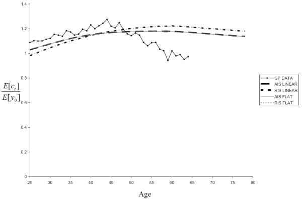
Fig. 10 shows lifecycle profiles for mean consumption (normalized by mean initial income) for the time-inconsistent and time-consistent calibrations under both the AIS and RIS specifications along with Gourinchas
and Parker's empirical measurements of the mean consumption profile20.21 For comparison with the previous literature, we also include the results for a time-consistent model with Gourinchas and Parker's estimates of the shock variances:
![]() and
and
![]() . In their model, the permanent income shocks follow a unit-root process. Since a unit-root process cannot be nested in our model, we set
. In their model, the permanent income shocks follow a unit-root process. Since a unit-root process cannot be nested in our model, we set ![]() . In Table 4, we also report the peak to initial consumption of the lifecycle profile of mean consumption and the age of peak consumption.
. In Table 4, we also report the peak to initial consumption of the lifecycle profile of mean consumption and the age of peak consumption.
|
|
|---|
All five models produce a hump-shaped lifecycle consumption profile for our chosen calibration of the preference parameters and the interest rate. The consumption-saving model with the time-inconsistent income process based on the AIS specification most closely matches Gourinchas and Parker's estimates of mean consumption as a function of age, although this ranking might change with other calibrations.
Our primary interest here lies in the degree to which different measures of uncertainty impact the consumption profile for a given calibration. Since ![]() , in the absence of uncertainty the lifecycle consumption profile should be monotonically decreasing with a peak at the initial age of 25, so the peak to initial consumption ratio should be 1. Thus the peak to initial consumption ratio can be viewed here as a measure of
how much precautionary saving causes these models to deviate from the LCPIH. Since we are also holding the degree of risk aversion fixed, the variation in precautionary saving over different income processes should reflect the amount of uncertainty faced over the lifecycle under each process.
, in the absence of uncertainty the lifecycle consumption profile should be monotonically decreasing with a peak at the initial age of 25, so the peak to initial consumption ratio should be 1. Thus the peak to initial consumption ratio can be viewed here as a measure of
how much precautionary saving causes these models to deviate from the LCPIH. Since we are also holding the degree of risk aversion fixed, the variation in precautionary saving over different income processes should reflect the amount of uncertainty faced over the lifecycle under each process.
Not surprisingly, since the AIS specification assumes households have more information than the RIS specification, the two AIS models have smaller peak to initial consumption ratios than their corresponding RIS models. Moreover, the Gourinchas and
Parker-based model with its near unit-root process has a substantially larger peak to inital consumption ratio than the four models we estimate since it has the most uncertainty. Indeed, for
![]() and
and ![]() , Gourinchas and Parker (2002) have to dial the risk
aversion all the way down to one half to get a lifecycle consumption profile that resembles the data, but this would not be necessary for our more robust uncertainty measure.
, Gourinchas and Parker (2002) have to dial the risk
aversion all the way down to one half to get a lifecycle consumption profile that resembles the data, but this would not be necessary for our more robust uncertainty measure.
For both the RIS and AIS specifications, we also find that the time-inconsistent model has a significantly smaller peak to initial consumption ratio than the corresponding time-consistent model. This can be explained in terms of Figs. 5 and 6. Because the time-consistent model assumes a constant variance for the permanent and temporary shocks, independent of age and forecast horizon, the time-consistent model needs a large permanent shock variance to best match the volatility and correlation matrices. In contrast, the time-inconsistent model has a smaller permanent shock variance and exploits its ability to increase the temporary shock variance at longer forecast horizons to better match the forecast-error moments. As Constantinides and Duffie (1996) argued, permanent shocks will have a substantially larger impact on the behavior of consumers, and Feigenbaum (2007,2008b) confirm that more persistent income shocks lead to greater precautionary saving. This intuition is further corroborated here. Thus, failing to account for the time and forecast-horizon dependence of uncertainty can bias upward estimates of the importance of precautionary saving.
3.6 Robustness Checks
One cause for concern about the calibration of the income process in Section 3.4 is that we have no data on the variance and correlation of forecast errors beyond a twenty-five-year horizon, but the model requires us to
specify the household's beliefs about income at all future horizons. In Section 3.5, we reported results for the baseline case where we assume a linear extrapolation of Eq. (19) for
![]() . In Fig. 11, we consider what happens with the alternative assumption of a flat extrapolation such that
. In Fig. 11, we consider what happens with the alternative assumption of a flat extrapolation such that
![]() for
for
![]() . For both the AIS and RIS specifications, we find a negligible difference between the two extrapolations. The effect of a temporary income shock twenty-five years in the
future is going to be heavily discounted, so a change in the temporary shock variance at such large horizons has little to no effect on consumption behavior.
. For both the AIS and RIS specifications, we find a negligible difference between the two extrapolations. The effect of a temporary income shock twenty-five years in the
future is going to be heavily discounted, so a change in the temporary shock variance at such large horizons has little to no effect on consumption behavior.
|
Another potential cause for concern about our results is that we use only two-state processes to model both the permanent and temporary income shocks. Would a finer distribution produce different results? Feigenbaum (2008b) suggests that only the
second-order moments should have a significant effect on the shape of the mean consumption profile. Given the common assumption that shocks are normally distributed, the next moment of interest is the kurtosis. For a normal distribution, the kurtosis should be 3. However, an unskewed two-state
process must have the minimum kurtosis of 1. For the temporary shock process, we can easily replicate both the variance and kurtosis of a normal distribution with a three-state process characterized by
![]() and
and ![]() with
with
![]() and
and
![]() . We can also obtain an unconditional distribution of permanent shocks that matches the variance and kurtosis of a normal distribution in this way, but with
. We can also obtain an unconditional distribution of permanent shocks that matches the variance and kurtosis of a normal distribution in this way, but with
![]() we cannot do the same for the conditional distribution of permanent shocks, which is what should matter most for precautionary saving. With three states, the best we can do is
choose a transition matrix that minimizes the kurtosis of the conditional distribution. If the unconditional kurtosis is
we cannot do the same for the conditional distribution of permanent shocks, which is what should matter most for precautionary saving. With three states, the best we can do is
choose a transition matrix that minimizes the kurtosis of the conditional distribution. If the unconditional kurtosis is ![]() , the minimum conditional kurtosis goes as
, the minimum conditional kurtosis goes as
![]() in the limit as
in the limit as
![]() .
.
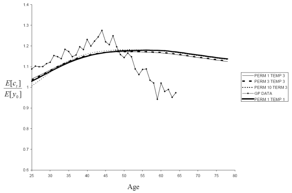
In Fig. 12, we plot the mean consumption profile for the AIS specification of the time-inconsistent model for various choices of ![]() and the kurtosis of the temporary shock distributions. To get a sense of scale, we also plot the empirical profile of Gourinchas and Parker (2002). Three of the model profiles, for which the unconditional kurtoses of both shocks are between 1 and 3, are virtually
indistinguishable. The ratio of peak consumption to initial consumption for all three curves is between 1.125 and 1.146. Only when we increase
and the kurtosis of the temporary shock distributions. To get a sense of scale, we also plot the empirical profile of Gourinchas and Parker (2002). Three of the model profiles, for which the unconditional kurtoses of both shocks are between 1 and 3, are virtually
indistinguishable. The ratio of peak consumption to initial consumption for all three curves is between 1.125 and 1.146. Only when we increase ![]() to 10 do we get any significant
departure, and even then the peak to initial ratio only increases to 1.17. Comparing Fig. 12 to Fig. 10, we see that the impact of using a finer distribution is much smaller than the impact of ignoring the time-dependence of uncertainty or
adding more information to the model.
to 10 do we get any significant
departure, and even then the peak to initial ratio only increases to 1.17. Comparing Fig. 12 to Fig. 10, we see that the impact of using a finer distribution is much smaller than the impact of ignoring the time-dependence of uncertainty or
adding more information to the model.
|
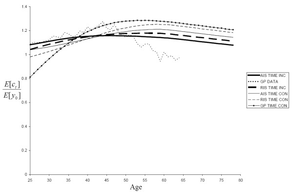
As a final robustness check, let us consider how sensitive the model is to the risk aversion ![]() . In Fig. 13 and
Table 5 we replicate Fig. 10 and Table 4 but for
. In Fig. 13 and
Table 5 we replicate Fig. 10 and Table 4 but for ![]() . We still
get hump-shaped consumption profiles, but not surprisingly with less risk aversion there is less precautionary saving so the humps are more modest in size. Interestingly, while the consumption profile for the AIS specification of the time-inconsistent model now has a peak to initial consumption
ratio smaller than Gourinchas and Parker (2002) find, this calibration does match the age of the peak.
. We still
get hump-shaped consumption profiles, but not surprisingly with less risk aversion there is less precautionary saving so the humps are more modest in size. Interestingly, while the consumption profile for the AIS specification of the time-inconsistent model now has a peak to initial consumption
ratio smaller than Gourinchas and Parker (2002) find, this calibration does match the age of the peak.
|
|
|---|
4 Conclusion
We introduce a new method of measuring income uncertainty and apply the estimates obtained via this approach to investigate the extent to which variations in income uncertainty over the lifecycle could be responsible for the hump-shaped consumption profile. Our measurement technique articulates the distinction between income heterogeneity and uncertainty, and acknowledges that households may have superior information to econometricians. Our estimation reveals an income uncertainty level that is lower than what has been presented in the existing literature and shows that income uncertainty does evolve over the lifecycle in a fashion consistent with conventional wisdom. In addition, we show that for a plausible calibration of the preference parameters, our estimate of income uncertainty does imply a hump-shaped lifecycle consumption profile that matches consumption data very well.
Two lines of research are worth pursuing in the future. First, it is important to study whether we can find a time-consistent, parametric income process consistent with our nonparametic estimates. This is necessary in order to study what happens in general equilibrium for this model. Second, we will study more carefully the source of the variation of income uncertainty over the lifecycle.
A. Computational Procedure
We can write the problem (11) as a recursive sequence of Bellman equations as follows. Let us denote the state variable ![]() such that
such that
![]() . For each base age
. For each base age
![]() , the consumer solves for the age-
, the consumer solves for the age-![]() perceived value functions
perceived value functions
![]() at current and future ages
at current and future ages
![]() . For
. For
![]() , the Bellman equation is
, the Bellman equation is
subject to
where