Skip to: [Printable Version (PDF)] [Bibliography] [Footnotes]

Finance and Economics Discussion Series: 2008-38 Screen Reader version ^♣

Estimating the common trend rate of inflation for consumer prices and consumer prices excluding food and energy prices

Michael T. Kiley¹

July 16, 2008

Keywords: Core inflation, food and energy prices

Abstract

I examine the common trend in inflation for consumer prices and consumer prices excluding prices of food and energy. Both the personal consumption expenditure (PCE) indexes and the consumer price indexes (CPI) are examined. The statistical model employed is a bivariate integrated moving average process; this model extends a univariate model that fits the data on inflation very well. The bivariate model forecasts as well as the univariate models. The results suggest that the relationship between overall consumer prices, consumer prices excluding the prices of food and energy, and the common trend has changed significantly over time. In the 1970s and early 1980s, movements in overall prices and prices excluding food and energy prices both contained information about the trend; in recent data, the trend is best gauged by focusing solely on prices excluding food and energy prices.

JEL Classification: E31, E37

Core inflation is often defined as the trend rate of change in overall prices. The rate of change in consumer prices excluding food and energy prices, perhaps smoothed over several quarters, is a common proxy for this definition of core inflation - reflecting the idea that food and energy prices are more volatile than (most) other components, implying that such prices may contain less signal regarding the trend rate of inflation.²

In a forecast context, projections of overall consumer price inflation often converge to recent values of inflation measured from consumer prices excluding food and energy prices; empirical evidence that overall consumer price inflation may "error correct" toward inflation measured from consumer prices excluding food and energy prices is sometimes presented to motivate this practice.³

This article examines the trend rate of inflation using a simple statistical process of overall consumer prices and consumer prices excluding food and energy prices. The statistical model chosen, an integrated moving average process, has been shown to explain the data very well (see section 1); the innovation herein is to apply this statistical model jointly to the data on overall consumer prices and consumer prices excluding food and energy prices. The analysis allows a simple interpretation of a number of previous results, including: the nature of error correction between inflation in overall consumer prices and consumer prices excluding food and energy prices; second-round effects from food and energy prices to inflation; and the relative performance of various simple forecast models. Moreover, the statistical model provides an estimate of trend inflation.

1. A good statistical model of inflation

The empirical exercises herein will focus on quarterly data for consumer prices and consumer prices excluding food and energy prices. I consider two measures of consumer prices: the personal consumption expenditure price (PCE) index and the consumer price index (CPI); these measures differ somewhat in their coverage and in how they aggregate prices to construct an aggregate price level.

I will define trend inflation as the expected value of inflation over the next four quarters. Defining trend in terms of forecast follows Bryan and Cecchetti (1994). Alternative estimates of trend are evaluated by examining their performance in forecasting inflation.⁴

Evaluation of alternative measures requires a reference model that has good forecast performance. Previous research has shown that univariate statistical models of consumer prices and consumer prices excluding food and energy prices in which the rate of change in these indexes consists of a random-walk trend component and a serially-uncorrelated transitory component perform very well - implying that inflation follows an integrated moving average (IMA(1,1)) process. For example, Stock and Watson (2007, 2008) show that such univariate models outperform (for forecasting) other univariate models and statistical models that include other predictors (such as measures of activity, interest rates, etc.).⁵ Earlier work, including Nelson and Schwert (1977) and Barsky (1987), reached similar conclusions on the univariate properties of inflation. Stock and Watson (2007, 2008) emphasize the importance of variation in the volatility of the permanent and transitory components of inflation.

This statistical model implies that trend inflation is an exponentially-weighted average of past realizations. Interestingly, Muth (1960) suggested that forecasts from such models would be optimal in some contexts in work that accompanied his research on rational expectations.⁶

Previous research has used this statistical model on overall consumer prices and consumer prices excluding food and energy prices separately. I propose modeling these data jointly. Specifically, I assume that overall consumer prices and consumer prices excluding food and energy prices share a common trend component; the transitory components are allowed to be correlated. These assumptions exclude the possibility of a trend in food and energy prices relative to other prices; whether this exclusion impairs forecast performance will be apparent in the evaluation below.

The joint model (1) is given by

p(t) = p*(t) + u(t)
pxfe(t) = p*(t) + w(t), [u(t), w(t)] ? $\sim$ N(0,S)
p*(t) = p*(t-1) + e(t), e(t) $\sim$ N(0, v),

(1)

where p(t) is the log-difference in overall consumer prices, pxfe(t) is the log-difference in consumer prices excluding food and energy prices, p*(t) is the common trend, and u(t), w(t), and e(t) are serially uncorrelated shocks; the matrix S is the variance covariance matrix of the transitory shocks (u and w) and v is the variance of the permanent shock (e). This is a model in which both measures of inflation follow correlated IMA(1,1) processes.

I have not indexed the second moments of the shocks (e.g., the variance-covariance matrix S and the variance v) by time period. Stock and Watson (2007, 2008) emphasize the importance of variation over time in the size of permanent and transitory shocks; in particular, they find that the variance of permanent shocks relative to transitory shocks was much larger in the late 1970s and early 1980s than in subsequent years, consistent with the idea the period surrounding the Volcker disinflation was one of substantially swings in trend inflation. I allow for this time variation by estimating the model using rolling windows of 60 quarters; this is one of the strategies followed by Stock and Watson (2007).

The joint model (1) is compared to two univariate models with the same structure - that is, the separate models of overall consumer prices and consumer prices excluding food and energy prices presented in Stock and Watson:

p(t) = p*(t) + u(t), u(t) ? $\sim$ N(0,s)
p*(t) = p*(t-1) + e(t), e(t) $\sim$ N(0, v),

(2)

pxfe(t) = p*(t) + w(t), w(t)

N(0,s)
p*(t) = p*(t-1) + e(t), e(t)

N(0, v)

(3)

In addition, I consider the proposal for trend inflation presented in Atkeson and Ohanian (2001) - equal to the four-quarter moving average of either overall consumer price inflation or inflation in consumer prices excluding food and energy prices.

2. Results

Each model (1 through 3) is estimated using a rolling 60-quarter window. The initial sample is 1960Q1 to 1974Q4. This sample is used to estimate the trend rate of inflation for the period after 1974Q4, and performance is evaluated using the forecast error over the subsequent four quarters (i.e., inflation over the four quarters to 1975Q4). The sample is then rolled forward one period (i.e., to 1960Q2 to 1975Q1), the model is re-estimated, and the trend estimates are produced. The entire evaluation period is based on forecasts produced from 1974Q4 to 2006Q4 (based on realizations of four-quarter inflation from 1975Q4 to 2007Q4).

All of the results reported in the rest of the memo are very similar across the PCE index and the CPI. I present the results for the PCE index first, and then report the same set of information for the CPI. Because the results are so similar across the alternative indexes, the second discussion - of the CPI results - is less detailed.

Personal Consumption Expenditure (PCE) Price Index

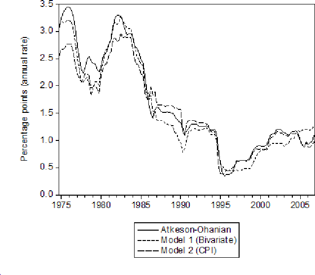
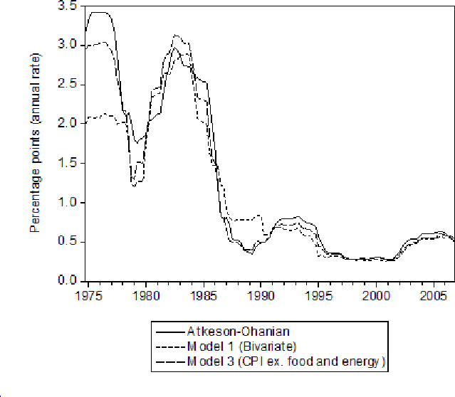
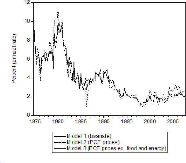
The trend estimates produced by models 1 to 3 applied to PCE prices are presented in figure 1. (As outlined above, these are the one-sided trend estimates derived from the model based on the rolling 60-quarter parameter estimates). It is clear that the trend estimate from model 1 - the joint model of overall PCE prices and PCE prices excluding food and energy prices - is fairly similar to that from the model 3 (the model of PCE prices excluding food and energy prices only), especially in recent years. The section on interesting economic results below will examine how the similarity between the estimate of trend from the joint (bivariate) model and the univariate model of prices excluding food and energy prices is related to previous work on error-correction and pass-through of food and energy prices to other prices in some detail. For now, I note the estimates of trend inflation in 2007Q4 from each model (at an annual rate):

Model 1 (joint model of both indexes): 2.2 percent
Model 2 (overall PCE): 2.7 percent
Model 3 (PCE ex. food & energy): 2.1 percent

From a forecast perspective, it clearly matters a great deal which model is chosen: The inflation outlook differs by more than $\raise.5ex\hbox{$\scriptstyle 1$}\kern-.1em/ \kern-.15em\lower.25ex\hbox{$\scriptstyle 2$}$ percentage point across the three models.

Table 1 presents results on forecast accuracy for models 1, 2, and the Atkeson-Ohanian model for overall PCE prices; Table 2 presents the same information for PCE prices excluding food and energy prices. The results are presented for the entire sample (1974Q4 to 2006Q4) and for subsamples, where the entire sample is divided into thirds. The results in these tables suggest three conclusions:

The trend estimates from all of the IMA(1,1) models dominate the Atkeson-Ohanian measure (the most recent four-quarter change) for overall PCE prices in all samples. For core prices, the IMA(1,1) models perform better than the Atkeson-Ohanian measure for the entire sample, but the Atkeson-Ohanian measure dominates for the most recent two sub-samples;
The joint model of overall prices and prices excluding food and energy prices are sometimes better than the univariate models proposed by Stock and Watson (2007, 2008);
Most importantly, the differences are very small in recent periods.

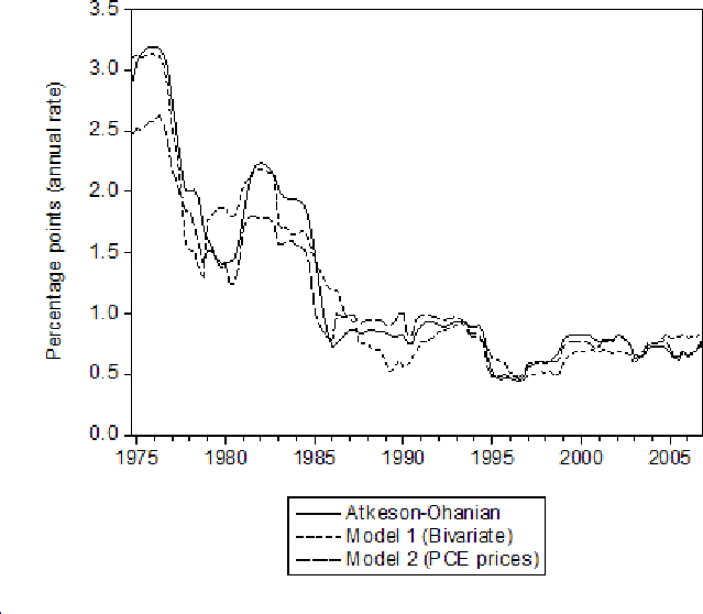
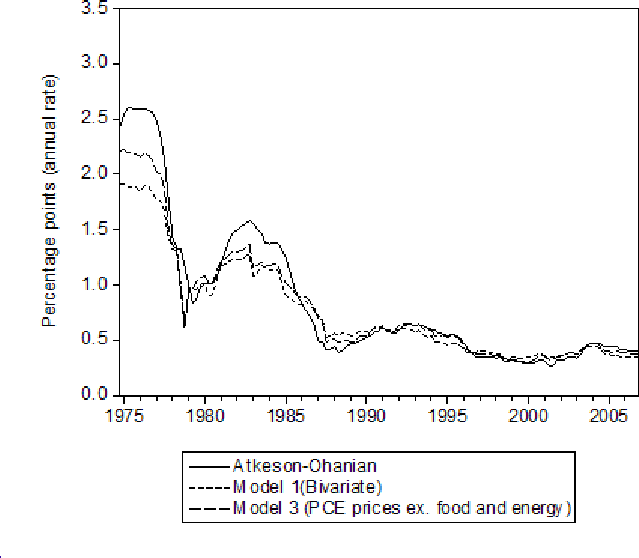
These conclusions are apparent in figures 2 and 3, which present the root mean square error over the 16 quarters prior to the date shown for overall prices and prices excluding food and energy prices for the IMA(1,1) models and the Atkeson-Ohanian model. The relative performance of various models changes over time somewhat. But the dominant impression from both figures is that the RMSEs in recent years are small and similar across each specification. This is essentially the conclusion of Stock and Watson (2007, 2008), which show that the univariate IMA(1,1) is as good as most alternatives, the size of forecast errors has fallen since the 1970s, and the amount of forecastable variation in inflation has been low in recent years.

Consumer Price Index (CPI)

The same set of figures and tables are presented for the CPI. These results show the following:

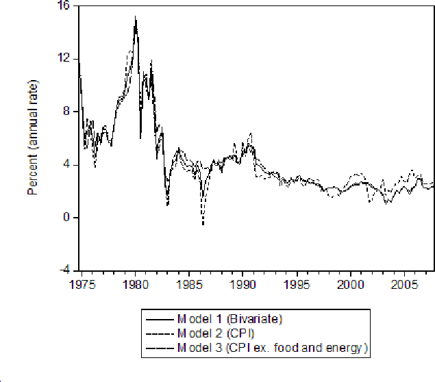
The estimated trend from the bivariate IMA(1,1) model for the CPI looks very similar to the trend from the univariate model of the CPI excluding food and energy prices, especially in recent years (figure 4). The estimated trends at an annual rate for 2007Q4 for the bivariate model equaled 2.4 percent; for the univariate model of overall prices equaled 2.8 percent; and for the univariate model of prices excluding food and energy prices equaled 2.4 percent.
The forecast performance of the different models varies over time. The bivariate IMA(1,1) model dominates the univariate models for some periods. But the differences in forecast performance are very small in recent years. (Each of these conclusions can be gleaned from tables 3 and 4 and figures 5 and 6).⁷

3. Some interesting economic results

The results in the last section - especially the finding that the joint modeling of overall prices and prices excluding food and energy prices has similar forecast performance to the univariate models of Stock and Watson (2007, 2008) - beg the question of whether our empirical exploration of a bivariate model is worth the effort. There are some interesting insights that follow from the joint modeling of overall prices and prices excluding food and energy prices.

In particular, these models fit the data well, as in Stock and Watson (2007, 2008), yet allow consideration of three important (and highly interrelated) questions that cannot be answered using the univariate approach of these authors (and others, e.g., Cogley (2002)). The questions are

What is the information content on overall prices and prices excluding food and energy prices for the trend in inflation?
How is the information content in each measure related to previous findings on error-correction of overall inflation to inflation measured from prices excluding food and energy prices?
How is the information content in each measure related to previous findings on the pass-through of energy or food inflation to inflation of other prices?

I examine each of these questions in turn.

The information content in overall prices and prices excluding food and energy prices for trend inflation

Applying the Kalman filter to model 1, the estimate of the trend (p*_(t)) is related to the data on overall inflation and inflation measured from prices excluding food and energy prices via the following formula:

p*_(t)-p*_(t-1) = a1*(p(t)-p*_(t-1)) + a2* (pxfe(t)-p*_(t-1)).

The coefficients a1 and a2 reflect the relative information content of overall prices and prices excluding food and energy prices and are determined by the following set of equations (which determine a1, a2, and $\Sigma$ , the variance of the gap between the estimated trend and true trend):

$\Sigma \quad -$ a1*( $\Sigma$ +S $_{11})$ - a2*( $\Sigma$ +S $_{11})$ = 0

$\Sigma \quad -$ a1*( $\Sigma$ +S $_{12})$ - a2*( $\Sigma$ +S $_{22})$ = 0

$\Sigma \quad -$ (1-a1-a2)²* $\Sigma$ - a1²* S $_{11}$ - a1*a2*S $_{12}$ - a2²* S $_{22}$ - v = 0,

where (from model 1) v is the variance of the permanent shock and S $_{11}$ , S $_{12}$ , and S $_{22}$ are the elements of the variance-covariance matrix (S) of transitory shocks.⁸ For example, a1 is low if the variance of the transitory shock to overall prices (S $_{11})$ is high relative to the variance of the shock to prices excluding food and energy prices (S $_{22})$ (ceteris paribus); a1 and a2 are both low if the variance of the permanent shock (v) if low relative to the variances of the transitory shocks (S $_{11}$ , S $_{22})$ .

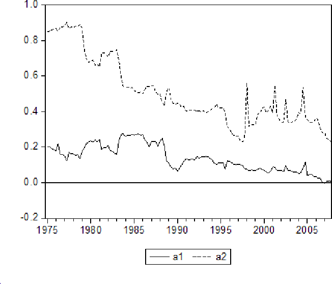
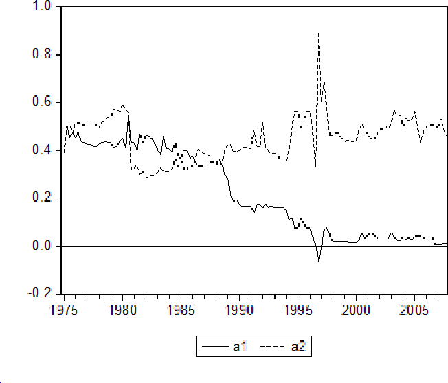
Figure 7 presents the values for a1 and a2 implied by the coefficients for each sample used in the rolling estimation procedure outlined in the previous section using the PCE price index; figure 8 presents the values of a1 and a2 for the CPI. The results are stark.

Surprises in both overall inflation and inflation measured using prices excluding food and energy prices in the mid-1970s had significant information; for the CPI, the weights on overall inflation and inflation measured from prices excluding food and energy prices were approximately equal (and near $\raise.5ex\hbox{$\scriptstyle 1$}\kern-.1em/ \kern-.15em\lower.25ex\hbox{$\scriptstyle 2$} )$ through the mid-to-late 1980s.
The most recent data suggest that surprises in overall inflation have had no information for trend inflation (a1 near zero); all of the information regarding trend has been contained in prices excluding food and energy prices.
The combined information in inflation measures (a1 + a2) in recent samples is clearly below the values that prevailed prior to and just after the Volcker disinflation. This result is similar to the finding in Stock and Watson (2007, 2008) that the variance of permanent shocks has fallen since the Volcker period.

The evolving information content in overall prices and prices excluding food and energy prices provides some support to a focus on prices excluding food and energy prices in a policy context (e.g., as discussed in Mishkin (2007)), despite the small differences in forecast performance in recent years. Of course, this is a feature of the reduced form for inflation and undoubtedly depends on the nature of monetary policy reactions to inflation.

Error-correction of inflation in overall prices to inflation of prices excluding food and energy prices

A number of studies have found that the rate of change in overall PCE prices error corrects to an estimate of inflation based on prices excluding food and energy prices (e.g., Blinder and Reis (2005)). Policymakers have referred to this tendency in discussing the outlook for inflation (e.g., Rosengren (2008)).

Blinder and Reis (2005) estimate regressions of the following form

p(t+h,t)-p(t) = c1*(p(t)-pxfe(t)) + e1(t)

pxfe(t+h,t)-pxfe(t) = c2*(pxfe(t)-p(t)) + e2(t)

where p(t+h,t) is the rate of inflation on overall prices averaged between period t+h and t (and similarly for pxfe(t+h,t)) and the other variables are as defined earlier. A tendency of overall inflation to correct to the measure estimated excluding food and energy prices implies that c1 is less than zero; a tendency of the measure estimated excluding food and energy prices to correct to overall inflation implies that c2 is less than zero. In recent samples, c1 tends to be less than zero while c2 is estimated to approximately equal zero.

The joint model (model 1) accounts for such findings in the patterns of the variances of permanent and transitory shocks to each price index and the correlation between the transitory innovations to each shock. In particular, model 1 assumes a common stochastic trend in overall prices and prices excluding food and energy prices, and hence will tend to imply that one or both index will error correct to the other.

The error correction coefficients are directly related to the parameters governing information content in each data series presented in the previous subsection. For example, overall inflation has (essentially) no information for the trend if a1 is close to zero; since overall inflation equals the trend in the long run and the trend solely depends on information in prices excluding food and energy prices in this case, overall inflation will correct to inflation measured by prices excluding food and energy prices when a1 is zero. More generally, both indexes will correct to each other when a1 and a2 both exceed zero by notable margins.

The results in figures 7 and 8 imply that overall inflation and inflation measured by prices excluding food and energy prices would both tend to correct to the other in the 1970s and 1980s, but that the most recent data would show correction only in overall inflation. As above, this is only a reduced-form characteristic of the data.

The pass-through of energy or food prices to other prices

It is perhaps obvious that error-correction as discussed above is simply another way to view pass-through from energy or food prices to inflation in other prices. In particular, a tendency for inflation of prices excluding food and energy prices to respond to energy or food price inflation in subsequent quarters would imply information in overall prices for trend inflation above and beyond the information in prices excluding food and energy prices. As shown in figures 7 and 8, there was such information in earlier periods, but recent data provide no evidence for such information.

This finding echoes that in Hooker (2002), who demonstrated that oil prices have had little effect on subsequent inflation in recent data.⁹ One advantage of this finding using the common-trend IMA(1,1) model presented herein is that this model is very parsimonious, fits well, and provides simple summary statistics to gauge pass-through (through the information coefficients, a1 and a2).

Of course, this reduced form characteristic of the data demands explanation in a structural model; Blanchard and Gali (2007) present on example of such research.

4. Summary

I have extended the univariate IMA(1,1) model of inflation used in previous work to a bivariate model of inflation in consumer prices and consumer prices excluding food and energy prices by assuming that these rates of inflation share a common stochastic trend. The bivariate model forecasts as well as previous univariate models (or even better than those models). Moreover, results suggest that the relationship between overall consumer prices, consumer prices excluding the prices of food and energy, and the common trend has changed significantly over time. In the 1970s and early 1980s, movements in overall prices and prices excluding food and energy prices both contained information about the trend; in recent data, the trend is best gauged by focusing solely on prices excluding food and energy prices.

References

Atkeson, A., and L.E. Ohanian. (2001) "Are Phillips Curves Useful for Forecasting Inflation?" Federal Reserve Bank of Minneapolis Quarterly Review (Winter) pp. 2-11.

Barsky, Robert B. (1987) "The Fisher Hypothesis and the Forecastability and Persistence of Inflation." Journal of Monetary Economics, v. 19, iss. 1, pp. 3-24.

Blanchard, Olivier J., and Jordi Gali (2007). "The Macroeconomic Effects of Oil Shocks: Why Are the 2000s So Different from the 1970s?" NBER Working Paper Series 13368. Cambridge, Mass.: National Bureau of Economic Research, September.

Blinder, Alan and Ricardo Reis (2005) "Understanding the Greenspan Standard." In Federal Reserve Bank of Kansas City, The Greenspan Era: Lessons for the Future, Proceedings of the 2005 Jackson Hole Symposium, 11-96.

Bryan, Michael F., and Stephen G. Cecchetti (1994). "Measuring Core Inflation," in N. Gregory Mankiw, ed., Studies in Business Cycles, vol. 29: Monetary Policy. Chicago: University of Chicago Press, pp. 195-215.

Clark, Todd E. (2001). "Comparing Measures of Core Inflation," Federal Reserve Bank of Kansas City, Economic Review, vol. 86 (no. 2), pp. 5-31.

Cogley, Timothy (2002). "A Simple Adaptive Measure of Core Inflation," Journal of Money, Credit and Banking, vol. 34 (February), pp. 94-113.

Crone, Theodore M., N. Neil K. Khettry, Loretta J. Mester, and Jason A. Novak (2008) "Core Measures of Inflation As Predictors of Total Inflation." Federal Reserve Bank of Philadelphia Working Paper No. 08-9

Edge, R., Kiley, M., Laforte, J.P., (2008) "A Comparison of Forecast Performance Between the Federal Reserve Board Staff Forecasts, Simple Reduced-Form Models, and a DSGE Model." Mimeo.

Hooker, Mark (2002). "Are Oil Shocks Inflationary? Asymmetric and Nonlinear Specifications versus Changes in Regime," Journal of Money, Credit, and Banking, vol. 34 (May), pp. 540-61.

Mishkin, Frederic (2007) "Headline versus Core Inflation in the Conduct of Monetary Policy." Speech presented at the Business Cycles, International Transmission and Macroeconomic Policies Conference, HEC Montreal, Montreal, Canada. October 20.

Muth, John F. (1960) "Optimal Properties of Exponentially Weighted Forecasts." Journal of the American Statistical Association, Vol. 55, No. 290 (Jun., 1960), pp. 299-306.

Nelson, Charles R., and G. William Schwert (1977) "Short-Term Interest Rates as Predictors of Inflation: On Testing the Hypothesis That the Real Rate of Interest is Constant." American Economic Review, v. 67, iss. 3, pp. 478-86.

Rich, Robert, and Charles Steindel (2005). "A Review of Core Inflation and an Evaluation of its Measures," Staff Report No. 236. Federal Reserve Bank of New York, December.

Rosengren, Eric (2008) `Opening Remarks." Presented at the Federal Reserve Bank of Boston's 53^rd Economic Conference, Understanding Inflation and the Consequences for Monetary Policy: A Phillips Curve Retrospective. June 10.

Stockton, David and James Glassman (1987) "An Evaluation of the Forecast Performance of Alternative Models of Inflation." Review of Economics and Statistics, vol. 69 (February), pp. 108-17.

Stock, James, and Mark Watson (2007). "Why Has U.S. Inflation Become Harder to Forecast?" Journal of Money, Credit, and Banking, vol. 39 (February), pp. 3-34.

Stock, James, and Mark Watson (2008). `Phillips Curve Inflation Forecasts." Presented at the Federal Reserve Bank of Boston's 53^rd Economic Conference, Understanding Inflation and the Consequences for Monetary Policy: A Phillips Curve Retrospective. June 10, 2008.

Figure 1: Estimates of trend for PCE inflation from IMA(1,1) models

Figure 1 Data

Table 1

Forecast Accuracy (Root Mean Squared Error Over Subsequent Four Quarters), Overall PCE prices

Sample Period	Model 1: IMA(1,1) Both price indexes	Model 3: IMA(1,1) Overall prices	Atkeson-Ohanian Model
1974Q4-2006Q4	1.121	1.082	1.223
1974Q4-1985Q2	1.672	1.503	1.812
1985Q3-1996Q1	0.675	0.831	0.781
1996Q3-2007Q1	0.722	0.748	0.772

Note: Bolded entries represent minimum RMSE for relevant sample period

Table 2

Forecast Accuracy (Root Mean Squared Error Over Subsequent Four Quarters), PCE prices excluding food and energy prices

Sample Period	Model 1: IMA(1,1) Both price indexes	Model 3: IMA(1,1) Prices ex. food & energy	Atkeson-Ohanian Model
1974Q4-2008Q1	0.723	0.741	0.843
1974Q4-1985Q2	1.079	1.114	1.320
1985Q4-1996Q2	0.522	0.520	0.510
1996Q3-2007Q1	0.364	0.365	0.362

Note: Bolded entries represent minimum RMSE for relevant sample period

Figure 2: RMSE for overall PCE prices (rolling 16-quarter estimates)

Figure 2 Data

Figure 3: RMSE for PCE prices excluding food and energy prices (rolling 16-quarter estimates)

Figure 3 Data

Figure 4: Estimates of trend for CPI inflation from IMA(1,1) models

Figure 4 Data

Table 3

Forecast Accuracy (Root Mean Squared Error Over Subsequent Four Quarters), Overall CPI

Sample Period	Model 1: IMA(1,1) Both price indexes	Model 3: IMA(1,1) Overall prices	Atkeson-Ohanian Model
1974Q4-2006Q4	1.645	1.646	1.756
1974Q4-1985Q2	2.456	2.353	2.593
1985Q3-1996Q1	1.036	1.271	1.181
1996Q3-2007Q1	1.004	0.986	1.066

Note: Bolded entries represent minimum RMSE for relevant sample period

Table 4

Forecast Accuracy (Root Mean Squared Error Over Subsequent Four Quarters), CPI excluding food and energy prices

Sample Period	Model 1: IMA(1,1) Both price indexes	Model 3: IMA(1,1) Prices ex. food & energy	Atkeson-Ohanian Model
1974Q4-2008Q1	1.303	1.366	1.389
1974Q4-1985Q2	2.118	2.258	2.290
1985Q4-1996Q2	0.649	0.537	0.570
1996Q3-2007Q1	0.430	0.458	0.465

Note: Bolded entries represent minimum RMSE for relevant sample period

Figure 5: RMSE for overall CPI (rolling 16-quarter estimates)

Figure 5 Data

Figure 6: RMSE for CPI excluding food and energy prices (rolling 16-quarter estimates)

Figure 6 Data

Figure 7: Information coefficients for overall PCE prices (a1) and PCE prices excluding food and energy prices (a2)

Figure 7 Data

Figure 8: Information coefficients for overall CPI (a1) and CPI excluding food and energy prices (a2)

Figure 8 Data

Footnotes

1. The views expressed herein are the authors, and do not reflect those of the Federal Reserve Board or its staff. Affiliation: Assistant Director, Division of Research and Statistics, Federal Reserve Board. Address: Mail Stop 76, Federal Reserve Board, Washington, DC 20551. Phone: 202-452-2448; Email: [email protected]. Return to Text

2. Articles that define core inflation is this way include Bryan and Cecchetti (1994), Cogley (2002), and Rich and Steindel (2005); articles suggesting that this notion of core may be gauged by appeal to PCE prices excluding food and energy include Clark (2001) and Blinder and Reis (2005). Return to Text

3. For example, see Blinder and Reis (2005), Crone et al (2008), and Rosengren (2008). Return to Text

4. Of course, there may be forecastable variation in inflation at longer horizons, which would imply that this definition of trend is too short-sighted; previous empirical work suggests this is not much of a concern. Return to Text

5. Stock and Watson (2008) show that Phillips curve models outperform univariate models in certain periods, but that this performance is not consistent. For example, Stockton and Glassman (1987) show that a traditional accelerationist Phillips curve outperforms other forecast models over the period from the late 1970s to the mid-1980s; Edge, Kiley, and Laforte (2008) show that a New-Keynesian Phillips curve outperforms other models 1996 to 2005. These two Phillips curves have different properties, suggesting that the performance of Phillips curve models is episodic, perhaps consistent with structural changes associated with monetary policy. Return to Text

6. Cogley (2002) uses the same statistical model for trend inflation, but argues that the underlying statistical model may not fit the data as well as suggested by Nelson and Schwert (1977). The subsequent work by Stock and Watson (2007, 2008) casts some doubt on this conclusion. Return to Text

7. It is of minor interest that the Atkeson-Ohanian measure never dominates for the entire sample and the 43 quarter sub-samples using the CPI. But its RMSE is typically very close to the others. Return to Text

8. This is the steady-state Kalman filter; as convergence in these models is quick, the steady-state Kalman filter provides a near perfect approximation despite the fact that our rolling estimation strategy, with parameters varying each sample used in estimation, implies time-variation in the Kalman gain coefficients. I have presented the equations in long-form, rather than as matrix expressions, in order to highlight the importance of all variances and the covariance of transitory shocks. Return to Text

9. This discussion refers to pass-through to inflation. A distinct issue is the pass-through to the levels of various relative prices. For example, consider a permanent rise in the relative price of energy: Good and services that are produced in an energy-intensive manner would need to rise relative to goods and services that are produced in a less energy-intensive manner following such a shock. But these adjustments in relative prices are not (necessarily) related to the rate of aggregate inflation going forward. Return to Text

^♣ This version is optimized for use by screen readers. Descriptions for all mathematical expressions are provided in LaTex format. A printable pdf version is available. Return to Text