Skip to: [Printable Version (PDF)] [Bibliography] [Footnotes]

Finance and Economics Discussion Series: 2008-49 Screen Reader version ^♣

Do Behavioral Biases Adversely Affect the Macro-Economy? ^*

George M. Korniotis

Board of Governors of the Federal Reserve System

Alok Kumar

University of Texas at Austin, McCombs School of Business

Keywords: Risk sharing, income risk, financial markets, cognitive abilities, behavioral biases, investor sophistication

Abstract:

This study investigates whether the adverse effects of investors' behavioral biases extend beyond the domain of financial markets to the broad macro-economy. We focus on the risk sharing (or income smoothing) role of financial markets and demonstrate that risk sharing levels are higher in U.S. states in which investors have higher cognitive abilities and exhibit weaker behavioral biases. Further, states with better risk sharing opportunities achieve higher levels of risk sharing if investors in those states exhibit greater financial sophistication. Among the various determinants of risk sharing, behavioral factors have the strongest effects. The average level of risk sharing in states with unsophisticated investors (= 0.121) is less than half of the average risk sharing level in states with financially sophisticated investors (= 0.308). Collectively, our evidence indicates that the high risk sharing potential of financial markets is not fully realized because the aggregate behavioral biases of individual investors impede state-level risk sharing.

JEL: E10, G11, G12.

1. Introduction

One of the major challenges for the field of behavioral finance is to convincingly establish that investors' behavioral biases have aggregate market-wide effects (e.g., Shleifer (2000), Hirshleifer (2001), Barberis and Thaler (2003)). The recent behavioral asset pricing literature demonstrates that the aggregate forces generated by investors' systematic behavioral biases have the ability to influence stock prices and trading volume (e.g., Odean (1998), Barberis, Huang, and Santos (2001), Coval and Shumway (2005), Grinblatt and Han (2005), Statman, Thorley, and Vorkink (2006), Barberis and Huang (2008)). At a more aggregate level, behavioral mechanisms can generate high levels of market risk premium and even induce market-level misvaluations that could create a "bubble" (e.g., Benartzi and Thaler (1995), Scheinkman and Xiong (2003)).

In this paper, we develop these insights further and examine whether the systematic effects of behavioral biases extend beyond the domain of financial markets to the aggregate macro-economy. Specifically, we investigate whether behavioral frictions adversely affect state-level income risk sharing (i.e., state-level income smoothing) that can be achieved using financial markets.¹ To our knowledge, this is the first paper that examines whether systematic behavioral biases can influence broader macro-economic phenomena such as state-level risk sharing.

We focus on income smoothing for two reasons. First, this is a natural setting to examine whether the adverse effects of behavioral biases in people's investment decisions have far-reaching effects. One of the fundamental roles of financial markets is to enhance the ability of an economy to reduce idiosyncratic income risk by facilitating the cross-ownership of productive assets. Thus, if the effects of distortions in financial decisions induced by behavioral biases ripple beyond financial markets, they are likely to be reflected in state-level income smoothing estimates. Second, through its direct effect on consumption smoothing, income smoothing has the potential to considerably affect asset prices, expected returns, and the level of social welfare.

The interstate risk sharing literature reports that at the aggregate-level only 35-39% of state-specific, idiosyncratic income risk can be eliminated through the financial markets channel (e.g., Asdrubali, Sorensen, and Yosha (1996), Athanasoulis and Van Wincoop (2001)). These estimates are surprisingly low because financial assets contain information about future economic activities (e.g., Harvey (1988), Barro (1990), Bernanke and Blinder (1992)) and have the potential to facilitate high levels of risk sharing, both within the U.S. and across countries (e.g., Brandt, Cochrane, and Santa-Clara (2006)).

These aggregate-level risk sharing estimates, however, mask the substantial cross-sectional heterogeneity in the state-level risk sharing estimates. For example, states such as Iowa, South Dakota and Kentucky achieve very low (less than 10%) levels of risk sharing using financial assets. In contrast, states such as Delaware, New Mexico and Oregon attain risk sharing levels of about 50%. Figure 1 provides a graphical illustration of the degree of heterogeneity in the state-level risk sharing estimates. We exploit this cross-sectional heterogeneity to investigate why some states are more vulnerable to local economic shocks than others.

Broadly speaking, two sets of factors could influence the state-level risk sharing estimates. First, the quality of people's investment decisions when they choose to participate in financial markets would determine the level of risk sharing. Merely high levels of stock market participation is unlikely to induce high levels of risk sharing. For example, if investors are motivated to participate in the stock market due to their gambling or speculative motives (Kumar (2008)), it is quite unlikely that their investment decisions will improve risk sharing. In fact, their higher propensity to trade low-priced, highly volatile stocks that promise high returns with a small probability might reduce risk sharing. Similarly, if investors trade excessively because they are overconfident about their investment skills or the quality of their information sets, they will incur substantial transaction costs and underperform (e.g., Odean (1999), Barber and Odean (2000)). Such underperformance will negatively impact their total wealth and their ability to withstand adverse income shocks.

Previous risk sharing studies also conjecture that distortions in people's investment decisions induced by various behavioral biases could limit the ability of financial assets to completely eliminate state-specific income risk. Specifically, Athanasoulis and Van Wincoop (2001) conjecture that risk sharing levels might be low due to portfolio under-diversification induced by people's preference for holding stocks in their geographical vicinity (i.e., local bias).

Motivated by the evidence from these related studies, we conjecture that only sophisticated stock market participation can improve state-level risk sharing. In particular, investors would be able to achieve high levels of risk sharing by following the normative prescriptions of portfolio theory, where they hold well diversified portfolios that include domestic as well as foreign stocks and use buy-and-hold type strategies. Even when they choose to deviate from these normative prescriptions and trade actively or hold concentrated portfolios that over-weight local stocks, risk sharing levels could increase if those deviations are motivated by superior information instead of behavioral biases. By exploiting their superior information, those investors might develop a wealth cushion and limit their sensitivity to negative income shocks.

To identify the effects of behavioral biases on state-level risk sharing, we use data on the investment decisions of a representative sample of individual investors at a large U.S. brokerage house. At present, this is the most comprehensive data set on the stock holdings and trades of U.S. individual investors. While the stock market participation levels for U.S. households can be obtained from various public data sources, it is very difficult to measure the quality of people's investment decisions once they decide to participate. The brokerage sample provides a rare peek at the geographical variation in the quality of investment decisions of U.S. households.²

Using the brokerage data, we obtain the average bias measures for all investors within each state and aggregate them to define state-level proxies for several behavioral biases that are likely to influence state-level risk sharing. In addition, we examine whether the cognitive abilities of state investors influence the risk sharing ability of that state. This exercise is motivated by recent research in behavioral economics (e.g., Frederick (2005), Benjamin, Brown, and Shapiro (2006), Dohmen, Falk, Huffman, and Sunde (2007)), which finds that lower levels of cognitive abilities are associated with stronger behavioral biases. Because direct measures of cognitive abilities of stock market participants are not available, we use the demographic characteristics of the brokerage investors (e.g., income, education, age, social networks, etc.) to define a cognitive ability or " smartness" proxy for each investor and use these imputed cognitive ability measures to obtain aggregated state-level measures of cognitive abilities (Korniotis and Kumar (2008)).

We do not suggest that the income smoothing that is achieved through the financial markets channel is induced by people's investment decisions in their brokerage accounts. We assume that the quality of investment decisions in brokerage accounts would be a good proxy for the overall quality of people's investment decisions. With this assumption, we exploit the brokerage data to obtain multiple proxies for the average financial sophistication of market participants in individual states.

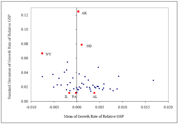
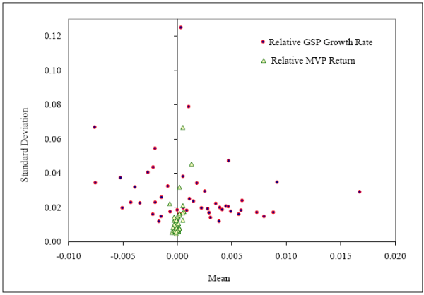
In addition to the adverse effects of behavioral biases, another set of factors that can influence state-level risk sharing is associated with the geographical location. Roughly speaking, investors who live in "riskier" regions would be more vulnerable to local economic shocks. For example, states like Alaska, North Dakota, and Wyoming have very volatile economies. As shown in Figure 4, the standard deviations of the state-specific component of their real per capita gross state product (GSP) growth rates are 0.125, 0.079, and 0.067, respectively. In contrast, states like Pennsylvania, Alabama, and Illinois, appear considerably less risky. The standard deviations of the state-specific component of their per capita GSP growth rate are only around 0.020.

To quantify the effects of geographical factors on risk sharing, for each state, we estimate the level of risk sharing that could be potentially attained if the investors in that state optimally use financial assets to minimize state-specific income risk. The theoretical state-level risk sharing measure characterizes the investment opportunities available to the investors in the state. Specifically, we use the relative gross state product to measure income before risk sharing, while the income after risk sharing is the return from a minimum variance composite portfolio that contains financial assets along with a state-specific "product" asset.³We choose financial assets from equity, bond, and treasury markets, and use the standard mean-variance optimization framework to identify the minimum variance portfolio (MVP) for each state. To measure the level of risk sharing that is potentially attainable, we use the Athanasoulis and Van Wincoop (2001) method and compare the volatility levels of the growth rate of relative GSP and the relative MVP return.⁴

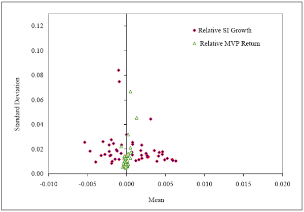
We examine the effects of behavioral and geographical factors on risk sharing using cross-sectional regressions in which the dependent variable is the level of risk sharing that is actually achieved by a U.S. state through the financial markets channel. We measure the achieved levels of risk sharing by comparing the volatility levels of the growth rate of relative GSP and relative state income (SI).⁵ The relative GSP reflects the state-specific component of income without smoothing from any risk sharing channel, while the relative SI captures the state-specific component of income that incorporates the smoothing effects of financial markets.

Our empirical investigation is organized around three key themes. First, to set the stage, we examine the influence of traditional factors such as the size and intensity of stock market participation and liquidity or borrowing constraints on state-level risk sharing.⁶ We find that, unconditionally, states with high stock market participation rates attain high levels of risk sharing. But when we account for borrowing constraints, as captured by the state-level housing collateral ratio (Lustig and Van Nieuwerburgh (2008)), surprisingly, higher levels of participation are associated with lower levels of risk sharing. Nonetheless, states with high participation rates achieve high levels of risk sharing when a greater proportion of aggregate state-level wealth is invested in the stock market. This evidence suggests that participation by wealthier investors, who might be relatively more sophisticated, improves state-level risk sharing.

The negative relation between stock market participation and risk sharing suggests that either the investment objectives of U.S. investors are not aligned with their risk sharing objectives or that their sub-optimal investment decisions generate low levels of risk sharing. In our second set of tests, we explicitly examine the effects of behavioral factors on state-level risk sharing. We find that the risk sharing levels are higher in states in which the cognitive abilities of investors are higher. Investors in high risk-sharing states also trade less frequently, exhibit a lower propensity to follow gambling-motivated strategies, exhibit a greater propensity to hold foreign stocks, and hold less concentrated portfolios.

Surprisingly, states in which investors tilt their portfolios disproportionately more toward local stocks also achieve higher levels of risk sharing. This result is inconsistent with the conjecture in Athanasoulis and Van Wincoop (2001). However, the evidence is consistent with the recent evidence from the retail investor literature, which demonstrates that the preference for local stocks could be induced by investors' superior local information and could reflect investor sophistication (e.g., Ivkovi ${\'{c\/}}$ and Weisbenner (2005), Massa and Simonov (2006), Bodnaruk (2008)). Overall, these results indicate that what matters for risk sharing is sophisticated stock market participation, where investors either follow the normative prescriptions of portfolio choice or attempt to exploit their superior private information.

In our last set of tests, we examine the effects of geographical factors on risk sharing. We present a novel approach to quantify the potential risk sharing opportunities available to investors in a state and examine whether the potential risk sharing levels are correlated with the achieved levels of risk sharing. Our evidence indicates that states can achieve higher levels of risk sharing when the risk sharing potential is high and state investors exhibit greater financial sophistication. We also find that high levels of sophistication does not improve risk sharing when potential risk sharing opportunities are low, which indicates that geographical location is an important determinant of risk sharing.

When we compare the effects of traditional, behavioral, and geographical factors on state-level risk sharing, we find that the behavioral effects are the strongest. These results are robust and cannot be explained by potential endogeneity of our sophistication measures, heterogeneity in industry composition (e.g., agriculture, mining, or manufacturing based state economy), size of the state economy, variation in people's age across states, regional differences in risk sharing, or the anomalous behavior of a handful of states.

The rest of the paper is organized as follows. In the next section, we present the risk-sharing estimates for individual U.S. states. In Sections 3 to 5, we present our main empirical results, where we examine the influence of traditional, behavioral, and geographical factors on state-level risk sharing, respectively. We present robustness test results in Section 6 and conclude in Section 7 with a brief discussion. Additional details about the data sources and estimation methods are presented in a detailed appendix.

2. State-Level Risk Sharing Estimates

2.1 Risk Sharing: The Basic Idea

In our paper, risk sharing refers to state-level income smoothing using financial markets. The income of a U.S. state is the sum of its output and the additional income it receives from various other sources. The output or the product of a state would be influenced by idiosyncratic shocks, but state income can be insulated from those output fluctuations through indirect channels such as financial markets. In an ideal scenario, U.S. states could reduce income risk by directly trading claims on state income in macro-markets (e.g., Shiller (1993), Shiller (2003)). But in the absence of directly traded claims on state income, an indirect mechanism like financial markets is an important income smoothing device available to a state. If a state utilizes financial assets effectively, the variance of the growth rate of state income would be lower than the variance of the growth rate of its output. We compare these two variances to quantify the level of income smoothing or risk-sharing in a state.

2.2 Risk Sharing Estimation Method

We use the Athanasoulis and Van Wincoop (2001) (hereafter AVW) methodology to estimate the level of risk sharing that can be achieved using financial assets.⁷ As in AVW, we focus on idiosyncratic (or state-specific) income risk. AVW quantify the level of risk sharing that can be attributed to financial markets by comparing the riskiness or the standard deviations of the growth rates of the relative gross state product (GSP) and relative state income (SI).⁸

The relative growth rates of the GSP and the SI for each state between years and are computed using the following growth rate differential:

$\displaystyle g_{i,t,t+1}^{rel}=g_{i,t,t+1}-g_{t,t+1}$ . $\displaystyle %$

(1)

Here, $g_{i,t,t+1}$ is the per capita growth rate of either the GSP or the SI of state

between years

and

, while $g_{t,t+1}$ is the per capita growth rate of either the U.S. GDP or the aggregate U.S. income.⁹ The relative GSP provides a measure of idiosyncratic or state-specific income growth rate before risk sharing, while relative SI reflects the state-specific income growth rate after risk sharing.

We also define a residual growth rate measure, which represents the unexpected or the unpredictable component of the corresponding raw growth rate measure. Specifically, we estimate the following regression to measure the residual growth rates of relative GSP and relative SI for state :

$\displaystyle g_{i,t,t+1}^{rel}=z_{i,t}\lambda+u_{i,t,t+1}$ . $\displaystyle % %$

(2)

Here, $z_{i,t}$ is a set of control variables for state

defined at time

and $u_{i,t,t+1}$ is the residual growth rate for state

defined over the interval between years

and

. $\lambda$ is a vector of coefficient estimates.¹⁰ Motivated by the results in Barro and Sala-i-Martin (1991, 1992) and Athanasoulis and Van Wincoop (2001), our set of control variables includes the lagged value of the relative GSP (or SI) growth rate, the logarithm of the initial per-capita GSP (or SI), and the five-year lagged population growth rate for the state.¹¹

Last, we use these growth rate measures to obtain the risk sharing (RS) estimate:

$\displaystyle RS=1-\frac{\sigma_{gRS}}{\sigma_{g}}$ . $\displaystyle %$

(3)

Here, $\sigma_{g}$ and $\sigma_{gRS}$ are the standard deviations of the income growth before risk sharing and after risk sharing, respectively. The RS measure takes two forms. The unconditional RS measure compares the standard deviations of the growth rates of relative GSP and relative SI. The conditional RS measure compares the standard deviations of the residual growth rates of relative GSP and relative SI obtained using equation (2).

Theoretically, the RS measure must lie between zero and one. Under full risk sharing, income risk is completely eliminated, $\sigma_{gRS}$ is zero, and the RS measure equals one. And in the absence of any risk sharing, there is no reduction in the income risk, $\sigma_{gRS}$ is equal to $\sigma_{g}$ , and the RS measure equals zero. In practice, however, the RS measure could be negative due to measurement error in the state-level income data.¹²

2.3 Income Data and Summary Statistics

We use inflation adjusted growth rates of per capita GSP and SI to calculate income growth rates before and after risk sharing.¹³ The gross domestic product (GDP) deflator obtained from the Bureau of Economic Analysis (BEA) is used to measure inflation. The state-level population data are from the Current Population Survey (CPS). The annual U.S. GDP and the GSP for individual states are also from the BEA. These data are available for the 1963 to 2004 period. The state income data are not provided by the BEA and they are available only for the 1963 to 1999 period.

Table 1, Panel A reports the summary statistics for various annual income growth rate measures. The mean growth rates of GDP and GSP are comparable (2.2% and 2.3%, respectively). But the average standard deviation of the GSP growth rate (= 3.7%) is considerably higher than the standard deviation of the GDP growth rate (= 2.0%). This evidence suggests that there exists considerable scope for improving risk sharing across the U.S. states. We also find that the standard deviations of SI and relative SI are lower than the standard deviations of GSP and relative GSP, respectively. These estimates indicate that financial assets are able to facilitate state-level risk sharing.

Examining the correlations among the growth rate measures, we find that there is considerable heterogeneity in the income growth rates across the U.S. states. The mean correlation between the GDP and the GSP growth rates is 0.509, while the mean correlation between the GDP and the SI growth rates is 0.551. The mean correlations between GSP and SI are also positive and above 0.70, but the estimates are not extremely high. These correlation estimates indicate that the level of risk sharing across the U.S. states is likely to exhibit considerable cross-sectional heterogeneity.

Figure 1: State-level unconditional risk sharing estimates (Time period: 1963-1999).

Figure 1 Data

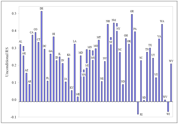
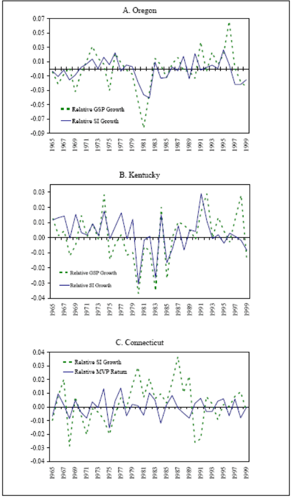
Figure 2: Panels A and B provide examples of income smoothing in a high and a low risk sharing state, respectively. In Panel C, for an arbitrarily chosen state, we illustrate the level of smoothing that can be potentially attained using financial assets.

Figure 2. Refer to link for figure data.

Figure 2 Data

2.4 Risk Sharing Estimates for Individual U.S. States

To better illustrate the observed heterogeneity in the state-level risk sharing measures, we use the income growth data and obtain conditional and unconditional risk sharing estimates for individual U.S. states. But first, in Table 2, Panel A, we report the aggregate level of risk sharing across all U.S. states.¹⁴ Our aggregate unconditional RS estimate of 26% and the aggregate conditional RS estimate of 23% measured over the 1963 to 1999 period are very similar to the AVW estimates obtained for the 1963 to 1999 period.

In Panel B of Table 2, we report the RS estimates for the individual U.S. states. For easier visualization, we also plot these results in Figure 1. The graphical evidence indicates that there is a rich cross-sectional variation in the state-level estimates of risk sharing. States like South Dakota (RS ) and Vermont (RS ) achieve very low levels of risk sharing, while states like California (RS = 0.39) and New York (RS 0.45) are able to substantially reduce their exposures to idiosyncratic income risk.

When we examine the time-series of the GSP and the SI growth rates for individual states, the income smoothing effect is evident more clearly. In Figure 2, Panels A and B, we plot the GSP and SI growth rates for a state with a very high level of risk sharing (Oregon) and a state with a very low level of risk sharing (Kentucky). These time series plots indicate that the ability of states to smooth income using financial assets varies significantly across the two risk sharing extremes.

The heterogeneity in a state's ability to engage in risk sharing estimates raises the natural question: What factors can explain these cross-sectional differences? In the rest of the paper, we identify the key determinants of the cross-sectional variation in risk sharing by examining the effects of traditional, behavioral, and geographical factors.

3. Traditional Determinants of Risk Sharing

In our first set of formal tests, we examine whether traditional factors such as the size of stock market participation and borrowing or credit constraints influence the ability of individuals to engage in risk sharing. We also examine whether the industry composition of a state influences its risk sharing ability. While previous studies conjecture that these traditional factors could determine the aggregate RS levels, we provide new results on the cross-sectional relation between the traditional factors and the state-level risk sharing.

3.1 Risk Sharing Regression Model

Our empirical analysis mainly focuses on state-level, cross-sectional risk sharing regressions. In these regressions, the dependent variable is either the unconditional or the conditional risk sharing measure (see Table 2, Panel B). The set of independent variable varies and depends upon the specific hypothesis to be tested. Table 3 reports the basic statistics and correlations for the main variables used in the empirical analysis.

We estimate the cross-sectional regressions using ordinary least squares (OLS) and correct the standard errors for heteroskedasticity. In particular, we estimate the following regression:

$\displaystyle y_{i}-\overline{y}=\left( x_{i}-\overline{x}\right) \beta+\varepsilon _{i}$ . $\displaystyle %$

(4)

In this equation, $y_{i}$ is either the unconditional or conditional RS measure for state

and $\overline{y}$ is the cross-sectional average of the state-level RS measures. $x_{i}$ is a vector of explanatory variables and $\overline{x}$ is the cross-sectional average vector corresponding to $x_{i}$ . $\beta$ is the vector of slope coefficient estimates. The random variable $\varepsilon_{i}$ is a zero-mean error term, which is assumed to be independent across states. Its variance is $\sigma_{i}^{2}$ , which differs across the U.S. states. We assume that $\varepsilon_{i}$ is heteroskedastic to ensure that our inference is not contaminated by unobserved state-specific shocks that are absorbed by the error term.

The dependent variable in our risk sharing regression is a generated variable that depends on the second moments of income growth rates. It is, therefore, measured with error. Fortunately, potential measurement error in the dependent variable does not result in inconsistent or biased OLS estimates (Green (2003), Chapter 5.6).

Both the dependent and independent variables in equation (4) are mean-free and, thus, our regression results do not include the estimates for the intercept.¹⁵ To allow for comparisons of coefficient estimates within and across regression specifications, we standardize both the dependent and the independent variables (mean is set to zero and the standard deviation is one). We also ensure that multi-collinearity does not affect our estimates.

Since we have only 51 state-level observations (including Washington DC), we try to develop parsimonious regression specifications by creating indices that combine multiple variables. Particularly, we define a sophistication index to capture the combined effects of all behavioral and cognitive abilities proxies.

3.2 Effect of Greater Stock Market Participation

If financial assets have the potential to facilitate risk sharing, one of the main reasons why some states achieve low levels of risk sharing might be related to the limited stock market participation rate in the state. To examine the relation between the state-level market participation rate and risk sharing, we consider a stock market participation proxy. Specifically, following Brown, Ivkovi ${\'{c\/}}$ , Smith, and Weisbenner (2008), we use an annual IRS data set for the 1998 to 2005 period, which reports the percentage of tax returns in each state that contains dividend income. We compute the average of this percentage over the 1998 to 2005 period and use it as a proxy for the state-level stock market participation rate.

The estimation results are reported in Table 4, Panel A. In the univariate specification, we find that there is a positive but insignificant relation between state-level RS and stock market participation (see columns (1) and (2)). For example, when we use the unconditional RS as the dependent variable, the estimate on the stock market participation proxy is 0.11 and its t-statistic is only 0.97. Although this coefficient estimate is not statistically significant, the evidence suggests that high market participation levels might be associated with high levels of risk sharing.

3.3 Do Weaker Borrowing Constraints Improve Risk Sharing?

To ensure that the stock market participation proxy is not simply capturing the ability of some investors to finance their investments through borrowing, we introduce a proxy for borrowing constraints in the risk sharing regression specification. We measure the severity of borrowing or liquidity constraints using the housing collateral ratio (HY) proposed in Lustig and Van Nieuwerburgh (2008). The state-level HY variable is defined as the ratio of state-level housing wealth, which can serve as collateral for loans, to the state-level human wealth. We summarize the method used to estimate the state-level HY in Section A.2 of the appendix.

We calculate the HY time-series for each state and use its time-series average in the risk sharing regressions. The regression results indicate that when HY is the only independent variable in the regression specification, it has a significantly positive coefficient estimate (see columns (3) and (4)). This evidence is consistent with the evidence in Lustig and Van Nieuwerburgh (2008), who use data for U.S. metropolitan areas to demonstrate that borrowing constraints affect risk sharing.¹⁶ Our finding that state-level HY can also explain the cross-sectional variation in state-level RS is new, although it is not totally surprising.

3.4 Does the Size and Intensity of Market Participation Matter?

To better understand the relative roles of market participation and borrowing constraints, we investigate whether the relative size of participation influences state-level risk sharing. We measure the relative size of a state's stock market exposure using the ratio of the state-level stock market wealth and the aggregate U.S. stock market wealth (Wealth Ratio).¹⁷ The wealth ratio for a state is computed using the state-level stock market wealth series from Case, Shiller and Quigley (2001). We use the wealth ratio as a rough proxy for the sophistication level of market participants, under the assumption that sophisticated investors would allocate a larger proportion of their wealth to financial assets.

The estimation results are reported in Table 4, Panel A (columns (5) and (6)). We find that there is a positive and statistically significant relation between the relative size of participation (i.e., the wealth ratio) and the state-level RS. However, the significance of this variable weakens in the presence of HY (see columns (7) and (8)). Somewhat surprisingly, we find that the coefficient estimate for the stock market participation proxy turns negative, although its estimate is statistically insignificant.

We further quantify the importance of stock market participation for state-level risk sharing by focusing on the intensity of stock market participation. We create a high participation dummy variable that is set to one for states in which the participation rate is above the median. The regression estimates with the high stock market participation dummy are reported in Table 4, Panel B.

The results in columns (1) and (2) indicate that the high participation dummy has a positive but statistically insignificant coefficient estimate. However, when we interact the high participation dummy with the wealth ratio variable, we find that the interaction term has a positive and statistically significant coefficient estimate. In particular, the estimation results reported in columns (3) and (4) indicate that the interaction term remains significant even in the presence of HY. The more parsimonious specifications in columns (5) to (8) yield very similar and somewhat stronger results.

This evidence suggests that risk sharing levels are higher in states in which investors allocate a larger proportion of their total wealth to stock investments, perhaps due to their greater financial sophistication. Interestingly, when we account for the effects of HY and relative wealth-high participation interaction, the market participation proxy has a significantly negative estimate. Thus, in the presence of a rough sophistication proxy, the coefficient estimate of the stock market participation variable is likely to reflect the adverse effects of unsophisticated participation.

Examining the economic significance of the estimates of the traditional factors, we find that HY has the strongest influence on state-level risk sharing. For instance, in column (5) of Panel B, the coefficient estimate of HY is 0.39. In economic terms, this estimate indicates that when the borrowing constraints weaken by one standard deviation, the risk sharing level increases by 0.39 standard deviation or $0.39\ast0.14=0.055.$ Relative to the mean state-level risk sharing estimate of 0.26 (see Table 3, row 1), there is a 20.22% increase in the level of risk sharing. The new RS level is 0.32, which reflects an economically significant jump in the level of RS.

3.5 Industry Differences Across States

Last, we examine the possibility that the heterogeneity in state-level risk sharing estimates reflect differences in industry composition across states. It is likely that states such as California and New York with more diversified economies would be able to withstand income shocks better than states with more concentrated economies (e.g., the Dakotas or Alaska). Certain industries such as agriculture and manufacturing are more sensitive to local economic shocks (Asdrubali, Sorensen and Yosha (1996)) than industries such as mining. Alternatively, states with greater ability for risk sharing would achieve greater industrial specialization and could have a more concentrated economy (Kalemli-Ozcan, Sorensen, and Yosha (2003)).

We examine the potential link between industry composition and risk sharing following the Asdrubali, Sorensen and Yosha (1996) approach. Specifically, we examine whether the GSP weights of the agricultural, mining and manufacturing sectors are related to the level of income risk sharing in a state. These specific industries are also used in Kalemli-Ozcan, Sorensen and Yosha (2003), who examine the determinants of regional specialization. In addition, we measure the industry concentration of each state using a Herfindahl index. Using data for the 1966 to 1997 period, for each state, we compute the proportion of GSP that a state derives from ten broad industry categories.¹⁸ We use these industry weights to compute the state-level Herfindahl index.

When we consider only the industry concentration measure in the regression specification, it has a positive but insignificant coefficient estimate (see Table 4, Panel C, columns (1) and (2)). This evidence indicates that differences in industry concentration could influence the level of risk sharing.¹⁹ When we include the three industry weights in the risk sharing regression specification, consistent with the previous evidence, we find that states with an agriculture-based economies have lower levels of risk sharing (see columns (3) and (4)). However, when we include the stock market participation, stock market wealth ratio, and the HY measures in the regression specification, neither of the industry measures is significant. This evidence indicates that the relation between industry composition and risk sharing is likely to reflect the heterogeneity in stock market participation rates, stock market wealth, and borrowing constraints (as captured by HY) across the states.

Collectively, the results summarized in Table 4 indicate that higher stock market participation rates are not sufficient to improve state-level risk sharing. The negative relation between participation and risk sharing suggests that either the investment objectives of U.S. investors are improperly aligned with the goal of risk sharing or that stock market participants' sub-optimal investment decisions lead to low levels of risk sharing.²⁰ This evidence is consistent with our conjecture that what is really needed for improving state-level risk sharing is sophisticated participation, where individuals invest broadly and significantly in the stock market.

4. Behavioral Biases and Risk Sharing

In our second set of tests, we examine whether frictions induced by investors' behavioral biases prevent U.S. states from achieving high levels of risk sharing.

4.1 Main Testable Hypotheses

We attempt to characterize the relation between the cognitive abilities and behavioral biases of individual investors and state-level risk sharing using two distinct hypotheses. The first hypothesis focuses on the direct relation between behavioral biases and state-level risk sharing. Specifically, we posit that:

Hypothesis 1: Risk sharing levels are higher in states in which investors have higher cognitive abilities, exhibit weaker behavioral biases, and possess greater overall financial sophistication.

In our second hypothesis, we examine whether behavioral biases also influence the relation between geographical location and the achieved levels of risk sharing.

Hypothesis 2: Risk sharing opportunities vary geographically across the U.S. states but higher state-level risk sharing opportunities can be exploited only when state investors are financially sophisticated.

We test the first hypothesis in the current section and provide empirical results to support the second hypothesis in Section 5.

4.2 Positive Effects of Cognitive Abilities

We begin by investigating whether higher levels of cognitive abilities of state investors are associated with higher levels of state-level risk sharing. This test is motivated by recent research in behavioral economics (e.g., Frederick (2005), Benjamin, Brown, and Shapiro (2006), Dohmen, Falk, Huffman, and Sunde (2007)), which finds that lower levels of cognitive abilities are associated with more "anomalous" preferences (e.g., greater level of impatience and stronger short-stakes risk aversion) and stronger behavioral biases. If investors' cognitive abilities are negatively associated with their behavioral biases, the investment decisions of low ability investors might not be aligned with the goal of minimizing total risk, which could in turn induce low levels of risk sharing.

Since it is extremely difficult to obtain direct measures of the cognitive abilities of stock market participants within each of the U.S. states, we adopt the imputation procedure to obtain state-level estimates of investors' cognitive abilities. Specifically, we use the empirical model of cognitive abilities (CAB) estimated in Korniotis and Kumar (2008). The dependent variable in the model is a direct measure of cognitive abilities (the average of verbal, quantitative and memory test scores) and a group of demographic variables, which have been identified by the psychology literature as the key correlates of cognitive abilities, are the independent variables. The empirical model indicates that investors with higher cognitive abilities are younger, wealthier, more educated, and more socially connected.²¹

We use the demographic characteristics of a sample of brokerage investors distributed across the U.S. to obtain the imputed CAB for all investors in that sample.²²The state-level CAB estimate is the equal-weighted average of imputed CAB estimates of all brokerage investors located in a state.²³ In our sample, investors in states like Kansas, Colorado, Missouri, Virginia, and Connecticut have high CAB estimates, while investors in states such as Arkansas, Maine, New Mexico, Florida, and South Carolina have low imputed CAB.

We do not use the state-level Census data directly to obtain imputed cognitive abilities for individual states because the Census data provide the characteristics of both market participants and non-participants. Direct measures of state-level IQ have a similar disadvantage. Because we want to quantify the CAB of only the market participants, the use of brokerage data seems most appropriate.

We re-estimate several specifications of the risk sharing regression after adding the state-level CAB measure to the set of the independent variables, which also contains the traditional determinants of state-level risk sharing. The estimation results are reported in Table 5 (columns (1) to (4)). In univariate specifications, we find that states with high cognitive ability investors achieve high levels of risk sharing. For example, in column (2), the coefficient estimate of CAB is 0.25 and its t-statistic is 2.24. Even when we include the stock market participation proxy, the HY, and the wealth ratio-high participation interaction term in the regression specification, the relation between cognitive abilities and risk sharing remains strong (estimate = 0.25, t-statistic = 2.77).²⁴

Consistent with our first hypothesis, these results indicate that the investment decisions of investors with higher cognitive abilities are more closely aligned with the goal of risk reduction, which eventually lead to higher levels of risk sharing. Since we use imputed values of investors' cognitive abilities instead of direct measures of their cognitive abilities, a more conservative interpretation of these findings is that states in which investors are younger, wealthier, better educated, and more strongly socially connected achieve higher levels of risk sharing, perhaps due to their weaker behavioral biases.

4.3 Adverse Effects of Behavioral Biases

To gather additional support for the first hypothesis, we examine the quality of investment decisions of individual investors directly. Using the investment decisions of brokerage investors, we obtain state-level estimates for the main behavioral biases identified in the recent behavioral finance literature. Like the state-level cognitive abilities measure, we obtain the state-level estimates of behavioral biases by computing an equal-weighted average of the behavioral bias measures of all investors within the state.

Specifically, for each state, we obtain estimates for the average portfolio turnover (an overconfidence proxy), the average percentage of local owners divided by our state-level participation proxy (participation-adjusted local bias proxy)²⁵, the portfolio weights in foreign stocks (home bias or diversification preference proxy), proportion of all trades that are in stocks with lottery-type features (gambling or speculation proxy)²⁶, and the normalized portfolio variance, which is the ratio of portfolio variance and the average correlation of stocks in the portfolio (portfolio concentration proxy).²⁷ We also consider the state-level cognitive abilities proxy. Together, these measures capture investor sophistication and serve as proxies for various behavioral biases such as overconfidence (e.g., Odean (1999), Barber and Odean (2000)), local bias (e.g., Huberman (2001), Grinblatt and Keloharju (2001), Ivkovic and Weisbenner (2005), Massa and Simonov (2006)), home bias (e.g., Lewis (1999)), gambling or speculation (e.g., Kumar (2008)), and under-diversification (e.g., Barber and Odean (2000), Goetzmann and Kumar (2008)).

As before, we estimate the risk sharing regressions using either the unconditional or the conditional RS measure as the dependent variable. The set of independent variables contain the behavioral bias proxies, the cognitive abilities proxy, and several control variables, including the traditional determinants of risk sharing. The results are presented in Table 5 (columns (5) to (8)).

The evidence indicates that risk sharing levels are higher when investors follow the normative prescriptions of portfolio theory. Across all specifications, we find that states in which investors do not trade very actively and hold relatively better diversified portfolios (i.e., hold less concentrated portfolios and include foreign stocks) achieve higher levels of risk sharing. In addition, the significantly positive coefficient of the cognitive abilities proxy remains significant in these specifications.

We also find that the estimates for the lottery preference proxy are negative, although their statistical significance is weak. This evidence indicates that a strong preference for speculative stocks that provide cheap bets but are risky is likely to reduce the level of risk sharing.

Interestingly, a stronger preference for local stocks is associated with higher levels of risk sharing. This finding is consistent with the recent evidence from the local bias literature, which supports the conjecture that local bias is induced by better information about local firms rather than pure familiarity (e.g., Ivkovi ${\'{c\/}}$ and Weisbenner (2005), Massa and Simonov (2006)). Because high local bias is associated with superior performance, the local bias measure can also be interpreted as another proxy for investor sophistication, which we find to be positively related to risk sharing.

Taken together, the regression results in Table 5 provide strong support for our first hypothesis. They indicate that the sensitivity to state-specific income shocks is reduced considerably when investors within a state follow the normative prescriptions of portfolio theory. Somewhat surprisingly, we also find that informed deviations from the normative prescriptions of portfolio theory (i.e., information-induced local bias) facilitate risk sharing.

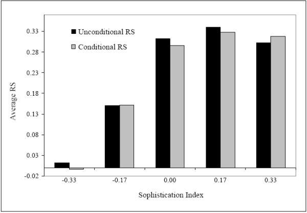
4.4 Quantifying the Behavioral Effects Using a Sophistication Index

In this section, we attempt to quantify the combined effects of all behavioral bias and cognitive abilities proxies on risk sharing. We also investigate whether the behavioral effects are stronger than the traditional determinants of risk sharing (i.e., market participation rate, size of participation, and borrowing constraints). Because we have a limited number of state-level observations (only 51), we aggregate the behavioral bias and cognitive abilities proxies into one composite sophistication index and choose parsimonious risk sharing regression specifications.

Figure 3: Investor sophistication and state-level risk sharing.

Figure 3 Data

We construct the sophistication index as follows. First, for each behavioral bias proxy (e.g., portfolio turnover), we create a dummy variable. The dummy variable takes the value of one for states in which the bias proxy is above the $q^{th}$ percentile ( = 25, 50, or 75). We then add the dummy variables corresponding to the measures that are positively related to RS (cognitive ability, local preference, and percentage of foreign stock) and subtract the dummy variables for the measures that are negatively related to RS (portfolio turnover, portfolio concentration, and lottery preferences). The resulting total is divided by six. This linear combination of the behavioral bias proxies is our sophistication index. For robustness, we define a continuous sophistication index using standardized (mean = 0, std. dev. = 1) bias measures instead of the six behavioral bias dummy variables.

We also define an "unsophistication" index, which is computed just like the sophistication index. In this instance, however, the dummy variable associated with a behavioral bias proxy takes the value of one if the state-level bias proxy is below the $25^{th}$ percentile.

As expected, we find a positive relation between state-level investor sophistication and state-level risk sharing. This positive relation is evident in Figure 3. For = 75, the figure shows the average level of RS for the distinct values of the sophistication index. Consistent with our previous evidence, we find that among states with low levels of sophistication (index value = -0.33 or -0.17), the average RS is 0.121. But, for states with higher levels of sophistication (index $\geq$ 0), the average RS estimate is 0.308. In economic terms, a jump in the sophistication level of investors from the low to the high value of the sophistication index corresponds to a 154% increase in the level of risk sharing.

We also re-estimate the risk sharing regressions, where the sophistication index is the main independent variable and the traditional determinants of risk sharing serve as control variables. The estimation results reported in Table 6, Panel A show that the sophistication index is a significant determinant of risk sharing across all specifications. Further, the higher the value of , the higher is the estimate and the t-statistic for the sophistication index. The monotonic increase in the estimate and the t-statistic confirms our conjecture that states with the most sophisticated investors are able to reduce the sensitivity to state-specific idiosyncratic income risk most effectively. We find similar results with the continuous sophistication index.

When we compare the estimate for the sophistication index to the estimates for the traditional determinants of risk sharing, we find that the coefficient estimate of the sophistication index is comparable to the estimates of strong traditional factors such as HY. For instance, in column (6), the sophistication index has a coefficient estimate of 0.56 (t-statistic = 5.81) while HY has an estimate of 0.42 (t-statistic = 4.79). This evidence indicates that both traditional and behavioral factors are important determinants of state-level risk sharing.

4.5 State-Level Education: An Alternative Sophistication Proxy

For robustness, we consider the average education level of individuals in a state as an alternative proxy for investor sophistication. This variable is defined as the proportion of residents in a state with a Bachelor's or higher educational degree. The education data are obtained from the 1990 U.S. Census.

We find that the correlation between the education measure and our sophistication index is 0.40. This estimate indicates that our sophistication index estimated using the brokerage data is reasonable because it has the expected positive correlation with an aggregate state-level measure obtained from a completely different source.

We also re-estimate the risk sharing cross-sectional regressions with the education measure as an additional independent variable and report the results in Panel B of Table 6. We find that, like the estimates for the sophistication index, education has positive coefficient estimates. However, their statistical significance is weak (see columns (1)-(4)). For instance, in column (2), the education variable has a coefficient estimate of 0.18 and a t-statistic of 1.71. When we include both the sophistication index and the education variable in the regression specification, the sophistication index has a significantly positive coefficient estimate, while the estimates for education become statistically insignificant (see columns (5) and (6)).

These robustness check results indicate that our sophistication index, which captures the financial sophistication of only the stock market investors within a state, is more strongly associated with the state-level risk sharing than the education variable, which reflects the sophistication level of both market participants and non-participants. Nonetheless, the weakly positive estimate for education in the risk sharing regression is comforting. This evidence also highlights the strengths of the brokerage data set, which we use to measure the quality of investment decisions of individuals who choose to participate in the market.²⁸

Collectively, the risk sharing regression results with the behavioral bias proxies indicate that the levels of risk sharing are higher in states in which investors have higher cognitive abilities and exhibit weaker behavioral biases. Even when the size of market participation is large, lack of financial sophistication could hurt risk sharing. These findings provide strong empirical support for our first hypothesis and indicate that both traditional and behavioral factors are important determinants of state-level risk sharing.

Of course, these results should be interpreted with some degree of caution because the time-periods used to measure investors' level of financial sophistication and risk sharing do not fully overlap. The investment decision measures are estimated using data from 1991 to 1996, while the state-level risk sharing estimates are obtained for the 1963 to 1999 period. However, the evidence of a significant relation between the investor sophistication measures estimated using the retail brokerage data and the risk sharing measures estimated using state-level macro-economic data is quite remarkable. We suspect that the relation between risk sharing and investor sophistication would be stronger if more accurate measures of people's investment decisions using a longer panel on the stock-holdings and trades of U.S. households are employed in the analysis.

Figure 4: Mean and standard deviation of income before risk sharing.

Figure 4 Data

5. Does Geographical Location Influence Risk Sharing?

If some U.S. states are inherently riskier, in addition to the traditional and the behavioral factors, the geographical location could influence the magnitude of state-level risk sharing. The graphical evidence in Figure 4 indicates that the standard deviations of relative GSP growth rates for states like Alaska, North Dakota, and Wyoming are significantly higher than the standard deviations of relative GSP growth rates for Alabama, Illinois, and Pennsylvania. For riskier states, reducing the sensitivity to idiosyncratic state-specific income risk would be very difficult, unless the sophistication level of state investors is very high.

In this section, first, we quantify the extent to which geographical location determines the level of risk sharing opportunities that are available to investors within a state. Next, we investigate whether the geographical, behavioral, and traditional effects interact to generate the overall level of interstate risk sharing. Together, these empirical tests allow us to gather support for the second hypothesis.

5.1 Potential Risk Sharing Estimation Method

To quantify the role of location on risk sharing, for each state, we compute a state-specific theoretical benchmark. This benchmark reflects the potential risk sharing opportunities offered by financial markets to the individuals in that state. Thus, it quantifies the degree of difficulty that investors in a particular state might face when attempting to reduce their exposure to the idiosyncratic, state-specific income risk.

We compute the level of risk sharing that a U.S. state can potentially attain by minimizing the total variance of a composite portfolio that contains the "product asset" of the state (i.e., a perpetual claim to GSP) and a broad set of financial assets. As in Fama and Schwert (1977) and Jagannathan and Wang (1996), we assume that the return from the product asset is the growth rate of GSP.²⁹ We require the total return of the composite portfolio to be at least as high as the return from the state's income asset (i.e., the growth rate of SI).³⁰

Our potential risk sharing computation method adopts a general equilibrium approach. To ensure that the equilibrium returns of financial assets are not affected by the risk sharing induced trading strategies, we set the weight on the product asset to be equal to the ratio of GSP to the total state wealth. Further, we constrain the total weight on financial assets to be equal to the average ratio of the state financial wealth and the total state wealth.

Using the mean-variance optimization framework, for each state, we compute a set of portfolio weights that characterizes the minimum variance portfolio (MVP) of that state. To calculate the MVP weights, we use the GSP and the asset return data for the 1966 to 2004 period.³¹ The MVP weights allow us to obtain the return of the MVP portfolio ( $r_{pt}$ ), which reflects the income growth rate associated with the potential level of risk sharing. The state-specific income after risk sharing is the difference between $r_{pt}$ and the mean of $r_{pt}$ across all states in year . We denote the deviation of the $r_{pt}$ from its cross-sectional mean as relative MVP return.

To calculate the level of risk sharing that can be potentially attained, we use the risk sharing measure defined in equation (3), where we replace the standard deviation of growth rate of relative SI ( $\sigma_{SI}$ ) by the standard deviation of relative MVP return ( $\sigma_{MVP}$ ). As before, the state-specific income before risk sharing is the relative growth rate of GSP. Therefore, the denominator in the RS equation (= $\sigma_{g}$ ) remains unchanged.

Since we use all the available data to estimate one set of fixed weights for each state, the weights exploit all the in-sample variation in the GSP and financial asset returns. Thus, they should be interpreted as full information, ex-post weights. Similarly, the potential RS estimate should be viewed as a benchmark that captures the potential level of risk sharing under full information.³²

Figure 5: Mean and standard deviation of income before (relative GSP growth rate) and after (relative MVP return) potential level of risk sharing.

Figure 5 Data

Figure 6: Mean and standard deviation of income after achieved (relative SI growth rate) and potential (relative MVP return) levels of risk sharing.

Figure 6 Data

5.2 Potential Risk Sharing Estimates

The MVP computation requires a set of financial assets. For feasibility, we consider a set of broad stock market and debt indices that can effectively quantify the investment opportunities offered by financial markets. Our choice is based on the evidence from the existing literature, which shows that financial assets contain information about the state of the aggregate economy (e.g., Lamont (2001)). If economic activities across U.S. states are correlated, financial assets might also contain information about the income growth rates of individual states and could provide opportunities for risk reduction.

Specifically, our broad stock market indices include the monthly returns of the three Fama-French factors (Fama and French (1992, 1993)) and the momentum factor (Jegadeesh and Titman (1993), Carhart (1997)). The set of debt instruments include the monthly yields for the 30-day Treasury Bill and 10-year government bond. We also use the monthly yields for Aaa and Baa rated corporate bonds. In Section A.6 of the appendix, we discuss our choice of financial assets in considerable detail. Table 1, Panel B presents the basic summary statistics for all financial assets and their correlations with the income growth measures.

Figure 5 reports the mean and the standard deviation of income before and after potential level of risk sharing for all U.S. states. It is evident from the plot that financial assets have the potential to reduce the risk levels of product assets substantially. The average standard deviation can potentially be reduced from 0.0272 to 0.0121, which corresponds to a more than a 50% decline. Even riskier states like Alaska, North Dakota, and Wyoming have large opportunities for risk sharing using financial assets. For instance, in Alaska, financial assets can reduce the risk by almost one-third (from 0.125 to 0.067). Further, the mean estimates of the relative MVP return for all states are similar and closer to zero, which indicates that all states would grow at the national rate.³³

Table 7 reports the potential risk sharing estimates. In Panel A, we report the aggregate potential RS across all states. The aggregate potential RS estimate is 0.62, which is more than twice the aggregate level of RS that is actually achieved (= 0.26). Similarly, the potential RS for individual states reported in Panel B are always higher than the corresponding achieved RS levels (see Table 2, Panel B). For some states, the difference between the potential and the achieved RS levels is quite large. In particular, states like Nebraska, South Dakota and Vermont are able to achieve less than 15% risk sharing even though the potential RS estimates for those states are above 65%.

In sum, the state-level potential risk sharing estimates indicate that existing financial markets offer significant risk sharing opportunities. If investors exploit the available risk sharing potential, there would be a significant reduction in the level of standard deviation of the income growth rate. Comparing the potential risk sharing estimates with the actual levels of risk sharing, we find that although states are able to reduce the income risk, the potential for further improvement is significant (see Figure 6).

5.3 Potential versus Actual Levels of Risk Sharing

To understand why states with large risk sharing opportunities are unable to exploit them, we re-estimate risk sharing regressions with enhanced specifications. As before, in the regressions, the achieved RS level for a state is the dependent variable. The set of independent variables contains the potential level of RS, along with the traditional and the behavioral determinants of risk sharing.

The results are reported in Table 8. The estimation results indicate that the potential RS is not a significant predictor of achieved RS. Specifically, in columns (1) and (2), the coefficient estimates for potential RS are 0.10 (t-statistic = 0.72) and 0.00, (t-statistic = 0.01), respectively.³⁴ This evidence indicates that the investment decisions of state investors might not be aligned with the goal of improving risk sharing.

To further examine the relation between the potential and the achieved levels of risk sharing, we replace the potential RS variable in the risk sharing regression with a high potential RS dummy variable. The dummy variable takes the value of one if a state's potential RS estimate is above the median, and zero otherwise. It tests whether investors exploit risk sharing opportunities and achieve high levels of RS when the potential RS level is high.³⁵ The results in columns (3) and (4) indicate that when the potential risk sharing opportunities are high, the achieved RS levels are also high.³⁶

Next, we formally test our second hypothesis, which posits that high risk sharing opportunities are more (less) effectively exploited when the level of investor sophistication is high (low). We define two interaction terms to test the hypothesis. First, we interact the sophistication index with the high potential RS (above median) dummy variable. Second, we interact the sophistication index with a low potential RS (below the 25th percentile) dummy variable. If sophisticated investors are better able to exploit the high risk sharing opportunities offered by financial markets, then the first interaction term would be positively correlated with the achieved levels of RS, while the second interaction term would either be uncorrelated or negatively correlated with the achieved RS variable.

We estimate the risk sharing regressions after including the two interaction terms in the set of independent variables and report the estimates in Table 8 (columns (5) to (8)). Consistent with our conjecture, we find that the sophistication-high potential RS interaction term has a positive and statistically significant estimate (see columns (5) and (6)). In addition, the sophistication-low potential RS interaction term has a negative coefficient estimate, although it is statistically significant in the conditional risk sharing regression (see columns (7) and (8)). This evidence indicates that even high levels of financial sophistication cannot improve risk sharing when the potential risk sharing opportunities are modest.

In sum, the state-level potential risk sharing estimates indicate that existing financial markets offer significant risk sharing opportunities. If investors exploit the available risk sharing potential effectively, there would be a significant reduction in the level of standard deviation of the income growth rate and even the mean of the income growth rate would be significantly higher.³⁷

6. Robustness Checks and Alternative Explanations

In this section, we carry out additional tests to entertain alternative explanations and examine the robustness of our results. We use specifications (5) and (6) from Table 8, which summarize the key results in our paper, and include additional control variables to examine the sensitivity and robustness of those main findings. The results from these additional tests are summarized in Table 9.

6.1 Size of the State Economy

In the first test, we examine whether the risk sharing levels are lower in smaller (i.e., lower GSP) states that might have riskier economies. We use the state-level GSP at the beginning of the sample period as a proxy for the size of the state economy and include it in the risk sharing regression specification. The results indicate that larger states achieve higher levels of risk sharing, but the size-risk sharing relation is statistically very weak (see columns (1) and (2)).

6.2 Do Smarter Investors Move to High Risk Sharing States?

A potential concern with our baseline risk sharing regression specification is that the sophistication index might be endogenous. It is possible that sophisticated investors self-select into states in which risk sharing opportunities are higher and smoothing income shocks is relatively easier. To account for this potential endogeneity, in the second test, we estimate our baseline regressions using an instrumental variable (IV) estimator. We instrument the sophistication index with initial per capita GSP. We also instrument the interaction term between high potential risk sharing and sophistication with an interaction term between high potential risk sharing and initial GSP.

Initial GSP is a valid instrument for at least two reasons. First, because the initial GSP is measured in 1966 (the beginning of our sample period), it should be uncorrelated with the error term of the regression. Second, it is highly correlated with the sophistication index. In unreported results we find the correlation coefficient is 0.50.³⁸

The IV estimation results are presented in Table 9, columns (3) and (4). We find that the coefficient estimates for the sophistication index are 0.51 (-statistic = 3.08) and 0.56 (-statistic = 2.67) in the unconditional and conditional risk sharing regressions. These estimates are very similar to the OLS estimates reported in Table 8, column (5) (estimate = 0.53, -statistic = 4.76) and column (6) (estimate = 0.48, -statistic = 4.26). Further, much like the OLS results, the significance of the potential risk sharing-sophistication interaction term is lower than that of the non-interacted sophistication index. For example, when the dependent variable is the conditional risk sharing measure, the OLS estimate and -statistic are 0.20 and 2.10, respectively (Table 8, column (6)), while the IV estimate and -statistic are 0.47 and 1.74, respectively (Table 9, column (4)). These IV estimates indicate that our key results are unlikely to be induced by the potential endogeneity of the sophistication index.

6.3 Age Composition of the State

In the next test, we examine whether the age composition of the population in a state influences our results. For example, risk sharing levels could be high in states such as Florida with a large concentration of older investors just because those older investors have accumulated more financial assets over their lifetime.³⁹ But older investors might also make worse investment decisions (e.g., Korniotis and Kumar (2007)), which can reduce the level of risk sharing. When we include average age of the state population as an additional independent variable in the specification, we find that it has a statistically insignificant coefficient estimate (see columns (5) and (6)). Thus, age differences across states do not have an incremental ability to explain the cross-sectional variation in the level of risk sharing.

6.4 Regional Variation in Risk Sharing

In the fourth robustness test, we examine whether our results reflect the known regional variation in the level of risk sharing (e.g., Sorensen and Yosha (2000)). Using the regional classification scheme from the U.S. Census, we define three regional dummy variables and include them in the risk sharing regressions. We find that relative to the Southern states, the states in the West are able to achieve higher levels of risk sharing, while Mid-Western states have somewhat lower levels of risk sharing (see columns (7) and (8)). The North-East region dummy has negative coefficient estimates, but they are insignificant. More importantly, the inclusion of these regional dummy variables do not significant lower the statistical or the economic significance of the behavioral and geographical factors. Among the traditional factors, the HY variable is no longer significant, which indicates that the variation in state-level HY that matters for risk sharing is regional. This evidence is not surprising because there is a strong regional component in the real estate market. In untabulated results, consistent with this conjecture, we find that when we define HY at the regional level, it has a significant coefficient estimate (estimate = 0.23, t-statistic = 2.14).

6.5 Finite Sample Bias and the Effect of Outliers

Last, we conduct two randomization tests to ensure that our regression estimates are not influenced by the finite sample bias or the abnormal behavior of only a handful of states. First, we re-estimate the risk sharing regression (specification (6) from Table 8) after randomly excluding five states from the sample. We repeat the process 1,000 times and examine the distributions of the coefficient estimates of the independent variables considered in Table 8, column (6). In untabulated results, we find that the coefficient estimates from the randomized sub-samples are very similar to the full-sample estimates. Both the mean and the median estimates are almost identical to the estimates reported in Table 8, column (6). This evidence indicates that our results are not driven by outliers.

In the next randomization test, we create 2,500 bootstrapped samples by choosing states randomly with replacement. We find that, in most iterations, the coefficient estimates reported in Table 8 (column (6)) are higher in magnitude than the bootstrap estimates. Thus, we are able to reject the null hypothesis that the traditional, behavioral, and geographical factors are insignificant determinants of the cross-sectional variation in state-level risk sharing. The p-values corresponding to these independent variables are all below 0.08.

Taken together, the results from these additional tests indicate that our risk sharing regression estimates are robust. The main results cannot be fully explained by potential endogeneity of our sophistication measures, heterogeneity in the size of the state economy and people's age across states, regional differences in risk sharing, or the anomalous behavior of a handful of states.

7. Summary and Conclusion

This study presents the first comprehensive analysis of the determinants of state-level income risk sharing (or income smoothing). We focus on the aggregate effects of behavioral biases, but we also study the effects of traditional and geographical factors on the level of risk sharing across the U.S. states.

We present three key results. First, we show that merely high levels of stock market participation rates do not generate high levels of risk sharing. In fact, after accounting for borrowing constraints, on average, states in which individuals participate more in the stock market achieve low levels of risk sharing. The risk sharing levels are high when individuals invest broadly and significantly in the stock market, perhaps due to their greater financial sophistication.

Second, we show that risk sharing levels are higher in states in which investors trade less frequently, exhibit a lower propensity to follow gambling-motivated strategies, exhibit a greater propensity to hold foreign stocks, and hold less concentrated portfolios. In other words, investors who follow the normative prescriptions of portfolio theory facilitate risk sharing at the aggregate level. Surprisingly, risk sharing is also enhanced when investors deviate from the theoretical benchmarks and tilt their portfolios toward local stocks due to an informational advantage.

Third, we show that the potential to achieve high levels of risk sharing varies geographically across the U.S. states. However, the available opportunities for risk sharing are exploited effectively when investors within a state have higher levels of cognitive abilities and exhibit weaker behavioral biases. The geographical location is also important because even very sophisticated investors are unable to improve risk sharing when the potential risk sharing opportunities are modest. Collectively, our results indicate that the influence of investors' cognitive abilities and behavioral biases extend beyond the domain of financial markets to the aggregate macro-economy.

These empirical findings make several useful contributions. First, our study integrates three distinct and somewhat unconnected strands of literature on interstate risk sharing, the ability of financial assets to capture current and future economic activities, and the growing literature on household finance. We show that people's sub-optimal investment decisions aggregate up and the adverse effects of the associated biases can be detected even in the aggregate, state-level macro-economic data. Although we do not attempt to quantify the total welfare cost of these biases, unlike the evidence in Calvet, Campbell, and Sodini (2007), our results suggest that aggregate behavioral biases could adversely effect social welfare.

Beyond the contributions to the behavioral finance and the risk sharing literatures, our potential risk sharing estimates are useful because they provide a more precise characterization of the degree of market incompleteness, which in turn has important implications for asset pricing.⁴⁰ Because market incompleteness is a statement about the investment environment and is not necessarily related to the decisions of investors, the potential risk sharing estimates that only reflects the characteristics of the investment environment could provide a more accurate assessment of the degree of market incompleteness. Our results indicate that, at least from the perspective of interstate risk sharing, financial markets are more complete than previously believed, although they appear more incomplete due to people's sub-optimal investment decisions. In light of this evidence, consumption-based asset pricing models employed to investigate the implications of market incompleteness should be extended to account for investors' behavioral biases.

Our findings also have distinct policy implications. First, they indicate that state-level risk sharing would not improve by simply increasing stock market participation rates. Efforts to increase stock market participation should also attempt to increase sophisticated participation. In particular, improvements in financial literacy might be needed to improve state-level risk sharing. Second, since very high levels of income risk sharing can be potentially attained through the financial markets channel, federal policies should encourage the development of state-specific mutual funds. If used effectively, those funds could allow people to have smoother income stream, and hence smoother consumption, thereby improving social welfare. Thus, in broader terms, our results reinforce the notion that increased and sophisticated financial market participation can improve social welfare.

Bibliography

Amemiya, T., 1985

"Advanced Econometrics," Harvard University Press, Cambridge, Massachusetts.

Asdrubali, P., B. E. Sorensen, and O. Yosha, 1996

"Channels of Interstate Risk Sharing: United States 1963-1990," Quarterly Journal of Economics, 111, 1081-1110.

Athanasoulis, S. G., and E. Van Wincoop, 2001

"Risk Sharing Within the United States: What do Financial Markets and Fiscal Federalism Accomplish?," Review of Economics and Statistics, 83, 688-698.

Barber, B. M., and T. Odean, 2000

"Trading is Hazardous to Your Wealth: The Common Stock Investment Performance of Individual Investors," Journal of Finance, 55, 773-806.

Barber, B. M., and T. Odean, 2001

"Boys will be Boys: Gender, Overconfidence, and Common Stock Investment," Quarterly Journal of Economics, 116, 261-292.

Barber, B. M., T. Odean, and N. Zhu, 2008

" Do Noise Traders Move Markets?," Review of Financial Studies, Forthcoming.

Barberis, N., and M. Huang, 2008

" Stocks as Lotteries: The Implications of Probability Weightings for Security Prices," American Economic Review, Forthcoming.

Barberis, N., M. Huang, and T. Santos, 2001

" Prospect Theory and Asset Prices," Quarterly Journal of Economics, 116, 1-53.

Barberis, N., and R. Thaler "A Survey of Behavioral Finance," Handbook of the Economics of Finance, G. M. Constantinides, M. Harris, and R. M. Stulz, eds., Elsevier B.V., Amsterdam, Netherlands.

Barro, R. J., 1990

"The Stock Market and Investment," Review of Financial Studies, 3, 115-131.

Barro, R. J., and X. Sala-i-Martin, 1991

" Convergence Across States and Regions," Brookings Papers on Economic Activity, 1991, 107-182.

Barro, R. J., and X. Sala-i-Martin, 1992

" Convergence," Journal of Political Economy, 100, 223-251.

Baxter, M., and U. J. Jermann, 1997

"The International Diversification Puzzle Is Worse Than You Think," American Economic Review, 87, 170-180.

Benjamin, D. J., S. A. Brown, and J. M. Shapiro, 2006

"Who is `Behavioral'? Cognitive Ability and Anomalous Preferences," Working Paper (May), University of Chicago and Harvard University.

Benartzi, S., and R. Thaler "Myopic Loss Aversion and the Equity Premium Puzzle," Quarterly Journal of Economics, 110, 73-92.

Bernanke, B. S., and A. S. Blinder, 1992

"The Federal Funds Rate and the Channels of Monetary Transmission," American Economic Review, 82, 901-921.

Bodnaruk, Andriy, 2008

"Proximity Always Matters: Local Bias when the Set of Local Companies Changes," Working Paper (April), University of Notre Dame.

Bottazzi, L., P. Pesenti, and E. Van Wincoop, 1996

"Wages, Profits and the International Portfolio Puzzle," European Economic Review, 40, 219-254.

Brandt, M. W., J. H. Cochrane, and P. Santa-Clara, 2006

"International Risk Sharing is Better Than You Think, or Exchange Rates are Too High," Journal of Monetary Economics, 53, 671-698.

Brown, J. R., Z. Ivkovi ${\'{c\/}}$ , P. A. Smith, and S. Weisbenner, 2008 "Neighbors Matter: Causal Community Effects and Stock Market Participation," Journal of Finance, 63, 1509

-1531.

Browning, M., and S. Leth-Petersen, 2003

"Imputing Consumption From Income and Wealth Information," Economic Journal, 113, F282-301.

Calvet, L. E., J. Y. Campbell, and P. Sodini, 2007

"Down or out: Assessing the Welfare Costs of Household Investment Mistakes," Journal of Political Economy, 115, 707-747.

Campbell, J. Y., 1996

"Understanding Risk and Return," Journal of Political Economy, 104, 298-345.

Campbell, J. Y., 2006

"Household Finance," Journal of Finance, 61, 1553-1604.

Campbell, J. Y., and J. H. Cochrane, 1999

, "By Force of Habit: A Consumption-Based Explanation of Aggregate Stock Market Behavior," Journal of Political Economy, 107, 205-251.

Carhart, M., 1997

"On Persistence of Mutual Fund Performance," Journal of Finance, 52, 57-82.

Cochrane J., 1991

"A Simple Test of Consumption Insurance," Journal of Political Economy, 99, 957-976.

Constantinides, G. M., and D. Duffie, 1996

" Asset Pricing with Heterogeneous Consumers," Journal of Political Economy, 104, 219-240.

Coval, J. D., and T. Shumway, 2005

" Do Behavioral Biases Affect Prices?," Journal of Finance, 60, 1-34.

Crucini, M., 1999

"On International and National Dimensions of Risk Sharing," Review of Economics and Statistics, 81, 73-84.

Davis, S. J., and P. Willen, 2000

" Occupation-Level Income Shocks and Asset Returns: Covariance and Implications for Portfolio Choice," NBER Working Paper # 7905.

Davis, S. J., and P. Willen, 2000

"Using Financial Assets to Hedge Labor Income Risk: Estimating the Benefits," Working Paper (March), University of Chicago.

Davis, S. J., and P. Willen, 2002

"Risky Labor Income and Portfolio Choice," Innovations for Financing Retirement, Z. Bodie, O. S. Mitchell, B. Hammond, and S. Zeldes, eds., University of Pennsylvania Press.

Dohmen, T., A. Falk, D. Huffman, and U. Sunde, 2007

"Are Risk Aversion and Impatience Related to Cognitive Ability?," IZA Discussion Paper No. 2735.

Fama, E. F., and G. W. Schwert, 1977

"Human Capital and Capital Market Equilibrium," Journal of Financial Economics, 4, 95-125.

Fama, E. F., and K. R. French, 1992

"The Cross-Section of Expected Returns," Journal of Finance, 47, 427-456.

Fama, E. F., and K. R. French, 1993

"Common Risk Factors in the Returns on Stocks and Bonds," Journal of Financial Economics, 33, 3-56.

Frederick, S., 2005

"Cognitive Reflection and Decision Making," Journal of Economic Perspectives, 19, 25-42.

Friedman, B. M., and K. N. Kuttner, 1992

" Money, Income, Prices, and Interest Rates," American Economic Review, 82, 472-492.

Gertler, M., and C. S. Lown, 1999

"The Information in the High Yield Bond Spread for the Business Cycle: Evidence and Some Implications," Oxford Review of Economic Policy, 15, 132-150.

Graham, J. R., and A. Kumar, 2006

"Do Dividend Clienteles Exist? Evidence on Dividend Preferences of Retail Investors," Journal of Finance, 61, 1305-1336.

Graham, J. R., C. R. Harvey, and H. Huang, 2006

"Investor Competence, Trading frequency, and Home Bias," Working Paper (May), Fuqua School of Business, Duke University.

Greene, W. H., 2003

Econometric Analysis, 5th Edition, Prentice Hall, New Jersey.

Grinblatt, M., and B. Han, 2005

" Prospect Theory, Mental Accounting, and Momentum," Journal of Financial Economics, 78, 311-339.

Grinblatt, M., and M. Keloharju, 2001

"What Makes Investors Trade?" Journal of Finance, 56, 589-616.

Harvey, C. R., 1988

"The Real Term Structure and Consumption Growth," Journal of Financial Economics, 22, 305-333.

Harvey, C. R., 1989

"Forecasts of Economic Growth from the Bond and Stock Markets," Financial Analysts Journal, 45, 38-45.

Hess, G. D., and K. Shin, 2000

"Risk Sharing by Households Within and Across Regions and Industries," Journal of Monetary Economics, 45, 533-560.

Hirshleifer, D., 2001

"Investor Psychology and Asset Prices" Journal of Finance, 56, 1533-1597.

Huberman, G., 2001

"Familiarity Breeds Investment," Review of Financial Studies, 14, 659-680.

Ivkovi ${\'{c\/}}$ , Z., J. Poterba, and S. Weisbenner, 2005

"Tax-Motivated Trading by Individual Investors," American Economic Review, 95, 1605-1630.

Ivkovi ${\'{c\/}}$ , Z., C. Sialm, and S. Weisbenner, 2008

"Portfolio Concentration and the Performance of Individual Investors," Journal of Financial and Quantitative Analysis, Forthcoming.

Ivkovi ${\'{c\/}}$ , Z., and S. Weisbenner, 2005

"Local Does as Local Is: Information Content of the Geography of Individual Investors' Common Stock Investments," Journal of Finance, 60, 267-306.

Jacobs, K., and K. Wang, 2004

"Idiosyncratic Consumption Risk and the Cross Section of Asset Returns," Journal of Finance, 59, 2211-2252.

Jagannathan, R., and Z. Wang, 1996

"The Conditional CAPM and the Cross-Section of Expected Returns," Journal of Finance, 51, 3-53.

Jagannathan, R., and T. Ma, 2003

"Risk Reduction in Large Portfolios: Why Imposing the Wrong Constraints Helps," Journal of Finance, 58, 1651-1684.

Jegadeesh, N., and S. Titman, 1993

"Returns to Buying Winners and Selling Losers: Implications for Stock Market Efficiency," Journal of Finance, 48, 65-91.

Kalemli-Ozcan, S., B. E. Sorensen, and O. Yosha, 2003

"Risk Sharing and Industrial Specialization: Regional and International Evidence," American Economic Review, 93, 903-918.

Kanazawa, S., 2006

"IQ and the Wealth of States," Intelligence, 34, 593-600.

Kashyap, A. K., J. C. Stein, and D. W. Wilcox, 1993

"Monetary Policy and Credit Conditions: Evidence from the Composition of External Finance," American Economic Review, 83, 78-98.

Korniotis, G., 2008

"Habit Formation, Incomplete Markets, and the Significance of Regional Risk for Expected Returns," Review of Financial Studies, Forthcoming.

Korniotis, G., and A. Kumar, 2007

"Do Older Investors Make Better Investment Decisions?" Working Paper (September), McCombs School of Business, University of Texas at Austin.

Korniotis, G., and A. Kumar, 2008

"Superior Information or a Psychological Bias? A Unified Framework with Cognitive Abilities Resolves Three Puzzles," Working Paper (March), McCombs School of Business, University of Texas at Austin.

Kumar, A., 2008

"Who Gambles in the Stock Market?," Journal of Finance, Forthcoming.

Lamont, O. A., 2001

"Economic Tracking Portfolios," Journal of Econometrics, 105, 161-184.

Lettau, M., and S. Ludvigson, 2001

" Resurrecting the (C)CAPM: A Cross-Sectional Test When Risk Premia are Time-Varying," Journal of Political Economy, 109, 1238-1287.

Lewis, K., 1999

"Trying to Explain Home Bias in Equities and Consumption," Journal of Economic Literature, 37, 571-608.

Liew, J., and M. Vassalou, 2000

"Can Book-To-Market, Size and Momentum be Risk Factors That Predict Economic Growth?," Journal of Financial Economics, 57, 221-245.

Lustig, H., and S. Van Nieuwerburgh, 2008

" How Much Does Household Collateral Constrain Regional Risk Sharing?," Working Paper (July), Department of Economics, UCLA, and Department of Finance, NYU.

Malloy C., T. Moskowitz, A. Vissing-Jorgensen, 2008

"Long-Run Stockholder Consumption Risk and Asset Returns," Journal of Finance, Forthcoming.

Mark, N. C., and D. Sul, 2003

"Cointegration Vector Estimation by Panel DOLS and Long-run Money Demand," Oxford Bulletin of Economics and Statistics, 66, 655-680.

Massa, M., and A. Simonov, 2006

"Hedging, Familiarity and Portfolio Choice," Review of Financial Studies, 19, 633-685.

Mehra, R., and E. C. Prescott, 1985

"The Equity Premium: A Puzzle," Journal of Monetary Economics, 15, 145-161.

Odean, T., 1998

"Volume, Volatility, Price, and Profit When All Traders are Above Average," Journal of Finance, 53, 1887-1934.

Odean, T., 1998

"Are Investors Reluctant to Realize Their Losses?," Journal of Finance, 53, 1775-1798.

Odean, T., 1999

"Do Investors Trade Too Much?," American Economic Review, 89, 1279-1298.

Saito, Y., and Y. Takeda, 2000

"Predicting the U.S. Real GDP Growth Using Yield Spreads of Corporate Bonds," Working Paper # 00-E-3, International Department, Bank of Japan.

Sangvinatsos, A., 2005

"Portfolio Choice: The Hedging Role of Corporate Bonds?," Working Paper (June), University of Southern California.

Scheinkman, J., and W. Xiong, 2003

" Overconfidence and Speculative Bubbles," Journal of Political Economy, 111, 1183-1219.

Shefrin, H. M., and M. Statman, 1985

"The Disposition to Sell Winners Too Early and Ride Losers Too Long," Journal of Finance, 40, 777-790.

Shiller, R. J., 1993

Macro Markets: Creating Institutions for Managing Society's Largest Economic Risks, Oxford University Press, Oxford, UK.

Shiller, R. J., 1995

"Aggregate Income Risks and Hedging Mechanisms," Quarterly Review of Economics and Finance, 35, 119-152.

Shiller, R. J., 2003

The New Financial Order: Risk in the 21st Century, Princeton University Press, Princeton, NJ.

Shleifer, A., 2000

Inefficient Markets: An Introduction to Behavioral Finance, Oxford University Press, Oxford, UK.

Skinner, J., 1987

"A Superior Measure of Consumption From the Panel Study of Income Dynamics," Economic Letters, 23, 213-216.

Sorensen, B. E., and O. Yosha, 2000

" Is Risk Sharing in the United States a Regional Phenomenon?" Federal Reserve Bank of Kansas City Economic Review, Summer 2000, 33-47.

Sorensen, B. E., Y.-T. Wu, O. Yosha, and Y. Zhu, 2007

"Home Bias and International Risk Sharing: Twin Puzzles Separated at Birth," Journal of International Money and Finance, 26, 587-605.

Statman, M., S. Thorley, and K. Vorkink, 2006

"Investor Overconfidence and Trading Volume," Review of Financial Studies, 19, 1531-1565.

Stock, J. H., and M. W. Watson, 1993

"A Simple Estimator of Cointegrating Vectors in Higher Order Integrated Systems," Econometrica, 61, 783-820.

Vassalou, M., 2003

"News Related To Future GDP Growth as a Risk Factor in Equity Returns," Journal of Financial Economics, 68, 47-73.

Zhang, Z., 2002

"Corporate Bond Spreads and the Business Cycle," Working Paper 2002-15, Bank of Canada.

Ziliak, J. P., 1998

"Does the Choice of Consumption Measure Matter? An Application to the Permanent-Income Hypothesis," Journal of Monetary Economics, 41, 201-216.

Table 1

Correlations and Summary Statistics for Income Growth Rates and Asset Returns

Panel A reports the sample period summary statistics for the annual, per capita growth rates of the U.S. gross domestic product (GDP), gross state product (GSP), and state income (SI) for individual states. The GSP, SI, and GDP are measured in real terms. The GSP and GDP data are available for the 1964 to 2004 period, while the SI data are available for the 1963 to 1999 period. The summary statistics for annual returns of financial assets are reported in Panel B. The set of financial assets includes the market index (MKT), the SMB (small-minus-big) factor, the (high-minus-low) HML factor (Fama and French (1992, 1993)), the momentum factor (Jegadeesh and Titman (1993), Carhart (1997)), the 30-day Treasury Bill, the 10-year government bond, and the Aaa and Baa rated corporate bonds.

Table 1, Panel A

	Univariate Statistics: Mean	Univariate Statistics: Std Dev	Correlation Coefficients: g $_{GDPusa}$	Correlation Coefficients: g $_{GSP}$	Correlation Coefficients: Rel g $_{GSP}$	Correlation Coefficients: g $_{SI}$	Correlation Coefficients: Rel g $_{SI}$
*Year*			(1964-04)	(1964-04)	(1964-04)	(1964-99)	(1964-99)
$_{GDPusa}$	0.022	0.020		0.509	-0.046	0.551	-0.048
$_{GSP}$	0.023	0.037			0.837	0.731	0.580
Rel g $_{GSP}$	0.002	0.032				0.502	0.704
$_{SI}$	0.025	0.033
Rel g $_{SI}$	0.001	0.024

Table 1, Panel B

	Univariate Statistics: Mean	Univariate Statistics: Std Dev	Correlation Coefficients: g $_{GDPusa}$	Correlation Coefficients: g $_{GSP}$	Correlation Coefficients: Rel g $_{GSP}$	Correlation Coefficients: g $_{SI}$	Correlation Coefficients: Rel g $_{SI}$
*MKT*	0.120	0.170	-0.049	-0.065	-0.044	-0.216	-0.054
*SMB*	0.039	0.148	-0.114	-0.070	-0.009	-0.131	-0.010
*HML*	0.061	0.145	0.111	0.029	-0.037	0.108	0.034
*UMD*	0.110	0.138	-0.037	0.008	0.033	0.023	-0.023
*30 Day T-Bill*	0.059	0.028	-0.182	-0.122	-0.026	-0.126	-0.010
*10 Year Gov. Bond*	0.078	0.097	-0.318	-0.203	-0.034	-0.200	0.004
*Aaa Corp. Bond*	0.083	0.023	-0.281	-0.187	-0.039	-0.187	-0.018
*Baa Corp. Bond*	0.093	0.026	-0.316	-0.208	-0.040	-0.205	-0.015

Table 2

State-Level Risk Sharing Achieved Through Financial Markets

This table reports unconditional (UnRS) and conditional (ConRS) risk sharing (RS) estimates for the 1966 to 1999 period. The aggregate income risk without any risk sharing is measured using the inflation adjusted relative GSP. The aggregate income risk after risk sharing through the financial markets channel is measured using the inflation adjusted relative SI. GSP and SI are measured in per capita real terms. We use the Athanasoulis and van Wincoop (2001) methodology to obtain the RS estimates and measure their statistical significance. Section 2.1 defines the income measures and presents details of the AVW risk sharing estimation method. In Panel A, we report the aggregate RS measures calculated by pooling the observations from all states. The t-statistics of the estimates are reported in smaller font below the estimates. In Panel B, we report the RS measures for individual U.S. states.

Table 2, Panel A: Aggregate RS Estimates

UnRS	0.26	ConRS	0.23
*UnRS*	21.65	ConRS	15.87

Table 2, Panel B: RS Estimates for Individual U.S. States

State	UnRS	ConRS	State	UnRS	ConRS	State	UnRS	ConRS
AL	0.33	0.33	KY	0.06	0.14	ND	0.10	0.10
AK	0.32	0.24	LA	0.33	0.36	OH	0.37	0.39
AZ	0.16	0.15	ME	0.03	-0.04	OK	0.33	0.33
AR	0.10	0.11	MD	0.27	0.22	OR	0.51	0.48
CA	0.39	0.39	MA	0.18	0.19	PA	0.40	0.41
CO	0.40	0.40	MI	0.30	0.34	RI	-0.07	-0.06
CT	0.34	0.37	MN	0.30	0.34	SC	0.24	0.21
DE	0.52	0.52	MS	0.30	0.27	SD	0.01	0.05
DC	0.30	0.32	MO	0.31	0.29	TN	0.29	0.29
FL	0.12	0.14	MT	0.36	0.33	TX	0.31	0.21
GA	0.28	0.24	NE	0.12	0.14	UT	0.25	0.22
HI	0.37	0.37	NV	0.23	0.37	VT	0.14	0.08
ID	0.24	0.23	NH	0.45	0.42	VA	0.38	0.36
IL	0.26	0.26	NJ	0.37	0.37	WA	0.45	0.43
IN	0.22	0.21	NM	0.45	0.44	WV	0.01	-0.06
IA	0.11	0.07	NY	0.45	0.47	WI	-0.06	-0.23
KS	0.25	0.24	NC	0.28	0.32	WY	0.22	0.14

Table 3

Summary Statistics: Risk Sharing Measures and Determinants of Risk Sharing

The table includes cross-sectional summary statistics for the state-level unconditional and conditional risk sharing (RS) measures and the main variables used to explain the cross-sectional heterogeneity in the RS measures. The state-level RS estimates are calculated for the 1966 to 1999 period using the AVW method. The stock market participation proxy is calculated using IRS data and it measures the percentage of tax returns in each state with dividend income. HY is the state-level housing collateral ratio computed using the Lustig and Van Nieuwerburgh (2008) method. Section A.2 of the appendix summarizes the method used for estimating the state-level HY. We use the state stock market wealth series of Case, Shiller and Quigley (2001) to compute the ratio of state to U.S. stock market wealth. The state-level behavioral bias measures are obtained by aggregating the biases of a sample of brokerage investors (see Appendix A.4). The set of behavioral proxies includes the average portfolio turnover, a measure of local preference (average percentage of local owners divided by state-level participation), the portfolio weights in foreign stocks, portfolio concentration (normalized portfolio variance, which is the ratio of portfolio variance and the average correlation of stocks in the portfolio), and the proportion of all trades that are in stocks with lottery-type features. We also define a state-level cognitive abilities proxy, which is the average imputed cognitive abilities of investors in a given state (see Section A.3 of the appendix). The potential risk sharing estimates are reported in Table 7. Sections A.5 to A.7 describe the potential RS computation procedure in detail. The state-level education is from the 1990 Census, and it refers to the proportion of state inhabitants with Bachelor's or higher educational degree. The average age is the average age of the inhabitants of each state according to the 1990 Census. The industry concentration of each state is measured with the Herfindahl index. To compute the index, we obtain the GSP decomposition data from the Bureau of Economic analysis (1966 - 1997) for ten broad industry categories, define industry weights using the contribution of each industry to the GSP, take a time-series average of these weights, and use them to compute the state-level Herfindahl index. The agricultural, mining, and manufacturing industry weights are calculated using the same GSP decomposition data.

Table 3, Panel A: Basic Statistics and Correlations with RS Measures

		Mean	St. Dev.	Correlation Coefficients: 1	Correlation Coefficients: 2	Correlation Coefficients: 3	Correlation Coefficients: 4	Correlation Coefficients: 5	Correlation Coefficients: 6	Correlation Coefficients: 7	Correlation Coefficients: 8
1	Unconditional RS	0.26	0.14	1
2	Conditional RS	0.25	0.16	0.95	1
3	STK Participation	24.12	4.56	0.11	0.08	1
4	HY	5.68	0.31	0.33	0.31	0.49	1
5	S-to-U.S. STK Wealth	0.02	0.02	0.26	0.27	0.32	0.23	1
6	Cognitive Ability	-0.08	0.23	0.26	0.25	0.35	0.10	0.25	1
7	Portfolio Turnover	6.30	1.35	-0.16	-0.07	-0.24	0.09	0.14	-0.15	1
8	Local Preference (x 100)	0.60	0.38	0.21	0.19	-0.25	0.18	0.26	-0.13	0.30	1
9	% Foreign Stocks	14.41	3.40	0.33	0.35	0.20	0.24	0.13	0.21	0.03	-0.03
10	Portfolio Concentration	0.54	0.04	-0.03	0.02	-0.25	-0.17	0.13	0.00	0.06	0.05
11	Lottery Preference	11.55	1.90	-0.09	-0.05	0.24	0.18	0.22	-0.09	0.12	0.13
12	Potential Un. RS	0.66	0.06	0.08	0.03	0.22	0.54	-0.08	-0.05	0.06	-0.07
13	Potential Con. RS	0.66	0.07	0.07	0.03	0.25	0.56	-0.06	-0.02	0.04	-0.08
14	Education	27.13	6.20	0.18	0.18	0.70	0.29	0.27	0.67	-0.27	-0.30
15	Average Age	50.33	1.86	0.14	0.18	-0.20	0.15	0.06	-0.28	0.26	0.30
16	Industry Concentration	0.15	0.03	0.12	0.16	0.14	0.13	0.03	0.32	-0.16	-0.15
17	Agric. GSP weight	0.03	0.03	-0.38	-0.33	0.02	-0.42	-0.28	-0.26	-0.12	-0.20
18	Mining GSP weight	0.04	0.07	0.02	-0.06	-0.27	-0.16	-0.25	-0.14	-0.18	-0.02
19	Manuf.GSP weight	0.19	0.08	-0.03	-0.03	0.02	-0.15	0.13	-0.08	0.03	-0.04

Table 3, Panel B: Correlation Matrix (continued)

		Correlation Coefficients: 9	Correlation Coefficients: 10	Correlation Coefficients: 11	Correlation Coefficients: 12	Correlation Coefficients: 13	Correlation Coefficients: 14	Correlation Coefficients: 15	Correlation Coefficients: 16	Correlation Coefficients: 17	Correlation Coefficients: 18
10	Portfolio Concentration	0.04	1
11	Lottery Preference	0.18	-0.28	1
12	Potential Un. RS	0.09	0.04	0.04	1
13	Potential Con. RS	0.10	0.03	0.05	0.99	1
14	Education	0.16	-0.16	0.13	0.05	0.12	1
15	Average Age	0.16	-0.04	0.27	0.04	0.03	-0.32	1
16	Industry Concentration	0.26	-0.35	-0.06	-0.24	-0.19	0.43	-0.03	1
17	Agric. GSP weight	-0.20	0.18	-0.03	0.05	0.04	-0.13	-0.21	-0.48	1
18	Mining GSP weight	0.02	0.21	-0.16	0.10	0.06	-0.39	-0.19	-0.17	-0.01	1
19	Manuf.GSP weight	-0.14	-0.23	-0.07	-0.38	-0.40	-0.04	0.04	0.15	-0.24	-0.47

Table 4

Traditional Determinants of Risk Sharing: Cross-Sectional Regression Estimates

This table reports cross-sectional risk sharing regression estimates, where either the unconditional or the conditional risk sharing (RS) measure is the dependent variable. The set of independent variables includes the traditional determinants of risk sharing. The stock market participation proxy is the percentage of tax returns in each state that reported dividend income. These data are from the Internal Revenue Service (IRS). We use the state-level stock market wealth series of Case, Shiller and Quigley (2001) to compute the ratio of state to U.S. stock market wealth. The HY is the state-level housing collateral ratio computed as in Lustig and Van Nieuwerburgh (2008). Section A.2 of the appendix summarizes the method used for estimating state-level HY. The high participation dummy variable takes the value of one for states in which the stock market participation proxy is above its median value, and zero otherwise. The industry concentration of each state is measured using the Herfindahl index. To compute the index, we obtain the GSP decomposition data from the Bureau of Economic analysis (1966 - 1997) for ten broad industry categories, define industry weights using the contribution of each industry to the GSP, take a time-series average of these weights, and use them to compute the state-level Herfindahl index. The agricultural, mining, and manufacturing industry weights are calculated using the same GSP decomposition data. The cross-sectional regressions are estimated using OLS. The AVW risk sharing estimation method is described in Section 2.1 and the risk sharing regression specification is described in Section 3.1. The t-statistics reported in smaller font underneath the coefficient estimates are calculated using standard errors corrected for heteroskedasticity. The dependent and independent variables have been standardized (mean is set to zero and the standard deviation is one).

Table 4, Panel A: Basic Specifications

STK Participation Proxy	0.11	0.08					-0.12	-0.16
STK Participation Proxy: Standard Errors	0.97	0.65					-0.96	-1.19
HY			0.33	0.31			0.34	0.34
HY: Standard Errors			2.92	3.08			2.64	2.87
State to U.S. STK Wealth					0.26	0.27	0.23	0.25
State to U.S. STK Wealth: Standard Errors					2.61	2.93	1.80	2.05
Adjusted R-squared	-0.01	-0.01	0.09	0.08	0.05	0.06	0.10	0.11

Table 4, Panel B: Extended Specifications

	UnRS: (1)	ConRS: (2)	UnRS: (3)	ConRS: (4)	UnRS: (5)	ConRS: (6)	UnRS: (7)	ConRS: (8)
STK Participation Proxy	0.07	0.06	-0.29	-0.32	-0.29	-0.32	-0.26	-0.31
STK Participation Proxy: Standard Errors	0.50	0.43	-1.90	-2.23	-1.89	-2.25	-1.77	-2.08
High Participation Dummy	0.12	0.06	0.13	0.06	0.09	0.03
( 50 Pctl.)	0.46	0.25	0.56	0.30	0.40	0.14
HY			0.37	0.37	0.39	0.39	0.38	0.39
HY: Standard Errors			2.86	3.29	3.03	3.52	3.04	3.51
State to U.S. STK Wealth			0.12	0.11
State to U.S. STK Wealth: Standard Errors			0.91	1.03
High Part. x State to U.S. Wealth			0.23	0.27	0.31	0.35	0.32	0.36
High Part. x State to U.S. Wealth: Standard Errors			1.56	2.07	2.84	3.38	3.06	3.60
Adjusted R-squared	-0.02	-0.03	0.10	0.11	0.11	0.12	0.13	0.14

Table 4, Panel C: Industry Effects

	UnRS: (1)	ConRS: (2)	UnRS: (3)	ConRS: (4)	UnRS: (5)	ConRS: (6)	UnRS: (7)	ConRS: (8)
STK Participation Proxy					-0.11	-0.26	-0.14	-0.24
STK Participation Proxy: Standard Errors					-0.67	-1.68	-0.85	-1.37
HY					0.23	0.30	0.26	0.31
HY: Standard Errors					1.26	1.76	1.71	2.06
High Part. x State to U.S. Wealth					0.24	0.32	0.23	0.30
High Part. x State to U.S. Wealth: Standard Errors					1.71	2.50	1.85	2.47
Industry Concentration	0.12	0.16			-0.02	0.08
Industry Concentration: Standard Errors	1.20	1.64			-0.15	0.66
Agricultural GSP weight			-0.41	-0.38	-0.25	-0.11	-0.21	-0.12
Agricultural GSP weight: Standard Errors			-4.59	-4.83	-1.25	-0.59	-1.58	-0.97
Mining GSP weight			-0.06	-0.15	0.05	-0.03
Mining GSP weight: Standard Errors			-0.49	-1.28	0.43	-0.27
Manufacturing GSP weight			-0.15	-0.20	-0.06	-0.09
Manufacturing GSP weight: Standard Errors			-1.16	-1.46	-0.43	-0.58
Adjusted R-squared	-0.01	0.01	0.10	0.09	0.09	0.08	0.14	0.13

Table 5

Behavioral Determinants of Risk Sharing: Cross-Sectional Regression Estimates

	UnRS: (1)	ConRS: (2)	UnRS: (3)	ConRS: (4)	UnRS: (5)	ConRS: (6)	UnRS: (7)	ConRS: (8)
STK Participation Proxy			-0.34	-0.39			-0.39	-0.41
STK Participation Proxy: Standard Error			-2.32	-2.51			-2.66	-2.63
HY			0.40	0.41			0.35	0.35
HY: Standard Error			3.46	3.89			2.98	2.88
High Part. x State to U.S. Wealth			0.29	0.33			0.39	0.39
High Part. x State to U.S. Wealth: Standard Error			2.81	3.38			4.20	4.43
Cognitive Ability	0.26	0.25	0.26	0.25			0.16	0.16
Cognitive Ability: Standard Error	2.22	2.24	2.93	2.77			1.91	1.94
Portfolio Turnover					-0.24	-0.15	-0.32	-0.23
Portfolio Turnover: Standard Error					-1.90	-1.03	-3.11	-2.02
Local Preference					0.32	0.27	0.24	0.18
Local Preference: Standard Error					3.39	2.69	2.66	1.82
Percentage in Foreign Stocks					0.39	0.39	0.29	0.29
Percentage in Foreign Stocks: Standard Error					4.00	3.95	2.71	2.65
Portfolio Concentration					-0.11	-0.04	-0.14	-0.07
Portfolio Concentration: Standard Error					-0.76	-0.28	-1.21	-0.62
Lottery Preference					-0.21	-0.15	-0.24	-0.17
Lottery Preference: Standard Error					-1.59	-1.24	-1.97	-1.57
Adjusted R-squared	0.05	0.04	0.17	0.18	0.18	0.12	0.32	0.24

Table 6

Investor Sophistication and Risk Sharing: Cross-Sectional Regression Estimates

This table reports cross-sectional risk sharing regression estimates, where either the unconditional or the conditional risk sharing (RS) measure is the dependent variable. The set of independent variables in Panel A contains an index of investor sophistication and the traditional determinants of risk sharing defined in Table 4. Section 4.4 describes the method used to compute the sophistication index. In Panel B, we report regression estimates with the state-level education measure (an alternative sophistication proxy), which is defined as the proportion of state inhabitants with Bachelor's or higher educational degree. The state-level education data are from the 1990 Census. The cross-sectional regressions are estimated using OLS. The AVW risk sharing estimation method is described in Section 2.1 and the risk sharing regression specification is described in Section 3.1. The t-statistics reported in smaller font underneath the coefficient estimates are calculated using standard errors corrected for heteroskedasticity. The dependent and independent variables have been standardized (mean is set to zero and the standard deviation is one).

Table 6, Panel A: Sophistication Index of Stock Holders

	UnRS: (1)	ConRS: (2)	UnRS: (3)	ConRS: (4)	UnRS: (5)	ConRS: (6)	UnRS: (7)	ConRS: (8)
STK Participation Proxy	-0.26	-0.31	-0.30	-0.34	-0.42	-0.46	-0.40	-0.43
STK Participation Proxy: Standard Error	-1.78	-2.06	-2.20	-2.47	-3.33	-3.52	-2.99	-2.88
HY	0.34	0.37	0.37	0.38	0.42	0.42	0.34	0.36
HY: Standard Error	2.43	2.69	3.15	3.40	4.76	4.79	3.51	3.40
High Part. x State to U.S. Wealth	0.32	0.36	0.33	0.37	0.27	0.31	0.38	0.41
High Part. x State to U.S. Wealth: Standard Error	3.23	3.66	3.12	3.79	2.61	3.29	4.24	4.75
Sophistication Index (above 25 Pctl.)	0.17	0.06
Sophistication Index (above 25 Pctl.): Standard Error	1.17	0.34
Sophistication Index (above median)			0.24	0.19
Sophistication Index (above median): Standard Error			1.90	1.35
Sophistication Index (above 75 Pctl.)					0.60	0.56
Sophistication Index (above 75 Pctl.): Standard Error					5.88	5.81
Sophistication Index (Continuous)							0.51	0.42
Sophistication Index (Continuous): Standard Error							5.26	4.18
Adjusted R-squared	0.14	0.12	0.29	0.35	0.46	0.42	0.37	0.30

Table 6, Panel B: Census Demographic Variables

	UnRS: (1)	ConRS: (2)	UnRS: (3)	ConRS: (4)	UnRS: (5)	ConRS: (6)
STK Participation Proxy			-0.38	-0.46	-0.41	-0.49
STK Participation Proxy: Standard Error			-2.20	-2.37	-2.77	-2.90
HY			0.40	0.40	0.42	0.42
HY: Standard Error			3.14	3.52	4.70	4.72
High Part. x State to U.S. Wealth			0.30	0.33	0.27	0.30
High Part. x State to U.S. Wealth: Standard Error			2.80	3.27	2.64	3.26
Sophistication Index ( 75 Pctl.)					0.60	0.55
Sophistication Index ( 75 Pctl.): Standard Error					5.73	5.54
Education	0.18	0.18	0.19	0.23	-0.02	0.04
Education: Standard Error	1.71	1.71	1.44	1.65	-0.19	0.32
Adjusted R-squared	0.01	0.01	0.13	0.15	0.45	0.41

Table 7

Risk Sharing Levels Potentially Attainable Through Financial Markets

This table reports unconditional (UnRS) and conditional (ConRS) risk sharing (RS) levels that are potentially attainable using a set of financial assets. The sample period is from 1966 to 2004. The set of financial assets includes the three Fama-French and momentum factors, the 30-day Treasury Bill, the 10-year government bond, and the Aaa and Baa rated corporate bonds. The income before risk sharing is the relative GSP, measured in per capita real terms. The income after risk sharing is based on the returns from an optimal composite portfolio containing the growth rate of GSP and financial asset returns. Sections A.7 to A.9 of the appendix provides details of the procedure used to obtain the potential RS estimates. We use the Athanasoulis and van Wincoop (2001) methodology to obtain the RS estimates and measure their statistical significance. Section 2.1 defines the income measures and presents details of the AVW risk sharing estimation method. In Panel A, we report the aggregate RS measures calculated by pooling the observations from all states. The t-statistics of the estimates are reported in smaller font below the estimates. In Panel B, we report the RS measures for individual U.S. states.

Table 7, Panel A: Aggregate Risk Sharing Estimates

UnRS	0.62	ConRS	0.62
*UnRS*	130.88	ConRS	140.54

Table 7, Panel B: RS Estimates for Individual States

State	UnRS	ConRS	State	UnRS	ConRS	State	UnRS	ConRS	State	UnRS	ConRS
AL	0.64	0.62	IN	0.60	0.59	NE	0.68	0.67	SC	0.57	0.59
AK	0.60	0.59	IA	0.65	0.65	NV	0.72	0.71	SD	0.71	0.71
AZ	0.77	0.77	KS	0.61	0.60	NH	0.75	0.75	TN	0.65	0.64
AR	0.61	0.59	KY	0.59	0.58	NJ	0.68	0.69	TX	0.73	0.72
CA	0.66	0.67	LA	0.58	0.57	NM	0.72	0.71	UT	0.72	0.72
CO	0.72	0.70	ME	0.70	0.71	NY	0.64	0.64	VT	0.69	0.69
CT	0.70	0.70	MD	0.66	0.67	NC	0.61	0.61	VA	0.65	0.65
DE	0.70	0.70	MA	0.70	0.70	ND	0.58	0.59	WA	0.73	0.72
DC	0.60	0.62	MI	0.60	0.59	OH	0.49	0.48	WV	0.63	0.61
FL	0.71	0.72	MN	0.69	0.70	OK	0.67	0.66	WI	0.66	0.63
GA	0.69	0.70	MS	0.54	0.53	OR	0.73	0.72	WY	0.80	0.79
ID	0.74	0.72	MO	0.59	0.59	PA	0.54	0.53
IL	0.64	0.64	MT	0.70	0.69	RI	0.63	0.64

Table 8

Geographical Location and Risk Sharing: Cross-Sectional Regression Estimates

This table reports cross-sectional risk sharing regression estimates, where either the unconditional or the conditional risk sharing (RS) measure is the dependent variable. The set of independent variables contains potential risk sharing measures (see Table 7), an index of investor sophistication (see Table 6), and the traditional determinants of risk sharing (see Table 4). We use the potential RS measure to define two dummy variables. The high potential RS dummy variable (denoted by "RS Potential 50 Pctl.") takes the value of one for states in which the potential RS is above its median value, and zero otherwise. The low potential RS dummy variable (denoted by "RS Potential 25 Pctl.") takes the value of one for states in which the potential RS is below its 25 $^{th}$ percentile, and zero otherwise. The AVW risk sharing estimation method is described in Section 2.1 and the risk sharing regression specification is described in Section 3.1. The cross-sectional regressions are estimated using OLS. The t-statistics reported in smaller font underneath the coefficient estimates are calculated using standard errors corrected for heteroskedasticity. The dependent and independent variables have been standardized (mean is set to zero and the standard deviation is one).

	UnRS: (1)	ConRS: (2)	UnRS: (3)	ConRS: (4)	UnRS: (5)	ConRS: (6)	UnRS: (7)	ConRS: (8)
STK Participation Proxy	-0.43	-0.47	-0.46	-0.51	-0.49	-0.53	-0.46	-0.51
STK Participation Proxy: Standard Error	-3.35	-3.32	-3.73	-3.56	-4.00	-3.75	-3.82	-3.69
HY	0.36	0.42	0.27	0.29	0.27	0.28	0.28	0.33
HY: Standard Error	3.68	4.51	2.75	2.95	2.91	2.85	2.91	3.53
High Part. x State to U.S. Wealth	0.29	0.31	0.34	0.37	0.35	0.37	0.32	0.35
High Part. x State to U.S. Wealth: Standard Error	2.63	2.94	3.23	3.47	3.29	3.56	2.92	3.13
Sophistication Index	0.62	0.56	0.64	0.60	0.53	0.48	0.70	0.68
Sophistication Index: Standard Error	5.76	5.42	6.99	6.36	4.76	4.26	5.83	6.48
RS Potential	0.10	0.00
RS Potential: Standard Error	0.72	0.01
RS Potential 50 Pctl.			0.26	0.22	0.28	0.23	0.24	0.19
RS Potential 50 Pctl.: Standard Error			2.30	1.42	2.38	1.51	2.06	1.31
(RS Pot. 50 Pctl.) x Soph. Index					0.21	0.20
(RS Pot. 50 Pctl.) x Soph. Index: Standard Error					1.84	2.10
(RS Pot. 25 Pctl.) x Soph. Index							-0.10	-0.17
(RS Pot. 25 Pctl.) x Soph. Index: Standard Error							-1.02	-2.11
Adjusted R-squared	0.46	0.41	0.50	0.44	0.51	0.46	0.49	0.45

Table 9

Results from Additional Robustness Checks

This table reports cross-sectional risk sharing regression estimates reported in Table 8 with additional control variables. Specifically, we include initial GSP per capita, which is the GSP at the beginning of our sample period (1966). Average age is the average age of the state population according to the 1990 Census. The three regional dummy variables correspond to the three U.S. Census regions. The South region dummy is excluded from the specification. The cross-sectional regressions (1), (2), and (5) to (8) are estimated using OLS. The regressions (3) and (4) are estimated using an instrumental variable (IV) estimator, which instruments the sophistication index with the initial per capita GSP. The t-statistics reported in smaller font underneath the coefficient estimates are calculated using standard errors corrected for heteroskedasticity. The dependent and independent variables have been standardized (mean is set to zero and the standard deviation is one).

	UnRS: (1)	ConRS: (2)	UnRS: (3) IV	ConRS: (4) IV	UnRS: (5)	ConRS: (6)	UnRS: (7)	ConRS: (8)
STK Participation Proxy	-0.49	-0.55	-0.53	-0.64	-0.50	-0.52	-0.28	-0.39
STK Participation Proxy: Standard Error	-3.96	-3.76	-3.56	-3.23	-3.84	-3.24	-2.56	-2.98
HY	0.27	0.27	0.27	0.25	0.28	0.27	0.07	0.15
HY: Standard Error	2.77	2.49	2.68	1.83	3.00	2.79	0.53	0.95
High Part. x State to U.S. Wealth	0.34	0.37	0.35	0.38	0.35	0.37	0.36	0.38
High Part. x State to U.S. Wealth: Standard Error	3.30	3.62	3.08	3.01	3.28	3.43	3.35	3.78
Sophistication Index	0.52	0.45	0.51	0.56	0.53	0.48	0.53	0.48
Sophistication Index: Standard Error	3.92	3.28	3.08	2.67	4.74	4.34	5.39	4.25
RS Potential 50 Pctl.	0.28	0.25	0.30	0.33	0.28	0.24	0.20	0.18
RS Potential 50 Pctl.: Standard Error	2.37	1.52	2.15	1.62	2.38	1.50	1.97	1.20
(RS Pot. 50 Pctl.) x Soph. Index	0.21	0.22	0.37	0.47	0.20	0.21	0.17	0.18
(RS Pot. 50 Pctl.) x Soph. Index: Standard Error	1.78	2.07	1.38	1.74	1.80	2.16	1.69	1.93
Initial GSP per capita (1966)	0.01	0.07
Initial GSP per capita (1966): Standard Error	0.10	0.74
Average Age					-0.03	0.02
Average Age: Standard Error					-0.31	0.26
North-Eastern State Dummy							-0.20	-0.14
North-Eastern State Dummy: Standard Error							-0.79	-0.55
Mid-Western State Dummy							-0.41	-0.26
Mid-Western State Dummy: Standard Error							-1.54	-0.80
Western State Dummy							0.46	0.35
Western State Dummy: Standard Error							2.37	1.80
Adjusted R-squared	0.50	0.45	0.49	0.35	0.50	0.44	0.53	0.44

Appendix

In this appendix, we provide additional details about the data sources and the methodology employed to estimate the risk sharing regressions. We also further explain some of our methodological choices.

A.1 Mesaurement Error and Negative Risk Sharing Estimates

A negative risk sharing (RS) measure can arise when the information (i.e., the signal) is weaker than the noise (i.e., the measurement error) in the observed values of GSP and SI growth rates. The following example illustrates this possibility.

Suppose and denote growth rates before and after risk sharing, respectively. Due to measurement error, the observed values of and are given by the sum of the true (i.e., $g^{\ast}$ ) and true (i.e., $gRS^{\ast}$ ) plus an additive measurement error and , respectively: = $g^{\ast}$ + , = $gRS^{\ast}$ + . The variables $g^{\ast}$ and $gRS^{\ast}$ contain the information, while and contain the noise in and , respectively. Due to risk sharing, the volatility of $gRS^{\ast}$ should be lower than that of $g^{\ast}$ and the true measure ( $=1-gRS^{\ast}/g^{\ast}$ ) would be positive. However, if the volatility of is significantly greater than that of $gRS^{\ast}$ , i.e., when the noise in is too high, the volatility of could exceed the volatility of , and the measured RS () can be negative.

A.2 State-Level Housing Collateral Ratio

The HY ratio is the cointegrating residual of log housing wealth () from its long run relationship with log human wealth (), i.e., HY, where the parameter is extracted from the cointegrating vector between and . We measure the annual housing wealth of each state using the Lustig and Van Nieuwerburgh (2008) approach. Due to data limitations, the series for the state-level housing collateral cannot be constructed before 1980. Therefore, the estimation period for HY is from 1980 to 1999. We measure the annual human wealth using the BEA data on state income from wages and salaries and personal transfers. Using the panel dynamic ordinary least square estimator of Mark and Sul (2003), we estimate . We use a panel estimator because we do not have enough annual observations per state to reliably estimate a cointegrating vector for each state.

A.3 Imputation Method and the Model of Cognitive Abilities

The imputation method used to obtain the cognitive abilities proxy is commonly used to link multiple data sets (e.g., Skinner (1987), Ziliak (1998), Browning and Leth-Petersen (2003)). Graham, Harvey, and Wei (2006) and Korniotis and Kumar (2008) use this approach in a Finance setting. Specifically, Graham, Harvey, and Wei (2006) use investor characteristics to estimate models of perceived competence and optimism. They estimate the models in one setting and use the predicted values of competence and optimism from their models in another setting in which competence and optimism measures are unavailable.

The CAB model we use for obtaining the imputed CAB is estimated in Korniotis and Kumar (2008). The model is estimated using a large European data set (Survey of Health and Retirement in Europe or SHARE), which contains 22,000 observations spread across eleven countries. We obtain similar results when we use the cognitive abilities model estimated using the 2004 Health and Retirement Survey (HRS) data set from the U.S.

To assess the appropriateness of the state-level cognitive abilities estimates, we compute the correlation between state-level CAB estimates and state IQ estimates reported in Kanazawa (2006). While the state-level IQ estimates are noisy, somewhat controversial, and do not match with our sample period, it is comforting to know that the correlation between our state-level CAB estimates and the state-level IQ estimates is significantly positive (correlation = 0.207, t-statistic = 2.15).

A.4 Retail Investor Data Set

We use a data set containing the portfolio holdings and trades of a large sample of individual investors at a large U.S. discount brokerage house for the 1991 to 1996 time period. There are 77,995 households in the database. These investors hold and trade a variety of securities including common stocks, mutual funds, options, American depository receipts (ADRs), etc. The data also contain demographic information such as age, occupation, income, self-reported net worth, gender, marital status, and the zip code of household's primary residence. To our knowledge, at present, this is the most comprehensive data on the stock-holdings of U.S. individual investors. Additional details on the investor database are available in Barber and Odean (2000).

Comparisons with other representative data sets such as the Survey of Consumer Finances (SCF), Trade and Quote (TAQ), and Internal Revenue Services (IRS) indicate that there is a reasonably good match between the portfolio and trading characteristics of sample investors and representative U.S. households. Ivkovi ${\'{c\/}}$ , Poterba, and Weisbenner (2005) find that the distribution of stock holding periods in the IRS and the brokerage data sets is very similar. Barber, Odean, and Zhu (2008) find that the characteristics of trades by brokerage investors are very similar to the small trades time series in TAQ. Graham and Kumar (2005) and Ivkovi ${\'{c\/}}$ , Sialm, and Weisbenner (2008) make comparisons with the SCF and provide additional evidence on the representativeness of the brokerage data. Overall, the individual investor sample closely resembles the U.S. individual investor population along many important dimensions.

A.5 Mean-Variance Portfolio Optimization Framework

To measure the level of risk sharing that can be potentially attained using financial assets, we minimize the total variance of a composite portfolio that contains a "product asset" (a perpetual claim to GSP) and the financial assets. The income growth rate after risk sharing is the return from this composite portfolio. Specifically, we use the standard mean-variance optimization method to solve:

$\displaystyle \underset{w=(w_{1},~...,~w_{s},~w_{y})^{\prime}}{\text{\textbf{min}}}\text{ }~\ \ \ \ \frac{\gamma}{2}w^{\prime}Vw,\text{ \ \ subject to ~}\mathbf{1}% ^{\prime}w=1\text{, \ }\overline{r}^{\prime}w\geqq\mu\text{, \ and \ }% w_{y}=\overline{w}_{y}\text{.}%$

Here, $\gamma$ is the coefficient of risk aversion, which is set to three. This choice is consistent with the existing consumption-based asset pricing literature (e.g., Mehra and Prescott (1985), Campbell and Cochrane (1999)).

is is a vector of size $(S+1)\times1$ and contains the portfolio weights. Its first

elements correspond to the weights on financial assets. Its last element ( $w_{y}$ ) is the weight on the product asset. The set of financial assets include broad stock market indices and debt instruments. The vector $\overline{r}$ contains the mean return of the financial assets and the mean growth rate of GSP.

is the variance-covariance matrix between the returns of the financial assets and the growth rate of GSP. $\mu$ is the mean growth rate of SI for the state.

To determine the return from the product asset, we follow Fama and Schwert (1977) and Jagannathan and Wang (1996), and assume that the growth rate of the GSP is unpredictable. When the growth rate is unpredictable, the return from the product asset is appropriately captured by the GSP growth rate. As mentioned earlier, we also consider the case in which the growth rate of GSP is predictable. Specifically, we define the return to the product asset following Baxter and Jermann (1997) and find similar results.

We impose three restrictions on the minimum variance portfolio (MVP) calculations. First, the weights are restricted to sum to one, i.e., $\mathbf{1}^{\prime}w=1$ . Second, we add restrictions on the mean return of the composite portfolio of the product asset and financial assets for each state. We require it to be higher or equal to each state's average SI growth rate, which we denote by $\mu$ , i.e., $\overline{r}^{\prime}w\geqq\mu$ . We impose this restriction because we do not want the MVP weights to simply prescribe a portfolio that over-weights low risk assets and, thus, almost by construction, generates high levels of risk-sharing.

Third, the weight on the product asset is set equal to the ratio of GSP to the total state wealth, which we denote by $\overline{w}_{y}$ , i.e., $w_{y}=\overline{w}_{y}$ . The total wealth of a state is the sum of state-level financial wealth and the GSP, where financial wealth is defined as financial assets minus financial liabilities. This constraint ensures that the weight on the product asset is always positive and reflects the actual stock market participation level in the state.⁴¹

When participation in financial markets increases, the level of financial wealth in the state increases relative to the level of GSP, and the weight on the product asset decreases. For example, if the annual GSP is $10,000 and the weight on the product asset is 0.4, the total weight on financial assets should be 0.6. Thus, to ensure an optimal level of risk sharing, the size of the financial portfolio should be times the size of the product asset ( $15,000).

We calculate the total state wealth in the vector $\overline{w}_{y}$ as follows. First, because wealth data per state are not available, we construct a proxy for state wealth following Case, Shiller and Quigley (2001). Specifically, we compute the financial wealth of a state by multiplying the aggregate U.S. financial wealth level with a proxy for the ratio of state financial wealth to national financial wealth (i.e., state-to-national financial ratio). We obtain the U.S. wealth series from the flow of funds accounts.⁴² To proxy for the state-to-national financial ratio, we use a data set from the Internal Revenue Services (IRS), which are available at an annual frequency for the 1998 to 2005 period.⁴³ Using the IRS data, we calculate the ratio of reported financial income ( dividends plus net capital gains) in a state to the reported financial income in the U.S. The average of this ratio in a state over the 1998 to 2005 is our proxy for the state-to-national financial ratio. This proxy is multiplied with U.S. financial wealth to obtain the state financial wealth series.

For each year and each state, we also calculate the ratio of the state GSP and the total state wealth ( GSP plus state financial wealth). We use the time-series average of this ratio over the 1966 to 2004 period as the weight $\overline{w}_{y}$ on the product asset. This constraint further ensures that the equilibrium asset returns are not affected by risk sharing prescribed trading strategies. The results reported in the " GSP" columns of Table A.1 indicate that the minimum weight on the product asset across all states is 0.14 (for Nevada), the maximum is 0.54 (for Louisiana), and the average weight across all states is 0.36.

A.6 Choice of Financial Assets

Our MVP calculations utilize a set of bond and equity indices. We identify these indices based on the evidence from the existing literature, which shows that financial assets contain information about the state of the aggregate economy (e.g., Lamont (2001)). If economic activities across U.S. states are correlated, financial assets could also contain information about the income growth rates of U.S. states and could provide opportunities for reducing risk. Particularly, those assets could also successfully predict the variation in the growth rate of the gross state product (GSP) relative to the national growth rate.

The previous literature has shown that the aggregate stock market returns and stock market spreads such as the small-minus-big (SMB) and high-minus-low (HML) factors contain information about the future economic activity (e.g., Barro (1990), Liew and Vassalou (2000), Lettau and Ludvigson (2001), Vassalou (2003)). Similarly, Harvey (1988, 1989) shows that bond market instruments contain more accurate information about the national growth rates.

Spreads based on bills and bonds are also good indicators of current and future economic activities. Specifically, the paper-bill spread is an indicator of future economic activities, including the real output growth rate, the unemployment rate, and the income growth rate (e.g., Bernanke and Blinder (1992), Friedman and Kuttner (1992), Kashyap, Stein, and Wilcox (1993)). The predictive power of the paper-bill spread comes from its relation to the monetary policy. In particular, tighter monetary policy might prevent smaller firms from getting credit, thereby curtailing economic activity. In this setting, the widening spread could serve as an indicator of future recession.

Furthermore, the corporate bond spread is likely to be more sensitive to changes in economic conditions and could contain information about the business cycle (e.g., Gertler and Lown (1999), Saito and Takeda (2000), Zhang (2002), Sangvinatsos (2005)). Last, Harvey (1988) finds that real term structure measures such as the term spread can predict future aggregate consumption (or GSP) growth.

Motivated by these earlier papers, our broad stock market indices include the monthly returns of the three Fama-French factors (Fama and French (1992, 1993)) and the momentum factor (Jegadeesh and Titman (1993), Carhart, 1997)) from Kenneth French's data library.⁴⁴ Our debt instruments include the monthly yields for the 30-day Treasury Bill and 10-year government bond obtained from the Center for Research on Security Prices (CRSP). We also use the monthly yields for Aaa and Baa rated corporate bonds obtained from the Federal Reserve Economic Data library.⁴⁵Because the GSP data are at the annual frequency, we calculate annual returns by compounding the monthly returns.

Table 1, Panel B includes summary statistics for the financial assets as well as correlations with GSP and SI growth rates. Examining the correlations, we find that the GSP growth rate measures and equity asset returns are moderately correlated. For instance, the maximum correlation between the growth rate of GSP ( $g_{GSP}$ ) and equity returns is -0.070. The correlations with debt instruments . For example, the correlation of the GSP growth rate with the 10-year government bond is -0.203. The correlations are negative and significantly lower (in absolute value) for the relative GSP measure ( $g_{GSP}-g_{GDP}$ ). For this series, the maximum correlation, in absolute value, is only 0.040. Our correlation estimates are consistent with previous studies that find moderate correlations between the GDP growth rates and financial asset returns (e.g., Fama and Schwert (1977), Bottazzi, Pesenti, and Van Wincoop (1996), Davis and Willen (2000b)).⁴⁶

A.7 MVP Weights For Individual U.S. States

We compute the minimum-variance portfolio (MVP) weights separately for each state. To calculate the weights, we use GSP and return data for the period 1966 to 2004. Although our SI data end in 1999, for calculating the MVP weights, we use all the available data to minimize estimation errors in the weights. The vector of mean returns $\overline{r}$ is the average of the financial asset returns and growth rate of GSP over 1966 to 2004. The estimate of the variance-covariance matrix is the sample variance-covariance matrix for the period 1966 to 2004.

We report the estimated weights in Table A.1. The type of portfolio prescribed by the weights is similar across most states and conforms with the findings from the existing literature. First, the MVP strategies recommend borrowing using the 30-day Treasury bill (average weight is ) and holding the 10-year bond (average weight is 0.06). This strategy exposes the composite portfolio returns to term structure risk, which is consistent with Harvey's (1988) finding that real term structure measures can predict future aggregate consumption (or GDP) growth.

Second, the MVP strategies prescribe short positions in the stock market indices (average weights on MKT, HML and UMD are -0.02, -0.03, -0.02, respectively). The only exception is the SMB index, which has an average weight of 0.04. Last, the MVP strategies prescribe short positions in the corporate bond spread. The average weights on the Aaa and Baa bonds are 3.09 and -2.39, respectively. This evidence indicates that the previous finding that the corporate bond spread contains information about the U.S. business cycle (e.g., Gertler and Lown (1999), Saito and Takeda (2000), Zhang (2002) and Sangvinatsos (2004)) carries over to the state-level macro-economy.

A.8 Correlation-Based Risk Sharing Measure

For robustness, we examine whether our main results change significantly when we use an alternative, correlation-based methodology to measure risk sharing (Asdrubali, Sorensen, and Yosha (1996), Sorensen, Wu, Yosha, and Zhu (2007)). This alternative risk sharing measure formalizes the key idea that under full risk sharing, the growth rates of income before and after risk sharing would be uncorrelated. Specifically, the risk sharing estimate is (1 - $\beta$ ), where $\beta$ is the coefficient estimate from a regression specification that is estimated after pooling data from all states. The dependent variable in the regression specification is the growth rate of relative SI and the independent variable is the growth rate of relative GSP.

In comparison to the RS estimates obtained using the AVW method, the correlation-based RS estimates are uniformly higher (almost double). For example, the average unconditional RS estimates with the correlation-based and AVW methods are 0.50 and 0.26, respectively. Although the levels differ significantly, both measures exhibit similar cross-sectional variations. The cross-sectional correlation between the two RS measures is about 0.80.

When we re-estimate the risk-sharing regressions using the correlation-based RS measure, we obtain very similar results. In particular, we find that the geographical factor is still the weakest of the three determinants of risk sharing included in the specification. The regression estimates reported in previous tables are also similar when we use the correlation-based RS measure. Given the high correlation between the AVW and correlation-based RS measures, this evidence is not very surprising. But nonetheless, they indicate that our risk sharing regression estimates are robust.

Table A.1

MVP Weights For Individual U.S. States

This table report the MVP weights computed by minimizing the total variance of a composite portfolio that contains the growth rate of per capita real GSP and a set of financial assets.

	GSP	MKT	SMB	HML	UMD	30d Bill		Aaa	Baa
AL	0.42	-0.01	0.03	-0.02	0.00	-0.03	0.05	2.45	-1.88
AK	0.52	-0.01	0.00	-0.06	0.02	-1.88	0.17	7.86	-5.62
AZ	0.24	-0.01	0.04	-0.02	-0.01	-0.09	0.05	3.66	-2.85
AR	0.41	-0.01	0.04	-0.03	-0.01	0.00	0.06	2.14	-1.60
CA	0.26	-0.02	0.04	-0.02	-0.02	-0.14	0.05	4.16	-3.31
CO	0.23	-0.02	0.04	-0.02	-0.02	-0.18	0.04	4.29	-3.36
CT	0.25	-0.02	0.04	-0.03	-0.02	-0.10	0.04	4.17	-3.34
DE	0.37	-0.04	0.06	-0.01	-0.02	0.01	0.05	3.05	-2.46
DC	0.50	0.01	-0.01	0.02	0.01	0.03	0.00	1.83	-1.39
FL	0.17	-0.01	0.04	-0.02	-0.02	-0.12	0.05	4.62	-3.72
GA	0.32	-0.03	0.04	-0.03	-0.02	-0.06	0.06	3.40	-2.68
HI	0.36	0.02	0.01	0.02	0.02	-0.26	-0.01	3.03	-2.19
ID	0.31	-0.02	0.05	-0.05	-0.04	0.03	0.10	2.89	-2.27
IL	0.35	-0.02	0.04	-0.03	-0.01	-0.03	0.05	2.79	-2.15
IN	0.46	-0.04	0.07	-0.06	-0.03	0.23	0.10	1.47	-1.19
IA	0.47	-0.02	0.07	-0.05	-0.02	0.09	0.11	1.01	-0.66
KS	0.42	-0.01	0.04	-0.03	-0.01	-0.16	0.06	2.74	-2.04
KY	0.46	-0.01	0.04	-0.01	0.00	0.03	0.04	1.53	-1.08
LA	0.54	-0.01	-0.01	-0.01	-0.01	-0.70	0.10	2.50	-1.39
ME	0.33	-0.02	0.05	-0.04	-0.03	-0.03	0.06	3.66	-2.99
MD	0.32	-0.01	0.04	-0.02	-0.01	-0.07	0.04	3.73	-3.02
MA	0.25	-0.03	0.04	-0.03	-0.02	-0.05	0.06	4.33	-3.55
MI	0.46	-0.05	0.06	-0.08	-0.04	0.40	0.12	1.47	-1.34
MN	0.35	-0.02	0.05	-0.05	-0.03	-0.05	0.08	3.00	-2.33
MS	0.47	-0.02	0.03	-0.05	-0.03	0.01	0.09	1.94	-1.43
MO	0.42	-0.03	0.04	-0.04	-0.02	-0.01	0.05	2.49	-1.89
MT	0.33	-0.01	0.05	-0.04	-0.03	-0.14	0.08	3.19	-2.42
NE	0.38	0.00	0.04	-0.01	0.01	-0.12	0.06	2.47	-1.83
NV	0.14	-0.01	0.04	-0.02	-0.01	-0.10	0.05	4.76	-3.85
NH	0.23	-0.02	0.04	-0.03	-0.02	-0.05	0.05	4.45	-3.64
NJ	0.33	-0.02	0.04	-0.02	-0.01	-0.02	0.04	3.70	-3.04
NM	0.39	0.00	0.01	-0.01	-0.03	-0.09	0.08	3.44	-2.79
NY	0.31	-0.02	0.03	-0.02	-0.01	-0.10	0.04	3.76	-3.00
NC	0.38	-0.02	0.05	-0.04	-0.02	0.02	0.07	2.71	-2.15
ND	0.48	-0.01	0.09	-0.08	-0.06	-0.41	0.19	2.37	-1.57
OH	0.48	-0.03	0.05	-0.04	-0.02	0.07	0.06	1.33	-0.92
OK	0.45	-0.01	0.01	-0.03	-0.03	-0.45	0.06	3.32	-2.32
OR	0.31	-0.03	0.05	-0.04	-0.02	0.07	0.06	2.63	-2.02
PA	0.40	-0.01	0.04	-0.02	-0.01	0.00	0.05	2.29	-1.72
RI	0.35	-0.03	0.03	-0.04	-0.02	-0.04	0.05	3.45	-2.75
SC	0.37	-0.01	0.04	-0.02	-0.01	-0.12	0.04	2.64	-1.93
SD	0.34	0.00	0.05	-0.04	-0.04	-0.02	0.08	2.78	-2.14
TN	0.37	-0.01	0.04	-0.03	-0.01	0.09	0.06	2.63	-2.12
TX	0.34	-0.02	0.02	-0.04	-0.02	-0.36	0.07	3.74	-2.74
UT	0.32	-0.02	0.05	-0.02	-0.01	-0.06	0.04	3.43	-2.73
VT	0.29	-0.01	0.03	-0.03	-0.01	-0.04	0.05	3.70	-2.98
VA	0.32	-0.02	0.04	-0.02	-0.01	-0.11	0.04	3.62	-2.86
WA	0.25	-0.02	0.04	-0.02	-0.02	-0.06	0.05	3.82	-3.05
WV	0.58	0.02	0.02	0.01	0.01	0.03	-0.01	0.44	-0.09
WI	0.38	-0.02	0.04	-0.03	-0.02	0.08	0.06	2.56	-2.05
WY	0.25	0.02	0.00	-0.01	-0.02	-0.35	0.08	4.44	-3.41
Avg	0.36	-0.02	0.04	-0.03	-0.02	-0.11	0.06	3.09	-2.39

Footnotes

* Current version: September 12, 2008. Please address all correspondence to Alok Kumar, Department of Finance, McCombs School of Business, University of Texas at Austin, 1 University Station, B6600, Austin, TX 78712; Phone: 512-232-6824; email: [email protected]. George Korniotis is at the Board of Governors of the Federal Reserve System; Phone: 202-452-2581; email: [email protected]. We thank Ben Bernanke, Michael Brandt, John Campbell, Sean Campbell, John Cochrane, Jonathan Cohn, George Constantinides, Joshua Coval, John Driscoll, Xavier Gabaix, Erik Heitfield, John Griffin, David Hirshleifer, Ramesh Rao, Bob Shiller, Sophie Shive, Bent Sorensen, and Sheridan Titman for helpful discussions and valuable comments. We also thank Bob Shiller for the state-level stock market wealth data and Bent Sorensen for providing several data sets, including the state income data. We are responsible for all remaining errors and omissions. The analysis and conclusions set forth are those of the authors and should not be taken to indicate any endorsement by the research staff or the Board of Governors. Return to Text

1. Income smoothing is distinct from consumption smoothing (or total risk sharing), which is measured by comparing the growth rates of GSP and state-level consumption (e.g, Cochrane (1991), Asdrubali, Sorensen, and Yosha (1996)). The total risk sharing measure captures the level of risk sharing that is achieved through financial markets and other channels, including unemployment insurance, federal taxation, and fiscal policies. Return to Text

2. Although the brokerage sample has a disproportionate number of investors from California (about 21%) and New York, it contains a significant number of investors from all U.S. states. Return to Text

3. The state-specific " product" asset is characterized by the growth rate of GSP. Return to Text

4. Relative GSP growth rate is defined as the growth rate of GSP minus the growth rate of GDP. Similar to this definition, the relative MVP return is the raw MVP return minus the cross-sectional mean of the raw MVP return. Return to Text

5. Relative GSP is GSP divided by GDP and relative SI is SI divided by national income. Both the GSP and the SI measures are in real per capita terms. Return to Text

6. In the absence of any direct and publicly available data on stock market participation at the state level, we use the participation proxy proposed in Brown, Ivkovi ${\'{c\/}}$ , Smith, and Weisbenner (2008). Return to Text

7. Previous studies have proposed correlation- and regression-based methods to measure risk sharing (e.g., Crucini (1999), Hess and Shin (2000), Asdrubali, Sorensen, and Yosha (1996), Sorensen, Wu, Yosha, and Zhu (2007)). To facilitate direct comparison with the most recent evidence, we use the risk sharing measure used in Athanasoulis and Van Wincoop (2001), which provides conservative estimates of state-level risk sharing. Nevertheless, all our results are very similar when we use the correlation-based risk sharing measures because the two risk sharing measures are strongly correlated (the cross-sectional correlation = 0.80). Section A.8 of the appendix defines the correlation-based risk sharing measure and briefly discusses the results obtained using this alternative measure. Return to Text

8. State income is the total pretax income generated by state residents, and state and local governments, but does not capture any federal intervention in the form of federal taxes and transfers. Because SI includes net asset income, it has been used to estimate the level of risk sharing achieved through the financial markets channel. For additional details on the construction of the SI measure, see the appendix in Asdrubali, Sorensen, and Yosha (1996). Return to Text

9. Specifically, $g_{i,t,t+1}=\ln(gsp_{i,t+1})-\ln(gsp_{i,t})$ , or $g_{i,t,t+1}=\ln(si_{i,t+1})-\ln(si_{i,t}).$ $gsp_{i,t}$ is the per capita GSP of state

in year

. Return to Text

10. There is no intercept term in equation (2) because the relative growth rate of GSP is derived by subtracting the GDP growth rate from the raw growth rate of GSP. See AVW for more details on the regression specification. Return to Text

11. Athanasoulis and Van Wincoop (2001) show that the risk sharing measures are not sensitive to the choice of the specific control variables. Thus, we only consider control variables for which data are easily available for the 1963 to 2004 period. Return to Text

12. See Appendix A.1 for a discussion on how measurement error could generate negative risk sharing estimates. Also, see Asdrubali, Sorensen, and Yosha (1996, Page 1097) or Sorensen and Yosha (2000). Return to Text

13. To minimize the impact of time dependence, we follow the AVW method, and use non-overlapping observations to obtain the growth rate measures used to compute RS. Return to Text

14. AVW calculate the aggregate RS measure by combining the data for all states. For example, to compute the aggregate unconditional RS, they first stack the observations of the growth rates of relative GSP and relative SI for each state in two vectors. Then, they estimate the standard deviation of these two vectors to obtain the aggregate RS measure. Return to Text

15. Of course, the slope coefficient estimates do not change when we do not demean the variables and add an intercept term in the regression specification. Return to Text

16. Prado and Sorensen (2007) also emphasize the importance of liquidity constraints. They find that credit constraints affect the state-level marginal propensity to consume out of income. Return to Text

17. We also consider the state population as an alternative deflator for the state-level stock market wealth. We obtain very similar results with this per capita stock market wealth measure. Return to Text

18. The ten industries are agriculture (including forestry and fishing), mining, construction, manufacturing, transportation and utilities, retail trade, wholesale trade, FIRE (finance, insurance and real estate), services, and government. The GSP data are obtained from http://www.bea.gov/regional/gsp. Return to Text

19. To account for the possibility that the initial industry endowment rather than the average industry concentration during the sample period might influence the state's ability to enagage in risk sharing, we measure the industry concentration at the beginning of our sample period using data for the 1963 to 1965 period. We find that the coefficient estimates for the industry concentration measure obtained using 1963-65 data are even weaker. Return to Text

20. Another alternative interpretation of the negative participation-risk sharing relation is that, after we include a proxy for sophisticated participation, our stock participation proxy defined using dividend income reported in tax returns reflects the participation rates of investors who prefer dividends. Because the clienteles of dividend paying stocks are relatively less sophisticated (e.g., older, low-income investors; see Graham and Kumar (2006)), higher market participation rates need not necessarily improve risk sharing. When we do not account for sophisticated participation, our participation proxy captures both sophisticated and unsophisticated participation. As a result, we observe a weak positive relation between participation and state-level risk sharing. Return to Text

21. See Section A.3 of the appendix for details about the imputation method and the empirical model of cognitive abilities used to obtain the state-level cognitive abilities estimates. Return to Text

22. The brokerage data set is described in Appendix A.4. Return to Text

23. The results are similar when we define a value-weighted state-level CAB measure, where portfolio size is used to obtain the weights. Return to Text

24. The results in Table 4 indicate that among the traditional determinants of risk sharing, the variables that are consistently statistically significant are the stock participation proxy, the HY, and the relative wealth-high participation interaction term. For parsimony, in the rest of the paper, the set of traditional factors includes only these three variables. Return to Text

25. The percentage of local owners for a stock is defined as the proportion of all brokerage investors who are located in the same state in which the firm is headquartered. Because a state with a high level of stock market participation will mechanically have a high percentage of local owners, we deflate this percentage with the stock market participation proxy. The ratio reflects the level of local bias, conditional upon participation. Return to Text

26. Lottery-type stocks are low-priced stocks with high idiosyncratic volatility and high idiosyncratic skewness (Kumar (2008)). Return to Text

27. We also considered a state-level measure of the disposition effect (investors' reluctance to sell stock investments with losses and a strong propensity to sell positions with gains; e.g., Shefrin and Statman (1984), Odean (1998b)). We find that it is not significantly related to state-level risk sharing. Return to Text

28. Our attempt to measure the financial sophistication of only the market participants instead of the entire state-population is in spirit of the consumption-based asset pricing models that estimate the consumption choices of stock holders (e.g., Malloy, Moskowitz, and Vissing-Jorgensen (2008)). Return to Text

29. In unreported robustness tests, we also consider the case in which the growth rate of GSP is predictable. When the growth rate is predictable, Shiller (1995) and Campbell (1996) argue that the return to the perpetual claim on GSP should not just include the growth rate of GSP, but it should also include any revisions about the path of future growth rates. When we define the return to the product asset following Baxter and Jermann (1997), we find very similar results. Return to Text

30. Without this restriction, we could almost mechanically reduce income risk and increase risk sharing by simply investing in less risky financial assets that would also yield low returns. See Sections A.5 to A.7 of the appendix for a detailed description of our mean-variance portfolio optimization procedure. Return to Text

31. Although the state income data used to compute the actual risk sharing levels are available only until 1999, we use the 1996-2004 GSP data for calculating the MVP weights to reduce estimation error. Return to Text

32. We choose the in-sample approach to obtain more accurate weight estimates and, consequently, more accurate risk sharing estimates. This methodological choice is aimed at minimizing the errors-in-variables problem. Our approach is different from the method used in recent portfolio choice papers (e.g. Jagannathan and Ma (2003)). Those studies adopt an out-of-sample approach and update the portfolio weights at the end of each time period. In contrast, we are mainly interested in identifying a theoretical benchmark that characterizes the potential risk sharing opportunities available to the investors in a given U.S. state. Nevertheless, we obtain qualitatively similar results even when we adopt an implementable strategy with no look ahead bias, although in this instance, the MVP weights are somewhat unstable. Return to Text

33. In an earlier figure (Figure 2, Panel C), we further illustrate the sharp contrast between the volatility levels of income growth rate before risk sharing and after risk sharing that can be potentially attained. Return to Text

34. In unreported results, we find that potential RS is not a significant predictor of achieved RS even in univariate regressions. Return to Text

35. There is also a statistical reason why we use the high potential RS dummy variable. Because the potential RS is uniformly high for all states, its cross-sectional variation is low. In untabulated results we find that its cross-sectional standard deviation is about 0.07, whereas the cross-sectional standard deviation of the achieved RS is about 0.12. Because of the low cross-sectional variation in the potential RS measure, its parameter estimates can be imprecisely estimated. The dichotomy created with the dummy variable between low potential RS and high potential RS allows us to side-step some of the these econometric issues. Return to Text

36. We obtain similar results when the high potential RS variable takes the value of one for states above the 75 $^{th}$ percentile of potential RS. Return to Text

37. The potential risk sharing estimates used in our tests allow for shorting (see Table A.1 in the appendix). Our results are very similar when we do not allow shorting. The aggregate risk sharing estimate drops from 0.62 to 0.57, but we find that the cross-sectional variation in the potential risk sharing measure remains virtually unchanged. As a result, the cross-sectional regression estimates reported in Table 8 remain very similar. Thus, even in the presence of short sales constraints, sophisticated investors would be able to improve state-level risk sharing when the potential level of risk sharing is high. Return to Text

38. Finding an appropriate instrument is not trivial for a variety of reasons. To begin with, at the aggregate level there are common shocks that affect most macroeconomic series. Therefore, in most macroeconomic studies lagged values of the independent variables are used as instruments. Due to the cross-sectional nature of our study, we cannot adopt this approach. Our only option is to use instruments dated at the beginning of our sample period, which is 1966. The only comprehensive data on U.S. states available prior to 1966 are provided by the Bureau of Economic Analysis from which we obtain the per capita GSP at 1966. Return to Text

39. We thank John Campbell for suggesting this test. Return to Text

40. For example, Constantinides and Duffie (1996) show that when income risk is not fully diversifiable, the consumption growth rates across investors are not identical and their cross-sectional differences could affect asset prices. Extending this insight, Korniotis (2008) finds that cross-sectional variances in the growth rates of U.S. state consumption are important asset pricing factors for explaining the cross-section of expected returns. Jacobs and Wang (2004) provide similar results using household-level data. Return to Text

41. The choice of a positive weight reflects the fact that the product asset is non-tradable and cannot be shorted because macro-markets, in which claims on GSP could be traded, do not exist (Shiller (1993, 1996)). Return to Text

42. The funds data are available at http://www.federalreserve.gov/releases/z1/Current/data.htm. Return to Text

43. The IRS data are available at http://www.irs.gov/taxstats/article/0,,id=171535,00.html. Return to Text

44. The web site is http://mba.tuck.dartmouth.edu/pages/faculty/ken.french/data_library.html. Return to Text

45. The web site is http://liber8.stlouisfed.org/. Return to Text

46. Previous studies have reported the moderate correlations between financial market returns (primarily the aggregate stock market returns) and the GDP growth rate. However, our evidence of moderate correlations among returns from financial assets and state-level GSP growth rates is new. Return to Text

^♣ This version is optimized for use by screen readers. Descriptions for all mathematical expressions are provided in LaTex format. A printable pdf version is available. Return to Text

Do Behavioral Biases Adversely Affect the Macro-Economy? *

Bibliography

Footnotes

Do Behavioral Biases Adversely Affect the Macro-Economy? ^*