Skip to: [Printable Version (PDF)] [Bibliography] [Footnotes]

Finance and Economics Discussion Series: 2008-52 Screen Reader version ^♣

Research and Development, Profits and Firm Value:
A Structural Estimation
Missaka Warusawitharana ^*
Board of Governors of the Federal Reserve System

October 17, 2008

Keywords: Research and development, structural estimation

Abstract

Is the return to private R&D as high as believed? This study identifies a flaw in the production function approach to estimating the return to R&D. I provide new estimates based on a structural estimation approach that incorporates uncertainty about the outcome from R&D. The results shed light on the rate of innovation, the impact of an innovation on profits, and the market value of the R&D stock. The parameter estimates imply a mean return to R&D of 3.7-5.5%, much lower than previous values. The analysis also demonstrates the unsuitability of using the return to R&D as a basis for policy decisions on tax subsidies to R&D.

1 Introduction

Estimating the returns to research and development (R&D) expenditures has value from an economic growth perspective (Romer (1990)) and a macro fluctuations perspective (Comin and Gertler (2006) and Barlevy (2007)). A substantial literature employs the production function based approach of Griliches (1979) and finds returns to private R&D in the range of 25 - 60%. Based partly on this finding, Jones and Williams (1998) argue that optimal R&D investment is two to four times the observed level. However, is the return to R&D as high as believed and should the return be used as a basis for policy decisions?

This study begins by demonstrating that the production function approach to estimating the return to R&D suffers from an indeterminacy flaw: the estimated returns vary sharply with the assumed obsolescence rates. The production function approach estimates the elasticity of value-added with respect to R&D using regressions of log value-added on factor inputs. This literature finds that different obsolescence rates lead to similar elasticity estimates. Therefore, the literature focuses on the estimates obtained assuming an obsolescence rate of 15%, as in Griliches and Mairesse (1984). However, the estimated next period return equals the elasticity estimate times the ratio of value-added to R&D stocks, which varies with the obsolescence rate. Thus, different assumptions for the obsolescence rate lead to different estimates for the return to R&D.

This study tackles the above problem by using structural estimation to estimate the return to R&D.¹ The underlying model incorporates uncertainty in the outcome to R&D, unlike the production function approach. Such uncertainty is arguably a key economic feature of R&D investment as neither researchers nor managers know the outcome of an R&D project when they initiate it. The model incorporates uncertainty from R&D in a manner similar to the endogenous growth literature (Romer (1990), Grossman and Helpman (1991), and Aghion and Howitt (1992)) by assuming that the R&D stock impacts the probability of an innovation, which results in higher profits in the future. The model thus departs from the production based literature, which treats R&D stocks as simply another input in the production function.

The model economy consists of firms in an R&D sector and non-R&D sector. This follows the Compustat data set as most firms either report positive R&D for all years or report no R&D at all. Firms in the non-R&D sector are modelled following the Q-theoretic approach, with a downward sloping demand curve (Gomes (2001) and Eberly, Rebelo, and Vincent (2008)). In addition to physical investment, firms in the R&D sector also accumulate an R&D stock. The R&D stock does not reflect the stock of ideas applicable for production, as in Griliches (1979). Instead, the R&D stock measures the degree of investments made by the firm towards generating the next innovation. In each period, a firm may successfully innovate, leading to a jump in the firm's profits that dissipates over time. Prior innovations by the firm are reflected in the current profitability level. A firm would realize a negative return from R&D investment in a year in which it failed to innovate, thereby enabling the model to capture failed R&D outcomes.

The model yields an explicit characterization of the R&D policy function in terms of the expected increase in firm value from an innovation and the residual value of R&D investment in the next period. An unexpected feature of the model is that the optimal R&D policy does not necessarily increase with the return. The return to R&D measures the increase in next period profits from an innovation, which is only one aspect of the impact of R&D on firm value, which determines optimal R&D investment. Parameter changes can simultaneously yield higher returns to R&D and lower optimal R&D investment.

Identification of the model parameters follows from matching moments on R&D, profits, and valuations for both R&D and non-R&D sector firms. The estimates reveal that an innovation leads to increases in profitability of 13% to 19%. The fraction of firms innovating each year ranges from 0.41 to 0.51. These estimates indicate that firms generate a substantial increase in profits from an innovation but also face significant uncertainty on the outcome of their R&D investments. The estimated mean annual return to private R&D ranges from 3.7% to 5.5%, much lower than the production function estimates. These low returns are partly explained by a high autocorrelation term that implies the benefit of an innovation lasts many periods into the future. The low returns do not, however, deter firms from generating the high R&D investment levels observed in the data.

The model also enables an estimation of the market value of the R&D stock. Hall (2001) highlights the growing importance of intangible capital in the US economy. The estimates indicate that the market value of R&D stocks as a fraction of all capital ranges from 16.7% to 23.1%. Combined with the high level of R&D investment, this demonstrates the prominent role of R&D in understanding capital accumulation.

Counterfactual experiments on a additional 5% tax subsidy to R&D generate economically significant increases in R&D investment and the rate of innovation for all the estimated models. This demonstrates that the low return to R&D does not invalidate prior arguments for robust policy actions in favor of R&D investment, particularly given the evidence of technology spillovers found by Bloom, Schankerman, and van Reenen (2007). Taken together, these results demonstrate that the return to R&D is much lower than commonly believed and should not be used for forming R&D related policy decisions.

2 Model

The model economy consists of a large number of heterogeneous firms. The firms operate in either an R&D sector or a non-R&D sector. The two sectors differ only in that firms in the R&D sector can engage in R&D and potentially obtain an improvement in their profitability while firms in the non-R&D sector cannot do so. Firms are exogenously assigned to each sector and do not switch from one to another (see Klette and Kortum (2004) for a model where firms endogenously decide whether to engage in R&D or not). These assumptions correspond to the data on US firms, where some firms report positive R&D activity for most or all periods and others report zero R&D for all periods. The model does not incorporate leverage.

A The non-R&D sector

Non-R&D firms operate as standard Q-theory firms facing a downward sloping demand curve.² In each period, the output of the $i^{th}$ firm follows a Cobb-Douglas specification with

$\displaystyle Y(K_{i}, x_{i}) = x_{i} K_{i}^{\nu}L_i^{1-\nu},$

where $\nu$ denotes the elasticity of output with respect to capital (time subscripts omitted). The firm faces a downward sloping demand curve

$\displaystyle P_i = d_i Y_i^{-\eta},$

where

denotes a demand shift parameter and $\eta$ equals a constant price elasticity term. Assuming a deterministic wage process and a per period fixed cost of operations

, the profits of the firm can be written as

$\displaystyle \Pi(K_i, z_i) = z_i K_i^{\theta} - c,$

where

inherits the properties of

, and the decreasing returns to scale parameter $\theta$ is a function of $\eta$ and $\nu$ . The subsequent analysis employs the above profit function. The firm spends its profits on capital investments and returns any cash left as a dividend to shareholders, with negative dividends indicating a share issuance. Both investment and disinvestment activity incurs a symmetric quadratic adjustment cost, and firms can freely disinvest.³ The capital stock of the firm in the next period is given by

$\displaystyle K_i^{\prime } = K_i(1-\delta) + I_i,$

where $\delta$ denotes the depreciation rate and

equals investment. The per period dividend of the firm equals

$\displaystyle D^n(K_i, z_i) = \Pi(K_i, z_i)(1-\tau^n) - I_i - b\frac{I_i^2}{2K_i},$

(A.1)

where

measures the level of quadratic adjustment costs for physical capital and $\tau^n$ denotes a linear tax rate on operating profits.⁴ Taxes drive a wedge between operating profits and firm values. The above specification enables the model to incorporate this wedge in a parsimonious manner. The transition equation for log profitability follows an AR(1) process with

$\displaystyle \log(z_i^{\prime })$	$\displaystyle =$	$\displaystyle \mu + \rho \log(z_i) + \epsilon_i$	(A.2)
$\displaystyle \epsilon_i$	$\displaystyle \propto$	$\displaystyle \textsf{N}(0, \sigma^2). \notag$	(A.3)

The parameters of the above process are identical across firms in the non-R&D sector. Thus, heterogeneity across firms is driven by heterogeneity in shocks to profitability. Let $\beta < 1$ denote the discount factor. Given these assumptions, the value of the firm can be obtained as the solution to a Bellman equation:

$\displaystyle V^n(K_i, z_i)$	$\displaystyle =$	$\displaystyle \max_{I_i, K_i^{\prime }} D^n(K_i, z_i) + \beta E_z[V^n(K_i^{\prime }, z_i^{\prime })],$	(A.4)
$\displaystyle K_i^{\prime }$	$\displaystyle =$	$\displaystyle K_i(1-\delta) + I_i. \notag$	(A.5)

The results given in (Stokey and Lucas, 1989, Chapter 9) ensure the existence and uniqueness of

and the policy function

B The R&D sector

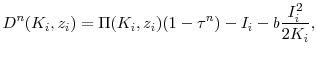
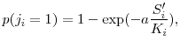
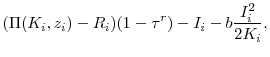
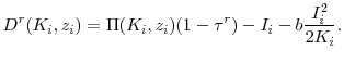
Firms in the R&D sector are similar to those in the non-R&D sector, except for their R&D activity. These firms also invest in a stock of R&D. The R&D stock of the firm does not directly impact the production function as in Griliches (1979) and others. Instead, the R&D stock stochastically affects the transition of profitability across periods. The model views R&D stocks as measuring the potential for future innovations rather than a measure of the stock of ideas applicable for production. When a firm's R&D activity is successful, the firm realizes a profitability jump in the next period.⁵ If the R&D effort was not successful, the firm will not realize a jump in profitability. These innovations reflect discoveries by firms that lead to an increased profitability of the firm's capital stock.⁶ A fraction of the R&D stock becomes obsolete each period reflecting the conclusion or abandonment of R&D projects. The model attempts to capture the inherently uncertain nature of the innovation process through this mechanism as a firm would realize a negative return from its R&D investment in a year in which it failed to innovate.

Denote the accumulated R&D stock of the firm at the end of each period by $S_i^{\prime }$ . Let equal the investment in R&D activity. The law of motion for R&D stocks is given by

$\displaystyle S_i^{\prime } = S_i (1-\gamma) + R_i,$

(A.6)

where $\gamma$ denotes the rate at which R&D stocks become obsolete. Let

denote a binary variable that equals 1 if the firm successfully innovates, and 0 otherwise. The probability of a successful innovation is given by a Bernoulli distribution with success probability

$\displaystyle p(j_i = 1) = 1 - \exp(-a\frac{S_i^{\prime }}{K_i}),$

(A.7)

where

is a parameter that influences the success rate of innovations. Higher R&D stocks lead to a greater probability of a successful innovation. This particular parametrization implies that success probabilities are concave in $S_i^{\prime }$ . The success probability decreases as the current capital stock increases. The scaling by capital stock can be thought of as capturing an increase in R&D project size with firm size. As such, larger firms require a greater level of R&D investment to generate the same probability of success as a small firm. The scaling ensures that large firms do not benefit disproportionately from R&D activity.⁷ In the event of success, log profitability jumps by a constant $\lambda$ .⁸ This measures the improvement in the firm's profitability from a successful innovation. The transition equation for profitability of firms in the R&D sector is as follows:

$\displaystyle \log(z_i^{\prime })$	$\displaystyle =$	$\displaystyle \mu + \rho \log(z_i) + \lambda j_i + \epsilon_i$	(A.8)
$\displaystyle j_i$	$\displaystyle \propto$	$\displaystyle \textsf{B}(p(\frac{S_i^{\prime }}{K_i}))$	(A.9)
$\displaystyle \epsilon_i$	$\displaystyle \propto$	$\displaystyle \textsf{N}(0, \sigma^2), \notag$	(A.10)

The distribution for

is independent of the distribution for $\epsilon_i$ . In this setup, the transition equation for profitability becomes an AR(1) process with jumps, where the jump intensity varies endogenously with R&D stocks.

The model is agnostic on the source of the jump in profits from a successful innovation. This may arise from either improvements in the current products of the firm, the introduction of entirely new products, or cost reductions. More formally, a successful innovation may result in an increase in the productivity parameter or the demand shifter . The model does not take a stand on whether patent protection is necessary for generating an increase in profitability (see Boldrin and Levine (2008)). While the inability to link R&D investment directly to total factor productivity may be a drawback, the above approach has the benefit of allowing R&D to have a broader impact. Correspondingly, the endogenous growth literature highlights both quality improvements and new product introductions as the outcome of innovations.

The timing of the firm's decisions warrant clarification. R&D sector firms enter each period with an R&D stock, a capital stock, and a profitability level. The firms invest in R&D and capital during the period. At the end of the period, each firm discovers whether it successfully innovated or not. If a firm succeeds, its next period profitability will be higher than if it did not. The accumulated R&D stock carries over to the next period and a fraction of it becomes obsolete after the realization of the profitability level $z^{\prime }$ . Note that this timing sequence differs from the law of motion for capital: the current period R&D investment adds to the R&D stock which impacts the realization of the next profitability level. This timing structure was chosen as it yields a value function that is separable in the R&D stock. It also captures the idea that R&D investment in the current period impacts the firm's profitability in the next period.

The dividends paid by the firm in each period is given by

$\displaystyle (\Pi(K_i, z_i) - R_i)(1-\tau^r) - I_i - b\frac{I_i^2}{2K_i},$

where $\tau^r$ denotes the linear tax rate paid by firms in the R&D sector. As in the tax code, R&D investment is treated as a tax deductible expense. Note that $\tau^r$ and $\tau^n$ may be different; these parameters will be calibrated using data on aggregate taxes and profits for each sector. The model thus incorporates differences in taxes payable by firms in the R&D sector and non-R&D sector in a parsimonious manner. These tax differences arise due to significantly higher leverage in the non-R&D sector as well as the research and experimentation tax credit. This tax credit is computed using a complex formula based on growth rates in R&D expenditures.

Denote the value of the firm after the realization of but prior to the obsolescence of the R&D stock as .⁹ For notational convenience, define

$\displaystyle D^r(K_i, z_i) = \Pi(K_i, z_i)(1-\tau^r) - I_i - b\frac{I_i^2}{2K_i}.$

(A.11)

The value of the firm can be expressed as a solution to the following Bellman equation:

$\displaystyle V^r(K_i, S_i, z_i)$	$\displaystyle =$	$\displaystyle \max_{I_i, K_i^{\prime }, R_i, S_i^{\prime }} D^r(K_i, z_i) - R_i(1-\tau^r) + \beta E_z[V^r(K_i^{\prime }, S_i^{\prime }, z_i^{\prime })],$	(A.12)
$\displaystyle K_i^{\prime }$	$\displaystyle =$	$\displaystyle K_i(1-\delta) + I_i, \notag$	(A.13)
$\displaystyle S_i^{\prime }$	$\displaystyle =$	$\displaystyle S_i (1-\gamma) + R_i, \notag$	(A.14)
$\displaystyle S_i^{\prime }$	$\displaystyle \ge$	$\displaystyle 0 \notag.$	(A.15)

The lack of a non-negativity constraint on R&D investment implies that firms can sell their R&D if necessary. While firms do so infrequently in the simulation, this assumption is necessary for the subsequent characterization of the R&D policy function. The reversibility assumption is also supported by anecdotal evidence of firms selling partially developed products to other firms, particularly in the pharmaceutical sector. The expectation in the Bellman equation is taken over the joint distribution for $j_i, \epsilon_i$ . The results in (Bertsekas, 2000, Chapter 7) yield the existence and uniqueness of the solution to the above problem. Substituting the expression for

into the maximization problem yields

$\displaystyle V^r(K_i, S_i, z_i)$	$\displaystyle =$	$\displaystyle \max_{I_i, K_i^{\prime }, S_i^{\prime }} D^r(K_i, z_i) + S_i (1-\gamma)(1-\tau^r) - S_i^{\prime }(1-\tau^r) + \beta E_z[V^r(K_i^{\prime }, S_i^{\prime }, z_i^{\prime })],$
$\displaystyle K_i^{\prime }$	$\displaystyle =$	$\displaystyle K_i(1-\delta) + I_i, \notag$
$\displaystyle S_i^{\prime }$	$\displaystyle \ge$	$\displaystyle 0 \notag.$

Observe that

does not impact the optimization problem for either $K_i^{\prime }$ or $S_i^{\prime }$ . This motivates the conjecture that the value of the firm can be simplified as follows:

$\displaystyle V^r(K_i, S_i, z_i) = G(K_i, z_i) + S_i(1-\gamma)(1-\tau^r).$

(A.16)

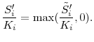
The value of the R&D stock equals $S_i(1-\gamma)(1-\tau^r)$ due to the model's timing convention. The value function is defined after the realization of

, but before the anticipated obsolescence of the R&D stock at the beginning of the period. Thus, the effective value of

equals its value after obsolescence, which is reduced by the tax deductability of R&D expenditures. Substituting the above expression into the Bellman equation, one obtains:

$\displaystyle G(K_i, z_i)$	$\displaystyle =$	$\displaystyle \max_{I_i, K_i^{\prime }, S_i^{\prime }} D^r(K_i, z_i) - S_i^{\prime }(1-\tau^r) + \beta S_i^{\prime }(1-\gamma)(1-\tau^r) + \beta E_z[G(K_i^{\prime }, z_i^{\prime })] ,$	(A.17)
$\displaystyle K_i^{\prime }$	$\displaystyle =$	$\displaystyle K_i(1-\delta) + I_i, \notag$	(A.18)
$\displaystyle S_i^{\prime }$	$\displaystyle \ge$	$\displaystyle 0 \notag.$	(A.19)

This establishes our conjecture and demonstrates that the value function is separable in the R&D stock. Note that this is not a general result, and it arose from the particular assumptions made about the timing and structure of the optimization problem. The separability ensures that the return to R&D investment is negative in periods where the firm does not innovate.

C R&D policy

The above analysis simplifies the solution of the optimal R&D policy of the firms. The optimal choice of $S_i^{\prime }$ impacts the current period dividend payment, the level of R&D stock carried over to the next period, as well as the transition equation for profitability . The first two pieces are linear in $S_i^{\prime }$ . Let $\tilde{S}_i^{\prime }$ be the optimal policy in the interior region, where the $S_i^{\prime } \ge 0$ constraint does not bind. The following proposition characterizes the optimal R&D stock in this region:

Proposition 1 The optimal R&D stock of the firm when $S_i^{\prime } > 0$ is given by

$\displaystyle \frac{\tilde{S}_i^{\prime }}{K_i} = \frac{1}{a} \left[\log(a) - \log\left((1-\tau^r)(1-\beta(1-\gamma))\right) + \log\left(\frac{\beta( E_z[G(K_i^{\prime }, z_i^{\prime })\vert j_i=1] - E_z[G(K_i^{\prime }, z_i^{\prime })\vert j_i=0])}{K_i}\right) \right].$

Proof. Appendix A. $\qedsymbol$

Therefore, the optimal policy function for R&D stocks is given by

$\displaystyle \frac{{S}_i^{\prime }}{K_i} = \max(\frac{\tilde{S}_i^{\prime }}{K_i}, 0).$

Optimal R&D investment increases with the expected jump in the value of the firm per unit of capital from a successful innovation. Decreasing returns to scale imply that $\frac{G(K_i, z_i)}{K_i}$ is decreasing in

. Therefore, the level of the optimal R&D stock per unit of capital decreases as firm size increases. This matches the negative relationship between firm size and R&D investment observed in the Compustat data set. The optimal R&D stock increases as the discount rate decreases.

The separability of the value function into its R&D stock and the above characterization of the R&D policy both simplify and improve the accuracy of the numerical solution of the value function in the subsequent estimation. The next section examines the return to R&D in this setting.

D Return to R&D

A key objective of estimating the above structural model is to identify the private return to R&D, defined as the marginal impact of R&D investment on next period after-tax profits. This definition closely mirrors that employed in the production function literature, where the return equals the marginal impact of R&D investment on next period value added. From an accounting perspective, the profits measure employed in the study equals the value added measure minus selling and administrative expenses. The impact of R&D on profits would be a more relevant variable for a firm's optimization decision than the impact of R&D on value added. Some algebra, detailed in Appendix B, yields the following expression for the expected return to R&D investment.

$\displaystyle \frac{\partial}{\partial{S_i{^\prime }}} E_z\left[ \Pi(K_i^{\prime }, z_i^{\prime })\right] = \left(\frac{(K_i^{\prime })^{\theta} z_i^{\rho} \exp\left(\mu + \sigma^2/2 \right) [\exp(\lambda) - 1]}{E_z[G(K_i^{\prime }, z_i^{\prime })\vert j_i=1] - E_z[G(K_i^{\prime }, z_i^{\prime })\vert j_i=0]}\right) \frac{\left(1 - \beta(1 - \gamma)\right)}{\beta}.$

(A.20)

The above expression lends itself to a natural interpretation in the context of the model. The first term equals the expected increase in next period profits from an innovation divided by the expected increase in firm value from an innovation. The $1 - \beta(1 - \gamma)$ term equals the residual value of R&D investment in the next period after obsolescence. Note that as the model incorporates the tax deductability of R&D investment, the comparable return definition would be the marginal impact on after-tax profits.

The intuition for the above formula arises from the fact that R&D policies are derived from optimality conditions. This implies that the discounted total marginal expected return to R&D investment equals its marginal cost, 1. Current period R&D investment affects the firm in the next period by increasing profits if the firm innovated and by increasing the residual R&D stock. An innovation also increases firm value, as expected profitability in subsequent periods increases, and as the firm optimally readjusts its capital stock in response to the innovation. The estimated return focuses only on the component of the total return measured in next period profits. Parameter changes that shift the total return from next period profits to an increase in firm value or that increase the residual value of R&D result in a lower estimated return. The maximum return of $\frac{1}{\beta}$ is obtained when $\rho = 0$ and $\gamma = 1$ . The estimated return increases with the obsolescence rate $\gamma$ . Note that changes in the parameter that influences the success probability, , impact the return indirectly through the $E_{z}[G(K_{i}^{\prime }, z_i^{\prime })\vert j_{i}]$ terms.

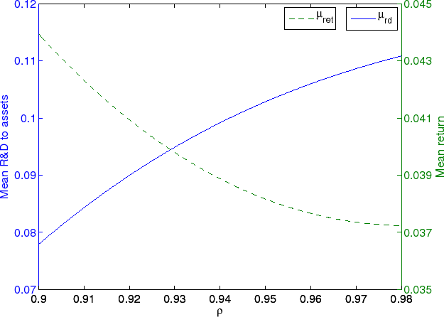
The return to R&D does not directly affect the optimal R&D policy in this setting, as they are both jointly determined. Figure 1 demonstrates the non-monotone relationship between optimal R&D investment and the return in the model. The figure plots the mean level of R&D investment on the left y-axis and the mean return to R&D on the right y-axis as the autocorrelation parameter, $\rho$ , increases from 0.90 to 0.98. The other parameters are fixed at the estimates obtained in Section 4.1. An increase in $\rho$ increases the benefit of an innovation and leads to an increase in the expected firm value from an innovation. This results in higher R&D investment. However, an increase in $\rho$ has no impact on the expected increase in next period profits from an innovation, leading to a decrease in the ratio of the expected increase in profits to firm value. This results in a reduction of the return as defined above.

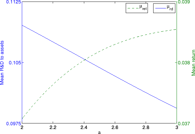
The non-monotone relationship between R&D investment and the return to R&D extends to changes in the parameter driving the success rate, . Figure 2 plots the mean level of R&D investment on the left y-axis and the mean return to R&D on the right y-axis as increases from 2 to 3. The other parameters are fixed at the estimates obtained in Section 4.1. For these parameters, an increase in leads to a decrease in optimal R&D as it lowers the probability of a successful innovation. This also lowers the growth options associated with R&D investment, thereby reducing the increase in firm value from an innovation while having no impact on the expected increase in profits from an innovation. Thus, an increase in leads to an increased return to R&D.

The above figures demonstrate that a high return to R&D does not imply a high level of R&D investment in this setting, or vice versa. Therefore, the return to R&D does not provide an appropriate statistic for forming R&D policies in the context of the model. The intuition for this result is that the R&D policy is determined by the expected total return to R&D, while the return focuses only on the expected impact on next period profits, which is only one component of the total return.

E Statistics of economic interest

The above analysis focuses on the return to R&D. The model also enables the computation of other statistics that may either be of independent interest or be useful in understanding R&D decisions.

The optimal R&D policy increases with the expected jump in firm value from an innovation. The percentage jump in firm value equals

$\displaystyle \frac{E_z[V^r(K_i^{\prime }, S_i^{\prime }, z_i^{\prime })\vert j_i=1] - E_z[V^r(K_i^{\prime }, S_i^{\prime }, z_i^{\prime })\vert j_i=0]}{E_z[V^r(K_i^{\prime }, S_i^{\prime }, z_i^{\prime })]}.$

While it is difficult to construct an empirical counterpart to the above measure, it is helpful for understanding R&D decisions.

The $\lambda$ parameter estimates the impact of an innovation on next period profits. The total impact of an innovation also depends on the speed at which the increase in profitability mean reverts. The present value equivalent permanent increase in profitability from an innovation provides an alternate method of evaluating the impact of an innovation on profits. This is given by:

$\displaystyle \frac{1-\beta}{1-\beta\rho}(\exp(\lambda)-1).$

The above statistic ignores changes in the optimal capital stock following an innovation. On the other hand, it provides a more direct comparison with quality ladder models of growth.

The model also provides an estimate of the value of the aggregate capital stock, which includes both physical capital and R&D stocks. The expected value of the R&D stock of each firm is given by

$\displaystyle E_z[V^r(K^{\prime }_i, S^{\prime }_i, z^{\prime }_i)] - E_z[V^n(K^{\prime }_i, z^{\prime }_i)],$

which equals the difference in market value between a firm in the R&D sector with one in the non-R&D sector with the same capital stock and profitability levels. This includes the book value of the R&D stock plus the growth opportunities associated with it. The ratio of the aggregate R&D stock to the value of all capital within the R&D sector can be obtained as

$\displaystyle \frac{\sum_i \left(E_z[V^r(K^{\prime }_i, S^{\prime }_i, z^{\prime }_i)] - E_z[V^n(K^{\prime }_i, z^{\prime }_i)\vert z_i]\right)}{\sum_i E_z[V^r(K^{\prime }_i, S^{\prime }_i, z^{\prime }_i)\vert z_i]}.$

The value of the aggregate R&D stock as a fraction of all capital equals the above expression times the market value of the R&D sector as a fraction of the market value of all firms, which is obtained from the data and equals 0.723.

3 Estimation

The study estimates the above models using indirect inference, a variant of simulated methods of moments estimation (see Gourieroux, Monfort, and Renault (1993) for details). This method involves comparing a selected set of data moments with the same moments from artificial data obtained by simulating the model for a given set of parameters. The parameter estimates are obtained as the solution to the minimization of a quadratic form of the difference between the data and simulated moments. Appendices C and D discuss the estimation in more detail.

A Data

The data for the estimation is obtained from the Compustat Annual data set. The data set includes information on profits, capital expenditures, and balance sheet items for listed US corporations. The market value of equity is obtained from the linked CRSP data set. The sample period extends from 1987 to 2006, and was chosen to provide a stable tax environment for research and development expenditures. The sample excludes financial firms and regulated utilities.

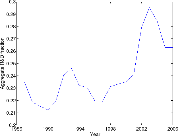
Figure 3 plots R&D investment as a fraction of the sum of R&D and physical investment over time. The figure demonstrates the substantial level of investment in R&D conducted by US corporations. This provides suggestive evidence that the return to R&D is lower than widely believed as it would be difficult to reconcile the high level of R&D investment with the substantial private returns reported in the literature (Griliches (1994)) under standard concavity assumptions. The high level of R&D investment also suggests that calibrations and estimations of RBC models may be misspecified when they do not take into account R&D investment.

The data on research and development expenditures (Compustat Annual data item 46) is available for more than half the observations. This series measures company funded R&D and excludes those funded by the government. As such, the results in this study measure the return to private R&D. About 11% of the sample reports a zero value for R&D spending. One key choice in this paper is to treat firm-year observations with missing or zero values for R&D expenditures as firms in the non-R&D sector. The results would be biased if some of these firms engage in substantial R&D activity. Accounting rules provide some comfort in this regard, as they clearly specify the classification and reporting of R&D expenditures. Furthermore, most firms that report positive values for R&D expenditures do so for all years, while many firms do not engage in any R&D expenditures at all. The fraction of such observations in the data equals 87.75%.¹⁰ This indicates that the data can be separated into two sectors: an R&D sector with positive R&D expenditures and a non-R&D sector with zero spending on R&D. The method of moments estimation matches first and second moments on data from the two sectors.

The production function regressions require the construction of the R&D stock for each firm. The R&D stock for an assumed obsolescence rate was constructed using a perpetual inventory method, with historical R&D expenditures from 1975 onwards. The initial R&D stock was obtained assuming a real growth rate of 5%. The initial assumptions have little impact, as the regressions use observations from 1987 onwards, matching the sample selection for the structural estimation. The log value added measure is obtained as net sales (data item 12) minus cost of goods sold (data item 41). All variables except employment are adjusted for inflation using the GDP deflator for non-residential investment.

Table 1 provides summary statistics for firms in the R&D and non-R&D sectors. Total assets equals the book value of assets (data item 6). Profits equals operating income before depreciation (data item 13) scaled by book assets. Investment is defined as capital expenditure on plant, property, and equipment (data item 30) minus retirements of plant, property, and equipment (data item 184). Tobin's Q is computed as the market value of assets scaled by the book value of assets.¹¹ An alternative definition would be to define Q as the market value of capital scaled by the replacement value of capital. While this definition may be preferred where measurement error is a concern (Erickson and Whited (2000)), it also leads to large outliers, particularly in the R&D sector, that may bias the comparison between the two sectors. The variables are Winsorized at the 99% level to eliminate outliers. The data used to compute the matched moments are adjusted for firm and year fixed effects within the R&D and non-R&D sectors, respectively.

The moments demonstrate a sharp contrast between these two sectors, indicating fundamental differences between firms that engage in R&D activity and those that do not. These differences are statistically significant at the 1% level. Firms in the R&D sector have an average Tobin's Q value almost 50% greater than firms in the non-R&D sector (Chan, Lakonishok, and Sougiannis (2001) find that the market value of the firm reflect R&D activity). On the other hand, these firms exhibit much lower average earnings after accounting for their R&D expenditures. The level of R&D spending is quite substantial when compared to total assets and larger than the rate of investment. However, aggregate expenditures on R&D are lower than total capital expenditures within the R&D sector, as small firms do a disproportionately larger level of R&D spending. This is consistent with the R&D policy function given in Proposition 1 as smaller firm capture a greater increase in firm value per unit of capital from an innovation.

B Identification

The results obtained from indirect inference methods are sensitive to the choice of which specifics moments are to be matched. In particular, it is important to select moments that are informative about the parameters of interest. Intuitively, if a given simulated moment varies strongly with a parameter, matching this moment to the data will be informative about the underlying parameter.

The moments I match include the first moment of profits for the R&D and non-R&D sectors. This will be informative about the parameters of the profitability process, as well as the parameters influencing the success rate and impact of R&D spending. The second moments of profits for both sectors help identify $\sigma$ . The first and second moments of R&D spending provide information on the R&D parameters $\lambda, a,$ and $\gamma$ . The first moments of Tobin's Q for each sector help inform the returns to scale parameter $\theta$ and the R&D parameters. The second moments of Q for both sectors also help identify $\theta$ and the volatility of profits. The autocorrelation coefficient for profits and R&D spending helps inform the $\rho$ parameter. Finally, the second moment of investment identifies the level of adjustment cost parameter . It should be noted that each moment provides information on almost all of the parameters.

All moments do not have the same weight in the estimation. The optimal weighting matrix is obtained as the inverse of the covariance matrix of the chosen moments. Intuitively, the GMM estimation works harder to match the more precisely estimated moments. Standardizing the chosen moments by their standard errors reveals that the estimation places little weight on matching the autocorrelation for R&D, and emphasizes the first moment of R&D, the first moment of Q for both sectors, and the first moment of operating income for the non-R&D sector.

Some of the auxiliary parameters in the model are calibrated to simplify the estimation of the parameters of interest. The calibrated parameters are the discount factor $\beta$ , the per period fixed cost of operations and the depreciation rate $\delta$ . The calibrated value of $\beta = 1/1.065$ follows Gomes (2001), Hennessy and Whited (2005), and Bloom (2008) and reflects an equity premium of 6%. The fixed cost of operation is set at 15% of the profits prior to R&D expenditure for the median firm in each sector.¹² The depreciation rate $\delta = 0.079$ , a value which equals the mean investment rate for all firms from the data. Setting the depreciation rate equal to the investment rate in the data ensures that the steady state investment rate in the simulated data, which equals the depreciation rate, matches the actual data. One could easily match the mean investment rates for the two sectors separately by specifying different depreciation rates. The fraction of firms in the R&D sector equals 0.48, the fraction of observations with positive R&D values in the data set. The $\mu$ parameter is not identified with the chosen moments as it functions as a scaling parameter. As such, fix $\mu =-0.3$ for both sectors. The chosen moments do not include the relative firm size between R&D and non-R&D firms. This could be matched by allowing $\mu$ to vary across the two sectors.

C Estimating the return using production functions

This section details the observation that the production function approach pioneered by Griliches (1979) suffers from an indeterminacy flaw when applied to estimating the return to R&D. This approach specifies value-added by the firm as a multiplicative function of factor inputs, including the R&D stock:

$\displaystyle Y_{i,t} = a_t K_{i,t}^{\alpha}L_{i,t}^{\beta}S_{i,t}^{\nu}.$

(A.21)

A linear regression of log value-added on log inputs yields the elasticity of value-added with respect to the R&D stock $\nu$ . The construction of the R&D stock $S_{i,t}$ follows a perpetual inventory method using data on R&D expenditures applied to equation (4). The obsolescence rate of R&D investment necessary for the construction of the R&D stock is typically assumed to be 15%, following Griliches and Mairesse (1984), or sometimes assumed to be 0. One common finding in this literature is that the estimated elasticity $\nu$ does not vary with the assumed obsolescence rate $\gamma$ .

The return to R&D in this framework equals the marginal product of R&D on value-added and is given by:

$\displaystyle \frac{\partial{Y_{i,t}}}{\partial{S_{i,t}}} = \nu \frac{Y_{i,t}}{S_{i,t}}.$

The calculated R&D stocks vary with the assumed obsolescence rate $\gamma$ . This can be most easily seen by considering a firm that invests a fixed amount

in R&D. The R&D stock of this firm is given by $S = \frac{R}{\gamma}$ . However, while the calculated R&D stocks vary with $\gamma$ , the $\nu$ estimates does not (Hall and Mairesse (1995)). This implies that the estimated rates of return obtained using this framework are sensitive to the assumed obsolescence rate $\gamma$ . The intuition for this result is that higher obsolescence rates lead to a lower R&D stock, resulting in a higher marginal impact of R&D on value added, as the elasticity parameter remains mostly unchanged.

Table 2 presents the results of the above regression for different assumptions on $\gamma$ using the Compustat data set. Note that even though the notation is identical, $\gamma$ may not be comparable across the two approaches as the R&D stock concept in the production function regression differs from the R&D stock concept in the structural model. The sample ranges from 1987 to 2006, and all variables except employment are adjusted for inflation using the GDP deflator for non-residential investment. The pooled regression includes year and industry dummies, and the standard errors are robust to clustering at the firm level. The assumed obsolescence rates range from 0 to 0.25.

The regressions reveal that the estimated elasticity of value-added with respect to R&D varies little with the obsolescence rate $\gamma$ , as commonly found in the literature. The point estimate implies an economically and statistically significant contribution of R&D to value-added by firms. The adjusted R-square values indicate that the model fit does not vary much with $\gamma$ .

The table reports the sample median steady state return for a hypothetical firm with a constant R&D policy and the sample median return using the computed R&D stocks. Both return estimates vary sharply with the obsolescence rate $\gamma$ . Using the standard assumption of $\gamma = 0.15$ leads to an estimated median return of 45.2%, similar to the high rates of return reported in the literature (see Griliches (1986) and Hall and Mairesse (1995)). However, changing the assumed value of $\gamma$ to 0 yields a much lower return (12.6%), and assuming $\gamma = 0.25$ yields an even higher return. The steady state returns with a fixed R&D policy exhibit similar variation. Thus, the return estimates obtained from production function regressions vary sharply with the assumed obsolescence rates, a difficulty compounded by the lack of evidence on the appropriate value for $\gamma$ .

4 Results from structural estimation

A Baseline model

The estimation begins with the baseline model, which identifies the impact of R&D on profits, the success rate from R&D, and the rate of depreciation for R&D stocks. Table 3 presents the results of estimating the model by indirect inference. Panel A reports the matched moments for the data and simulations, respectively. Panel B reports the estimated parameter values. Panel C reports some statistics of economic interest from the simulated data set.

The low value for the J-statistic demonstrates that the model matches the chosen moments well. Examination of the matched moments indicates that the model succeeds in matching the first and second moments of R&D to assets. The model also matches the first moment of Tobin's Q for both sectors, and matches the second moment of Tobin's Q for the non-R&D sector. While the measure of Tobin's Q in the simulated data incorporates the R&D stock it also reflects differences in growth options due to potential innovations. The model fares less well at matching the first and second moments of income for both sectors. The estimation yields a $\rho$ value that is much higher than regression estimates, thereby resulting in higher autocorrelations for both profits and R&D expenditures.

The model has trouble generating the high level of Tobin's Q given the observed levels of profits. A related difficulty arises from matching the variation in Tobin's Q given the variation in profits. A high autocorrelation value helps with both of these challenges. For a given distribution of profits, an increase in persistence will increase Tobin's Q for high profitability firms and lower it for low profitability firms. This impact will be greater for high Q firms, resulting in higher first and second moments for Tobin's Q. A high autocorrelation value also increases R&D investment by extending the benefit of an innovation further into the future.

The results indicate that firms in the R&D sector generate an economically and statistically significant increase in profitability from a successful innovation. The point estimate for $\lambda$ of 0.123 implies that a successful innovation increases the profitability of the firm by 13.1%. Ignoring any changes in the capital stock, this is equivalent in present value terms to a 9.0% permanent increase in profitability. In the steady state, 50.7% of firms in the R&D sector innovate each period. However, there is sharp cross-sectional variation in the probability of innovation, reflecting the sensitivity of the R&D policy function on the current profitability and size of the firm.

An application of equation (12) yields the distribution of the expected return to R&D in the simulations. The simulations yield a mean return of only 3.7%, with a 95th percentile value of 8.2% (multiplying by $1/(1-\tau^r) = 1.24$ yields the pre-tax return). These values are substantially lower than commonly believed. The residual value of R&D investment at the end of the next period equals $0.714 (= \beta*(1-\gamma))$ , implying a maximum expected return of 30.5%. The return is driven lower by the high $\rho$ parameter, which shifts the benefits of an innovation further into the future. This decreases the ratio of expected increase in next period profits from an innovation to the expected increase in firm value. While the return is much lower than those reported in the literature, that does not deter firms from maintaining a high level of R&D investment.

The estimated obsolescence rate of $\gamma = 0.240$ is not directly comparable to the values employed in the production function approach. The R&D stock in the model pertains only to the R&D investments applicable to generating the next innovation. Prior innovations from R&D would be reflected in a higher level of profitability . In contrast, the R&D stock in the production function approach reflects all the accumulated knowledge application for production. The estimated high obsolescence rate indicates that a substantial proportion of a firm's R&D expenditures ceases to have any value if the firm fails to innovate. Hall (2007) obtains obtains similarly high estimates of $\gamma$ using a valuation based approach, thus providing support for this study's view of R&D stocks as measuring the stock of experiments towards the next innovation. It is less plausible to view the stock of ideas applicable for production becoming obsolete at these rates. The $\gamma$ estimate implies a half-life of R&D expenditures of 2.53 years, indicating a moderate lifespan for R&D projects. The point estimate for the adjustment cost parameter matches those found by Whited (1992), Cooper and Haltiwanger (2006), and Eberly, Rebelo, and Vincent (2008).

The steady state mean expected increase in firm value equals $21.3\%$ , with a high degree of cross-sectional variation. A high impact of innovation on firm value induces firms to incur the high level of R&D expenditures observed in the data and the simulations despite the low return estimates. While the appropriate sample counterpart is unclear, the estimate is consistent with anecdotal evidence of sudden jumps in firm value upon the release of news about potential innovations.

The estimation yields a value of the aggregate R&D stock equal to 17.9% of the value of all capital.¹³ In comparison, the aggregate value of R&D investment to all investment in the sample period equals 24.6%. This indicates that a substantial portion of the aggregate capital stock consists of R&D stocks. As R&D stocks comprise a large fraction of all intangible capital, these findings support the argument of Hall (2001) that intangible capital accumulation forms an important component of US investment.

B Estimates with a lower discount rate

The estimates of the baseline model indicate that the model has difficulty reconciling the profit and valuation levels. This has the effect of yielding a very high autocorrelation parameter, as the model strives to reconcile a low level of profits with the observed valuations. One solution to this difficulty is to assume a lower discount rate. The value of $\beta = 1/1.065$ used in the baseline estimation is calibrated assuming a 6% equity premium. Recent evidence indicates that the equity premium may have been sharply lower for this sample period, motivating a higher value for $\beta$ . This section reports the results using a discount rate of $\beta = 1/1.045$ to estimate the model.¹⁴

Table 4 presents the results using the lower discount rate. Panel A reports the matched moments for the data and simulations, respectively. Panel B reports the estimated parameter values. Panel C reports some statistics of economic interest from the simulated data set.

The value of the J-statistic is lower than that for the baseline model. As suggested above, this model has better success reconciling the moments on profits with the valuation moments. The lower discount rate also leads to a lower autocorrelation parameter. The estimates continue to have difficulty with the second moment of Tobin's Q, as the model does not generate as many observations with high Tobin's Q as found in the data. Overall, the lower discount rate improves the performance of the model.

The point estimate for $\lambda$ implies a 18.9% increase in profitability from a successful innovation. This is larger than the corresponding value obtained in the baseline estimation because the lower value of $\rho$ requires an innovation to have a greater initial impact on profits, as the benefit dissipates faster. In present value terms, the estimate corresponds to a 4.63% permanent increase in profitability, lower than the comparable estimate for the baseline model. The smaller permanent increase in profits generates a similar level of R&D expenditures, as the firms discount future dividends less than before. The steady state rate of innovation is lower, with a mean probability of success of 0.450.¹⁵ This is partly due to the higher obsolescence rate $\gamma$ , which implies a lower steady state R&D stock than in the baseline model.

The steady state mean return to R&D expenditures equals 5.5%, higher than the estimated value from the baseline model. Nonetheless, this estimate is much lower than the values reported in the literature. Intuitively, the lower estimate for $\rho$ implies that more of the benefit of an innovation is realized in the next period, thereby increasing the ratio of expected increase in profits from an innovation to the expected increase in firm value. The higher estimate of $\gamma$ decreases the residual value of R&D expenditures, also resulting in a higher return. However, the higher return does not translate to a higher level of R&D expenditures.

The difference in expected firm value from innovating versus not-innovating has a direct impact on R&D policy in the model. The mean expected increase in firm value of $14.1\%$ is lower than the corresponding value in the baseline model. There is also much less cross-sectional variation in the increase in firm value. The higher impact of a successful innovation on profits does not translate to firm values, as the benefit dissipates faster.

C Estimates using only R&D sector data

The results presented in the baseline model assume that the non-R&D related parameters are identical across both sectors and use non-R&D sector data to help estimate these parameters. However, these parameters may vary across the two sectors. This section presents the results of estimating the model using data only on R&D sector firms. This leads to a decrease in the number of matched moments and provides a robustness check to differences in model parameters across the two sectors.

Table 5 presents the results of estimating the model using indirect inference with data on R&D sector firms only. Panel A reports the matched moments for the data and simulations, respectively. Panel B reports the estimated parameter values. Panel C reports some statistics of economic interest from the simulated data set. The calibrated value of $\delta = 6.3\%$ , the mean capital investment rate for R&D sector firms. The discount rate $\beta = 1/1.065$ , as in the baseline model.

The matched moments exhibit a similar pattern to that observed in Table 3. The model matches the first and second moments of R&D and has difficulty reconciling the level of profitability with the level of Tobin's Q. The model also implies a higher autocorrelation level for profits and R&D than found in the data. The -statistic increases and its -value decreases, as the number of data points and the degrees of freedom decrease. However, the data does not reject the model.

The point estimates imply a higher impact of an innovation on profits and a higher obsolescence rate for R&D expenditures. The lower point estimate for $\theta$ suggests that mark-ups may be slightly higher in the R&D sector. Somewhat surprisingly, the measures of economic interest are quite similar to those obtained using data on both sectors. The return to R&D is, as before, much lower than that reported in the literature. The probability of an innovation exhibits sharp cross-sectional variation and is slightly lower than the baseline model estimate.

The above estimates indicate that firms capture an economically and statistically significant increase in profits from innovation. They also face significant uncertainty regarding the outcome of their R&D expenditures. This uncertainty does not, however, deter firms from undertaking the substantial level of R&D expenditures observed in the data.

5 Policy experiments

This section presents the results of counterfactual experiments on the following: a subsidy on R&D spending and an increase in the impact of a successful innovation on profits. The policy experiments reflect the model and are partial equilibrium in nature. They do not take into account possible responses by consumers or changes in government spending arising from these exogenous changes. As such, substantial care needs to be taken in using these experiments to argue for policy changes. The analysis provides a method to quantify the impact of changes in key parameters on the level of R&D spending, profits, firm value, and the rate of innovation within the context of the model.

A A subsidy to R&D spending

There exists an active policy debate about using the tax code to subsidize R&D investment. The research and experimentation tax credit uses a complex formula based on growth rates in these expenditures, which comprise only a subset of total R&D expenditures. The estimation presented in the previous section accounts for the tax credit through the calibration of the gross tax rate on operating income, $\tau^r$ . The tax credit amounted to about 2.5% of all spending on R&D by firms from 1990 to 2001 (Moris (2005)). Currently, the tax credit is not permanent and requires Congressional authorization every few years. This counterfactual experiment studies the impact of a further 5% R&D tax credit within the context of the model (see Bloom, Griffith, and van Reenen (2002) for a cross-country study on the impact of tax subsidies on innovation). Table 6 reports the moments of interest using the actual estimates and with a 5% subsidy on R&D expenditures. Panel A reports the values for the baseline model, Panel B reports the values with the lower discount rate parameter, and Panel C reports the results with the R&D sector only estimates. While the analysis does not impose any other taxes to offset the drop in tax revenue, it can provide a basis for a cost-benefit analysis of R&D tax credits.

The subsidy for R&D expenditures leads to higher spending and a greater level of innovation under all models. The tax subsidy increases the rate of innovation by 4.4, 3.6, and 4.4 percentage points for the models estimated in Sections 4.1, 4.2, and 4.3, respectively. This is driven by an approximately 1% increase in the rate of R&D expenditures in response to the additional tax credit. The findings imply a mean increase in R&D expenditures of 1.72 to 2.15 dollars for a dollar increase in the R&D tax credit. This is higher than the 1 to 1 impact of R&D tax credits on R&D expenditures estimated by Hall and van Reenen (2000). The similar impact of the tax subsidy for all models contrasts with the different rates of return. This provides further evidence that using the return to R&D for policy prescriptions leads to erroneous conclusions in this setting.

B An increase in the impact of a successful innovation

An increase in the impact of a successful innovation provides a method to incorporate changes in patent policy that favor innovators into the model. Eaton and Kortum (1999) directly estimate a model of international research and patenting and find a strong effect of strengthening patent rights on productivity growth. While such an analysis does not shed much light on the optimal level of patent protection, it can help quantify the impact of a change in patent policy on R&D expenditures and the rate of innovation. Gilbert and Shapiro (1990) argue for viewing patent policy in terms of the degree of profits accruing to the innovator. In the context of this study, increased patent protection can be viewed as an exogenous increase in $\lambda$ . Table 7 reports the moments of interest using the actual estimates and the new values obtained with a 5% increase in $\lambda$ . Panel A reports the values for the baseline model, Panel B reports the values with the lower discount rate parameter, and Panel C reports the results with the R&D sector only estimates.

The increase in the impact of a successful innovation on profits leads to higher investment in R&D for all models. The rate of innovation increases by 3.7, 3.2, and 3.6 percentage points, respectively. The increase in $\lambda$ has a similar impact on the rate of innovation as the R&D tax subsidy. However, this experiment has a larger impact on valuation compared to the tax subsidy. The tax subsidy benefits all R&D firms, while the increase in $\lambda$ benefits only firms that innovate. As firms with higher valuations invest more in R&D and are more likely to innovate, the change in $\lambda$ has a bigger impact on these firms, as reflected in the larger increase in the mean value of Tobin's Q.

6 Conclusion

An empirical analysis demonstrates that the high returns to R&D found in much of the literature are sensitive to assumptions of the obsolescence rate. This study estimates the return to R&D by simultaneously estimating all the key structural parameters of a dynamic model. The underlying model differs from that used in the production based approach as it incorporates uncertainty in the outcome of R&D projects, an arguably key economic feature of R&D investment. Further, the R&D stock in the model measures investment made towards generating the next innovation instead of the knowledge stock applicable for production. The identified variables of interest include the impact of an innovation on profits, the rate of innovation, the return to R&D, and the expected increase in firm value from an innovation.

The estimates reveal an economically and statistically significant impact of an innovation on profits. In present value terms, an innovation leads to an increase in profitability of 4.6-9.0%. This translates to an expected increase in firm value from innovating of 14.1-21.3%. The estimated rates of innovation suggest a significant probability of failure for R&D projects, highlighting the importance of uncertainty in estimating the return to R&D. The estimated returns to R&D are much lower than those found in the literature. However, this does not deter firms from maintaining a high level of R&D investment.

Counterfactual experiments examine the impact of a subsidy to R&D expenditures and an increase in profits from a successful innovation. A tax subsidy yields a clear increase in the rate of innovation even though the estimates imply a low return. These findings suggests that, as it focuses only on the short-term impact, the return to R&D would not be an appropriate tool for R&D policy analysis.

The analysis in this study employs a partial equilibrium approach that does not incorporate economic growth. Combining the findings of this study with endogenous growth models, such as that by Klette and Kortum (2004), may provide a rich framework for further research and policy analysis.

Appendix

A Proofs

Proposition 1 The optimal R&D stock of the firm when $S_i^{\prime } > 0$ is given by

Proof. The first order condition for the optimal R&D stock yields:

$\displaystyle -(1-\tau^r) + (1-\tau^r)\beta(1 - \gamma) + \beta \frac{\partial{E_z[G(K_i^{\prime }, z_i^{\prime })]}}{\partial{S_i^{\prime }}} = 0.$

(A.1)

The impact of R&D spending on the expected value of the firm in the next period can be clarified by an application of the law of iterated expectations,

$\displaystyle E_z[G(K_i^{\prime }, z_i^{\prime })] = E_z[G(K_i^{\prime }, z_i^{\prime })\vert j_i=1]p(j_i=1) + E_z[G(K_i^{\prime }, z_i^{\prime })\vert j_i=0]p(j_i=0).$

This result arises due to the independence between the draws of

and $\epsilon_i$ . Substituting the expression for

given in (5) one obtains:

$\displaystyle E_z[G(K_i^{\prime }, z_i^{\prime })] = E_z[G(K_i^{\prime }, z_i^{\prime })\vert j_i=1](1-\exp(-a\frac{S_i^{\prime }}{K_i})) + E_z[G(K_i^{\prime }, z_i^{\prime })\vert j_i=0]\exp(-a\frac{S_i^{\prime }}{K_i}).$

(A.2)

The derivative of the above expression with respect to $S_i^{\prime }$ yields:

$\displaystyle \frac{\partial{E_z[G(K_i^{\prime }, z_i^{\prime })]}}{\partial{S_i^{\prime }}} = \frac{a}{K_i}\exp(-a\frac{S_i^{\prime }}{K_i})\left(E_z[G(K_i^{\prime }, z_i^{\prime })\vert j_i=1] - E_z[G(K_i^{\prime }, z_i^{\prime })\vert j_i=0]\right).$

Substituting the above expression into the first order condition given in (A.1) yields the optimal policy function for the firm's R&D stock,

		$\displaystyle (1-\tau^r)(1 - \beta(1 - \gamma)) = \beta \frac{a}{K_i}\exp(-a\frac{\tilde{S}_i^{\prime }}{K_i})\left(E_z[G(K_i^{\prime }, z_i^{\prime })\vert j_i=1] - E_z[G(K_i^{\prime }, z_i^{\prime })\vert j_i=0]\right)$	(A.3)
		$\displaystyle \Rightarrow \frac{\tilde{S}_i^{\prime }}{K_i} = \frac{1}{a} \left[\log(a) - \log\left((1-\tau^r)(1-\beta(1-\gamma))\right) + \log\left(\frac{\beta( E_z[G(K_i^{\prime }, z_i^{\prime })\vert j_i=1] - E_z[G(K_i^{\prime }, z_i^{\prime })\vert j_i=0])}{K_i}\right) \right]. \notag$	(A.4)

Some algebra reveals that the second order condition with respect to $S_i^{\prime }$ is negative, ensuring that the F.O.C.s yield the optimal policy in the interior region. $\qedsymbol$

B Expected return to R&D

The after-tax expected return to R&D expenditures is given by:

$\displaystyle \frac{\partial}{\partial{S_i{^\prime }}} E_z\left[ \Pi(K_i^{\prime }, z_i^{\prime })(1-\tau^r)\right] = \frac{\partial}{\partial{S_i{^\prime }}} E_z\left[ z_i^{\prime }(K_i^{\prime })^{\theta}(1-\tau^r)\right].$

(B.1)

The conditional expectation of $z_i^{\prime }$ can be written as,

$\displaystyle E_z[z_i^{\prime }] = E_z[z_i^{\prime }\vert j_i=1] p(j_i=1) + E_z[z_i^{\prime }\vert j_i=0] p(j_i=0).$

(B.2)

Using the transition equation for $z_i^{\prime }$ in (6) and the log-normality assumption, the conditional expectations can be written as

$\displaystyle E_z\left[z_i^{\prime }\vert j_i=1\right]$	$\displaystyle =$	$\displaystyle \exp\left(\mu + \lambda + \rho\log(z_i) + \sigma^2/2\right)$
	$\displaystyle =$	$\displaystyle z_i^{\rho} \exp\left(\mu + \sigma^2/2 + \lambda \right).$
$\displaystyle E_z\left[z_i^{\prime }\vert j_i=0\right]$	$\displaystyle =$	$\displaystyle z_i^{\rho} \exp\left(\mu + \sigma^2/2 \right).$

The partial derivative of the probability of an innovation equals:

$\displaystyle \frac{\partial}{\partial{S_i{^\prime }}}p(j_i=1) = \frac{a}{K_i} \exp(-a\frac{S_i^{\prime }}{K_i}).$

(B.3)

The above expressions yield the following:

$\displaystyle \frac{\partial}{\partial{S_i{^\prime }}} E_z\left[\Pi(K_i^{\prime }, z_i^{\prime })\right]$	$\displaystyle =$	$\displaystyle (K_i^{\prime })^{\theta} \left[z_i^{\rho} \exp\left(\mu + \sigma^2/2 + \lambda \right) \frac{a}{K_i} \exp(-a\frac{S_i^{\prime }}{K_i}) - z_i^{\rho} \exp\left(\mu + \sigma^2/2 \right) \frac{a}{K_i} \exp(-a\frac{S_i^{\prime }}{K_i}) \right]$
	$\displaystyle =$	$\displaystyle (K_i^{\prime })^{\theta} \frac{a}{K_i} \exp(-a\frac{S_i^{\prime }}{K_i}) z_i^{\rho} \exp\left(\mu + \sigma^2/2 \right) [\exp(\lambda) - 1].$

Substituting the expression for $\frac{a}{K_i} \exp(-a\frac{S_i^{\prime }}{K_i})$ given in (A.3) and collecting terms yields the following expression for the return to R&D.:

C Simulated method of moments

The indirect inference method of Gourieroux, Monfort, and Renault (1993) obtains parameter estimates by matching a set of selected moments from the data to those obtained by simulation. Denote the structural parameters by $\Psi^{*}$ . The matched moments can be written as a solution to a minimization problem , where denotes the data and the moments to be matched. The data moments are then given by

$\displaystyle \hat{M} = \arg\min_M Q(Y_N, M),$

(C.1)

where

denotes a data matrix with

observations. The corresponding moments for the simulated data set with parameter vector $\Psi$ and $n = N \times S$ observations are given by

$\displaystyle \hat{m}(\Psi) = \arg\min_M Q(Y_m, M).$

(C.2)

The study picks

, which is within the recommended range.

The structural parameters are then obtained by minimizing a quadratic form of the distance between the data and simulated moments.

$\displaystyle \hat{\Psi} = \arg\min_\Psi \left[\hat{M} - \hat{m}(\Psi)\right]' \hat{W} \left[\hat{M} - \hat{m}(\Psi) \right],$

(C.3)

where $\hat{W}$ denotes a positive definite weighting matrix. The optimal weighting matrix is given by

$\displaystyle \hat{W} = \left[N \text{var}(\hat{M}) \right]^{-1}.$

(C.4)

The above covariance matrix is calculated with the actual data set using the influence function method of Erickson and Whited (2000). The estimator is asymptotically normal for fixed

with covariance matrix given by

$\displaystyle \sqrt{N}(\hat{\Psi} - \Psi^{*})$	$\displaystyle \sim$	$\displaystyle \textsf{N}(0, \Phi)$	(C.5)
$\displaystyle \Phi$	$\displaystyle =$	$\displaystyle (1 + \frac{1}{S}) \left[\frac{\partial^2{Q}}{\partial{\Psi}\partial{M}'} \left(\frac{\partial{Q}}{\partial{M}}\frac{\partial{Q}}{\partial{M}}'\right)^{-1} \frac{\partial^2{Q}}{\partial{M}\partial{\Psi}'}\right]^{-1}. \notag$	(C.6)

While $\frac{\partial{Q}}{\partial{M}}$ can be evaluated analytically, numerical methods are required to obtain $\frac{\partial^2{Q}}{\partial{\Psi}\partial{M}}$ . Both partial derivatives are obtained using simulated data evaluated at the data moments.

The indirect inference method also yields a GMM-style test of the over-identifying restrictions. The -statistic adjusted for the simulation size converges in distribution to a $\chi^2$ distribution, with degrees of freedom equal to the number of moments minus the number of parameters:

$\displaystyle J = \frac{NS}{1+S} \left[\hat{M} - \hat{m}(\Psi)\right]' \hat{W} \left[\hat{M} - \hat{m}(\Psi) \right].$

(C.7)

D Numerical Solution

The simulations require numerical solution of the value function for firms in the R&D and non-R&D sectors. The capital grid has 61 points and the profits grid has 10 points. The capital grid is centered around an approximation of the median size of the firm given the parameters. Simulations which result in steady state firm sizes near the boundaries of the grid are discarded in the estimation. The profit grid is formed using the quadrature method of Tauchen and Hussey (1991), with a mean value obtained by guessing the success rate. The endogenous jumps in from an innovation are handled by interpolating firm value over two more grids constructed using the transition equation for profitability conditional on whether the firm innovates. The expected value of the firm is obtained using the law of iterated expectations.

The simulated sample is generated using the value and policy functions for the R&D and non-R&D sectors. The law of motion for profitability is generated directly using the transition equations (6) and (2). The firm's decisions are obtained using linear interpolation of the policy functions. The simulations maintain the same fraction of firms in the R&D sector as in the data. The simulation is run for 100 years, with the initial 50 discarded as a burn-in sample. This yields the value of the quadratic form of the difference in the data moments and simulated moments. The program searches for the parameters that minimize this distance using the simulated annealing algorithm. Each estimation involved evaluating more than 100,000 candidate parameter sets.

Bibliography

ABEL, ANDREW, AND JANICE C. EBERLY

1994, A unified model of investment under uncertainty, American Economic Review 84, 1369-1384.

AGHION, PHILIPPE, NICK BLOOM, RICHARD BLUNDELL, RACHEL GRIFFITH, AND PETER HOWITT

2005, Competition and innovation: An inverted-U relationship, Quarterly Journal of Economics 120, 701-728.

AGHION, PHILIPPE, AND PETER HOWITT

1992, A model of growth through creative destruction, Econometrica 60, 323-351.

BARLEVY, GADI

2007, On the cyclicality of research and development, American Economic Review 97, 1131-1164.

BERTSEKAS, DIMITRI P.

2000, Dynamic Programming and Optimal Control vol. 1. (Athena Scientific Belmont, MA).

BLOOM, NICK

2008, The impact of uncertainty shocks, Forthcoming, Econometrica.

BLOOM, NICK, RACHEL GRIFFITH, AND JOHN VAN REENEN

2002, Do R&D tax credits work? Evidence from a panel of countries 1979-1997, Journal of Public Economics 85, 1-31.

BLOOM, NICK, MARK SCHANKERMAN, AND JOHN VAN REENEN

2007, Identifying technology spillovers and product market rivalry, NBER working paper 13060.

BOLDRIN, MICHELE, AND DAVID K. LEVINE

2008, Perfectly competitive innovation, Journal of Monetary Economics 55, 435-453.

BROWN, JAMES R., STEVEN M. FAZZARI, AND BRUCE C. PETERSEN

2008, Financing innovation and growth: Cash flow, external equity and the 1990s R&D boom, Forthcoming, Journal of Finance.

CHAN, LOUIS K. C., JOSEF LAKONISHOK, AND THEODORE SOUGIANNIS

2001, The stock market valuation of research and development expenditures, Journal of Finance 56, 2431–2456.

CLAUS, JAMES, AND JACOB THOMAS

2001, Equity premia as low as three percent? Evidence from analysts' earnings forecasts for domestic and international stock markets, Journal of Finance 56, 1629-1666.

COGLEY, TIMOTHY, AND THOMAS J. SARGENT

2008, The market price of risk and the equity premium: A legacy of the Great Depression?, Journal of Monetary Economics 55, 454-476.

COMIN, DIEGO, AND MARK GERTLER

2006, Medium-term business cycles, Americal Economic Review 96, 523-551.

COOPER, RUSSELL W., AND JOAO EJARQUE

2003, Financial frictions and investment: Requiem in Q, Review of Economic Dynamics 6, 710-728.

COOPER, RUSSELL W., AND JOHN HALTIWANGER

2006, On the nature of capital adjustment costs, Review of Economic Studies 73, 611-633.

EATON, JONATHAN, AND SAMUEL KORTUM

1999, International technology diffusion: Theory and measurement, International Economic Review 40, 537-570.

EBERLY, JANICE, SERGIO REBELO, AND NICOLAS VINCENT

2008, Investment and value: A neoclassical benchmark, NBER Working Paper 13866.

ERICKSON, TIMOTHY, AND TONI M. WHITED

2000, Measurement error and the relationship between investment and q, Journal of Political Economy 108, 1027-1057.

FAMA, EUGENE F., AND KENNETH R. FRENCH

2002, The equity premium, Journal of Finance 57, 637-659.

GILBERT, RICHARD, AND CARL SHAPIRO

1990, Optimal patent length and breath, RAND Journal of Economics 26, 106-112.

GOMES, JOAO F.

2001, Financing investment, American Economic Review 90, 1263-1285.

GOURIEROUX, CHRISTIAN, ALAIN MONFORT, AND E. RENAULT

1993, Indirect inference, Journal of Applied Econometrics 8, S85-S118.

GREENWOOD, JEREMY, AND BOYAN JOVANOVIC

1999, The information-technology revolution and the stock market, American Economic Association (Papers and Proceedings) 89, 116-122.

GRILICHES, ZVI

1979, Issues in assessing the contribution of research and development to productivity growth, Bell Journal of Economics 10, 92-116.

GRILICHES, ZVI

1986, Productivity, R&D, and basic research at the firm level in the 1970's, American Economic Review 76, 141-154.

GRILICHES, ZVI

1994, Productivity, R&D, and the data constraint, American Economic Review 84, 1-23.

GRILICHES, ZVI, AND JACQUES MAIRESSE

1984, Productivity and R&D at the firm level, in Zvi Griliches, eds.: R & D, Patents, and Productivity (University of Chicago Press, Chicago, IL ).

GROSSMAN, GENE M., AND ELHANAN HELPMAN

1991, Innovation and Growth in the Global Economy. (MIT Press Boston, MA).

HALL, BRONWYN H.

2007, Measuring the returns to R&D: The depreciation problem, NBER working paper 13473.

HALL, BRONWYN H., AND JACQUES MAIRESSE

1995, Exploring the relationship between R&D and productivity in French manufacturing firms, Journal of Econometrics 65, 263-293.

HALL, BRONWYN H., AND JOHN VAN REENEN

2000, How effective are fiscal incentives for R&D? A review of the evidence, Research Policy 29, 449-469.

HALL, ROBERT E.

2001, The stock market and capital accumulation, American Economic Review 91, 1185-1202.

HENNESSY, CHRISTOPHER A., AND TONI M. WHITED

2005, Debt dynamics, Journal of Finance 60, 1129-1165.

HENNESSY, CHRISTOPHER A., AND TONI M. WHITED

2007, How costly is external financing? Evidence from a structural estimation, Journal of Finance 62, 1705-1745.

HOBIJN, BART, AND BOYAN JOVANOVIC

2001, The information-technology revolution and the stock market: Evidence, American Economic Review 91, 1203-1220.

JAGANNATHAN, RAVI, ELLEN R. MCGRATTAN, AND ANNA SCHERBINA

2001, The declining U.S. equity premium, Federal Reserve Bank of Minneapolis Quarterly Review 24, 3-19.

JONES, CHARLES I.

1995a,

R&D-based models of economics growth, Journal of Political Economy 103, 759-784.

JONES, CHARLES I.

1995b,

Time series tests of endogenous growth models, Quarterly Journal of Economics 110, 495-525.

JONES, CHARLES I., AND JOHN C. WILLIAMS

1998, Measuring the social return to R&D, Quarterly Journal of Economics 113, 1119-1135.

KLETTE, TOR JACOB, AND SAMUEL KORTUM

2004, Innovating firms and aggregate innovation, Journal of Political Economy 112, 986-1018.

KORTUM, SAMUEL

1997, Research, patenting and technological change, Econometrica 65, 1389-1419.

LI, DONGMEI

2007, Financial constraints, R&D investment, and stock returns: Theory and evidence, Working paper, University of California, San Diego.

MORIS, FRANCISCO

2005, The U.S. research and experimentation tax credit in the 1990s, National Science Foundation, InfoBrief NSF05-316, Arlington, VA.

ROMER, PAUL M.

1990, Endogenous technological change, Journal of Political Economy 98, S71-S102.

SEGERSTROM, PAUL S.

1998, Engogenous growth without scale effects, American Economic Review 88, 1290-1310.

STOKEY, NANCY L., AND ROBERT E. LUCAS, JR.

1989, Recursive Methods in Economic Dynamics. (Harvard University Press, Cambridge, MA).

TAUCHEN, GEORGE, AND ROBERT HUSSEY

1991, Quadrature-based methods for obtaining approximate solutions to nonlinear asset pricing models, Econometrica 59, 371-396.

WHITED, TONI M.

1992, Debt, liquidity constraints, and corporate investment: Evidence from panel data, Journal of Finance 47, 1425-1460.

YOUNG, ALYWN

1998, Growth without scale effects, Journal of Political Economy 106, 41-63.

The table reports summary statistics for firms classified by their R&D investment into the R&D and non-R&D sectors. The data are at an annual frequency. The source data are from the Compustat Industrial files from 1987 to 2006. All variables are scaled by the book value of assets of the firm and Winsorized at the 1% level. Tobin's Q is defined as the market value of assets scaled by the book value of assets. Profits equals operating income before depreciation scaled by book assets. R&D expenditure is obtained from Compustat data item 46 and treated as an expense in calculating profits. Investment equals capital expenditures on plant, property, and equipment net of retirements. The variables are adjusted for firm and year fixed effects within the R&D and non-R&D sectors.

Table 1: Summary statistics
	R&D sector		Non-R&D sector
Variable	Mean	Std. Dev.	Mean	Std. Dev.
Log assets	5.034	2.131	5.193	1.860
Tobin's Q	2.174	1.224	1.528	0.680
Profits	0.072	0.146	0.144	0.100
R&D to assets	0.112	0.082
Investment to assets	0.063	0.062	0.094	0.089
Number of observations	35409		38207

The table reports the results of a pooled regression of the log of value-added on logs of labor, capital, and the stock of R&D. The regressors include year and industry dummies. The point estimates yield the estimated elasticities of value added with respect to the inputs. The columns vary the assumed obsolescence rate in the construction of the R&D stock. The standard errors are heteroskedasticity robust and adjust for clustering at the firm level. The R&D stock variable is constructed using a perpetual inventory method. The data are from the Compustat annual file from 1987 to 2006. All variables, except labor, are adjusted for inflation using the GDP deflator for business investment. The steady state return to R&D, which equals $\nu \frac{Y}{R} \gamma$ , is derived using the estimated R&D elasticity $\nu$ , the assumed obsolescence rate $\gamma$ , and the sample median value of the ratio of value added to R&D expenditures. The sample median of $\frac{Y}{R}$ equals 8.63. The estimated return to R&D, which equals $\nu \frac{Y}{S}$ , uses the estimated elasticity $\nu$ and the sample median of value added scaled by the R&D stock, which varies with the assumed obsolescence rate $\gamma$ .

Table 2: Production function regressions
	Obsolescence rate
Regressor	$\gamma = 0$	$\gamma = 0.05$	$\gamma = 0.10$	$\gamma = 0.15$	$\gamma = 0.25$
Labor	0.656	0.650	0.649	0.648	0.648
	(0.016)	(0.016)	(0.016)	(0.016)	(0.016)
Capital stock	0.181	0.169	0.162	0.157	0.152
	(0.012)	(0.012)	(0.012)	(0.012)	(0.012)
R&d stock	0.197	0.216	0.225	0.229	0.234
	(0.008)	(0.009)	(0.008)	(0.008)	(0.008)
Number of Observations	39582	39582	39582	39582	39582
Adjusted R-squared	0.892	0.894	0.895	0.896	0.896

Steady state return $(=\nu \frac{Y}{R} \gamma)$	-	9.3%	19.4%	29.7%	50.4%
Estimated return $(=\nu \frac{Y}{S})$	12.6%	24.1%	34.8%	45.2%	65.0%

Panel A reports the matched moments for the actual and simulated data sets and a goodness-of-fit statistic for the baseline model. Panel B reports the estimated structural parameters. Panel C presents some key statistics from the simulation detailed in Section 2.5. The estimation is carried out using indirect inference, a simulated method of moments estimator. Tobin's Q is defined as the market value of assets scaled by the book value of assets. Profits equals operating income before depreciation scaled by book assets. R&D expenditures is obtained from Compustat data item 46 and treated as an expense in calculating profits. Investment equals capital expenditures on plant, property, and equipment net of retirements. Tobin's Q for the simulated data includes the value of the R&D stock. The auto-correlation coefficient for profits accounts for differences in mean

across the R&D and non-R&D sectors in the simulated data. The degree of freedom for the

-statistic equals 6.

Panel A: Moments

Table 3: Baseline model
Moment	Data	Model
First moment of R&D to assets	0.112	0.108
Second moment of R&D to assets	0.019	0.024
First moment of Q (R&D sector)	2.174	1.876
First moment of Q (non-R&D sector)	1.528	1.573
Second moment of Q (R&D sector)	6.224	4.582
Second moment of Q (non-R&D sector)	2.799	2.833
First moment of profits (R&D sector)	0.072	0.132
First moment of profits (non-R&D sector)	0.144	0.180
Second moment of profits (R&D sector)	0.027	0.052
Second moment of profits (non-R&D sector)	0.031	0.046
Autocorrelation of profits	0.469	0.871
Autocorrelation of R&D to assets	0.289	0.439
Second moment of investment to assets	0.012	0.021
J-statistic		0.375
p-value		0.999

Panel B: Parameter estimates

Parameter	$\theta$	$\rho$	$\sigma$	$\lambda$			$\gamma$
Estimate	0.837	0.970	0.188	0.123	2.094	1.591	0.240
Standard error	0.002	0.002	0.002	0.001	0.014	0.010	0.002

Panel C: Economic impact

Variable of interest	5th Percentile	Mean	95th Percentile
Probability of innovation $(\bar{j})$	0.017	0.507	0.822
Expected rate of return from R&D	1.6%	3.7%	8.2%
Expected increase in firm value from an innovation	7.8%	21.3%	74.7%
Equivalent permanent profit increase	-	8.96%	-
Ratio of aggregate R&D value to the value of all capital	-	17.9%	-

Panel A reports the matched moments for the actual and simulated data sets and a goodness-of-fit statistic for the model with a lower discount rate. Panel B reports the estimated structural parameters. Panel C presents some key statistics from the simulation detailed in Section 2.5. The estimation is carried out using indirect inference, a simulated method of moments estimator. Tobin's Q is defined as the market value of assets scaled by the book value of assets. Profits equals operating income before depreciation scaled by book assets. R&D expenditures is obtained from Compustat data item 46 and treated as an expense in calculating profits. Investment equals capital expenditures on plant, property, and equipment net of retirements. Tobin's Q for the simulated data includes the value of the R&D stock. The auto-correlation coefficient for profits accounts for differences in mean

across the R&D and non-R&D sectors in the simulated data. The degree of freedom for the

-statistic equals 6.

Panel A: Moments

Table 4: Model with lower discount rate
Moment	Data	Model
First moment of R&D to assets	0.112	0.106
Second moment of R&D to assets	0.019	0.023
First moment of Q (R&D sector)	2.174	1.857
First moment of Q (non-R&D sector)	1.528	1.583
Second moment of Q (R&D sector)	6.224	4.048
Second moment of Q (non-R&D sector)	2.799	2.634
First moment of profits (R&D sector)	0.072	0.112
First moment of profits (non-R&D sector)	0.144	0.168
Second moment of profits (R&D sector)	0.027	0.040
Second moment of profits (non-R&D sector)	0.031	0.041
Autocorrelation of profits	0.469	0.859
Autocorrelation of R&D to assets	0.289	0.449
Second moment of investment to assets	0.012	0.017
J-statistic		0.293
p-value		1.000

Panel B: Parameter estimates

Parameter	$\theta$	$\rho$	$\sigma$	$\lambda$			$\gamma$
Estimate	0.870	0.861	0.296	0.173	2.461	2.492	0.335
Standard error	0.001	0.001	0.001	0.001	0.017	0.020	0.002

Panel C: Economic impact

Variable of interest	5th Percentile	Mean	95th Percentile
Probability of innovation $(\bar{j})$	0.000	0.450	0.772
Expected rate of return from R&D	2.9%	5.5%	10.0%
Expected increase in firm value from an innovation	10.3%	14.1%	20.6%
Equivalent permanent profit increase	-	4.63%	-
Ratio of aggregate R&D value to the value of all capital	-	23.1%	-

Panel A reports the matched moments for the actual and simulated data sets and a goodness-of-fit statistic for the model estimated with R&D sector data. Panel B reports the estimated structural parameters. Panel C presents some key statistics from the simulation detailed in Section 2.5. The estimation is carried out using indirect inference, a simulated method of moments estimator. Tobin's Q is defined as the market value of assets scaled by the book value of assets. Profits equals operating income before depreciation scaled by book assets. R&D expenditures is obtained from Compustat data item 46 and treated as an expense in calculating profits. Investment equals capital expenditures on plant, property, and equipment net of retirements. Tobin's Q for the simulated data includes the value of the R&D stock. The auto-correlation coefficient for profits accounts for differences in mean

across the R&D and non-R&D sectors in the simulated data. The degree of freedom for the

-statistic equals 2.

Panel A: Moments

Table 5: R&D sector only
Moment	Data	Model
First moment of R&D to assets	0.112	0.108
Second moment of R&D to assets	0.019	0.022
First moment of Q	2.174	1.885
Second moment of Q	6.224	4.538
First moment of profits	0.072	0.143
Second moment of profits	0.027	0.053
Autocorrelation of profits	0.435	0.889
Autocorrelation of R&D to assets	0.289	0.536
Second moment of investment to assets	0.008	0.014
J-statistic		0.502
p-value		0.778

Panel B: Parameter estimates

Parameter	$\theta$	$\rho$	$\sigma$	$\lambda$			$\gamma$
Estimate	0.795	0.944	0.233	0.150	2.079	2.348	0.338
Standard error	0.019	0.012	0.014	0.003	0.171	0.161	0.017

Panel C: Economic impact

Variable of interest	5th Percentile	Mean	95th Percentile
Probability of innovation $(\bar{j})$	0.000	0.413	0.736
Expected rate of return from R&D	2.8%	5.2%	11.2%
Expected increase in firm value from an innovation	9.1%	19.7%	52.8%
Equivalent permanent profit increase	-	8.74%	-

The table reports selected statistics from a counterfactual experiment on an additional tax subsidy to R&D expenditures. Panel A reports the results for the baseline model, Panel B reports the results for the lower discount rate model, and Panel C reports the results for the model estimated with R&D sector data. The estimate row reports the moments with no additional subsidy on R&D expenditures and the experiment row reports the results with a $5\%$ tax subsidy to R&D expenditures.

denotes the size of the additional tax subsidy. The statistics reported consist of the steady state level of R&D spending to assets, profits, Tobin's Q, and the steady state mean rate of innovation. The structural parameters for each model are reported in Panel B of Tables 3, 4, and 5.

Panel A: Baseline model

Table 6: Counterfactual experiment on a subsidy to R&D expenditures
		R&D to assets	Profits	Tobin's Q	$\bar{j}$
Estimate	0.000	0.108	0.132	1.876	0.507
Experiment	0.050	0.119	0.140	2.053	0.551

Panel B: Model with lower discount rate

		R&D to assets	Profits	Tobin's Q	$\bar{j}$
Estimate	0.000	0.106	0.112	1.857	0.450
Experiment	0.050	0.117	0.113	2.044	0.486

Panel C: R&D sector only model

		R&D to assets	Profits	Tobin's Q	$\bar{j}$
Estimate	0.000	0.108	0.143	1.885	0.413
Experiment	0.050	0.121	0.148	2.077	0.457

The table reports selected statistics from a counterfactual experiment on an increase in the impact of an innovation. Panel A reports the results for the baseline model, Panel B reports the results for the lower discount rate model, and Panel C reports the results for the model estimated with R&D sector data. The estimate row reports the moments with the estimated value for $\lambda$ and the experiment row reports the results with a $\lambda$ value $5\%$ greater than the estimate. The statistics reported consist of the steady state level of R&D spending to assets, profits, Tobin's Q, and the steady state mean rate of innovation. The structural parameters for each model are reported in Panel B of Tables 3, 4, and 5.

Panel A: Baseline model

Table 7: Counterfactual experiment on an increase in returns to innovation
	$\lambda$	R&D to assets	Profits	Tobin's Q	$\bar{j}$
Estimate	0.123	0.108	0.132	1.876	0.507
Experiment	0.129	0.117	0.140	2.368	0.544

Panel B: Model with lower discount rate

	$\lambda$	R&D to assets	Profits	Tobin's Q	$\bar{j}$
Estimate	0.173	0.106	0.112	1.857	0.450
Experiment	0.182	0.116	0.113	2.172	0.482

Panel C: R&D sector only model

	$\lambda$	R&D to assets	Profits	Tobin's Q	$\bar{j}$
Estimate	0.150	0.108	0.143	1.885	0.413
Experiment	0.158	0.119	0.149	2.180	0.449

Figure 1: Steady state R&D expenditures and return as $\rho$ varies
$Figure 1. The figure plots the steady state mean level of R&D to assets (left axis) and the mean return to R&D (right axis) as the $\rho$ parameter increases from 0.9 to 0.98. The other parameters are fixed at the estimates from the baseline model reported in Panel B of Table 3. The mean return to R&D decreases from .043 to 0.037 in a convex manner as $\rho$ increases from 0.9 to 0.98. The mean level of R&D to assets increases from 0.08 to 0.11 as $\rho$ increases from 0.9 to 0.98. The increase is close to linear with a slight concave shape. The plotted values are obtained by solving the model for 100 evenly spaced values of $\rho$.$ Notes: The figure plots the steady state mean level of R&D to assets (left axis) and the mean return to R&D (right axis) as the $\rho$ parameter increases from 0.9 to 0.98. The other parameters are fixed at the estimates from the baseline model reported in Panel B of Table 3. The plotted values are obtained by solving the model for 100 evenly spaced values of $\rho$ .

Figure 2: Steady state R&D expenditures and return as varies
Notes: The figure plots the steady state mean level of R&D to assets (left axis) and the mean return to R&D (right axis) as the parameter increases from 2 to 3. The other parameters are fixed at the estimates from the baseline model reported in Panel B of Table 3. The plotted values are obtained by solving the model for 100 evenly spaced values of .

Figure 3: Aggregate R&D investment as a fraction of total investment
$Figure 3. The figure plots the time series of the ratio of aggregate R&D investment to aggregate R&D and physical investment. These aggregates are obtained from the sample used to estimate the model detailed in Section 3.1. The physical investment aggregate includes both firms in the R&D sector and those in the non-R&D sector. The ratio displays an upward trend with cyclical peaks and valleys. The lowest level of the aggregate R&D fraction equals 0.21 and is reached in 1990 while the highest value of 0.29 is reached in 2003. The value at the end of the sample equals 0.26.$ The figure plots the time series of the ratio of aggregate R&D investment to aggregate R&D and physical investment. These aggregates are obtained from the sample used to estimate the model detailed in Section 3.1. The physical investment aggregate includes both firms in the R&D sector and those in the non-R&D sector.

Footnotes

I thank Marco Cagetti, John Fernald, João Gomes, Jonathan Heathcote, Michael Palumbo, Simon Gilchrist and seminar participants at the 2008 Econometric Society Summer meetings, the 2008 SED meetings and the Federal Reserve Board for valuable comments and suggestions. The views expressed in this paper are mine and do not reflect the views of the Board of Governors of the Federal Reserve System or its staff. Contact: Division of Research and Statistics, Board of Governors of the Federal Reserve System, Mail Stop 97, 20th Street and Constitution Avenue NW, Washington, DC 20551. [email protected], (202)452-3461. Return to Text

1. Other papers which use this method include: Cooper and Ejarque (2003); Hennessy and Whited (2005); Cooper and Haltiwanger (2006); Hennessy and Whited (2007); Bloom (2008); and Eberly, Rebelo, and Vincent (2008). Return to Text

2. See Gomes (2001), Bloom (2008), and Eberly, Rebelo, and Vincent (2008). Return to Text

3. For simplicity, the model does not include any irreversibility of selling physical capital as in Abel and Eberly (1994) or any costs of external finance as in Brown, Fazzari, and Petersen (2008). Including these frictions would likely have no significant impact on the R&D parameter estimates of interest while substantially complicating the model solution and estimation. Return to Text

4. Superscripts

and

denote the non-R&D and R&D sectors, respectively. Return to Text

5. Other papers which provide a similar treatment of the innovation process include Klette and Kortum (2004), Aghion, Bloom, Blundell, Griffith, and Howitt (2005), and Li (2007). Return to Text

6. The vintage capital models of Greenwood and Jovanovic (1999) and Hobijn and Jovanovic (2001) emphasize macro level technological revolutions that have different impacts on the value of current and future capital. Return to Text

7. The endogenous growth theory model of Romer (1990) implies that innovation increases in the level of R&D. Subsequent work by Jones (1995b) demonstrates that this relationship does not hold in the data. Jones (1995a), Young (1998), and Segerstrom (1998) introduce endogenous growth models without scale effects. In the current model, a lack of scaling leads to explosive value functions as large firms will continue to increase R&D spending and increase their probability of success. Return to Text

8. Kortum (1997) employs a search theoretic approach, in which the rate of arrival of ideas is exogenous and the efficiency of the improvement depends on the R&D stock. Return to Text

9. The value function is defined at this moment to ensure notational symmetry between capital and R&D stocks. Return to Text

10. Excluding firms which have positive R&D for some, but not all years, from the sample generates almost identical first moments for both sectors and second moments for the non-R&D sector. The second moments for the R&D sector decline slightly. Return to Text

11. Market value of assets equals the book value of assets + market value of equity - book value of equity - deferred taxation. Return to Text

12. Eberly, Rebelo, and Vincent (2008) estimates fixed costs to be 22% of revenue net of variable costs including R&D expenditures. Return to Text

13. The R&D Satellite accounts recently constructed by the BEA measures the book value of R&D stocks to be 7.3% of the sum of R&D and physical capital as of 2003. Return to Text

14. Fama and French (2002) find an equity premium in the range of 2.55% to 4.32% using dividend and earnings growth rates. Claus and Thomas (2001) find an equity premium in the range of 3% from 1985 to 1998 using analysts forecasts. Jagannathan, McGrattan, and Scherbina (2001) find an equity premium of almost zero for 1982 to 1999 using data on bond yields and dividend yields. Cogley and Sargent (2008) argue that the declining equity premium arises due to a pessimistic prior following the Great Depression. The implied equity premium of 4% is at the high end of these estimates. Return to Text

15. The 5th percentile of the probability of success equals 0, as 8.1% of firms in the steady state have an R&D stock of 0. Return to Text

^♣ This version is optimized for use by screen readers. Descriptions for all mathematical expressions are provided in LaTex format. A printable pdf version is available. Return to Text