Stock Market Participation, Portfolio Choice and Pensions over the Life-Cycle*
Keywords: Rare disasters, precautionary saving, portfolio choice, stock market participation, uninsurable labor income risk
Abstract:
JEL Classification: G11, H31
1 Introduction
This paper presents a life-cycle portfolio choice model, with realistically calibrated stochastic labor income and reasonable risk aversion, explaining important stylized facts of household asset allocations. Empirical studies consistently find that approximately fifty percent of US households do not invest in the stock market (whether directly or indirectly), and those that do participate hold only a fraction of their wealth in risky assets. There is substantial turnover in the set of participants, with widespread movements both in and out of the stock market. Despite recent developments in financial markets leading to greater levels of participation and higher shares of risky assets in household portfolios, the empirical evidence still presents a significant challenge to the life-cycle model. This paper demonstrates that the addition of a per period fixed cost to stock market participation, public pension provision, and a small possibility of a disastrous event in the stock market enables us to explain the observed limited participation and substantial portfolio diversification, while matching assets.
A wide literature presents models of intertemporal choice incorporating precautionary and retirement motives for saving; many of the empirical patterns of wealth accumulation and consumption have been accounted for within this framework (Hubbard, Skinner and Zeldes, 1995; Carroll, 1997; Attanasio et al, 1999; Gourinchas and Parker, 2002). More recently, a literature has emerged which allows for the simultaneous determination of consumption and portfolio allocation within a life-cycle framework. However, it has proved difficult to explain asset allocations without assuming unrealistic wealth accumulation, extreme parameter values or heterogeneity in preferences. Cocco, Gomes and Maenhout (2005) present a thorough analysis of the standard household portfolio choice model without any fixed cost considerations. They are able to force portfolio shares down to reasonable levels, in addition to obtaining significant age effects. However, this is achieved by accepting unrealistically high levels of saving.1 Further, their model predicts one hundred percent participation at all ages, which we do not see in the data.
It has been argued that some form of information cost is required to move away from the prediction that all households should participate in the stock market at all times. This is corroborated by the empirical work of Paiella (2001) and Vissing-Jorgensen (2002), both of whom have shown that fixed costs to stock market participation can empirically rationalize the observed limited participation. These fixed costs can be one-off entry costs or per period costs, and the estimates of these costs are extremely low.2 There has been significant progress with incorporating entry costs into household portfolio choice models. Alan (2006) calibrates the level of this cost to match moments from the PSID, and with this she is able to match the participation rate fairly precisely. But Alan's framework does not match the wealth data, and the resulting low levels of saving means that her model cannot address the issue of portfolio diversification.3 Gomes and Michaelides (2005) set an exogenous entry cost, and attain reasonable age profiles of both participation and shares. However, they only achieve this by assuming preference heterogeneity, Epstein Zin utility functions, and very high levels of savings. While these entry costs are a convincing way to explain lower participation early in life, they cannot be the causal factor behind the large degree of turnover in the stock market or the low levels of participation for older households. Despite the empirical evidence strongly in favor of per period fixed costs, there has been little progress incorporating such considerations into a household portfolio choice model.
The striking result from research to date is that the standard life-cycle model appears able to explain only one key statistic at a time: matching wealth, or participation, or shares; but never more than one concurrently. The contribution of this paper is to illustrate how this limitation can be overcome with some relatively simple extensions to the standard framework. We increase the model's realism with three novel features, and demonstrate how this enables us to calibrate a life-cycle model to match average moments of all three statistics, using data on US households' wealth and asset allocations.
We introduce these three innovations sequentially in order to separate out their effects. First, we account for the time costs involved with determining and managing an optimal portfolio by incorporating per period fixed costs to stock market participation. We find that introducing such cost considerations into the standard household model has a large effect on our simulated statistics, and in particular on the age profile of stock market participation. With this extension we can account for low participation at both early and late stages of the life-cycle at actual wealth levels, and we are able to explain some of the observed turnover in stock market participants. Second, we introduce a stylized pay-as-you-go public pension scheme, funded by a proportional tax on labor income. The retirement motive for saving is of great importance for wealth accumulation, and tends to be ignored or treated rather imprecisely in the literature on household portfolios.4 Third, we modify the distribution for risky returns to allow for a rare disaster in the stock market. This simple extension enables the risky return to encompass large departures from the mean,5 which can be thought of as representing episodes such as the crash of 1987, the collapse of Enron in 2001, or the financial crisis of 2008. This is an application of the "rare events hypothesis" first put forward by Rietz (1998), which has recently received growing attention in the context of the equity premium puzzle (Barro, 2006; Weitzman, 2007; Gabaix, 2007; Gourio, 2008; Veronesi, 2004). By allowing for such large negative movements we are able to match the household model to data with reasonable parameter values.
This is the first study to simultaneously match participation, shares and asset holdings with observables. In addition, we obtain reasonable life-cycle profiles for each of these variables, despite our model not calibrating on any age characteristics. We achieve all this with a per period fixed cost of less than one per cent of the permanent component of labor income, a proportional tax rate of thirty percent and a small probability of a stock market crash.
In the next section we provide some data on asset holdings, participation and portfolio shares for US households. Section 3 develops our household model of portfolio choice. Section 4 provides simulated life-cycle profiles of asset accumulation, stock market participation rates and risky asset shares; showing the effect of introducing per period fixed costs, varying the public pension provision, changing the level of risk aversion, and introducing the possibility of stock market crashes.
2 Data on Household Assets
This section details some stylized facts on asset accumulation and allocations which are addressed by our life-cycle model. Asset accumulation profiles are well documented in the consumption literature: mean asset holdings are seen to be low at the start of working life, to rise sharply when households are in their 30s and 40s, and then diminish gradually during retirement.6 Low (2005), for example, details such a triangular age profile for asset accumulation; mean asset holdings are shown to grow until retirement, where they peak at a magnitude of around seven times greater than mean income. Low (2005) calculates that the US median asset-to-income ratio across working life is 1.84,7 and it is to this statistic that we calibrate our simulated asset holdings.
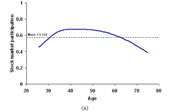
When addressing household investment allocations it is important to distinguish between two distinct decisions: participation and portfolio shares. First, participation represents the binary choice of whether to participate in the stock market or not. Stock market participation in the US is currently just above fifty percent: Bertaut and Starr-McCluer (2002) report that 56.9% of American households hold risky assets.8 There is a clear age effect on participation, and a hump shape in the age profile of people who hold risky assets has been much discussed (Alan, 2006; Ameriks and Zeldes, 2001; Poterba and Samwick, 1997; Gomes and Michaelides, 2005). The top panel in figure 1 uses data from the US Survey of Consumer Finances on stock market participation.9 We see limited participation at early and late stages of life, with a peak around age forty-five. This clearly details the hump shape discussed in the literature. Participation is also increasing in wealth, with richer households much more likely to hold risky assets than poorer households. Using multivariate probit techniques, Bertaut and Starr-McCluer (2002) find that both age and wealth effects are significant for the participation decision in the US. Interestingly, there is substantial turnover in this set of participants, with many people moving both in and out of the stock market. Vissing-Jorgensen (2002) estimates an extremely high turnover rate of around 28% for households with positive wealth, with exit accounting for a substantial portion of those changing participation status.10
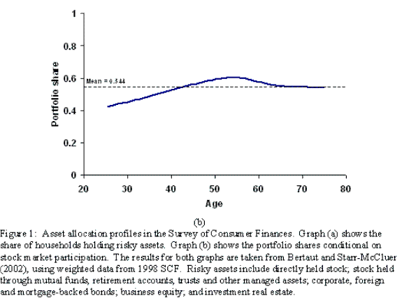
The second important asset allocation statistic is the portfolio share. This represents the share of risky assets to total assets, conditional on participating in the stock market. These portfolio shares are documented to be well below 100% for almost all individuals (Ameriks and Zeldes, 2001; Bertaut and Starr-McCluer, 2002; Gomes and Michaelides, 2005; and others). Bertaut and Starr-McCluer (2002) find that the average portfolio share of stock market participants in the US is 54.4%.11 The bottom panel of figure 1 shows a fairly flat age profile, indicating that portfolio shares do not vary substantially over the life-cycle. Some decline can be seen after retirement, which is consistent with financial advisors recommending clients to shift their portfolios away from risky assets as they age.12 However, econometric studies tend to find that age effects are not significant (see, for example, Bertaut and Starr-McCluer, 2002).
The model in this paper is calibrated to match these three average statistics (asset holdings, participation and shares), explaining the limited participation and strong portfolio diversification seen in the data. As a robustness check for our model's success, we also seek to account for the age profiles of these statistics (particularly that of participation given its documented empirical significance) and ask whether we can explain some of the turnover in stock market participants.
3 Life-Cycle Model
Individuals are assumed to maximize the sum of expected discounted lifetime utility in light of uncertain and uninsurable labor income and rate of return risk. Utility is defined over a single nondurable consumption good, and is additively separable across time. Let there be ![]() periods in the life-cycle, of which a given
periods in the life-cycle, of which a given ![]() periods are spent in retirement and
periods are spent in retirement and ![]() give the working life. This standard set-up gives the following constrained maximization problem:
give the working life. This standard set-up gives the following constrained maximization problem:
![\displaystyle \max_{\omega_{s},C_{s}}E_{t}\left[ \sum_{s=t}^{T}\beta^{s-t}u(C_{s})\right]](img6.gif) |
(1) |
subject to,
during working life (
during retirement (
We impose the terminal condition
![]() . In each period
. In each period ![]() is the discount factor;
is the discount factor; ![]() is consumption;
is consumption; ![]() is the amount of assets held at the start of period
is the amount of assets held at the start of period ![]() ;
; ![]() is the portfolio share; and
is the portfolio share; and ![]() is exogenous real disposable labor income net of taxes. During working life, labor income is uncertain
and non-diversifiable and is taxed at a proportional rate of
is exogenous real disposable labor income net of taxes. During working life, labor income is uncertain
and non-diversifiable and is taxed at a proportional rate of ![]() :13
:13
| (4) |
Following MaCurdy (1982), Abowd and Card (1989), and Moffitt and Gottschalk (2002), we assume that the labor income process can be broken down into a deterministic component and two stochastic components, a permanent and a transitory shock:14
| (5) |
where
| (6) |
Both transitory and permanent shocks are assumed to be independently and identically distributed lognormally such that
![]() and
and
![]() . The income process is truncated such that a zero level of income cannot be realized.
. The income process is truncated such that a zero level of income cannot be realized.
For the final ![]() periods of life, individuals are retired, during which time they receive a constant and certain pension income,
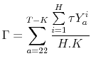
periods of life, individuals are retired, during which time they receive a constant and certain pension income, ![]() . We construct a pay-as-you-go pension scheme, somewhat akin to the arrangements in the US, with pension payments being funded out of contemporaneous tax revenues.15 Allowing for the tax collection requirement of public pension provision is new to the literature on household portfolios.16 Let us assume that an economy is made up of H individuals. At any particular point in time, we assume that there exists an equal mass of individuals at each age; with working population share being
. We construct a pay-as-you-go pension scheme, somewhat akin to the arrangements in the US, with pension payments being funded out of contemporaneous tax revenues.15 Allowing for the tax collection requirement of public pension provision is new to the literature on household portfolios.16 Let us assume that an economy is made up of H individuals. At any particular point in time, we assume that there exists an equal mass of individuals at each age; with working population share being
![]() , and the fraction of households in retirement given by
, and the fraction of households in retirement given by
![]() . Tax revenue collected from individual
. Tax revenue collected from individual ![]() at age
at age ![]() is given by
is given by
![]() . Summing pension contributions over all individuals,
. Summing pension contributions over all individuals, ![]() , and all
working ages,
, and all
working ages, ![]() , and normalizing by the number of retirees,
, and normalizing by the number of retirees, ![]() , gives the
following constant annual pension income for each retired household:17
, gives the
following constant annual pension income for each retired household:17
 |
(7) |
We assume the portfolio investment is composed of two distinct saving tools, a riskless and a risky asset, with
![]() representing the share of assets held in risky forms. The riskless asset has a constant real return of
representing the share of assets held in risky forms. The riskless asset has a constant real return of ![]() and the risky asset has a stochastic real return of
and the risky asset has a stochastic real return of
![]() , with shocks to the excess return assumed to be independently and identically distributed:
, with shocks to the excess return assumed to be independently and identically distributed:
| (8) | ||
We do not impose any correlation between stocks and labor income as the empirical evidence on the size and magnitude is mixed. Heaton and Lucas (2000) find insignificant estimates for all but the highest educational group, and Davis and Willen (2000), surprisingly, find negative correlations for low educational groups. Further, the effect of such a correlation has been shown to make very little difference to participation and portfolio shares in practice (Gomes and Michaelides, 2005), unless unrealistically high correlation coefficients are chosen.
In order to invest in risky assets, in any given period, we assume an individual has to pay some fixed cost. It is clear that gathering and processing financial information plays an important role in investment decisions: acquiring data on financial markets, monitoring brokers, and keeping up to
date with trends, all take considerable time. These financial decisions must be made at each and every point when an individual invests in stocks, implying that any relevant information costs must be considered on a per period basis. In addition to these information costs, holding stocks leads to
substantially more complicated annual tax returns. In the US, households investing in risky assets must fill out schedules D and D1, which take considerable time to complete. Econometric studies by both Paiella (2001) and Vissing-Jorgensen (2002) have asserted the empirical significance of such
fixed costs paid in each and every period of stock market participation. We denote these fixed time costs by ![]() , and we include them in the asset evolution equations ([2] and [3]) scaled by the permanent component of labor income,
, and we include them in the asset evolution equations ([2] and [3]) scaled by the permanent component of labor income, ![]() .18 This scaling follows from the motivation of these costs representing opportunity costs of time: richer households have to forego greater earnings while spending time filling out their schedule D and D1 than poor households. The
fixed costs are interacted with an indicator function,
.18 This scaling follows from the motivation of these costs representing opportunity costs of time: richer households have to forego greater earnings while spending time filling out their schedule D and D1 than poor households. The
fixed costs are interacted with an indicator function,
![]() , which is equal to one for every period of participation and zero otherwise.
, which is equal to one for every period of participation and zero otherwise.
Some limited borrowing is allowed, up to the discounted sum of the minimum income individuals will receive in each remaining period, with no borrowing permitted against pension income. A short sales constraint is imposed on equity such that the portfolio shares must always lie between zero and one (inclusive). Therefore, agents can only borrow at the risk free rate and can only invest in risky assets if they hold positive balances.19
This set-up gives us a system with three state variables (
![]() ) and two control variables (
) and two control variables (
![]() ). The first order condition of the value function with respect to consumption is given by:
). The first order condition of the value function with respect to consumption is given by:
and the first order condition with respect to portfolio share is given by:
These two conditions can be solved for the following policy functions in each period:
| (11) |
| (12) |
These two optimal decision rules are solved recursively from the final period for a discrete number of points in the state space. The details of the solution method are given in Appendix A.
4 Simulation Results
Once the optimal policy functions have been determined, we can simulate the model to imitate the behavior of a population of households and report average allocations to show the effect of introducing fixed costs and changing the public pension scheme. Initially, we detail the functional forms, parameter values and calibration statistics used. Then we show the results of simulating the model for 10,000 ex-ante identical households who differ in the realization of shocks and their initial wealth.
We put forward the results in four subsections: first, we analyze the effect of introducing per period fixed costs to our baseline life-cycle model, and show that this modification changes the participation results substantially. Second, we illustrate the effects of altering the generosity of public pensions, and explain the link between pension generosity and the calibrated level of fixed costs. Third, we calibrate the coefficient of risk aversion, and demonstrate how our model is able to match both participation and shares. Finally, we detail the effect of including a small possibility of a stock market crash, and argue that this enables us to explain all key financial statistics. This structure permits us to disentangle the different consequences of varying fixed costs, public insurance and return risk in order to better fit the model to the data.
4.0.0.1 Parameters and Calibration
The utility function is assumed to take the typical constant relative risk aversion (CRRA) form:20
 |
(13) |
with a baseline value of 2 for the coefficient of risk aversion. This is in line with estimates based on consumption data: Attanasio and Weber (1995) estimate the coefficient of risk aversion to be around 1.5, Gourinchas and Parker (2002) estimate risk aversion to range from 0.28 to 2.29, and Alan and Browning (2003) find ranges from 1.2 to 1.95.
The riskless rate of return is set at a constant value of 1.6%, which represents the average annualized real rate of US 3-month treasury bills from 1960-2000. The risky return is drawn from a distribution with a mean of 5.6%, corresponding to a 4% equity premium,21 and a standard deviation of 0.2.22
Following Haliassos and Michaelides (2003) we set the deterministic trend of income, ![]() , to 3%. Standard magnitudes for the variance of permanent and transitory shocks to income are used. We
take the values directly from Gomes and Michaelides (2005), which are very similar to those used by Gourinchas and Parker (2002) and Carroll (1997). All exogenous parameters are shown in table 1.
, to 3%. Standard magnitudes for the variance of permanent and transitory shocks to income are used. We
take the values directly from Gomes and Michaelides (2005), which are very similar to those used by Gourinchas and Parker (2002) and Carroll (1997). All exogenous parameters are shown in table 1.
The baseline tax rate of 30% gives a retirement replacement rate of 45% of final working period labor income. In reality, the pension tax system in the US is more complicated than the set-up assumed here, but this proportionate rate is chosen as a reasonable proxy. The implied replacement ratio is in line with those used in the literature, for example, Low (2005) used a 55% replacement rate.
The values for the fixed cost, discount rate and (in the final three scenarios) risk aversion are chosen by calibration.23 The value of the fixed cost is chosen to match simulated mean participation with the observed mean in the data (0.57). We choose the discount rate such that simulated ratio of median assets to median incomes matches the data for the working households (1.84).24 Additionally, in the final three scenarios, we choose the risk aversion parameter to match the mean portfolio share statistic of 0.54. Calibration parameters and statistics are shown in table 2.
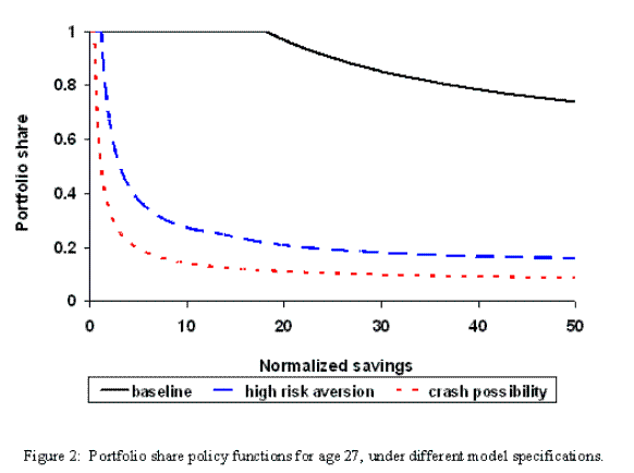
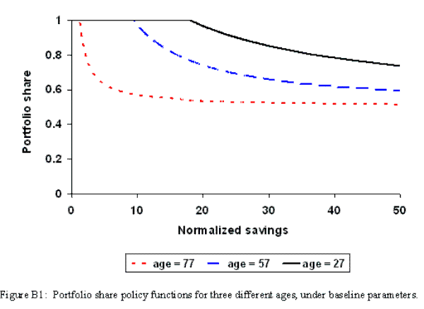
At this point, it is important to point out that one of the main contributions of this paper is to emphasize the importance of matching asset holdings. In these household models both participation and portfolio shares are highly sensitive to the level of assets. Many of the studies claiming to explain certain features of asset allocations implicitly rely on counterfactual asset holdings for their results. To understand the importance of asset levels the solid line in figure 2 plots the portfolio share policy function for an individual of age 27 under our baseline parameters.25
Studies such as Gomes and Michaelides (2005) are able to obtain reasonable portfolio shares by allowing asset holdings to be unrealistically high. This pushes households onto the non-linear sections of their portfolio share policy functions (positioned on the solid line towards the far right in figure 2), enabling movements away from complete specialization in risky assets. In contrast, studies claiming to be able to match participation (Alan, 2006) achieve this by forcing assets down to levels where the borrowing constraint often binds. In fact, in these models non-participants are implicitly assumed to be those hitting their borrowing constraints. With such low amounts of saving, agents are operating on the horizontal section of their portfolio share policy functions (positioned on the solid line close to the y-axis in figure 2), hence these authors find very high shares, typically unity. In this paper we ensure a more genuine matching of asset allocations by explicitly calibrating our model to the actual level of assets observed in the US.
4.1.0.1 Standard Model without Fixed Costs
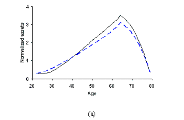
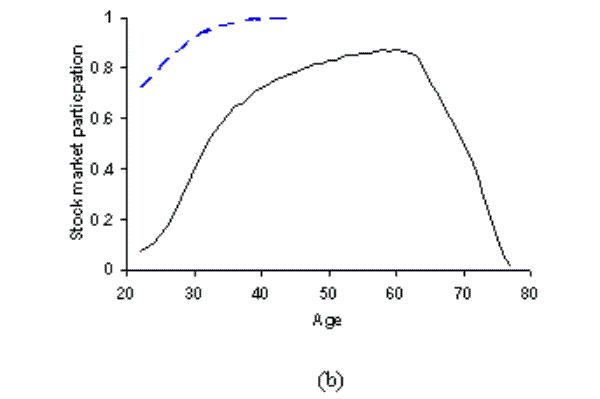
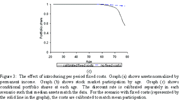
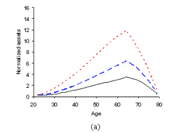
In our initial parameterization we set the per period fixed costs to zero and calibrate the model to match the PSID median asset to income ratio over working life (1.84). The dashed-line graphs in figure 3 show the cross-sectional mean profiles of normalized asset holdings,26stock market participation and conditional portfolio shares.
Under the baseline parameters the discount rate (![]() ) necessary to match the level of assets is 0.5%, giving a discount factor
) necessary to match the level of assets is 0.5%, giving a discount factor
![]() . This high calibrated discount factor results from the high effective impatience introduced with our public pension scheme. The high tax, and subsequent high pension payments,
increases the steepness of disposable income growth requiring only a modest
. This high calibrated discount factor results from the high effective impatience introduced with our public pension scheme. The high tax, and subsequent high pension payments,
increases the steepness of disposable income growth requiring only a modest ![]() to keep savings at the required level. The dashed line in the top panel of figure 3 shows agents
accumulating assets up until retirement, and then running their balances down during the last 15 years of non-working life, reaching levels that are in the same order as those seen in the data (Low, 2005). Average assets are always positive, but some individuals do borrow, up to the endogenous
borrowing limit, in the early stages of life.
to keep savings at the required level. The dashed line in the top panel of figure 3 shows agents
accumulating assets up until retirement, and then running their balances down during the last 15 years of non-working life, reaching levels that are in the same order as those seen in the data (Low, 2005). Average assets are always positive, but some individuals do borrow, up to the endogenous
borrowing limit, in the early stages of life.
The dashed line in figure 3(b) shows that participation in the stock market is 100% for all but a few years in early and late life, and only those individuals with negative savings do not participate. This is in conflict with the data, clearly illustrating the famous ![]() portfolio participation puzzle", discussed at length in the household finance literature. Moreover, in the absence of transactions costs there is no explicit participation decision;
nonparticipants are simply those agents in debt, who are constrained not to hold risky assets by the bounds on
portfolio participation puzzle", discussed at length in the household finance literature. Moreover, in the absence of transactions costs there is no explicit participation decision;
nonparticipants are simply those agents in debt, who are constrained not to hold risky assets by the bounds on
![]() . Turnover is extremely low at 0.5%,27
and this is dominated by households entering the stock market rather than exiting. Figure 3(c) details portfolio shares of stock market participants, and these are high across the life-cycle. The mean portfolio share is 0.99 which is well above the actual value of 0.54. These results exemplify the
inability of the standard framework to explain household asset allocations at reasonable wealth levels: neither participation nor shares are close to being matched.
. Turnover is extremely low at 0.5%,27
and this is dominated by households entering the stock market rather than exiting. Figure 3(c) details portfolio shares of stock market participants, and these are high across the life-cycle. The mean portfolio share is 0.99 which is well above the actual value of 0.54. These results exemplify the
inability of the standard framework to explain household asset allocations at reasonable wealth levels: neither participation nor shares are close to being matched.
4.1.0.2 Including Per Period Fixed Costs
Introducing market frictions, and calibrating the model to match the asset to income ratio of 1.84, leads to a slightly lower discount rate (from 0.5% to 0.3%).28 These per period fixed costs increase the cost of saving, and so the discount rate must fall to keep the level of savings constant. The level of the per period fixed cost is calibrated to match the average participation rate of 0.57, giving a value of 4.6% of the permanent component of labor income. The age profiles are detailed in the solid lines in figure 3. We can see that the increased cost of saving depresses asset accumulation early in life. This reduced precautionary saving is compensated by more retirement saving in mid-life, in order to keep the median asset level calibrated to 1.84.
The introduction of per period fixed costs has a marked effect on the stock market participation profile, with a clear hump shape now evident in figure 3(b). Few individuals accumulate sufficient wealth in the first ten years of working life to make it viable to pay the fixed costs of participation, and they hold only riskless assets in their portfolio. As individuals age they accumulate assets, risky investments become profitable and participation increases - peaking at age 60 with 87% participation. As assets are drawn down later in life, the number of individuals participating is seen to fall gradually back to very low levels. It is important to note that we are not calibrating the model to match the participation age-profile, but we obtain a clear hump shape in all simulations incorporating per period fixed costs.
We see much greater turnover in participation, with the rate increasing twelvefold to 5.5% when per period fixed costs are included. As these costs must be paid during each period of participation we are able to explain exit from the stock market, as well as entry. A bad realization of labor income may drive down the wealth of stock market participants to levels where it is no longer worth paying the fixed cost, and these agents will exit the stock market. The addition of per period fixed costs enables the life-cycle model to explain exit from the stock market for agents with positive wealth. In previous work, households only left the stock market when wealth hit their borrowing constraint, which is unconvincing given the empirical evidence of many households exiting with positive wealth holdings. However, our turnover rates do not reach the high levels documented by Vissing-Jorgensen (2002), though this may be partly due to differing definitions for turnover.29
These fixed costs ensure that stock market participants endogenously hold greater levels of savings, generating a more pronounced age profile in the conditional portfolio shares - as evident in figure 3(c). However, the model continues to predict complete specialization in risky assets early in life with a mean portfolio share of 0.98,30 which is considerably higher than observed in the data.
4.2 Changing the Generosity of the Public Pension Scheme
In this section we analyze the effect of changing the public pension generosity in a model where fixed costs are calibrated to match the US average participation in the stock market. The public pension scheme we have introduced is a form of forced-saving, and varying the generosity of provision will lead to different levels of voluntary saving and stock market participation. Lowering the tax rate leads to less pronounced income growth over the working life and smaller state pension payments during retirement. At a given set of preference parameter values, this lower effective impatience will lead to greater amounts of precautionary and retirement savings.31 In this scenario we hold the discount rate constant, at the level calibrated in section 4.1, while varying the tax rate. We calibrate the per period fixed costs to match average participation.
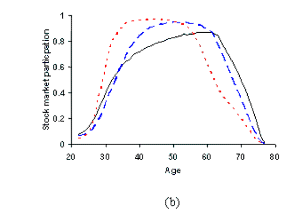
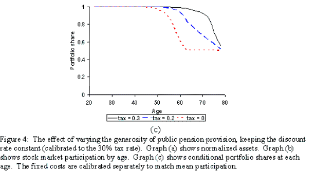
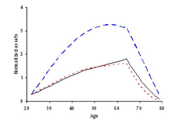
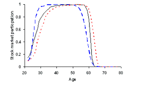
We find that reducing the generosity of the public pensions scheme has a significant effect on the required level of fixed costs: increasing from 4.6% (when the tax rate is 30%), to 7.1% (when the tax rate is 10%), to 10.7% (when the tax rate is zero). In figure 4(a) the crowding out effect of our forced-saving public pensions is clearly evident. Reduced public pension provision is compensated for by greater private retirement savings, leading to very rapid wealth accumulation over the working life. This increased saving allows earlier initial entry to the stock market and higher participation rates during mid-life. Smaller tax rates lead to more diversification of assets; however, shares remain unrealistically high at early stages of life, and mean shares are substantially above their true value (see table 2).
This scenario demonstrates a number of important issues. First, households accumulate assets too rapidly in the absence of public pensions. Second, the hump shape in the age profile for participation is too pronounced for low levels of pension provision. Finally, fixed costs are negatively related to the intensity of public insurance. This final point implies that the small empirical estimates of these fixed costs should not be surprising.32 Given the well developed social security system prevalent in the US, households hold modest retirement savings and only a small fixed cost is required to explain the observed limited participation.
4.3 Calibrating Risk Aversion
The above scenarios demonstrate how restricting ourselves to plausible participation and asset holdings lead to excessively high portfolio shares. This trade off between participation and shares has been well documented in the household finance literature. With the standard model specification, the structure of power utility dictates that large diversification can only take place if savings are substantial (see the policy function depicted in the solid line in figure 2). However, when savings are large, households are highly motivated to participate; making it impossible to reconcile limited participation with small portfolio shares. Our per period fixed cost extension enables us to break this trade off, and match both features within one model.
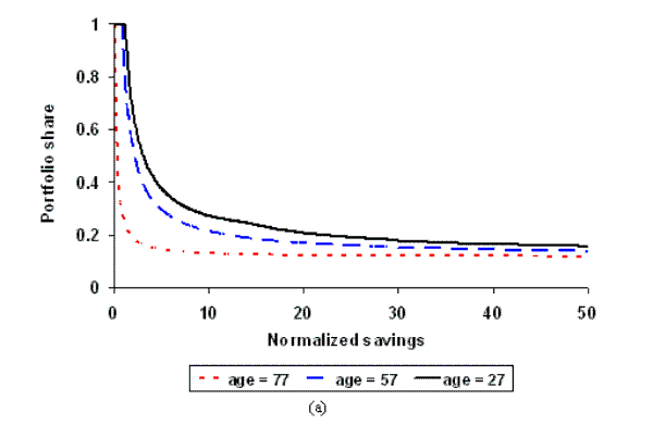
The shapes of the portfolio share policy functions are determined to a large extent by the degree of risk aversion.33 Furthermore, the absolute lower bound of these functions is governed by this parameter through the Samuelson rule.34 The difficulty in matching shares stems from the fact that low risk aversion, as advocated by econometric studies on consumption, leads to a very high value for this lower bound. Under our baseline parameters, this lower bound for portfolio shares is 0.5. Given such diversification is only reached as savings go to infinity, we cannot hope to obtain shares of 0.54 at plausible levels of savings.
By increasing the coefficient of risk aversion, we can reduce this lower bound, shifting the policy functions down and inwards towards the origin. This can be seen by comparing the solid and dashed lines in figure 2.35 This identifies a link between risk aversion and shares: for any given level of savings we obtain smaller shares with higher risk aversion. Our model set-up allows us to take advantage of this relationship, and calibrate the risk aversion parameter to match simulated average shares with the data. In this section we detail the results of this calibration in two different scenarios: firstly, keeping the discount rate at our baseline parameterization; and secondly, re-calibrating the discount rate to match actual savings.
4.3.0.1 Matching Participation and Shares
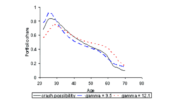
In this scenario we fix the discount rate to the value calibrated in section 4.1. Rather than exogenously set the coefficient of risk aversion, we choose it by calibration such that simulated mean shares match the 0.54 value seen in the data. We calibrate fixed costs to match mean participation as before. The calibrated parameters and simulated statistics are shown in table 2, and the simulated profiles are represented by the dashed line in figure 5.
We obtain a high risk aversion parameter of 9.5 and a per period fixed cost of 2.5% of the permanent component of labor income. Figure 5(b) shows the age profile for participation displaying the expected hump shape. The portfolio share profile in figure 5(c) is now much more realistic, with values well below unity for most of life and declining as households age.36 Thus, we have moved away from the prediction of complete specialization in stocks at young ages. This scenario demonstrates that we are able to match both mean participation and mean shares, within the standard life-cycle framework. However, at this discount rate our asset holdings are very high. This result is comparable to that of Gomes and Michaelides (2005), without requiring preference heterogeneity or non-power utility.
4.3.0.2 Matching Participation, Shares and Wealth
In this scenario our model is shown to match all three key financial statistics. We calibrate the discount rate to match median asset holdings (1.84), risk aversion to match mean portfolio shares (0.54) and per period fixed costs to match mean participation (0.57). The results are detailed in the dotted lines in figure 5.
The age profiles are all reasonable, in particular we have portfolio diversification at all ages - see figure 5(c). Calibrated fixed costs now fall to 1.2% of the permanent component of labor income, which is close to the empirical findings discussed earlier. The calibrated coefficient of risk aversion is high at just over 12. In order to counter this risk aversion, and the entailing high precautionary motive, an uncomfortably large discount rate of 26.2% is required to match asset holdings. Even the high tax rate of 30% cannot moderate impatience at these parameter values.
4.4 Stock Market Crash Possibility
A potential explanation for the model's failure to explain the stylized facts at reasonable preference parameters is risk misspecification. Solving such a dynamic optimization problem involves specifying a subjective probability distribution for the stochastic processes. The standard approach for this involves applying the law of large numbers, and assuming we have sufficient time series of data to substitute past sample moments for future population moments. If data are drawn from a sample which is unrepresentatively tranquil, the law of large numbers may not hold and ex post realized returns will differ from ex ante expected returns. We posit that extreme movements in stock returns are more likely than assumed by the Gaussian distributions and finite sample moments that we tend to use.
Normality is adopted mainly for analytical convenience, and there is now growing debate over the adequacy of such thin-tailed distributions for approximating financial stochastic variables, most vocally by Mandelbrot (1963, 1967, 1997, 2001). Stock returns are subject to many random leaps and jumps, pushing the realized value far from the mean. Examples include the stock market crash of 1987, the collapse of Enron in 2001, the financial crisis of 2008, and to an even greater extent the Great Depression. Solving dynamic programs with discretized normal distributions does not allow for such large departures from the mean, and this is likely to lead to an underestimation of the true risk of holding stocks.
We propose a simple extension to the standard Gaussian framework, whereby we insert a discrete i.i.d. rare disastrous state in the stock market. We assume that such an outcome occurs with a known proportional reduction in returns, and with a known probability. This extension is analogous to the
Carroll (1992, 1997) zero income shock possibility. We set the probability of a stock market crash to 1%, and assume that during the disastrous event households lose all wealth held in risky assets, that is
![]() .37 Our assumed 1% probability
is similar to the probabilities associated with disasters in the related literature on extreme events and the equity premium puzzle (Rietz, 1988; Barro, 2006). However, we are assuming a potential loss of much greater magnitude than any realized during the sample period. Individuals are assumed to
worry about the possibility of the stock market being completely wiped out by a crash, even though no such extreme event has been witnessed: this is an application of the Peso Problem Hypothesis.
.37 Our assumed 1% probability
is similar to the probabilities associated with disasters in the related literature on extreme events and the equity premium puzzle (Rietz, 1988; Barro, 2006). However, we are assuming a potential loss of much greater magnitude than any realized during the sample period. Individuals are assumed to
worry about the possibility of the stock market being completely wiped out by a crash, even though no such extreme event has been witnessed: this is an application of the Peso Problem Hypothesis.
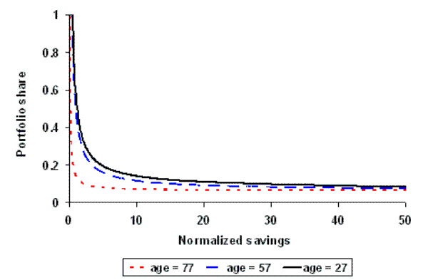
This small probability of a stock market crash has a significant effect on the portfolio share policy functions. The dotted line in figure 2 shows how this extension shifts the policy function further down and inwards towards the origin.38 This enables significant portfolio diversification at low, realistic levels of savings. Under these assumptions, we again calibrate the discount rate, fixed cost and risk aversion parameters to match wealth, participation and shares respectively (as in the previous scenario). The results are detailed in the final row in table 2 and simulated profiles are shown in the solid line in figure 5.
The life-cycle profiles are all reasonable: with assets being accumulated at the correct pace, a hump shape in participation, and portfolio shares being diversified across all ages. We have a 5% turnover rate in stock market participants. The most striking result is on the calibrated parameters, we are now able to match the data at plausible parameter values. A risk aversion of 8.8 is required to enable modest share holdings. This estimate is somewhat higher than suggested by empirical studies using consumption data, however, it remains within the bounds considered reasonable by Mehra and Prescott (1985) and is consistent with the macro finance literature.39 The per period fixed cost is now calibrated to less than one percent of annual labor income, which is closely in line with the empirical estimates of Paiella (2001) and Vissing-Jorgensen (2002). The calibrated discount rate is 9%, which is well within the range estimated by Alan and Browning (2003).
5 Conclusions
In this paper we analyze household saving decisions in the presence of two distinct saving tools and public pension insurance. We are able to match the life-cycle averages of wealth and asset allocations, while keeping to a fairly simple framework with realistic parameter values. It is important to stress that the literature on household portfolios has tended to ignore the matching of wealth, and has focused on matching one asset allocation statistic at a time (participation or shares, but not both). Household models of portfolio choice are very sensitive to the level of wealth, and if we wish to have a coherent explanation of asset allocations we must ensure realistic wealth accumulation.
We demonstrate that a standard portfolio choice life-cycle model, calibrated to match the level of wealth of US households, gives extreme rates of stock market participation and very high portfolio shares. This is at odds with empirical findings, and is the basis for many of the puzzles highlighted in the literature. Introducing per period fixed costs enables us to calibrate the model to match the observed limited participation at actual wealth levels. These costs generate the desired hump-shaped age profile for participation, and help resolve the issue of turnover. We present a stylized pay-as-you-go pension scheme, and show that reasonable pension provision is required to keep the asset accumulation and participation age profiles in line with data.
Our framework allows us to calibrate the model to match both participation and shares, in contrast to previous work which asserted that there must exist a trade-off between matching these two statistics. However, this result comes at some cost, requiring us to accept either high wealth accumulation or high parameter values. Adapting the subjective probability distribution of returns to allow for a disastrous event in the stock market has a considerable effect on our results. We are now able to match all three statistics at reasonable parameter values, without resorting to heterogeneous preferences or moving away from power utility functions. Through our three extensions, we are able to resolve both the "portfolio participation puzzle" and the "portfolio composition puzzle" with a per period fixed cost of 0.8% of annual labor income, risk aversion of 8.8 and discount rate of 9%.
Appendix A: Solution and simulation methods
The results presented in section 4 use standard techniques to solve a life-cycle model by backwards induction. We start from a terminal condition on assets, and obtain the optimal policy functions for each age, which map the state variables into the controls. Using these functions the model is
simulated forward from ![]() with 10,000 ex-ante homogenous individuals who differ in shock realizations. Following Alan (2006), initial assets are drawn from a lognormal distribution, whose
underlying normal distribution has a mean of -3.15 and standard deviation of 1.96. Mean life-cycle profiles of accumulated wealth and asset allocations are then computed.
with 10,000 ex-ante homogenous individuals who differ in shock realizations. Following Alan (2006), initial assets are drawn from a lognormal distribution, whose
underlying normal distribution has a mean of -3.15 and standard deviation of 1.96. Mean life-cycle profiles of accumulated wealth and asset allocations are then computed.
Solving the Euler equations corresponds to the determination of a fixed point within an infinite dimension state space, involving expectations over a non-linear marginal utility function, where the unknown is a function over a continuum of points. Such complexity means that the model cannot be solved analytically, which entails the implementation of numerical techniques. The state space is discretized into a finite number of nodes and interpolated using local approximation methods.40
The grids are defined so as to avoid the need for extrapolation outside the grid.41 The concavity of the consumption function leads us to choose a non-uniform spacing of the asset nodes. Extra points are positioned close to the lower bound, where the consumption policy function displays a significant amount of curvature. The nodes are more spread out at high asset levels, at which point the functions become approximately linear. The savings grid is also non-uniformly spaced as the portfolio share policy function is non-linear. More points are positioned around the kink in the policy function, where the short sales constraint ceases to bind, and fewer nodes at high levels of savings, where the policy function becomes almost horizontal approaching the complete markets outcome. The solution is found using NAG routines,42 except for when these methods fail to converge, in which case the non-linear system is solved using a bisection method.43
We perform all numerical integration using Gaussian quadrature to approximate the distributions of labor income and the risky asset. The income shocks are discretized into six values and the risky return uses three point quadrature. In the simulations, the permanent shock to labor income is
approximated as a continuous random variable. Each time period is taken as a year of life. ![]() is taken to be 58 years and
is taken to be 58 years and ![]() as 15 years, giving a working life of 43 years (from age 22 to 65) and life coming to an end at 80.
as 15 years, giving a working life of 43 years (from age 22 to 65) and life coming to an end at 80.
A check on the accuracy of the solution method is undertaken by computing the realized values of the Euler equations. When averaged across individuals, these results do not deviate substantially from their expected values.
Table 1: Exogenous Parameters
| Parameter | Value |
|---|---|
CRRA ( ) ) |
2 |
| Riskless rate (r) | 1.6 |
Mean risky return (r ) ) |
5.6 |
| Variance of risky return | 0.04 |
Variance of permanent shock (
 ) ) |
0.01 |
| Variance of transitory shock (
|
0.0225 |
| Growth of permanent component of income (G) | 0.03 |
Proportional tax (
 ) ) |
0.3 |
| Tax | Simulated Statistics: Median[Ai,t]/ Median[Yi,t] |
Simulated Statistics: Mean Participation | Simulated Statistics: Mean Shares | Parameters: 1+  |
Parameters: Fixed Costs | Parameters: CRRA | |
| US Data | 1.84 | 0.57 | 0.54 | - | - | - | |
| Scenario: No Fixed Cost | 0.3 | 1.84 | 0.95 | 0.99 | 1.005 | - | 2.0 |
| Scenario: Calibrated Fixed Cost | 0.3 | 1.84 | 0.57 | 0.98 | 1.003 | 0.046 | 2.0 |
| Scenario: Keeping Discount Rate Constant | 0.3 | 1.84 | 0.57 | 0.98 | 1.003 | 0.046 | 2.0 |
| Scenario: Keeping Discount Rate Constant | 0.2 | 2.98 | 0.57 | 0.95 | 1.003 | 0.071 | 2.0 |
| Scenario: Keeping Discount Rate Constant | 0.0 | 4.89 | 0.57 | 0.90 | 1.003 | 0.107 | 2.0 |
| Scenario: Calibrating CRRA | 0.3 | 4.11 | 0.57 | 0.54 | 1.003 | 0.025 | 9.5 |
| Scenario: Calibrating CRRA | 0.3 | 1.84 | 0.57 | 0.54 | 1.262 | 0.012 | 12.1 |
| Scenario: Crash Possibility | 0.3 | 1.84 | 0.57 | 0.54 | 1.090 | 0.008 | 8.8 |
