Financial Market Shocks during the Great Depression
October 22, 2009
Keywords: Financial shock, impulse response, VAR
Abstract:
1 Introduction
Recent events have highlighted the effect of financial system disruptions on the macroeconomy. In a seminal paper, Bernanke (1983) argued that disruptions to the financial system affect the real economy by increasing the cost of credit intermediation. A large subsequent literature has examined this channel with an emphasis on the effect of disruptions to the banking system.1 In addition to bank failures, the Great Depression was also a period of significant financial market stress, which may have contributed to its severity. Motivated by these observation, we present evidence relating financial market shocks to real economic outcomes.2
We examine the effect of shocks observed in financial markets using vector auto-regressions (VARs) on monthly data for output, employment, wholesale prices, and a financial market variable.3 We use the short-run identification method in the analysis with the financial variable ordered last. This captures the effect of an innovation to the financial market variable that is orthogonal to current shocks to productivity, real wages, and nominal prices - all of which have been shown to have played a role during the Great Depression.4 We analyze the effect of financial market shocks using impulse response functions constructed from the VAR estimates. The main contribution of this analysis is to present a detailed analysis on the relationship between shocks observed in financial markets and real economic outcomes in the data.
The financial market variables we use in the study include stock prices, credit spreads, and the total issuance of stocks and bonds. Thus, we measure financial market conditions using both price and quantity data. Although innovations to prices and quantities are correlated, examining then separately enables us to provide a broader picture of the relationship between financial market variables and economic outcomes.
Using this approach, we find that an adverse shock to a financial market variable results in a decrease in manufacturing sector output and total hours. This decrease peaks about 11 months after the shock. Quantitatively, a residual one standard deviation shock to a financial variable leads to a peak output decline of about 3 to 4 percent and a peak total hours decline of about 2 percent. Although our findings can not establish a clear causal relationship, the results indicate a link between shocks observed in financial markets and future manufacturing sector outcomes. The financial market variables accounts for between 10 to 25 percent of the forecast error variance for output and total hours. Cole et al. (2007) find that stock price shocks account for about 25 percent of output variation using a DSGE approach with annual data on a panel of countries from 1929 to 1933.
The theoretical models that underpin our analysis highlight the role of financial markets for financing investment. The agency cost models of Bernanke & Gertler (1989), Carlstrom & Fuerst (1997), and Bernanke et al. (1999) demonstrate that a decline in net worth or an increase in borrowing costs reduces the ability of entrepreneurs to finance investment by lowering their available collateral. Although we do not have monthly data on investment, durables goods sector output provides a good proxy for investment demand. Motivated by this reasoning, we examine whether financial market shocks have a greater effect on the durables goods sector than the non-durables good sector.
We collect new data for the employment and output of the durables and non-durables goods sectors from various Federal Reserve Bulletins. The Federal Reserve Bulletin of August 1940 presents data on industrial output obtained by aggregating output indices across industries. The Federal Reserve Bulletin of October 1938 presents a similar employment series. The data indicate that the durables good sector suffered greater declines during the Great Depression than the nondurables sector, with peak-to-trough declines of output and employment of about 77 and 57 percent, respectively. In comparison, the nondurables sector had peak-to-trough output and employment declines of about 34 and 32 percent, respectively.
VAR analyses on the durables good sector indicate that an adverse shock to a financial variable leads to peak employment and output declines of about 3 and 6 percent, respectively. In comparison, the peak declines for the nondurables sector are all less than 2 percent. This suggests that financial market shocks have a much greater effect on the durables good sector than the non-durables sector, consistent with the investment-channel highlighted in the agency costs literature.5 These results are also consistent with the arguments of Mishkin (1978) and Romer (1989) that declines in net worth exacerbated the Great Depression by lowering the consumption of durable goods by households.
The data indicate that financial market conditions remained weak even while the broader economy was recovering strongly in 1933 and 1934. The stock market declined from July 1933 to December 1934; the average credit spread over these this period was 3.3 percent, compared to 2.3 percent in the period leading up to July 1929; stock and bond issuance reached its lowest point in February 1933 and remained depressed until the spring of 1935. These findings suggest that weakness in financial markets persisted well into the recovery. Combined with our previous results, this indicates that financial market weakness may have contributed to the slow recovery from the Great Depression, as highlighted in Cole & Ohanian (2004). Further evidence of this effect can be seen from the much sharper recovery in the non-durables goods sector as compared to the durables goods sector.
The econometric analysis relates shocks observed in financial markets to real economic outcomes. One clear drawback of this analysis is that it cannot distinguish between a true shock to the financial system and a shock to expectations about future economic outcomes that is observed in the financial system. For instance, the news shock literature - see Beaudry & Portier (2006) - argues that otherwise unexplained stock price movements reflect information about future TFP. However, it is difficult to reconcile this explanation with the continuing financial market weakness observed in the early stage of the recovery from the Great Depression.
If we do capture a shock to the financial system, what may be the underlying structural shock? One possibility is that investors' risk aversion increased following the sharp dislocations associated with the Great Depression (see Cogley & Sargent (2008)). Another possibility is that the Great Depression was associated with a substantial loss of human capital in the financial services industry, leading to an increase in funding costs (see Phillipon & Reshef (2009)). Yet another possibility is that the financial market shocks reflect increases in future uncertainty (see Bloom (2009)). We investigate this last possibility by using stock market volatility, constructed using daily stock return data, as a measure of economic uncertainty. Somewhat surprisingly, we find that including the uncertainty measure has no effect on our results - the negative effect of an increase in uncertainty on the real economy is orthogonal to the effect of a decrease in stock prices.
We also use our estimates from the VAR on the Great Depression to quantify the effect of financial market innovations during the recent financial crisis. We measure the effect of the crisis as the value of financial market innovations during the recent crisis times the impulse response from the VAR on the Great Depression data. This calculation indicates the the sharp declines in stock and bond prices in the fall of 2008, absent further policy interventions, may result in manufacturing sector total hours and output declines of 12 and 16 percent, respectively. Although imprecisely estimated, the findings suggest that adverse financial market shocks during the recent crisis could have a significant negative effect on the manufacturing sector.
This study is organized as follows. Section 2 presents the data employed in the study. Section 3 details the econometric method. Section 4 presents the empirical findings. Section 5 uses the results to examine the effects of the recent financial crisis and Section 6 concludes.
2 Data
This section discusses the data we use in our study. In order of presentation, we discuss the financial market variables, the macroeconomic aggregates, and the sectoral data. The sample period is July 1922 to June 1939. The start date was determined by the availability of data on weekly hours while the end date of the sample was chosen to avoid the effects of World War II.
2.1 Financial market variables
We obtain data on stock prices and credit spreads from the Historical Statistics of the United States Millenium Edition (hereafter, HSUS). We use the Standard and Poor's common stock index from the HSUS (series Cb45) as the stock price series. This series is the precursor to the widely used S&P 500 stock index. In the subsequent analysis, we divide the stock index series by the wholesale price index to translate the stock price into real terms.
We obtain data on Baa-rated corporate bonds (series Cb59), long-term U.S. government bonds (series Cb57), and short-term U.S. government bonds (series Cb56) from the HSUS. The original data source for both interest rates was the U.S. Federal Reserve publication Banking and Monetary Statistics: 1914-1941. The credit spread employed in the study equals the log difference between the Baa bond interest rate and the long-term bond interest rate.
We obtain data on securities issuance from the NBER Macrohistory database. This database contains many series on securities issuance. For the purposes of this study, we use the series titled `Total corporate issues, bonds, notes, and stocks, including refunding, U.S., Canadian and Foreign' as it provides a comprehensive sum of securities issuance in the U.S. capital markets.6
We construct stock market volatility using data on daily stock returns collected by Prof. G. William Schwert. This data is discussed in detail in Schwert (1990). The monthly stock volatility measure used in the study equals the monthly average of the absolute daily stock returns minus the average stock return for that month.
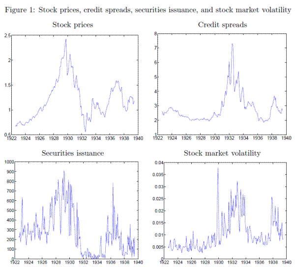
Figure 1 presents the financial variables employed in the study. As is well known, the stock market rose dramatically through the 1920s. It began to decline sharply in the fall of 1929 and reached its lowest point in June 1932. At its trough, the stock market had declined by more than 80 percent from its peak value. Although the stock market improved with the economy, it did not return to its pre-Great Depression peak level until World War II. The path for stock price movements suggests that the attendant sharp decline in net worth may have exacerbated the Great Depression.
Credit spreads exhibit a different path from stock prices during this time period. They remained low in the 1920s amidst the economic expansion. Credit spreads did not begin to rise until the fall of 1930, and then begin a steep climb to above 7.5 percent in May 1932, before beginning to decline to more normal levels. The path for credit spreads suggest that they increased partly in response to adverse economic developments during the Great Depression. However, the sharp rise in credit spreads during 1931 may have worsened the economic downturn.
The data on securities issuance indicate that they increased with stock prices during the boom period in the 1920s. Somewhat surprisingly, securities issuance did not decline sharply until well into the Great Depression. However, it remained very low from 1932 to 1935, even as the overall economy began a strong recovery. This indicates that financial market conditions remained depressed well into the economic recovery, possibly due to a substantial destruction of human capital in the financial services industry.
The stock market volatility series captures the sudden stock market crash in the fall of 1929. Although volatility declined immediately following the crash, it subsequently increased steadily over the downturn and continued to remain elevated until 1934. This indicates that economic uncertainty, as measured by stock price volatility, increased fairly sharply during the Great Depression. Keynes (1936) argues that this increase in uncertainty lead to lower investment and output.
Overall, the figures suggest that financial market weakness may have contributed to the severity of the Great Depression. The impact of sharp stock price declines on net worth and the high real interest rate faced by corporate borrowers would have sharply limited the scope for borrowing during the downturn. Furthermore, continuing financial market weakness in 1933 and 1934 may have restrained the recovery from the Great Depression.
2.2 Macroeconomic data
We obtain data on the wholesale price index and the seasonally adjusted industrial production of manufacturers from various Federal Reserve Bulletins. The industrial production series tracks the quantity produced by manufacturing firms during this time period. We use the wholesale price index because it tracks price changes in the manufacturing sector.
We obtain data on manufacturing employment from the HSUS (series Cb46). This series tracks the employment of production workers in the manufacturing sector. We also obtain average weekly hours of production workers from the HSUS (series Cb48). This series begins in January 1932. We extend this series back using linear interpolation of monthly data on average weekly hours for wage-earners from the HSUS (series Cb49) on annual data on average hours for manufacturing workers from the Employment, Hours, and Earnings, United States, 1909-94.7 In the VARs, we construct total hours as manufacturing employment times weekly hours.
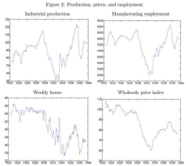
Figure 2 plots these macroeconomic series. The industrial production series highlights the dramatic drop in output during the Great Depression - manufacturing output declined by more than 50 percent from peak-to-trough. Output recovered and reached its trend level by 1937 before declining again in the subsequent downturn. The path for manufacturing sector employment follows the output series, but the peak-to-trough decline for employment is lower than the corresponding drop in output.
The average weekly hours of production workers declined along with output and employment during the Great Depression. This demonstrates that firms adjusted their labor force on both the intensive and extensive margin. The decline in average hours may also reflect pressure on firms to avoid wage cuts.8 Somewhat surprisingly, the weekly hours series remains depressed well into the recovery period. Taken together, the data on output, employment, and hours indicate that labor productivity increased over the 1930s as argued by Field (2003, 2006).
One important feature of the Great Depression was the steep decline in the average price level. The wholesale price index declined by nearly 40 percent from August 1929 to March 1933. In comparison, the consumer price index fell by only about 25 percent, reflecting smaller declines in the price of services such as rent and utilities. The wholesale price index failed to reach its 1920s level until the end of the Great Depression. Such a sharp decline in the price level would amplify financial shocks by increasing the debt burden for outstanding loans.9
2.3 Durable and nondurable goods sectors
The investment-based channel highlighted by the agency cost models of Bernanke & Gertler (1989) and Carlstrom & Fuerst (1997) suggests that financial shocks should have a greater effect on the durables goods sector than the nondurables sector. We collect data on the output and employment of these sectors to examine whether financial shocks had a greater impact on the durables sector.
We obtain data on the output of the durables and nondurables sectors from the August 1940 publication of the Federal Reserve Bulletin. This reports revised index values for monthly output dating back to 1923. The indices were computed as weighted averages of various manufacturing industry groups.
We obtain data on the employment of these two sectors from the October 1938 publication of the Federal Reserve Bulletin. We extended the series to June 1939 using subsequent Federal Reserve Bulletins. The employment indices were also constructed as weighted average of various industry groups.
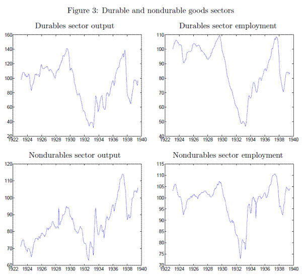
Figure 3 plots the output and employment of these two sectors over the sample period. Output and employment of the durables sector declined steeply over the Great Depression, falling from peak-to-trough by about 77 and 57 percent, respectively. In comparison, the nondurables sector was less affected during the Great Depression, with peak-to-trough declines of output and employment of about 33 percent each. The figures also suggest a much stronger recovery in the output and employment of the nondurables goods sector. The sharper decline and slower recovery of the durables good sector indicate that the durables good sector was more strongly affected during the Great Depression. We subsequently demonstrate that this may be related to adverse developments in financial markets.
3 Empirical method
This section details the empirical method used in the analysis. We use VARs to study the effect of shocks observed in the financial market on output and total hours of the manufacturing sector as well as the durable and nondurable goods sectors. We subsequently discuss the robustness of our findings to changes in the empirical specification.
Each VAR system includes four variables ordered as: the wholesale price index, manufacturing output, manufacturing total hours, and one financial system variable.10 We estimate three separate VARs to separately capture the effect of innovations to stock prices, credit spreads, and securities issuance. We identify the effect of financial system innovations using short-run restrictions.11 As the financial system variable is ordered last, the results capture the effect of shocks observed in the financial system that are orthogonal to contemporaneous shocks to prices, output, and total hours. The inclusion of the price index in the VAR takes into account the effect of monetary shocks during the Great Depression as emphasized by Friedman & Schwartz (1963). And innovations to output and total hours take into account potential productivity shocks and shocks to wage mark-ups during this period.
We use a similar specification for the VAR systems for the durables and nondurable goods sectors. We cannot quite replicate the above analysis due to the lack of separate price indices on each sector and the absence of data on weekly hours for each sector. The sectoral VARs consist of the wholesale price index, sectoral output, sectoral employment, and one financial system variable. The ordering of the VAR is the same as above.
We take log-differences of all variables to ensure stationarity in the VARs. The estimation uses 13 lags in each of the VARs to capture potential deep lags in the system. We check the stability of the VAR coefficients using an eigenvalue test. Using the VAR estimates, we construct cumulative impulse response functions for a residual one standard deviation shock to the financial variable. The figures report these cumulative impulse response over a 24 month period. We use a bootstrap procedure to construct the 95 percent confidence interval for the impulse responses.12
4 Results
This section reports the impulse response functions obtained from the VAR analyses. It also details the various robustness checks we carry out.
4.1 Stock prices
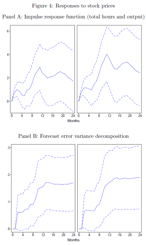
Figure 4 reports the results from the VAR with the real stock price as the financial market variable. Panel A presents the cumulative impulse response function over 24 months for a residual one standard deviation increase in stock prices. Panel B presents the corresponding forecast error variance decomposition.
The impulse responses indicate that an increase in stock prices is followed by an increase in the manufacturing sector's total hours and output. Total hours and output increase by about 1 percent a few months after the impulse. The peak response occurs about 11 months after the impulse - at the peak total hours and output have increased by about 3 and 4 percent, respectively. These increases are statistically and economically significant. Note that although the impulse response of the change in total hours and output fades after 12 months, the cumulative impulse response, shown here, does not fade.
The forecast error variance decompositions indicate that stock price innovations account for about 5 percent of the forecast variance in output and total hours after 3 months. The variance contribution increases to a little under 20 percent after 12 months.
These findings indicate that, consistent with the agency cost models of financial shocks, a stock price innovation affects output and total hours in the manufacturing sector. Furthermore, the impulse peaks with a noticeable lag, as would be the case if the stock price innovation propagates through an investment channel. Beaudry & Portier (2006) present a related finding using more recent data. They argue that stock price changes capture the arrival of news about future TFP. However, given the magnitude of the stock price changes during the Great Depression, it is debatable whether these changes reflect the arrival of news about future productivity. A news shock interpretation would also be inconsistent with the findings of Field (2003) that the 1930s was a decade of rapid productivity growth.
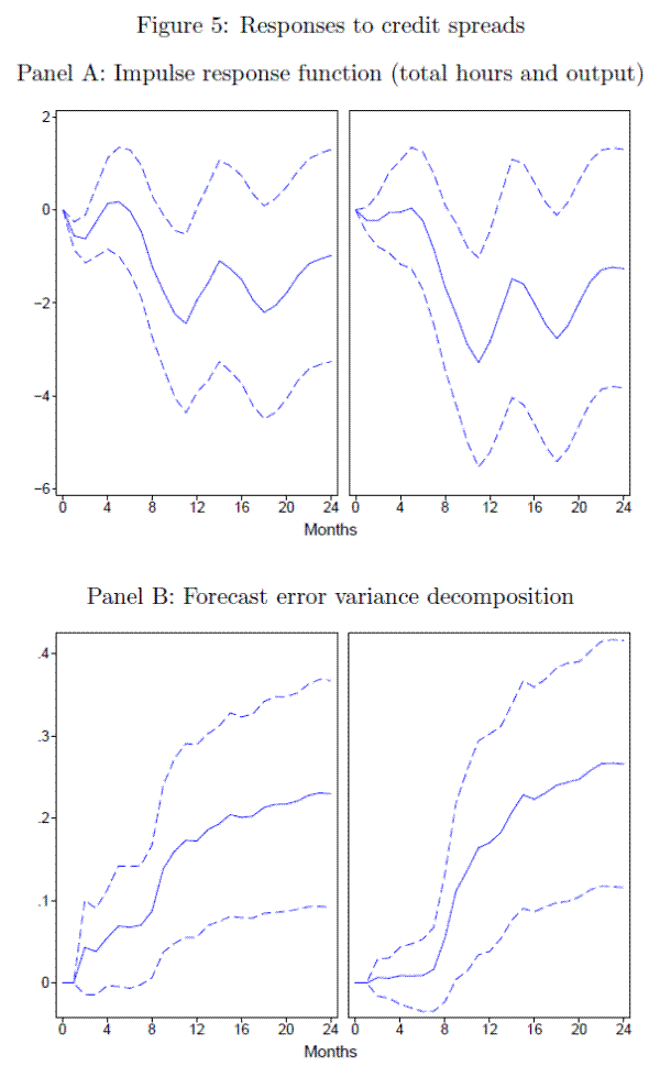
4.2 Credit spreads
Figure 5 reports the results from the VAR with the credit spread as the financial market variable. Panel A presents the cumulative impulse response functions and Panel B presents the forecast error variance decompositions.
The impulse responses show that total hours and output decline following an increase in credit spreads. The peak declines of 2 and 3 percent, respectively, occur about 11 months afterward, similar to the response to stock price innovations. The similarity in the impulse response reflects the high correlation between innovations to stock prices and credit spreads from August 1929 onward.13 However, total hours and output respond much less in the months immediately following an innovation to credit spreads. The forecast error variance decomposition attributes more than 20 percent of the forecast variance in total hours and output to shocks observed in credit spreads.
As with the results in the previous section, these findings are consistent with the main implications of the agency cost models of financial shocks. An increase in the cost of obtaining credit leads to a lagged negative effect on output and total hours. However, we cannot eliminate the possibility that these results reflect changes in expectations about future economic outcomes.
4.3 Securities issuance
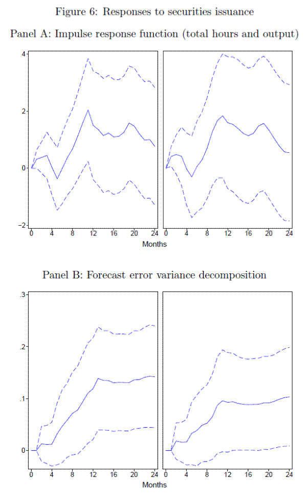
Figure 6 presents the findings from the VAR with total securities issuance as the financial market variable. Panel A presents the cumulative impulse response functions and Panel B presents the forecast error variance decompositions.
The impulse responses indicate that an innovation to securities issuance is followed by an increase in the output and employment of the manufacturing sector. The impulse response peaks about 11 months afterward, similar to that observed with stock prices and credit spreads. Although the total hours peak response is significant at the 95 percent level, the output response is not significant. The results indicate that an improvement in financial markets, as measured by the quantity of securities issued, leads to a lagged improved in manufacturing sector outcomes. Given that a major purpose for issuing securities is to finance investment, these findings are consistent with the investment channel highlighted in the agency costs literature. Although we can not exclude the possibility that our results capture changes in expectations, the very low levels of securities issuance observed in the early stage of the economic recovery from the Great Depression casts doubt on this alternate explanation. As before, the forecast error variance decomposition attributes a significant portion of the variation in output and employment to financial market shocks.
The correlation between changes to stock prices and securities issuance over the sample period is only -0.02. This indicates that the impulse responses obtained with the securities issuance series is not merely a replication of the results obtained with stock prices.
4.4 Durable and nondurable goods sectors
We next examine whether innovations in financial markets have a stronger impact on the durable goods sector than the nondurables sector. Purchases of durable goods by firms and households are often financed by borrowing. Thus, a financial shock would be expected to have a greater effect on the durables sector, consistent with the investment-channel highlighted in the agency costs literature.
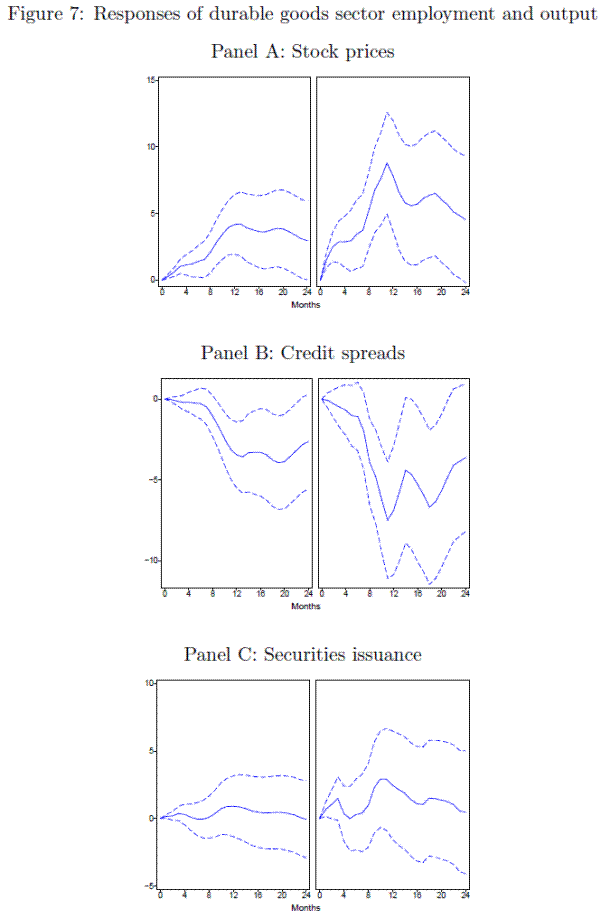
Figure 7 plots the results from the VARs on the durable goods sector. Panels A, B, and C present the cumulative impulse response function over 24 months obtained using stock prices, credit spreads, and securities issuance as the financial market variable, respectively. The sample period extends from January 1923 to June 1939.
The impulse responses indicate that financial market price innovations have a marked effect on the durables goods sector. A one standard deviation increase in stock prices leads to employment and output increases of 4 and 9 percent, respectively. The corresponding impulse responses for innovations to credit spreads equals 3 and 7 percent, respectively. These peak impulses are statistically significant, and substantially larger than those observed for the manufacturing sector as a whole. However, securities issuances leads to a weaker impulse compared to that for stock prices and credit spreads.14
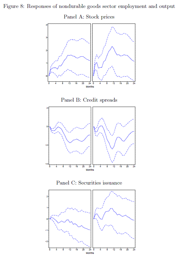
Figure 8 plots the corresponding results from the VARs for the nondurable goods sector. The impulse responses to stock prices and credit spreads for this sector have a similar profile as those the durables sector.15However, the impulse responses for the two sectors are of different orders of magnitude. The peak responses for employment and output in the nondurables sector barely exceed 2 percent. Similar to the durables sector, innovations to securities issuance have no significant effect on the nondurables sector.
Taken together, these results indicate that shocks observed in financial markets have a much greater impact on the durables good sector. This finding is consistent with the investment-based channel emphasized in the agency costs literature. A shock to the marginal efficiency of investment highlighted by Justiniano et al. (2008) would also generate a similar disparate impact on the durables sector. However, the micro-foundations for an investment shock during the Great Depression are unclear, whereas a financial market shock may reflect a shock to risk premia or human capital in the financial services sector.
Section 2.1 documented that financial market conditions remained depressed in late 1933 and 1934. The above results imply that this continuing weakness in financial markets contributed to the very slow recovery in the durables sector documented in Section 2.3. This finding suggests that increased funding costs due to financial market weakness hindered the recovery from the Great Depression.
4.5 Robustness
The analysis presented in the study employed the financial market variables one at a time. We replicate our analysis including stock prices, credit spreads, and securities issuance in the VAR. The resulting impulse responses depend somewhat on the ordering of the financial variables. For all six specifications, innovations to stock prices have a significant effect on output and employment, though the effect varies in strength. The impulse response to innovations to securities issuance have a similar profile, though they cease to become statistically significant when securities issuance is ordered after stock prices. The impulse response to credit spreads depends on whether it is ordered before or after stock prices. An impulse to credit spreads that is orthogonal to stock prices has no clear effect. The impulse response is similar to that reported in Section 4.2 when the ordering is reversed.
We examine the robustness of our results to changes in the empirical specification over a range of other dimensions. Changing the ordering of the non-financial variables over the five other possible permutations has no effect on the results. We also change the number of lags in the VARs from 13 to 7, 10, or 16. We obtain similar results as before with 10 or 16 lags. However, our results change when we use only 7 lags: the impulse response to stock prices peaks after a few months and we no longer find a significant effect for impulses to credit spreads or securities issuance. This change reflects the effect of the deep lags in the VAR system. We also add the short-term interest rate on U.S. treasuries as an additional variable in the VAR system. This has no effect on the impulse response for stock prices. However, the impulse response to credit spreads now has two peaks - one after 11 months and another after 18 months. In general, the robustness checks for the comparison between the durable and nondurable goods sectors follow a similar pattern to that observed for the manufacturing sector.
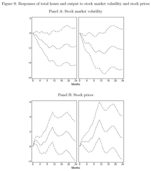
Another possibility we examine is whether our financial market impulses are reflecting increases in uncertainty. We use stock market volatility constructed from daily stock returns as a measure of uncertainty. Figure 9 presents the impulse responses from a VAR with the wholesale price index, manufacturing output, manufacturing total hours, stock market volatility, and stock prices. The impulse response for stock prices is little changed from Figure 4. This indicates that the stock price effect we capture does not reflect a change in uncertainty about the future economy. Interestingly, an increase in uncertainty also has a negative effect on manufacturing sector output and total hours as argued by Bloom (2009) and Bloom et al. (2009).
The results reported in this study were obtained using VARs with log-differences of the non-stationary variables. An alternate approach involves estimating the systems using vector error correction (VEC) models on the levels data. We repeat the analysis using VEC models with the the number of co-integrating equations varying with the variables in each system. We obtain similar impulse response profiles using the VEC as those obtained with the VAR. However, the VEC results attribute a greater share of the forecast variance to stock prices and a lesser share to credit spreads than the corresponding VAR estimates. As before, we find a much stronger impulse for the durables good sector than the nondurables sector.
We examine whether the financial variables used in the study Granger cause output and employment. We find that stock prices and credit spreads Granger cause output and employment for the manufacturing sector as a whole as well as the durables and nondurables sectors; Securities issuance Granger causes manufacturing sector output but not total hours.
5 Effect of recent financial market disruptions
We next use the results from the VARs during the Great Depression to study the effect of financial market shocks during the fall of 2008.16 As detailed in Swagel (2009), financial markets were subject to a series of unexpected events during this period, which lead to sharp adverse movements in stock prices and credit spreads. The previous results suggest that these shocks may have a significant impact on the real economy.
We quantify the effect of the recent financial market shocks using a simple, albeit arguable, approach. We construct fitted values for financial market variables for 2008 using point estimates from the corresponding VARs estimated on the Great Depression data. The realization of each financial market variable minus the corresponding fitted value yields an estimate of financial market innovations. The estimated effect of these innovations equals the financial market innovation times the corresponding impulse response from the VAR on the Great Depression data. This calculation quantifies the effect of these financial market innovations absent other shocks or policy interventions. Thus, the results can not be viewed as a forecast for either output or employment. However, this method does provide a metric to gauge the intensity of the financial market disruptions during fall 2008.
Table 6 presents the estimated effect of financial market innovations during September and October, 2008. The estimated effect on output and employment are reported at the peak impulse response period of 11 months and further on at 18 months. The results indicate that the financial market disruptions are estimated to have an economically large effect on the manufacturing sector, absent further policy interventions.17 At the peak, these innovations are estimated to result in output and total hours declines in the manufacturing sector of about 16 and 12 percent, respectively. The estimated effects for the durable goods sector are even greater, reflecting the larger impulse response values. The wide confidence intervals around the estimates for both sectors reflect the high degree of uncertainty entailed in such a calculation.
6 Conclusion
This study examines the effect of shocks observed in the financial markets on the output and employment of the manufacturing sector. We find that an adverse shock in financial markets leads to lower output and employment, with the peak effect occurring about 11 months afterward. We also document that adverse financial market shocks have a much greater effect on the durables sector than the non-durables sector. Although our method cannot attribute a causal link, these findings are consistent with the agency cost models of financial shocks, where increased borrowing costs lead to reductions in future output and employment.
Although our results pertain to the Great Depression, they may be of some value for thinking about the ongoing recession. Romer (2009) compares the financial strains and policy responses during the Great Depression and the current recession. If a similar relationship holds, our findings suggest that, absent policy interventions, the financial market stress in the fall of 2008 could have had a significant negative effect on the economy in 2009 and beyond.
Bibliography
Journal of Money, Credit, and Banking 37:753-773.
American Economic Review 96:1293-1307.
American Economic Review 73:257-276.
American Economic Review 79:14-31.
In J. B. Taylor & M. Woodford (eds.), Handbook of Macroeconomics, pp. 1341-1390. Elsevier, Amsterdam, The Netherlands.
Econometrica 77:623-685.
Stanford University working paper.
American Economic Review 90:1447-1463.
American Economic Review 87:863-883.
American Economic Review 93:937-947.
Journal of Political Economy 117:165-210.
American Economic Review 87:893-910.
Northwestern University working paper.
Journal of Monetary Economics 55:454-476.
Federal Reserve Bank of Minneapolis Quarterly Review 23:2-24.
Journal of Political Economy 112:779-816.
Working paper, University of Pennsylvania.
American Economic Review 93:1399-1413.
Journal of Economic History 66:203-236.
Econometrica 1:337-357.
Princeton University Press, Princeton, NJ.
Forthcoming, Journal of Monetary Economics.
Federal Reserve Bank of Chicago working paper.
Macmillan Press, London, UK.
Journal of Economic History 38:918-937.
Quarterly Journal of Economics 114:319-335.
New York University working paper.
Quarterly Journal of Economics 105:597-624.
Federal Reserve Bank of Chicago, Chicago, IL.
Journal of Business 63:399-426.
Journal of Economic Perspectives 15:101-115.
Brookings Papers on Economic Activity 1:1-63.
W. W. Norton, New York, NY.
Crown Business, New York, NY.
| 11 months: Output | 11 months: Total hours | 18 months: Output | 18 months: Total hours | |
| Stock prices | -15.6 | -11.6 | -12.6 | -9.5 |
| Stock prices [Confidence Interval] | [-6.1 -25.1] | [-3.8 -19.4] | [-1.3 -23.9] | [0.0 -19.0] |
| Credit spreads | -17.7 | -12.7 | -8.5 | -6.1 |
| Credit spreads [Confidence Interval] | [-31.0 -4.4] | [-23.8 -1.6] | [-22.6 5.6] | [-18.6 6.4] |
| Total issuance | -2.0 | -2.3 | -1.6 | -1.4 |
| Total issuance [Confidence Interval] | [-4.5 0.4] | [-4.3 -0.4] | [-4.5 1.2] | [-3.8 1.0] |
| 11 months: Output | 11 months: Total hours | 18 months: Output | 18 months: Total hours | |
| Stock prices | -44.5 | -20.3 | -32.4 | -19.3 |
| Stock prices [Confidence Interval] | [-23.8 -65.2] | [-9.6 -30.9] | [-6.8 -58.0] | [-3.9 -34.8] |
| Credit spreads | -46.0 | -16.0 | -26.0 | -10.1 |
| Credit spreads [Confidence Interval] | [-72.6 -19.3] | [-30.4 -1.5] | [-54.4 2.4] | [-26.2 6.1] |
| Total issuance | -4.1 | -1.3 | -2.1 | -0.6 |
| Total issuance [Confidence Interval] | [-10.0 1.8] | [-4.5 1.9] | [-8.8 4.6] | [-4.8 3.5] |
The table presents the estimated effect of innovations to financial market variables during September and October of 2008. The corresponding 95 percent confidence intervals are reported below in square parenthesis. The reported values correspond to estimated percentage changes in the manufacturing and durables goods sectors arising from the financial market innovations. The financial market innovations are obtained as the residual from fitting recent data to the corresponding VAR estimates from the Great Depression data. The estimated effects on output and employment and the confidence intervals equal the financial market innovation times the corresponding impulse response values from the VAR.