Skip to: [Printable Version (PDF)] [Bibliography] [Footnotes]

Finance and Economics Discussion Series: 2010-28 Screen Reader version ^♣

Industry Evidence on the Effects of Government Spending

Christopher J. Nekarda

Federal Reserve Board of Governors

Valerie A. Ramey

University of California, San Diego
and NBER

First version:	December 2009
This version:	February 2010

Keywords: Government spending, transmission, hours, productivity, real wage

Abstract:

This paper investigates industry-level effects of government purchases in order to shed light on the transmission mechanism for government spending on the aggregate economy. We begin by highlighting the different theoretical predictions concerning the effects of government spending on industry labor market equilibrium. We then create a panel data set that matches output and labor variables to shifts in industry-specific government demand. The empirical results indicate that increases in government demand raise output and hours, but lower real product wages and productivity. Markups do not change as a result of government demand increases. The results are consistent with the neoclassical model of government spending, but they are not consistent with the New Keynesian model of the effects of government spending.

The views in this paper are those of the authors and do not necessarily represent the views or policies of the Board of Governors of the Federal Reserve System or its staff. Valerie Ramey gratefully acknowledges financial support from National Science Foundation grant SES-0617219 through the National Bureau of Economic Research. We thank Robert Barro, Min Ouyang, and Gary Richardson for very useful comments.

1 Introduction

The recent debate over the government stimulus package has highlighted the lack of consensus concerning the effects of government spending. While most approaches agree that increases in government spending lead to rises in output and hours, they differ in their predictions concerning other key variables. For example, a key difference between the neoclassical approach and the New Keynesian approach to the effects of government spending is the behavior of real wages. The neoclassical approach predicts that an increase in government spending raises labor supply through a negative wealth effect.¹ Under the neoclassical assumption of perfect competition and diminishing returns to labor, the rise in hours should be accompanied by a short-run fall in real wages and productivity. In contrast, the standard New Keynesian approach assumes imperfect competition and either sticky prices or price wars during booms. This model predicts that a rise in government spending lowers the markup of price over marginal cost. Thus, an increase in government spending can lead to a rise in both real wages and hours, despite a decline in productivity.² In alternate versions of this approach, increasing returns can allow an increase in government spending to raise real wage, hours, and productivity.³

In this paper, we seek to shed light on the transmission mechanism by studying the effects of industry-specific government spending on hours, real wages and productivity on a panel of industries. As Ramey & Shapiro (1998) point out, an increase in government spending is typically focused on only a few industries. Thus, there is substantial heterogeneity in the experiences of different industries after an increase or decrease in government spending. This heterogeneity allows us to study the partial equilibrium effects of government spending in isolation since our panel data structure permits the use of time fixed effects to net out the aggregate effects. Since the partial equilibrium effects are components of the overall transmission mechanism, it is instructive to study these in isolation.

Building on the ideas of Shea (1993), Perotti (2008), and Ouyang (2009), we use information from input-output (IO) data to create industry-specific government demand variables. We then merge these variables with the National Bureau of Economic Research (NBER) Manufacturing Industry Database (MID) to create a panel data set containing information on government demand, hours, output, and wages by industry.

The empirical results indicate that increases in government demand raise output and hours significantly. On the other hand, real product wages and labor productivity fall slightly. Markups are unchanged. We show that real product wages and labor productivity do not fall much because other inputs also rise. All of the results are consistent with the neoclassical model. They are not consistent with the key mechanism of the New Keynesian model.

2 Relationship to the Literature

The existing empirical evidence on the effects of government spending on real wages is mixed. Rotemberg & Woodford (1992) were perhaps the first to conduct a detailed study of the effects of government spending on hours and real wages. Using a vector autoregression (VAR) to identify shocks, they found that increases in military purchases led to rises in private hours worked and rises in real wages. Ramey & Shapiro (1998), however, questioned the finding on real wages in two ways. First, analyzing a two-sector theoretical model with costly capital mobility and overtime premia, they showed that an increase in government spending in one sector could easily lead to a rise in the aggregate consumption wage but a fall in the product wage in the expanding sector. Rotemberg & Woodford's measure of the real wage was the manufacturing nominal wage divided by the deflator for private value added, which was a consumption wage. Ramey & Shapiro (1998) showed that the real product wage in manufacturing, defined as the nominal wage divided by the producer price index in manufacturing, in fact fell after rises in military spending. Second, Ramey & Shapiro (1998) argued that the standard types of VARs employed by Rotemberg and Woodford might not properly identify unanticipated shocks to government spending. With their alternative measure, they found that all measures of product wages fell after a rise in military spending, whereas consumption wages were essentially unchanged. Subsequent research that has used standard VARechniques to identify the effects of shocks on aggregate real consumption wages tend to find increases in real wages.⁴ Research that has used the Ramey-Shapiro methodology has tended to find decreases in real wages.⁵

Barth & Ramey (2002) and Perotti (2008) are two of the few papers that have studied the effect of government spending on real wages in industry data. Barth & Ramey (2002) used monthly data to show that the rise and fall in government spending on aerospace goods during the 1980s Carter-Reagan defense buildup led to a concurrent rise and fall in hours, but to the opposite pattern in the real product wage in that industry. That is, as hours increased, real product wages decreased, and vice versa. Perotti (2008) used IOables to identify the industries that received most of the increase in government spending during the Vietnam War and during the first part of the Carter-Reagan buildup from 1977-82. Based on a heuristic comparison of the change in real wages among his ranking of industries, Perotti concluded that real wages increased when hours increased. In the companion discussion, Ramey (2008) questioned several aspects of the implementation, including Perotti's assumption that there had been no changes in capital stock and technology during each five year period. A second concern was the fact that the semiconductor and computer industries were influential observations that were driving the key results.

On the other hand, most research tends to find an increase in labor productivity at the aggregate level, although it is not often highlighted. For example, even though their different identification methods lead to fundamentally different results for consumption and real wages, the impulse response functions of both Galí et al. (2007) and Ramey (2009b) imply that aggregate labor productivity rises after an increase in government spending.

In sum, the evidence for real wages is quite mixed, while the evidence for productivity is less mixed but often ignored. Therefore, it is useful to study the behavior of real wages and other labor variables in more detail.

3 Industry Labor Market Equilibrium

In this section, we consider how government spending can affect equilibrium employment and wages in an industry under various model assumptions. We then use the theory to derive reduced-form predictions of the various models for the variables of interest.

To begin, consider the first-order condition describing the demand for labor in industry in year :

$\displaystyle A_{it} F_{H} \left(H_{it},\, \mathbf{X}_{it}\right) = Mu_{it}\frac{W_{it}}{P_{it}}$

(1)

The left hand side is the marginal product of labor, with

as technology,

as hours, and $\mathbf{X}$ as a vector of other inputs, including capital. For a neoclassical production function, we require $F_{H}>0$ and $F_{HH} < 0$ . The right hand side is the markup,

, times the real product wage.

The supply of labor to the industry depends on aggregate effects, and potentially on industry-level variables as well. The aggregate Frisch labor supply depends positively on the real consumption wage and the marginal utility of wealth, as in Rotemberg & Woodford (1991). Thus, we can write the Frisch labor supply of labor as

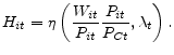
$\displaystyle H_{it}=\eta \left(\frac{W_{it}}{P_{it}}\frac{P_{it}}{P_{Ct}},\lambda_{t}\right).$

(2)

In this equation,

is the wage in industry

is the consumption goods price deflator, and $\lambda$ is the marginal utility of wealth. Labor supply depends positively on both arguments. The first argument is just the consumption wage, which we have written as the product wage in industry

times the relative price of industry

. Potentially, we could include a third term as well, consisting of the industry relative wage. For example, if the expanding industry must pay an overtime premium, as in one of the models analyzed by Ramey & Shapiro (1998) or if there are adjustment costs of labor across industries, as in Kline (2008), then it is possible that the wage in an expanding industry rises relative to wages in other industries.

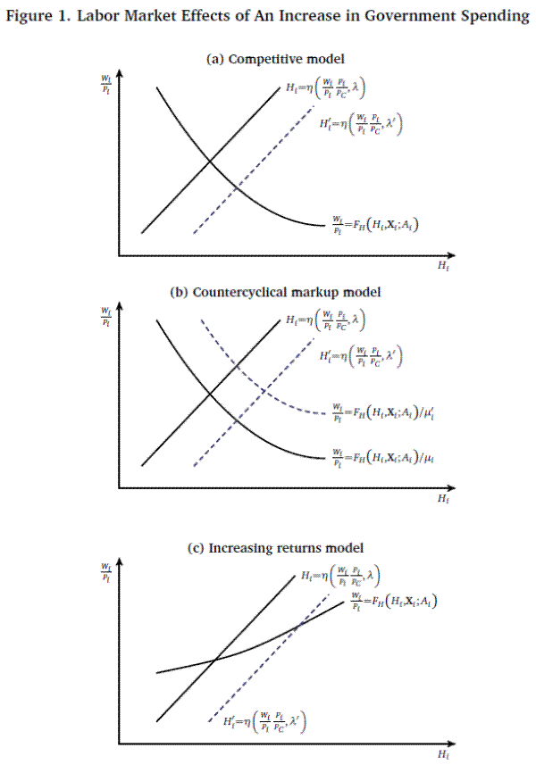
Figure 1 combines these supply and demand equations to show equilibrium in the industry's labor market. Panel (a) considers the labor market effects of an increase in government spending in the neoclassical model. The increase in government spending raises the marginal utility of wealth, which shifts the aggregate labor supply curve out. If the industry receives more of the government demand, then the industry price should rise relative to other prices. Thus, ${P_i}/{P_C}$ should rise, which also shifts out labor supply to this industry. As a result, equilibrium hours rise and the real product wage and productivity fall.

In contrast, an industry that does not receive any increase in government spending may experience a decline in ${P_i}/{P_C}$ that is large enough to counteract the rise in $\lambda$ . In this case, labor supply curve shifts in. Thus, this industry would experience a decline in hours, an increase in the real product wage and an increase in productivity.

Panel (b) considers the effects of countercyclical markups in the New Keynesian model for an industry receiving part of the increase in government spending. Because the negative wealth effect is still operative in the standard New Keynesian model, the supply curve shifts out, but now the demand curve also shifts out because the markup has fallen. The graph makes clear that the expansionary effect on equilibrium hours is even greater, but the effect on the real wage is ambiguous. Nevertheless, productivity still falls.

Panel (c) considers the increasing returns model of Devereux et al. (1996). In their model, firm-level labor demand curves slope down, but if returns to specialization are sufficiently high, industry-level demand curves can slope upward. In this case, the shift out of labor supply to the industry can lead to a rise in hours, real wages, and productivity.

To summarize, the neoclassical model predicts that an increase in government spending raises an industry's hours, but lowers its real wage and labor productivity. The standard New Keynesian model predicts an increase in hours, a decline in productivity, and an ambiguous effect on real wages. The increasing returns model predicts a rise in hours, real wages and productivity.

4 Data and Variable Construction

This section describes our data sources and explains how we construct the variables. Throughout the paper, uppercase letters represent real quantities and a tilde indicates a nominal quantity. Lowercase letters indicate the natural logarithm of a variable. The subscript denotes industry and denotes year. When possible, these subscripts are omitted in the text; however, they remain in all equations.

4.1 Industry-Specific Government Spending

Our sources for constructing industry-specific government spending are the benchmark IOccounts, which are available roughly quinquennially, in 1947, 1958, 1963, 1967, 1972, 1977, 1982, 1987, 1992, 1997 and 2002. The IOccounts for 1947 and 1958 do not contain the industry detail required, so we drop these observations. The last two IOccounts, 1997 and 2002, are based on the North American industrical classification system (NAICS) rather than the Standard Industrial Classification (SIC). Because merging the NAICSith the SICndustries is difficult and fraught with potential error, we also drop 1997 and 2002. Thus, we use information from the 1963, 1967, 1972, 1977, 1982, 1987, and 1992 IOccounts.

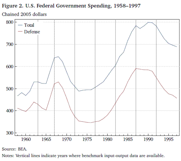
Figure 2 shows real federal spending and real defense spending from 1958 to 1997. The vertical lines indicate the years for which the IOccounts are available. The figure makes clear that almost all fluctuations in federal government purchases are due to defense spending. Defense spending started increasing in 1965 after Johnson sent bombing raids over North Vietnam in February 1965. Defense spending peaked in 1968 at the height of the Vietnam War, and then fell until the mid-1970s. It began to rise in 1979, and then accelerated starting in 1980 after the Soviet Union invaded Afghanistan in December 1979. Spending peaked in 1987, fell gradually until 1990, and then fell more steeply.

We use the IOccounts to compute the sum of direct and indirect government spending. This comprehensive measure captures downstream effects of an industry's spending. For example, an increase in government purchases of finished airplanes likely also increases shipments of aircraft parts industries that supply parts to the aircraft industries. Because it is difficult to distinguish nondefense from defense spending when calculating indirect effects, we use total federal government spending. As the previous figure shows, using all federal spending rather than just defense should not be problematic because most of the level and variation in federal government purchases is defense spending. Moreover, some spending not classified as defense, such as that for the National Aeronautics and Space Administration, is often driven by defense considerations.

To compute federal government demand, we use the "Transactions" and "Total Requirements" tables available from the IOccounts. Let $\tilde{S}^{\mathrm{IO}}_{ijt}$ be the nominal value of inputs produced by industry shipped to industry in year , measured in producers' prices. Nominal direct government demand, $\tilde{G}^{d}$ , for industry in year is the value of inputs from industry shipped to the federal government ():

$\displaystyle \tilde{G}^{d}_{it} = \tilde{S}^{\mathrm{IO}}_{igt}.$

(3)

Indirect government demand, $\tilde{G}^{n}$ , is calculated using commodity-by-commodity unit input requirement coefficients. Let $r_{ijt}$ be the commodity output required per dollar of each commodity delivered to final demand in year . The indirect government demand for industry 's output is the direct government purchases from industry times the unit input requirement of industry for industry 's output:

$\displaystyle \tilde{G}^{n}_{it} = \sum_{j=1}^{J_t} \tilde{G}^{d}_{jt} \times r_{ijt}.$

(4)

Total government demand for industry

in year

is the sum of direct and indirect demand:

$\displaystyle \tilde{G}_{it} = \tilde{G}^{d}_{it} + \tilde{G}^{n}_{it}.$

(5)

Perotti (2008) defined his government demand variable as the change in an industry's shipments to the government between two benchmark years divided by total initial shipments of the industry, i.e., $[G_{it} - G_{i(t-5)}]/S_{i(t-5)}$ . His measure is potentially problematic, though, because it makes the questionable assumption that the distribution of government spending across industries is uncorrelated with industry technological change. As we will argue below, we have reason to believe that his measure is correlated with industry-specific technological change.

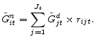
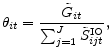
We therefore construct an alternative measure of a government demand shock that should not be correlated with industry-specific technology. In particular, we define the growth in government demand for industry , $\Delta g_{it}$ , as

$\displaystyle \Delta g_{it} = \theta_i \cdot \Delta g_{t},$

(6)

where $\theta_i$ is the average share of an industry's total nominal shipments that go to the government and $g_{t}$ is log of aggregate real federal spending (based on national income and product accounts (NIPA) data). We calculate the share of industry

's total nominal shipments that go to the government in year

$\displaystyle \theta_{it} = \frac{\tilde{G}_{it}}{\sum_{j=1}^{J} \tilde{S}^{\mathrm{IO}}_{ijt}},$

(7)

We then calculate industry

's average dependence on the government, $\theta_{i}$ , by averaging over all IOears (1963-92). Table 1 shows the 15 industries with the largest share of shipments to the government. Not surprisingly, most are defense industries.

Thus, our new measure converts the aggregate government demand variable into an industry specific variable using the industry's long-term dependence on the government as a weight. The idea behind this measure is that a given increase in aggregate government spending should have a bigger impact on an industry that, on average, sends a higher fraction of its output to the government. We could, in principle, use a time-varying weight using the individual IOables. We decided against this approach because of concern that changes in technology could drive changes in industry shares over time. On the other hand, if there is a correlation between industry long-run average technology growth and the long-run average industry government shipment share, it will be accounted for in the empirical analysis by industry fixed effects.

4.2 Variables from the Manufacturing Industry Database

The Manufacturing Industry Database (MID)Manufacturing Industry Database (MID) maintained by the NBERnd Center for Economic Studies (CES), contains annual data for 458 4-digit SICode manufacturing industries from 1958 to 1996.⁶Most of the information is derived from the Annual Survey of Manufacturers (ASM). We use the version based on the 1987 SICodes.⁷

The database provides information on hours only for production workers. We created two measures of total hours using two extreme assumptions: nonproduction workers always work 1,960 hours per year and nonproduction workers always work as much as production workers. This figure is slightly less than the usual 2000 hours per year because it allows for vacations and holidays, which are not included in production worker hours measures. The results were very similar, so we only report the results using the assumption that nonproduction workers always work 1,960 hours per year. The production worker product wage is the production worker wage bill divided by production worker hours times the shipments deflator.

For one set of results, we construct share-weighted growth of inputs. The payroll data from the MIDnclude only wages and salaries, and do not include payments for benefits, such as Social Security and health insurance. Thus, labor share estimates from this database are biased downward. Fortunately, Chang & Hong (2006) have compiled annual information for each 2-digit manufacturing industry from the NIPAf the ratio of total compensation to wages and salaries. We merge these factors to our 4-digit data and use them to magnify the payroll data to create more accurate labor shares.

We construct real shipments by dividing nominal shipments by the shipments price deflator. However, because firms hold inventories, shipments are not necessarily equal to output. According to the standard inventory identity, real gross output, , is equal to real shipments, , plus the change in real finished-goods and work-in-process inventories, $I^{F}$ . The MIDatabase reports only the total value of inventories, , at the end of the year; it does not distinguish inventories by stage of process in the reported stocks.

Fortunately, we can back out the nominal change in materials inventories from other data in the MID In particular, the measure of nominal value added, $\tilde{V}$ , in the MIDs defined as:

$\displaystyle \tilde{V}^{\mathrm{MID}}_{it} = \tilde{S}_{it} - \tilde{M}_{it} + \Delta \tilde{I}^{F}_{it},$

(8)

where $\tilde{M}$ is nominal materials cost.

Since total inventories is the sum of finished-goods and work-in-process inventories and materials inventories, $I^{M}$ , the change in materials inventories can be inferred from the change in total inventories and the change in finished-goods and work-in-process inventories: $\Delta \tilde{I}^{M}_{it} = \Delta \tilde{I}_{it} - \Delta \tilde{I}^{F}_{it}$ . Using this inventory relationship, we calculate real gross output as

$\displaystyle Y_{it} \approxeq \frac{\tilde{S}_{it}}{P_{it}} + \left[\frac{\tilde{I}_{it}}{P_{it}} - \frac{\tilde{I}_{i(t-1)}}{P_{i(t-1)}}\right] - \frac{\Delta \tilde{I}^{M}_{it}}{P_{it}},$

(9)

where

is the price of output. This formulation for gross output is not exact because the last term, the change in real materials inventories, should be

$\displaystyle \dfrac{\tilde{I}^{M}_{it}}{P_{it}} - \dfrac{\tilde{I}^{M}_{i(t-1)}}{P_{i(t-1)}}.$

Unfortunately the MIDoes not have data on the stock of materials inventories at each point in time necessary. As a result, our measure of gross real output in equation 9 understates production by

$\displaystyle \dfrac{\tilde{I}^{M}_{i(t-1)}}{P_{i(t-1)}} \times \dfrac{P_{it}-P_{i(t-1)}}{P_{it}},$

(10)

which is the product of the real initial stock of materials inventories (valued at output prices) and the rate of inflation of output prices. According to Bureau of Economic Analysis (BEA) estimates of inventories and sales in manufacturing, the real stock of materials inventories is about 50 percent of monthly sales, or about 4 percent of annual sales. Even if annual inflation is as high as 10 percent, the bias would only be -0.4 percent.

Many studies have used value added measures of output. However, Norrbin (1993) discusses the biases associated with using value added rather than gross output, and Basu & Fernald (1997) argue that value added is only valid with perfect competition and constant markups of unity. Thus, we do not use value added as a measure of output.

We also use MIDeasures of total capital, plant, equipment, investment, materials usage and energy usage. The MIDlso includes price indexes for capital, investment, materials, and energy. We create real series from the nominal values by dividing by the appropriate price index.

We merge the MIData with the IOata by developing a correspondence between the 6-digit IOode-based IOata and the 4-digit SICode-based MIData.⁸ The merged database contains 272 industries at the 4-digit SICevel. Because some of the industries were combined in the merge, we had to aggregate some variables from the MID The real quantities were defined at the industry level as the nominal quantities divided by the relevant price index. Because the price indices in this data base are fixed-weight indices, it is possible to sum the real quantities. We then summed nominal and real quantities for the combined industries and used their ratios to construct price indices.

5 Empirical Results

5.1 Properties of Industry-Specific Government Demand

The usefulness of our government demand variable for distinguishing between the various theories depends on two key features. First, in order for it to represent only shifts in industry demand, it must be uncorrelated with technology. Second, it should be relevant, in the sense that it is sufficiently correlated with industry output or hours. In this section, we assess how well the government demand variable satisfies these two properties.

At the aggregate level, there is substantial evidence that fluctuations in military spending are mostly driven by geopolitical events and are for the most part exogenous to the current state of the economy.⁹ Since most variations in federal purchases are due to military spending, it is unlikely that aggregate shipments to the government are correlated with technology. That said, it is possible that the distribution of military spending across industries could be related to technological change. To see why technology might influence government spending at the industry level, consider the following example. Between 1972 and 1977, real federal spending declined by 3 percent and real defense spending fell by 9 percent. In contrast, total real federal purchases of computers (SIC 3571) rose by 219 percent over this period. This increase was 20 percent of the initial value of shipments in 1972, yet the fraction of shipments that went to the government rose only slightly, from 7 percent in 1972 to 9 percent in 1977 because industry shipments to nongovernment destinations also rose dramatically. Clearly, the increase in government spending on computers during this period was not due to a "demand shift," but rather because technological change in the computer industry shifted government demand toward that industry and away from other industries. In other words, it is likely that the rise in industry-specific government spending was correlated with industry-specific technology growth.

It is for this reason that we do not adopt Perotti's definition of shifts in government demand. Perotti (2008) compared the change in shipments to the government over a five-year period to the initial total shipments of the industry. By his definition, the increase in computer shipments to the government would be classified as a very large demand shock, whereas it is clear that it was linked to industry-specific technological change.

The second desirable feature for our demand shifter is relevance. Is our government demand variable sufficiently correlated with output and hours? To investigate this feature, table 2 reports reduced-form regressions of the log change of two output measures and three labor measures on the government demand variable. The first row reports the results of a simple regression of the growth in real gross shipments on the growth of our government demand variable ( $\Delta g$ ). The coefficient is 1.84 (standard error of 0.16), implying that a 1-percent increase in aggregate federal spending causes shipments to rise by almost 1 percent in an industry that on average ships 50 percent of its output to the government. The coefficient is estimated very precisely. Although the is very low, the statistic on the coefficient is 128, implying that our government demand variable is very relevant. The second row estimates this specification including year and industry fixed effects. The estimate is higher, at 2.46 (0.17), and is highly significant. The third row of table 2 shows the fixed-effects regression of the growth in real gross output (which includes changes in work-in-process and finished goods inventories) on the growth of government demand. The estimated coefficient is 2.38 (0.18), statistically identical to that from the regression with shipments (line 2). In every case our government spending variable is highly relevant.

Rows 4-6 of table 2 report the estimated effects of changes in government demand on production worker hours and employment. All regressions include year and industry fixed effects. Row 4 shows the impact on production worker hours. The coefficient is 2.61 (0.16), which is somewhat above the coefficient for output. The government demand variable is also relevant for this variable, as evidenced by the implied statistic. Rows 5 and 6 show that virtually all of the change is due to changes in employment rather than average hours per worker.

To summarize the results of this section, the evidence shows that the new government demand variable we constructed is a very relevant instrument for shifts in output and hours. We have presented evidence that Perotti's measure may be correlated with industry-specific technology. In contrast, we have constructed our demand measure so that it is not subject to this problem.

5.2 Government Demand Effects on Prices and Productivity

5.2.1 Wages and Prices

Table 3 shows the results of instrumental variables (IV) regressions of wages and prices on total production worker hours. To isolate the effect of a government-demand induced rise in hours on wages and prices, we instrument for hours using our government demand variable. In particular, we regress the log change in product wages on the log change in hours, which is instrumented by the government demand variable. Row 1 shows that a government demand-induced increase in hours leads to a small decline in the relative real product wage. The estimate is statistically significant at the 7 percent level, but is economically small. Row 2 shows that an industry's relative wage does not change significantly, whereas row 3 shows that the relative price of an industry's rises.¹⁰ Thus, the decline in the real product wage is mostly due to a rise in the relative product price. These results are qualitatively consistent with the competitive model shown in section 3.

These results stand in contrast to Perotti's conclusion that government spending raises real wages. Perotti used similar data sources, but based his analysis on ranking the top industries receiving government spending from 1963 to 1967 and from 1977 through 1982. Based on visual inspection of his table, he concluded that "the sectors that experience the largest government spending shocks are also the sectors that experienced the largest positive changes in the real product wage.",¹¹

To determine the source of the differences in our conclusions, we construct Perotti's government demand instrument, which is available only as five-year differences due to the frequency of the IOables. We then regress the five-year log change in the real product wage on the five-year log change in hours, instrumented by this government demand variable. The coefficient is 0.15 (0.07), indicating a significant increase in real wages. However, when we include time and industry fixed effects in the regression, we obtain a coefficient of (0.06). Thus, Perotti's finding of a positive effect of government spending on real wages is due both to his definition of the government spending shock (with its potential correlation with technology) and his failure to account for industry and time fixed effects. When we use our annual government spending shock and include industry and time fixed effects, we find a small negative effect on real product wages.

5.2.2 Labor Productivity

We next investigate the effects of a government demand-induced rise in hours on labor productivity. To understand the interpretation of the coefficient, consider the special case of a Cobb-Douglas production function where the exponent on labor is $\alpha$ . The growth of labor productivity is given by

$\displaystyle \Delta (y _{it} - h^{\mathrm{p}}_{it}) = (\alpha - 1)\Delta h^{\mathrm{p}}_{it} + \beta \cdot \Delta x_{it} + \Delta a_{it},$

(11)

where

is the log of real output, $h^\mathrm{p}$ is the log of production-worker hours,

is the share-weighted log of other inputs, and

is the log of technology. If there is no change in other inputs, then our government demand instrument is valid for estimating $\alpha - 1$ since the instrument is uncorrelated with technology

. On the other hand, if other inputs are also increasing, then the demand instrument will be positively correlated with the error term and the estimate of $\alpha - 1$ will be biased upward.

Rows 4 and 5 of table 3 shows the effect of a government demand-induced rise in hours on two measures of the growth in labor productivity. In each case, we divide an output measure by total hours of production workers. Both equations include year and industry fixed effects. The first measure uses real gross shipments and the second uses real gross output (equation 9). In both cases, the coefficient is small but negative, implying that a rise in hours leads to a slight decline in labor productivity. If we believe that other inputs are fixed, then the coefficient implies a high value of $\alpha$ of 0.91 or 0.94. As we will show below, however, other inputs do rise in response to government spending shock. Thus, this estimate is likely an upper bound on $\alpha$ .

5.2.3 Markup

We can combine the results for productivity and real wages to determine the implications for the countercyclical markup hypothesis that is key to the New Keynesian explanation of fiscal policy. To see this, consider the definition of the log change in the markup:

$\displaystyle \Delta \mu _{it} = \Delta \left(y_{it} - h^{\mathrm{p}}_{it}\right) - \Delta \left(w_{it} - p_{it}\right),$

(12)

where

is the log of the nominal wage and

is the log of the output price.

Rows 6 and 7 of table 3 show IVegressions of the change in the markup on the change in total production worker hours. We calculate the markup with two output measures, one using real shipments and the other using real gross output. Both measures of the markup are essentially constant in response to an increase in hours. In one case, the coefficient estimate is 0.02 (0.05) and in the other it is -0.01 (0.04), but in neither case is it statistically different from zero. Thus, markups appear to be constant in response to a shift in government demand.

5.3 Effects of Government Demand on Other Inputs

We now investigate the effects of government spending on several other key inputs. We begin by studying the responses of particular inputs. We then construct a share-weighted measure of inputs and estimate the implied returns to scale.

5.3.1 Other Inputs

Table 4 reports the reduced-form response of various inputs to industry-specific government spending changes. The first row reproduces the response of production worker hours for comparison. Supervisory worker employment increases significantly (row 2), but the response, 2.33 (0.19), is smaller than for production workers hours (row 1), 2.61 (0.16). Thus, the ratio of supervisory workers to production workers declines when government demand increases.

Rows 3-5 investigate the response of various measures of capital inputs. Row 3 shows the response of the real capital stock. The response is positive and significant, but with a coefficient of 0.50 (0.06) it is much smaller than for labor. Thus, the increase in government spending leads to a decline in the capital-labor ratio. It is possible, however, that capital services could rise by more than the capital stock if capital utilization increases in response to government spending. To investigate this possibility, we consider two measures of capital utilization that have been used in the literature. The first measure is energy usage. Numerous papers have used electricity consumption as an indirect measure of capital utilization.¹² We do not have information in our data set on electricity consumption, but we do have information on overall energy usage. Thus, the fourth row of table 4 reports the response of real energy usage. The coefficient estimate is 0.42 (0.21). If utilization is proportional to energy usage, then we can combine this estimate with the growth of capital of 0.50, to infer that capital services rise by 0.92. While larger than the basic estimate, it is still far below the rise in production worker hours. The second indicator of capital utilization we consider is Shapiro's measure of the workweek of capital, which is based on the Census Bureau's Survey of Plant Capacity. This measure counts hours per day and days per week that a plant operates. Shapiro (1993) used this measure to show that the Solow residual is no longer procyclical once this utilization measure is included. Unfortunately, Shapiro's measure is only available from 1977 to 1987 and only for a subset of the industries. Row 5 reports the effects of government spending on this measure. The coefficient is -0.61 (0.79) and is not statistically significant. Thus, this alternative source does not raise the estimate of the growth of capital services.

Row 6 shows the response of real materials inputs excluding energy. In this case, the response is 2.70 (0.20), slightly larger than for hours or output. Row 7 shows the results for the ratio of real materials to output. The coefficient is 0.32 (0.13) and is statistically significant from zero.

5.3.2 Implications for Returns to Scale

To study the response of other inputs more systematically, we can estimate the overall returns to scale using the framework pioneered by Hall (1990), and extended by Basu & Fernald (1997). In particular, we can estimate overall returns to scale from the following equation:

$\displaystyle \Delta y_{it} = \gamma \Delta z_{it} + \Delta a_{it},$

(13)

where $\Delta z$ is the share-weighted growth of all inputs. The coefficient $\gamma$ measures the returns to scale. If technology is the only source of error in this equation, then one can estimate $\gamma$ by using a demand instrument that is correlated with input growth but uncorrelated with technology.

Consider a measure of share-weighted input growth treating energy as an input to production:

$\displaystyle \Delta z_{it} = s_{k} \Delta k_{it} + s_{h}\Delta h_{it} + s_{m}\Delta m_{it} + s_{e}\Delta e_{it},$

(14)

where

is the log of the real capital stock,

is the log of total hours,

is the log of real materials usage,

is the log of real energy usage, and $s_{j}$ is the share of input

. As discussed in section 4.2, we construct the labor share (

) using Chang & Hong's factors to inflate the observed labor share to account for fringe benefits. This raises the average labor share in the data set by 3 percentage points. Following Basu et al. (2006), we calculate the capital share as the residual from labor share and materials share and by using shares averaged over the entire sample.

We estimate the return to scale using an IVegression of the growth of log gross output on the share-weighted growth of inputs and on year and industry fixed effects. We instrument for $\Delta z$ with our government demand variable ( $\Delta g$ ). The first-stage regression of the share-weighted inputs on our government variable has an statistic that exceeds 200, indicating high relevance. The first row of table 5 reports the IVegression. The estimated coefficient is 1.11 (0.05), indicating small, marginally statistically-significant increasing returns to scale.

However, as numerous papers have made clear, unobserved variations in capital utilization or labor effort may contaminate the error term.¹³ Because these variations are likely to be correlated with any instrument that is also correlated with observed input growth, estimates of $\gamma$ are likely to be biased upward. We attempt to mitigate this bias in two ways. The first is to include a proxy for unobserved utilization. The second is to construct $\Delta z$ treating energy usage as a proxy for capital utilization.

Basu et al. (2006) use the theory of the firm to show that, under certain conditions, unobserved variations in capital utilization and labor effort are proportional to the growth in average hours per worker. Row 2 of table 5 adds the growth of average hours per worker ( $\Delta \bar{h}$ ) to control for unobserved utilization. The estimate of the return to scale is little changed. Nevertheless, this specification is probably invalid because $\bar{h}$ is uncorrelated with technology only under restrictive assumptions.

Although $\Delta g$ is highly relevant for $\Delta z$ , it is difficult to find additional relevant instruments for $\Delta \bar{h}$ . We attempt to create extra instruments by using separate measures of direct and indirect government shipments and a quadratic in total government shipments as instruments for both variables. All statistics (such as Shea's partial ) suggest the instruments have low relevance for $\Delta \bar{h}$ after being used for $\Delta z$ .¹⁴ Row 3 of table 5 reports the results of this IVegression. The estimate of the return to scale is little changed at 1.09 (0.06) and the coefficient on average hours per worker is not significantly different from zero. Nonetheless, we are not very confident of this specification given the weak instruments.

A second approach to mitigate unobserved utilization is to construct $\Delta z$ treating capital utilization as proportional to energy usage. This alternate measure of share-weighted input growth is

$\displaystyle \Delta z_{it} = s_{ke}\left(\Delta k_{it} + \Delta e_{it}\right) + s_{h}\Delta h_{it} + s_{m^{\mathrm{x}e}}\Delta m^{\mathrm{x}e}_{it},$

(15)

where $m^{\mathrm{x}e}$ is the log of real materials usage excluding energy. As before, we instrument for $\Delta z$ with $\Delta g$ . Row 4 of table 5 reports the regression using this alternate measure of input growth. The estimated coefficient, 1.07 (0.05), is not statistically different from unity, implying constant returns to scale.

In sum, our results are completely consistent with the neoclassical assumptions concerning the effects of government spending. An increase in output induced by government spending raises hours, but lowers real wages and productivity. Taking all inputs into account, we cannot reject constant returns to scale.

6 Conclusion

Our study of the effects of industry-specific changes in government spending indicates that an increase in government demand raises an industry's relative output and hours. These increases are associated with small declines in its relative real wage and labor productivity, and a rise in its relative price. Its use of other inputs, such as capital, energy, and materials, rises as well. Our estimates of returns to scale are consistent with constant returns to scale. Thus, the results support the microeconomic assumptions underlying the neoclassical theory of the effects of government spending. In contrast, we find no evidence of the rising real wages or countercyclical markups that are central to the standard New Keynesian explanation for the effects of government spending.

A key question, then, is why aggregate evidence indicates that an increase in government spending raises labor productivity whereas the industry-level evidence presented in this paper indicates that an increase in demand associated with higher government spending lowers labor productivity slightly. Basu & Fernald (1997) provide an answer based on their extensive study of the effects of aggregation on returns to scale estimates. They show that durable goods manufacturers have higher returns to scale than many other industries, some of which exhibit sharply diminishing returns to scale. Thus, anything that shifts output toward durable goods producers will lead to aggregate behavior that looks like increasing returns to scale. The 15 industries that depend most on government spending are all durable goods manufacturing industries. Thus, the increase in aggregate labor productivity in response to government spending can be explained by reallocation rather than by firm-level or industry-level increasing returns.

References

Bibliography

E. J. Bartelsman, et al. (2000).

`NBER-CES Manufacturing Industry Database'.
Tech. rep., National Bureal of Economic Research.

M. J. Barth & V. A. Ramey (2002).

`The Cost Channel of Monetary Transmission'.
In B. S. Bernanke & J. Rotemberg (eds.), NBER Macroeconomics Annual 2001, pp. 199-256. University of Chicago Press.

S. Basu (1996).

`Procyclical Productivity: Increasing Returns or Cyclical Utilization?'.
The Quarterly Journal of Economics 111(3):719-51.

S. Basu & J. G. Fernald (1997).

`Returns to Scale in US Production: Estimates and Implications'.
Journal of Political Economy 105(2):249-83.

S. Basu, et al. (2006).

`Are Technology Improvements Contractionary?'.
American Economic Review 96(5):1418-48.

M. Baxter & R. G. King (1993).

`Fiscal Policy in General Equilibrium'.
American Economic Review 83(3):315-34.

C. Burnside, et al. (2004).

`Fiscal Shocks and Their Consequences'.
Journal of Economic Theory 115(1):89-117.

C. Burnside, et al. (1996).

`Capital Utilization and Returns to Scale'.
In B. S. Bernanke & J. J. Rotemberg (eds.), NBER Macroeconomics Annual 1995, pp. 67-124. National Bureau of Economic Research.

M. P. Cavallo (2005).

`Government Employment and the Dynamic Effects of Fiscal Policy Shocks'.
Working Papers in Applied Economic Theory 2005-16, Federal Reserve Bank of San Francisco.

Y. Chang & J. H. Hong (2006).

`Do Technological Improvements in the Manufacturing Sector Raise or Lower Employment?'.
American Economic Review 96(1):352-68.

M. B. Devereux, et al. (1996).

`Monopolistic Competition, Increasing Returns, and the Effects of Government Spending'.
Journal of Money, Credit & Banking 28(2):233-54.

A. Fatás & I. Mihov (2001).

`The Effects of Fiscal Policy on Consumption and Employment: Theory and Evidence'.
Unpublished paper, INSEAD and CEPR.

J. Galí, et al. (2007).

`Understanding the Effects of Government Spending on Consumption'.
Journal of the European Economic Association 5(1):227-70.

R. E. Hall (1990).

`Invariance Properties of Solow's Productivity Residual'.
In P. Diamond (ed.), Growth, Productivity, Employment. MIT Press.

D. W. Jorgenson & Z. Griliches (1967).

`The Explanation of Productivity Change'.
The Review of Economic Studies 34(3):249-83.

P. Kline (2008).

`Understanding Sectoral Labor Market Dynamics: An Equilibrium Analysis of the Oil and Gas Field Services Industry'.
Discussion paper 1645, Cowles Foundation, Yale University.

S. C. Norrbin (1993).

`The Relation between Price and Marginal Cost in U.S. Industry: A Contradiction'.
Journal of Political Economy 101(6):1149-64.

M. Ouyang (2009).

`On the Cyclicality of R and D'.
Working paper, UC Irvine.

E. Pappa (2005).

`New Keynesian or RBC Transmission? The Effects of Fiscal Policy in Labor Markets'.
Working Paper 293, Innocenzo Gasparini Institute for Economic Research, Bocconi University.

R. Perotti (2004).

`Estimating the Effects of Fiscal Policy in OECD Countries'.
Working Paper 276, Innocenzo Gasparini Institute for Economic Research, Bocconi University.

R. Perotti (2008).

`In Search of the Transmission Mechanism of Fiscal Policy'.
In D. Acemoglu, K. Rogoff, & M. Woodford (eds.), NBER Macroeconomics Annual 2007, pp. 169-226. University of Chicago Press.

V. A. Ramey (2008).

`Comment on `In Search of the Transmission Mechanism of Fiscal Policy".
In D. Acemoglu, K. Rogoff, & M. Woodford (eds.), NBER Macroeconomics Annual 2007, pp. 169-226. University of Chicago Press.

V. A. Ramey (2009a).

`Defense News Shocks, 1939-2008: Estimates Based on News Sources'.
Unpublished paper, University of California, San Diego.

V. A. Ramey (2009b).

`Identifying Government Spending Shocks: It's All in the Timing'.
Working paper 15464, National Bureau of Economic Research.

V. A. Ramey & M. D. Shapiro (1998).

`Costly Capital Reallocation and the Effects of Government Spending'.
Carnegie-Rochester Conference Series on Public Policy 48:145-94.

J. J. Rotemberg & M. Woodford (1991).

`Markups and the Business Cycle'.
In O. J. Blanchard & S. Fischer (eds.), NBER Macroeconomics Annual 1991, pp. 63-129. MIT Press.

J. J. Rotemberg & M. Woodford (1992).

`Oligopolistic Pricing and the Effects of Aggregate Demand on Economic Activity'.
Journal of Political Economy 100(6):1153-207.

M. D. Shapiro (1993).

`Cyclical Productivity and the Workweek of Capital'.
American Economic Review 83(2):229-33.

J. Shea (1993).

`Do Supply Curves Slope up?'.
Quarterly Journal of Economics 108(1):1-32.

J. Shea (1997).

`Instrument Relevance in Multivariate Linear Models: A Simple Measure'.
Review of Economics and Statistics 79(2):348-52.

Table 1: Industries with Largest Share of Shipments to the Government
Rank	SIC	Industry	$\theta_i$
1	3761	Guided missiles and space vehicles	0.920
2	3483	Ammunition, except for small arms, n.e.c.	0.807
3	3489	Ordnance and accessories, n.e.c.	0.769
4	3728	Aircraft and missile equipment, n.e.c.	0.628
5	3731	Ship building and repairing	0.626
6	3724	Aircraft and missile engines and engine parts	0.610
7	3663	Communication equipment	0.496
8	3721	Aircraft	0.491
9	3795	Sighting and fire control equip.	0.489
10	3812	Engineering and scientific instruments	0.435
11	3463	Nonferrous forgings	0.419
12	3482	Small arms ammunition	0.384
13	3339	Primary nonferrous metals, n.e.c.	0.321
14	3672	Other electronic components	0.294
15	3674	Semiconductors and related devices	0.282

Source: Author's calculations using data from BEA benchmark IO tables.

Notes: $\theta_i$ is the average share of industry 's total nominal shipments that go to the federal government. Calculated from a panel of 274 industries in 1963, 1967, 1972, 1977, 1982, 1987, and 1992.

Table 2: Reduced-Form Regressions of Industry Output and Labor on Government Demand
Dependent variable	Independent variable $\Delta g_{it}$	Fixed effects	Partial
Output measure 1. Real shipments	1.836 ^***	No	0.013
Output measure 1. Real shipments (standard error)	(0.162)
Output measure 2. Real shipments	2.464 ^***	Yes	0.020
Output measure 2. Real shipments (standard error)	(0.172)
Output measure 3. Real gross output	2.376 ^***	Yes	0.017
Output measure 3. Real gross output (standard error)	(0.182)
Production worker measure 4. Total hours	2.610 ^***	Yes	0.027
Production worker measure 4. Total hours (standard error)	(0.155)
Production worker measure 5. Employment	2.572 ^***	Yes	0.029
Production worker measure 5. Employment (standard error)	(0.149)
Production worker measure 6. Average hours	0.038 ^***	Yes	0.000
Production worker measure 6. Average hours (standard error)	(0.056)

Source: Authors' regressions using data from the NBER-CES MID and BEA IO tables.

Notes: Dependent variable is annual change in the log of the output or labor variable listed. All labor variables refer to production workers. $\Delta g_{it}$ is the industry-specific change in government demand (see equation 6). All regressions have 10,135 observations from a panel of 274 industries over 1960-96; regressions include year and industry fixed effects when indicated. Standard errors are reported in parentheses. *** indicates significance at 1-percent, ** at 5-percent, and * at 10-percent level.

Table 3: Instrumental-Variables Regressions of Wages, Prices, Labor Productivity and Markups on Total Production Worker Hours
Dependent variable	Independent variable $\Delta h^{\mathrm{p}}_{it}$
Wages and prices: 1. Real wage	-0.076 ^*	0.170
Wages and prices: 1. Real wage (standard error)	(0.042)
Wages and prices: 2. Nominal wage	-0.015	0.299
Wages and prices: 2. Nominal wage (standard error)	(0.026)
Wages and prices: 3. Price of output	0.061 ^*	0.335
Wages and prices: 3. Price of output (standard error)	(0.034)
Productivity: 4. Measured with real shipments	-0.056	0.120
Productivity: 4. Measured with real shipments (standard error)	(0.047)
Productivity: 5. Measured with real gross output	-0.090 ^**	0.119
Productivity: 5. Measured with real gross output (standard error)	(0.049)
Markup: 6. Measured with real shipments	0.020	0.055
Markup: 6. Measured with real shipments (standard error)	(0.045)
Markup: 7. Measured with real gross output	-0.014	0.064
Markup: 7. Measured with real gross output (standard error)	(0.044)

Source: Authors' regressions using data from the NBER-CES MID and BEA IO tables.

Notes: Dependent variable is annual change of the log of the variable listed. Independent variable is the annual change of the log of total production worker hours ( $\Delta h^p_{it}$ ), instrumented by the industry-specific change in government demand ( $\Delta g_{it}$ , see equation 6). All regressions have 10,133 observations from a panel of 274 industries over 1960-96 and include year and industry fixed effects. Standard errors are reported in parentheses. *** indicates significance at 1-percent, ** at 5-percent, and * at 10-percent level.

Table 4: Reduced-Form Regressions of Other Inputs on Government Demand
Dependent variable	Independent variable $\Delta g_{it}$	Partial
1. Production worker total hours	2.610 ^***	0.027
1. Production worker total hours (standard error)	(0.155)
2. Supervisory worker employment	2.327 ^***	0.014
2. Supervisory worker employment (standard error)	(0.194)
3. Real capital stock	0.497 ^***	0.007
3. Real capital stock (standard error)	(0.060)
4. Real energy	0.419 ^**	0.001
4. Real energy (standard error)	(0.205)
5. Workweek of capital	-0.611	0.000
5. Workweek of capital (standard error)	(0.789)
6. Real materials excluding energy	2.700 ^***	0.017
6. Real materials excluding energy (standard error)	(0.204)
7. Real materials-output ratio	0.324 ^**	0.001
7. Real materials-output ratio (standard error)	(0.128)

Source: Authors' regressions using data from the NBER-CES MID and BEA IO tables.

Notes: Dependent variable is annual change in the log of the output or labor variable listed. All labor variables refer to production workers. $\Delta g_{it}$ is the industry-specific change in government demand (see equation 6). Regressions have 10,135 observations from a panel of 274 industries over 1960-96; regression with workweek of capital (row 5) has only 1,793 observations. All regressions include year and industry fixed effects. Standard errors are reported in parentheses. *** indicates significance at 1-percent, ** at 5-percent, and * at 10-percent level.

Table 5: Instrumental-Variables Regressions of Output Growth on Input Growth
Input growth definition	Independent variable $\Delta z_{it}$	Independent variable $\Delta \bar{h}_{it}$
1. Energy as input	1.108 ^***		0.743
1. Energy as input (standard error)	(0.049)
2. $\bar{h}$ as proxy for utilization, not instrumented	1.109 ^***	-0.013	0.743
2. $\bar{h}$ as proxy for utilization, not instrumented (standard error)	(0.049)	(0.025)
3. $\bar{h}$ as proxy for utilization, instrumented^a	1.093 ^***	0.856	0.688
3. $\bar{h}$ as proxy for utilization, instrumented^a (standard error)	(0.066)	(2.135)
4. Energy as proxy for utilization	1.065 ^***		0.692
4. Energy as proxy for utilization (standard error)	(0.051)

Source: Authors' regressions using data from the NBER-CES MID and BEA IO tables.

Notes: Dependent variable is annual change of log real output. $\Delta z_{it}$ is annual growth of share-weighted log inputs (including production worker hours); see equations 14 and 15. $\Delta \bar{h}_{it}$ is annual growth of average hours per worker. Except for row 3, $\Delta z_{it}$ instrumented by industry-specific change in government demand ( $\Delta g_{it}$ , see equation 6). All regressions have 10,133 observations from a panel of 274 industries over 1960-96 and include year and industry fixed effects. Standard errors are reported in parentheses. *** indicates significance at 1-percent, ** at 5-percent, and * at 10-percent level.

a. Both $\Delta z_{it}$ and $\Delta \bar{h}_{it}$ instrumented by direct shipments to government ( $\Delta g^d_{it}$ ), indirect shipments to government ( $\Delta g^n_{it}$ ), and the square of total shipments to government.

Figure 1: Labor Market Effects of An Increase in Government Spending. All three panels plot hours worked in industry $i$ ($H_i$) on the horizontal axis against the real wage ($W_i/P_i$) on the vertical axis. (a): Initial equilibrium is the intersection of a downward-sloping labor demand schedule (convex) and an upward-sloping labor supply schedule (linear). An increase in government spending raises the marginal utility of wealth, shifting out the labor supply schedule. The new intersection lies below and to the right of the initial equilibrium. (b): Initial equilibrium is as in panel (a). An increase in government spending raises the marginal utility of wealth, shifting out the labor supply schedule; the increase also reduces the markup, shifting out the labor demand schedule. The new intersection lies to the right of the initial equilibrium at roughly the same level of the real wage. (c): Initial equilibrium is the intersection of an upward-sloping labor demand schedule (convex) and an upward-sloping labor supply schedule (linear). An increase in government spending raises the marginal utility of wealth, shifting out the labor supply schedule. The new intersection lies above and to the right of the initial equilibrium.

Figure 2: U.S. Federal Government Spending, 1958-1997. Refer to link below for data

Figure 2 Data

Footnotes

1. See, for example, Baxter & King (1993). Return to Text

2. See, for example, Rotemberg & Woodford (1992). Return to Text

3. See, for example, Devereux et al. (1996). Return to Text

4. See, for example, Fatás & Mihov (2001), Perotti (2004), Pappa (2005), and Galí et al. (2007). Return to Text

5. See, for example, Burnside et al. (2004), Cavallo (2005), and Ramey (2009b). Return to Text

6. Bartelsman et al. (2000). Return to Text

7. Throughout the paper, all SICodes reported are the 1987 version. Return to Text

8. The correspondence tables are available on the authors' web sites. Return to Text

9. For example, Ramey (2009a). Return to Text

10. These results pertain to relative wages and prices because we have included time fixed effects. Return to Text

11. Perotti (2008), p. 208. Return to Text

12. See, for example, Jorgenson & Griliches (1967) and Burnside et al. (1996). Return to Text

13. See, for example, Burnside et al. (1996) and Basu (1996). Return to Text

14. Shea (1997). Return to Text

^♣ This version is optimized for use by screen readers. Descriptions for all mathematical expressions are provided in LaTex format. A printable pdf version is available. Return to Text