Skip to: [Printable Version (PDF)] [Bibliography] [Footnotes]

Finance and Economics Discussion Series: 2010-53 Screen Reader version ^♣

Mortgage Contract Choice in Subprime Mortgage Markets

Gregory Elliehausen

Federal Reserve Board and George Washington University

Min Hwang

George Washington University

May 20, 2010

Keywords: Mortgages, household financial decisions

Abstract:

The boom in the subprime mortgage market yielded many loans with high LTV ratios. From a large proprietary database on subprime mortgages, we find that choice of mortgage rate type is not linear in loan sizes. A fixed rate mortgage contract is a popular choice when loan size, measured by LTV ratio, is small. As LTV ratio increases, borrowers become more likely to choose adjustable rate mortgage contracts. However, when LTV reaches a certain level, borrowers start to switch back to fixed rate contracts. For these high LTV loans, fixed rate mortgages dominate borrowers' choices. We present a very simple model that explains this "nonlinear" pattern in mortgage instrument choice. The model shows that the choice of mortgage rate type depends on two opposing effects: a "term structure" effect and an "interest rate volatility" effect. When the loan size is small, the term structure effect dominates: rising LTV ratios making ARM loans less costly, and more attractive. However, when the loan size is large enough, the interest volatility effect dominates: rising LTV ratios making FRM loans less costly and preferable. We present strong empirical evidence in support of the model predictions.

JEL codes: G21, D10

1. Introduction

Adjustable-rate mortgage (ARM) products have long been an integral component of US mortgage markets, but their prevalence has varied substantially over time. ARM loans have existed since early 1970s and become very prevalent in early 1980s, when long-term Treasury rates exceeded 10 percent. By the mid-1980s, about two-thirds of mortgage loan originations were ARM loans¹. The share of ARM loans fell dramatically afterwards as long-term interest rates fell and remained relatively low until the early 2000s. The boom in housing prices, coupled with innovations in mortgage products in subprime market during the 2000s, stimulated renewed interest in ARMs.

The growth in the subprime mortgage market and the popularity of hybrid ARMs in that market contributed to the increased share of ARM lending in the 2000s. As is well known, subprime loans expose lenders to credit risk: They include loans to borrowers with impaired credit histories and loans with high loan-to-value (LTV) ratios, both of which are associated with higher probabilities of default. ARM loans were considered riskier than fixed-rate mortgage (FRM) loans, even in the prime market,² and the subprime market compounds these risks.

The subprime market provides a unique opportunity to examine choices of mortgage rate type over a wide range of risk characteristics. Figure 1 presents an interesting pattern of mortgage rate choice in the subprime market. It shows that the share of ARM loans among first lien mortgages increases steadily as the LTV ratio rises, but only up to about 90 percent LTV. Once past 90 percent, the share of ARM loans falls dramatically. At very high LTVs of 120 percent or higher, the share of ARM loans falls to 10 percent of the loans. In other words, the share of ARM loans in the subprime market is not monotonic in loan to value: It increases when loan size is relatively small but decreases when LTVs are relatively high. Figure 2 presents another piece of evidence suggesting that higher leverage may influence choice between FRM and ARM loans. Most additions to mortgage debt in through second mortgages involve fixed-rate loans. Indeed except for 2002, FRM loans account for more than 70 percent of second mortgages between 1998 and the first quarter of 2006.³ A large literature examines the choice of interest rate type for mortgages, but as far as we can establish, no study yet provides an explanation for this humped pattern of mortgage choices.

This paper uses a simple, two-period model to predict type of mortgage interest rate and then uses data on subprime mortgage originations to test predictions of the model. In the stylized model, risk neutral lenders offer both ARM and FRM contracts in a competitive market to risk neutral borrowers who ruthlessly exercise default options when they find default beneficial. The first period loan payment is assumed to determine borrowers' mortgage choices. Two factors drive the difference in the first period payments between two mortgage products: the slope of the yield curve (term spread) and interest rate volatility. With positive and large term spreads, rising LTV ratios raise FRM loan rates more than ARM margins, ("term structure effects"), rendering FRM loans more expensive for borrowers. With high interest rate volatility, rising LTV ratios raise ARM margins but have no effect on FRM rates. Higher interest rate volatility affects ARM margins through positive "payment shocks," which increase monthly payment size and enhance default probability of ARM loans. In a world where borrowers can default without recourse, lenders need to increase the margin on an ARM contract, rendering ARM loans more costly compared to FRM loans.

One can think of the interest rate volatility effect as augmenting the default option on ARMs. For FRM contracts, a default option depends only on the probability of the house value falling below the current loan balance. But for ARM contracts, the default option depends also on interest rate fluctuations. Recognizing the augmented option, lender will raise the margin for compensation. Moreover, this option depends on the loan size. As loan size increases, the option value increases, and so does the margin. At first, as LTV ratio rises, the "term structure effects" dominate, making ARM loans more attractive than FRM loans. However, beyond some value of LTV, the "interest rate volatility effect" causes the ARM margin to rise, making a FRM less costly and therefore preferable to an ARM.

The literature on the choice of mortgage contract is large and goes back for at least two decades (see Dhillon, Shilling and Sirmans 1987, Brueckner and Follain 1988, Tucker 1991, Goldberg and Heuson 1992 and Sa-Aadu and Sirmans 1995, for example). More recently, Posey and Yavas (2001) present a model with asymmetric information where borrowers' mortgage instrument choice serves as signal of default risks: high risk borrowers choose ARM loans while low-risk borrowers choose FRM loans in a separating equilibrium. Campbell and Cocco (2003) solve a dynamic life-cycle model of the optimal consumption and mortgage choice. They show that borrowers with FRM loans are exposed to wealth risks, while borrowers with ARM loans are exposed to income risks. Risks faced by ARM borrowers would be especially large in periods with relatively high interest rates combined with relatively low borrower income. Households with smaller houses (relative to income), more stable income, lower risk aversion and higher mobility would benefit from ARM loans. Campbell and Cocco further examine an inflation-indexed FRM loan that can potentially protect borrowers from wealth risks of existing FRM loans and income risks of ARM loans at the same time. Most recently, Koijen, van Hemert and van Nieuwerburgh (2009) propose the long-term bond risk premium as the main determinant for mortgage instrument choice, showing that a higher long-term bond risk premium is closely associated with a greater share of ARM loans. In their model, a FRM rate is tied to long-term bond yield, whereas an ARM rate depends on future short-term interest rates. They argue that financially unsophisticated borrowers are more likely to form adaptive expectations and use a simple average of past short-term interest rates as their expectation on future interest rates. They measure the difference in costs between a FRM mortgage and an ARM mortgage (that is, the long-term risk premium) as the five-year Treasury yield less a simple average of one-year Treasury yields. This paper contributes to the literature by examining more closely the interaction of the term structure and payment shock effects.

The rest of the paper is organized as follows. In section 2, we introduce the model and discuss its implications. Section 3 provides data description used in the empirical work. Section 4 provides empirical results. Section 5 concludes.

2. The Model

Consider a competitive mortgage market where risk neutral lenders offer to risk neutral borrowers adjustable rate mortgage contracts (ARM) and fixed rate mortgage contracts (FRM). Both mortgage contracts are interest-only and non-recourse. Lenders are assumed to rely on short-term borrowings from the capital market themselves to fund loans. We assume that lenders do not default.

2.1 Timeline of cash flows

We consider loan contracts over two periods. At the beginning of the first period, per request from a borrower, a lender obtains funds from the capital market at the current market interest rate and disburses them to the borrower. The borrower uses the loan to purchase home or refinance an existing mortgage. In case of an ARM contract, the mortgage rate for the first period is the market interest rate (index rate) of the first period plus the ARM margin. Therefore, at the time of contract, there is no uncertainty in ARM rate in the first period. At the end of the first period, the borrower makes the first payment to the lender, who, in turn, pays off its loan and borrows again to fund the second period. For simplicity, the loans are assumed to be interest-only, and the first period payment is the interest payment for the period. We assume that the lender does a thorough underwriting so that there is no possibility that borrower defaults on the payment in the first period. At the end of the second period, the borrower liquidates the house and closes the loan. If the house is sold at a price larger than the promised payment of interest payment and principal, the borrower will pay off the loan. If not, the borrower defaults, and the lender forecloses the house. The proceeds from the foreclosure are the selling price of the house. We assume that, even if the borrower defaults, the lender pays off the funds it borrowed from the capital market.

2.2 Lender's problem.

The lender offers two types of mortgage contracts, adjustable-rate contracts and fixed-rate contracts. To make a loan, the lender relies on the short-term financing from the capital market (warehousing): Either it borrows or renews the loan every period at the prevalent market interest rate.

If the lender makes a loan to a borrower on a fixed rate basis, then the lender's profit is

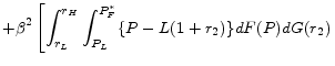
$\displaystyle \Pi_{F} = \beta(-Lr_{1}$		$\displaystyle +Li)$
		$\displaystyle +\beta^{2}\left[ \int_{r_{L}}^{r_{H}}\int_{P_{L}}^{P_{F}^{*}} \{ P-L(1+r_{2}) \} dF(P)dG(r_2) \right.$
		$\displaystyle \left. +\int_{r_{L}}^{r_{H}}\int_{P_{F}^{*}}^{P_{L}} \{ L(1+i) -L(1+r_{2})\} dF(P)dG(r_{2}) \right]$

where $r_{1}$ is the interest rate in the first period, $r_{2}$ , the interest rate in the second period, , the mortgage rate in the fixed rate contract, $\beta$ , the time discount factor for the lender, , a random value of the house at the end of the second period, and , the initial loan amount. Also $P_{F}^{*}$ is the level of house price at which the borrower chooses to default. We assume that there are no default costs, and borrowers ruthlessly default. Under these assumptions, $P_{F}^{*}$ is equal to , the payoff amount of the loan in the second period. The value of the house and the interest rate in the second period are random, uncorrelated and uniformly distributed over $[P_{L},P_{H}]$ and $[r_{L}, r_{H}]$ .

At the beginning of the first period, the lender borrows from the capital market, and lends it to the borrower so that there is no net cash flow for the lender. At the end of the first period, the lender receives a mortgage interest payment, , from the borrower, and pays the interest payment for its borrowing in the capital market, $Lr_{1}$ . The first period profit (cash flow) for the lender is $-Lr_{1}+Li$ . At the end of the second period, the borrower either pays off the loan or defaults on the loan. If the house price is greater than or equal to the payoff amount of the loan, $P_{F}^{*} = L(1+i)$ , then the lender will be paid off. In turn, the lender pays off its warehouse financing, $L(1+r_{2})$ , and its profit in the second period will be $L(1+i)-L(1+r_{2})$ . On the other hand, if the borrower defaults on the loan, the lender can only recover as much as the house value through a foreclosure process, and its profit will be $P-L(1+r_{2})$ . Therefore, the expected second period profit for the lender is $\int_{r_{L}}^{r_{H}}\int_{P_{L}}^{P_{F}^{*}} \{ P-L(1+r_{2}) \} dF(P)dG(r_2) + \int_{r_{L}}^{r_{H}}\int_{P_{F}^{*}}^{P_{L}} \{ L(1+i) -L(1+r_{2})\} dF(P)dG(r_{2})$ .

If the lender makes a loan on an adjustable rate basis, then its profit is

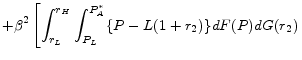
$\displaystyle \Pi_{A} = \beta(-Lr_{1}$		$\displaystyle +L(r_{1}+\alpha))$
		$\displaystyle +\beta^{2}\left[ \int_{r_{L}}^{r_{H}}\int_{P_{L}}^{P_{A}^{*}} \{ P-L(1+r_{2}) \} dF(P)dG(r_{2}) \right.$
		$\displaystyle \left. +\int_{r_{L}}^{r_{H}}\int_{P_{A}^{*}}^{P_{L}} \{ L(1+i) -L(1+r_{2}+\alpha)-L(1+r_{2})\} dF(P)dG(r_{2}) \right]$

where $\alpha$ is the margin on the adjustable rate mortgage contract. The value of house at which default occurs with an adjustable rate contract is $P_{A}^{*} = L(1+r_{2}+\alpha)$ . The first period profit for the lender is $-Lr_{1}+L(r_{1}+\alpha) = L\alpha$ . If the loan is paid off, the lender's profit is $L(1+r_{2}+\alpha)-L(1+r_{2}) = L\alpha$ , the same as the first period profit. If the borrower defaults, the profit would be $P-L(1+r_{2})$ . The expected profit from the second period is then $\int_{r_{L}}^{r_{H}}\int_{P_{L}}^{P_{A}^{*}} \{ P-L(1+r_{2}) \} dF(P)dG(r_{2}) +\int_{r_{L}}^{r_{H}}\int_{P_{A}^{*}}^{P_{L}} \{ L(1+r_{2}+\alpha)-L(1+r_{2})\} dF(P)dG(r_{2})$ .

Simplifying lenders' profits from a FRM contract and an ARM contract, we have

$\displaystyle \Pi_{F} = \beta L(i-r_{1}) - \frac{\beta^{2}L^{2}(1+i)^{2}}{2J} + \frac{\beta^{2}P_{H}L(1+i)}{J} - \frac{\beta^{2}P_{L}^{2}}{2J} - \beta^{2}L(1+E(r_{2}))$

and

$\displaystyle \Pi_{A} = \alpha\beta L - \frac{\beta^{2}L^{2}(1+E(r_{2})+\alpha)^{2}}{2J} + \frac{\beta^{2}P_{H}L(1+E(r_{2})+\alpha)}{J} - \frac{\beta^{2}P_{L}^{2}}{2J} - \beta^{2}L(1+E(r_{2})) - \frac{\beta L\sigma_{r}^{2}}{2J}$

where $J = P_{H} - P_{L}$ .

The profit for the FRM contract and the profit for ARM contract are the same, except for the last term in profit for the ARM contract, $\frac{\beta L\sigma_{r}^{2}}{2J}$ , which depends on the second period interest rate volatility. This term indicates that an ARM borrower can default not only due to low house price but also due to high interest rate (and consequently high payment size) in the second period ("payment shock"). While FRM borrowers default only when the house price is low since their second period payment is fixed, ARM borrowers can default due to large interest payments. Therefore, the value of a default option for an ARM borrower is a function of both interest rate volatility and house price volatility and higher than the default option for the FRM borrower. The augmented default option due to interest rate volatility should decrease the profit of the ARM lender, but not that of the FRM lender. Therefore, expected large volatility of interest rates would increase ARM margins charged by lenders. Note that the effect of interest rate volatility depends on the size of the loan, implying the option is more valuable for larger loans.

We assume that each mortgage contract is competitively offered so that expected profit from each contract is zero: $\Pi_{F}=0$ and $\Pi_{A}=0$ . This zero profit condition gives mortgage interest rates (FRM loans) and margins (ARM loans) for the given loan size:

$\displaystyle i^* = i(L,r_{1},E(r_{2}),P_{H},P_{L}) \textrm{ and } \alpha^* = \alpha(L,\sigma_{r}^{2},E(r_{2}),P_{H},P_{L})$

Note that the first period interest rate, , is a determinant of the FRM rate, , but not the ARM margin. Second period interest rate volatility, $\sigma_{r}^{2}$ , is a determinant of the ARM margin, $\alpha^*$ , but not the FRM rate. The first period interest rate only enters the FRM rate since the ARM margin is a spread over the interest rate and the ARM rate for the first period already fully reflects the first period interest rate. Therefore, the ARM margin is independent of the market interest rate in the first period and should be large only enough to cover fluctuations in the second period cash flow. Especially, since high volatility of the market interest rate in the second period will more likely lead to exercise of the default option by the borrower, the margin should be a positively related to interest rate volatility.

Another implication to note is that difference between the first period mortgage payment of a FRM and the first period payment for an ARM should be equal to (inverse of) the difference in the second period expected payoffs. For example, if an ARM loan is expected to have a higher payoff in the second period than a FRM loan, the first period payment from the ARM loan should be smaller than that of the FRM loan. This implication also allows us to write the difference in second period net profits as a function of the difference in the first period net profits. But since there are no defaults in the first period, the difference in the first period profits is the difference in first period payments. Then the difference in second period net profit is a function of the difference in first period payments.

2.3 Borrower's Problem

We assume borrowers in this economy are risk neutral. Expected utility from a fixed rate contract for a borrower is

$V_{F} = L-P_{0}-\delta Li+\delta^{2} \int_{r_{L}}^{r_{H}}\int_{P_{F}^{*}}^{P_{H}} \{ P-L(1+i) \} dF(P)dG(r)$ ,

where is the purchase price of the house and $\delta$ is the time discount factor of the borrower. Unlike the lender who borrows from the capital market only as much as it expects to lend to the borrower, the borrower is allowed to borrow more than the value of house. If the borrower borrows more than the value of house, the borrower will have a positive cash flow in the first period. At the end of the first period, the borrower makes the first payment for the loan, . At the end of the second period, if the house is valued more than the payoff amount of the loan, , the borrower pays off the loan and receives a return of . If the house is valued less than the amount owed, then the borrower defaults on the loan, and turns over the house to the lender. The borrower's return at the default is zero.

Similarly, expected utility from an adjustable rate contract for a borrower is

$V = L-P_{0}-\delta L(r_{1}+\alpha)+\delta^{2} \int_{r_{L}}^{r_{H}}\int_{P_{A}^{*}}^{P_{H}} \{ P-L(1+r_{2}+\alpha) \} dF(P)dG(r)$ ,

The first period payment for the borrower is $L(r_{1}+\alpha)$ , and the second period payment is $L(1+r_{2}+\alpha)$ . As in the fixed rate contract, the borrower will default when the house is valued less than the second period payment, and receives a return of zero. If the borrower repays the loan payoffs, the return would be $P-L(1+r_2+\alpha)$ . If the borrower defaults, the return would be zero. Note that the time discount factor of the borrower is $\delta$ , and we assume $\delta<\beta$ , implying that borrowers are less patient than lenders.

Simplification of the expected utilities yields

$\displaystyle V_{F} = L-P_{0}-\delta Li + \frac{\delta^{2}(P_{H}-L(1+i))^{2}}{2J}$

and

$\displaystyle V_{A} = L-P_{0}-\delta L(r_{1}+\alpha)+\frac{\delta^{2}}{2J} \{ (P_{H}-L(1+E(r_{2})+\alpha))^{2} + \delta^{2}L^{2}\sigma_{r}^{2} \}$

As with the lenders' profit from a FRM contract and an ARM contract, the main difference in expected utilities of loan contracts is the interest rate volatility, $\frac{\delta^{2}L^{2}\sigma_{r}^{2}}{2J}$ . It is obvious that the interest rate volatility has positive effects on a borrower's utility for the same reason it negatively affects ARM lenders' cash flows. Interest rate volatility decreases lenders' cash flows by $\frac{\beta^{2}L^{2}\sigma_{r}^{2}}{2J}$ , but it increases borrowers' expected utility by $\frac{\delta^{2}L^{2}\sigma_{r}^{2}}{2J}$ . If the lender and the borrower have the same time discount factor, these two effects will cancel each other. However, since the borrowers are more impatient than the lenders, $\delta<\beta$ . Thus, the value of the option is smaller for the borrower than for the lender, which means the net effect of the interest rate volatility would be negative for the borrower. In other words, when interest rate volatility rises, the lender raises the margins on the ARM contracts more than the borrower benefits from the default option.

2.4 Mortgage Contract Choice and Liquidity Constraints

In considering the theoretical model's predictions for borrowers' choice of mortgage instrument, we assume that instrument choice is independent of the loan size decision. The borrower decides first how much to borrow; and subsequently given the chosen loan amount, the borrower selects the most affordable instrument. This assumption likely is realistic in many cases: A borrower's available liquid assets determine the amount available for a down payment, or the borrower needs a specific amount of cash for debt consolidation or home improvements in a refinancing.⁴ Facing a binding equity requirement, liquidity-constrained borrowers would try to put as little as possible in down payment or to borrow as much as possible (Engelhardt and Mayer (1998)) and choose the contract that minimize loan costs.

The purpose of assuming independence of the loan size and mortgage instrument choices is to abstract from the many factors that affect borrowers' loan size decisions and focus on the relative cost of the two types of mortgage instruments at different levels of LTV.⁵ Note that the independence assumption does not imply that loan size is exogenous. It only implies that loan size decision and mortgage instrument choice are made separately. In the empirical work that follows, we remove this restrictive assumption and allow loan size (measured by LTV ratios) to be endogenous.

Proposition 1

For a given level of loan size, L, the mortgage rate for a fixed-rate contract is given by

$\displaystyle i = \frac{(J+\beta P_{H})-\sqrt{R_{F}}}{\beta L}$

where

$\displaystyle R_{F} = (J+\beta P_{H})^2 - \beta\{ 2LJ(1+r_{1}) + 2\beta LJ(1+E(r_{2})) + \beta P_{L}^{2} \},$

and the margin for an adjustable-rate contract is given by

$\displaystyle \alpha = \frac{(J+\beta P_{H})-\sqrt{R_{A}}}{\beta L}-1-E(r_{2}),$

where

$\displaystyle R_{A} = (J+\beta P_{H})^2 - \beta\{ 2LJ(1+\beta)(1+E(r_{2}))+\beta P_{L}^{2}+\beta L^{2}\sigma_{r}^{2} \}.$

Then, we have

$\displaystyle (1.1)$		$\displaystyle i < (\alpha + E(r_{2}))$
$\displaystyle (1.2)$		$\displaystyle \frac{di}{dr_{1}}<1$

Proof: See the appendix.

Note that for any loan size, the expected mortgage rate on an ARM contract in the second period is always higher than the mortgage rate on a FRM contract. However, this result does not necessarily imply that an ARM loan is more expensive than a FRM loan, since the ARM loan has a higher probability of default than the FRM loan. The expected payoff for lenders can be larger for FRM loans or for ARM loans depending on the default probabilities. The proposition above also implies that a response of a FRM mortgage rate for a change in the current interest rate is less than unity. Since a response of an ARM mortgage rate for a change in the current interest rate is always equal to unity by construction, the current interest rate always has larger effects on ARM loans than on FRM loans. Given the expected interest rate in the future, an increase in the current interest rate has a larger effect on the interest payment on ARM than on the interest payment on FRM loan.

Recall that we assume that borrowers are more impatient than lenders, which implies that two loans with the same (zero) expected profit might provide borrowers different expected utilities, and thus borrowers will choose the contract that generates higher expected utility.

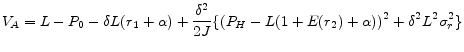
Proposition 2

The utility difference between an ARM contract and a FRM contract for a given loan size is given by

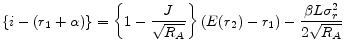
$\displaystyle dV = V_{A} - V_{F} = \delta L \{ i-(r_{1}+\alpha) \} \left[ 1-\frac{\delta}{\beta} \right].$

Proof: See the appendix.

The utility difference between two types of mortgage is determined by the difference in the discounted sum of mortgage payments. A borrower would prefer a mortgage loan that gives a lower present value of future payments. Proposition 2 indicates that two factors determine which mortgage contract is less costly: (1) the difference in mortgage payment in the first period, $L\{i-(r_{1}+\alpha)\}$ and (2) the difference in time discount factors, $\left[ 1-\frac{\delta}{\beta} \right]$ . If borrowers and lenders have the same time discount factor, $\delta=\beta$ , borrowers would be indifferent between FRM contracts and ARM due to a symmetric nature of borrowers' expected utility and lenders' expected profit: Loss (gain) by borrowers would be always equal to gain (loss) by lenders. All the loans offered have zero profit, and the expected utility of different loans is the same, which implies that borrowers should be indifferent between them. Throughout the analysis, since we assume that the borrower is less patient than the lender, $\delta<\beta$ , the first period mortgage payment decides the borrower's preference. Alternatively, note that the zero profit conditions imply second period payoffs are always proportional to the first period payoffs (with different signs), and one can express total discounted payoffs from two periods as a function of the first period payments only.

Proposition 3

Let $dV=V_{A}-V_{F}$ the utility difference between an ARM contract and a FRM contract.

(3.1) $\frac{\partial dV}{\partial L} \geq 0$ when the loan size L is small and $\frac{\partial dV}{\partial L} \leq 0$ when the loan size is large.

(3.2) $i>(r_{1}+\alpha)$ when is small, but $i<(r_{1}+\alpha)$ when is large.

(3.3) Mortgage rate difference, $\{i-(r_{1}+\alpha)\}$ , can be approximated as

$\displaystyle \{i-(r_{1}+\alpha)\} = \left\{ 1-\frac{J}{\sqrt{R_{A}}} \right\} (E(r_{2})-r_{1}) - \frac{\beta L\sigma_{r}^{2}}{2\sqrt{R_{A}}}.$

Proof: See the appendix.

Proposition 3 indicates that the mortgage type choice depends on the loan size itself (Figure 3). When the loan size is small, an increase in a loan size increases the interest payment of a FRM loan in the first period more than the interest payment of an ARM loan with the same loan size in the same period. An increase in loan size spreads increased payment equally over two periods for a FRM loan, but raises the second period payment disproportionally more (and the first period payment proportionally less) for an ARM loan. The difference in the first period payment and the second period payment for an ARM loan depends on difference between the current interest rate and the expected interest rate in the second period, or equivalently, on the slope of the yield curve or the term spread. In other words, the steeper the yield curve, the disproportionately larger the increase in the second period payment compared to the increase in the first period payment on an ARM loan. This implies that the slope of the yield curve plays a large role in a borrower's choice between an ARM loan and a FRM loan. The larger the expected interest rate in the second period compared to the current interest rate, the less costly is an ARM compared to FRM loans for borrowers.

The second part of Proposition 3 implies that borrowers' preferences change as the loan size increases. When the loan size is relatively small, the slope of yield curve is more important than interest rate volatility in borrowers' loan choice. As the loan size becomes larger, the effect of interest rate volatility grows, raising ARM margins due to potential payment shocks in the second period and ultimately making ARM contracts more expensive than FRM contracts. When the loan size is large enough, the first period payment of an ARM loan exceeds the first period payment of a FRM loan. The borrower finds ARM loans more costly and changes preferences in favor of a FRM loan. Therefore, as we have asserted in the introduction, borrowers' preference for ARM loans is not monotonic in loan size but rather humped shape. ARM loans are preferred as loan size increases but only up to a certain loan size. Once the loan becomes large enough, FRM contracts are preferred. The two factors underlying the humped shape of mortgage choice are term structure and volatility. A steeper term structure makes ARM contracts more attractive than FRM contracts, while a larger volatility of interest rate makes ARM contracts less attractive.

The third part of Proposition 3 makes this point more clear. One can approximate

$\displaystyle \beta L\{i-(r_{1}+\alpha)\} = -\sqrt{R_{F}} + \sqrt{R_{A}} + \beta L(E(r_{2})-r_{1}),$

from Proposition 1 to yield

$\displaystyle \{i-(r_{1}+\alpha)\} = \left\{ 1-\frac{J}{\sqrt{R_{A}}} \right\} (E(r_{2})-r_{1}) - \frac{\beta L\sigma_{r}^{2}}{2\sqrt{R_{A}}}$

It means that the difference in mortgage rates of two instruments in the first period depends on two factors, the slope of the yield curve, $(E(r_{2})-r_{1})$ , and the interest rate volatility, $\sigma_{r}^{2}$ . The effect of the first factor, the slope of the yield curve (term spread), which we call "the term structure effect," is given by $\left\{ 1-\frac{J}{\sqrt{R_{A}}} \right\}$ , while the effect of the second factor, the interest rate volatility, which we call "the interest rate volatility effect," is given by $\frac{\beta L}{2\sqrt{R_{A}}}$ . The Appendix shows that $\sqrt{R_{A}}$ is decreasing in loan size and bounded below by , which implies $\left\{ 1-\frac{J}{\sqrt{R_{A}}} \right\}$ is positive, but decreasing in loan size. Note that $\frac{\beta L}{2\sqrt{R_{A}}}$ is positive and increasing in loan size. Therefore, the term spread and the interest rate volatility have opposite and competing effects on mortgage rate differential. The balance between these two factors is determined by the loan size. Increasing loan size weakens the term structure effect but strengthen the interest rate volatility effect. Thus, when the loan size is small, the "term structure effect" makes ARM contracts less costly than FRM contracts and therefore preferable. But when the loan size is large, the "interest volatility effect" makes FRM contracts less costly and preferable to ARM contracts.

Proposition 4

Let $L^{*}$ satisfy $V_{A}(L^{*})=V_{F}(L^{*})$ so that $V_{A}(L^{*})>V_{F}(L^{*})$ for any $L < L^{*}$ , and $V_{A}(L^{*})<V_{F}(L^{*})$ for any $L > L^{*}$ . Then we have

(4.1)

$\displaystyle \frac{dL^{*}}{dE(r_{2})} > 0$

(4.2)

$\displaystyle \frac{dL^{*}}{d\sigma_{r}^{2}} < 0$

(4.3)

$\displaystyle \frac{dL^{*}}{dE(P)} > 0$

(4.4)

$\displaystyle \frac{dL^{*}}{d\sigma_{P}^{2}} < 0$

Proof: See the appendix.

Proposition 4 above shows the effects of credit and housing market conditions on loan choice. Let $L^{*}$ be the loan size at which a borrower is indifferent between an ARM contract and a FRM contract. For loans larger than $L^{*}$ , a borrower prefers FRM contracts; and for loans smaller than $L^{*}$ , the borrower prefers ARM contracts. An increase in expected interest rate in the second period shifts loan preference toward ARM contracts since it will amplify the term structure effects. The loan size would need to be relatively large for the interest volatility effects to dominate the term structure effects. An increase in interest rate volatility reduces the loan size $L^{*}$ at which FRM loans become preferable to ARM loans.

An increase in expected house prices increases the loan size level $L^{*}$ below which ARM contracts are preferable to FRM loans. This result is obtained because but a higher house prices in the second period reduce the expected probability of default on ARM loans. An increase in the volatility of house prices has the opposite effect on $L^{*}$ . Greater house price volatility increases the probability of default on ARM loans, making ARM loans more costly to borrowers than FRM loans in the first period and thus lowers the loan amount at which borrowers are indifferent between ARM and FRM loans.

3. Data

3.1 AFSA Subprime Mortgage Database

Data for this study are from the American Financial Services Association (AFSA) subprime mortgage database for the first quarter of 2006. The subprime mortgage subsidiaries of seven large financial institutions contributed to the database. The database includes all mortgages originations or purchases of these subprime mortgage companies. The AFSA subprime mortgage database accounts for a substantial share of all subprime or higher cost mortgages originated in the United States (Staten and Elliehausen 2001; Avery, Canner, and Cook 2005). Although the mortgages originated or purchased by these companies may not be representative of all subprime mortgages, particularly those originated by small lenders, mortgages in the AFSA subprime database likely are typical of subprime mortgages at large lenders. The variables in the dataset include loan terms (such as loan amount, interest rate and fees, term to maturity, and terms for interest rate adjustments), borrower characteristics (income, FICO risk score, age, sex, and race or ethnic background), and loan performance (historical and current delinquency, whether the loan was foreclosed, and delinquency status at close).

We consider first lien mortgages originated from the first quarter of 1998 through the first quarter of 2006. This time span includes periods of both rising and falling interest rates. Housing price changes vary substantially across geographic areas during this period, with some areas experiencing little if any price appreciation and others experiencing rapid growth in prices. Thus, the data provide considerable variation in credit and housing market conditions that influence choices.

Table 1 provides descriptive statistics for data from AFSA used in this paper. Average LTV ratios did not vary much during the data period, 1998-2006, fluctuating between 76 and 78 percent. Note that dispersion of the ratios (measured by standard deviation) was much higher during the first four years (19 percent) than was for the rest of the period (16 percent). The average age of all borrowers is about forty-eight, but the average age increased from forty-eight to fifty during the first six years, then subsequently dropped to forty-six. The borrowers with home-purchase loans are on average younger, more notably, each year. New borrowers of purchase loans are always younger than the borrowers in the previous year. The average age of borrowers with home-purchase loan during the first quarter of 2006 was forty. The average FICO score has also decreased from 607 to 590 during the first three years, but increased subsequently to reach 616 in 2006. Fees and points on fixed-rate mortgages are on average much higher than those of adjustable-rate mortgages. Due to a downward trend in fees on fixed-rate mortgages, the difference in fees decreased throughout the sample period. The share of home-purchase loans is smaller than the share of refinance loans, ranging 16% to 32%. The share of home-purchase loans fell during the initial years but then increased during the latter years. Brokers have played a large role in mortgage origination in our sample. The share of loans intermediated by brokers rose from 55% to almost 80% at the end of sample.

3.2 Construction of Variables

LTV is loan to value ratio of a loan and was computed based on the reported loan amounts and house values for each loan in the dataset. PURCHASE, OWNOCC and MALE are indicator variables that take the value of one when the loan is used for house purchase (as opposed to a refinanced loan), when the borrower uses the house for his or her residence, and when the primary borrower is a male, respectively. DIVORCE is annual divorce rate for each state estimated from Census data. MOBILITY is the outward mobility rate (number of residents who move out of the county divided by the total population) for each county based on 2000 census. MINORITY is an indicator variable for an African American or Hispanic borrower. COLLEGE is the ratio of residents who have completed college education or higher in each metropolitan area.

MHPR is the average house price appreciation over the past three years. We computed MHPR as quarterly price changes using metropolitan housing price index by OFHEO, averaged over the previous three years from origination quarter of a mortgage. VHPR is the volatility of house price changes over the previous three years, also based on OFHEO MSA index. BRP is bond term premium, advocated by Koijen, van Hemert and van Nieuwerburgh (forthcoming), as a strong predictor for mortgage choice, is calculated as five-year Treasury bond yield less the average one-year Treasury rate over the last three years. TERM is the term spread (or the slope of the yield curve) and calculated as a difference between 5 year Treasury rate and 1year Treasury rate in a month when the mortgage was originated. INTVOL is a measurement of interest rate volatility which we compute as a difference between the highest one year Treasury rate and the lowest one year Treasury rate over previous three years from the month of a loan origination (Figure 4). A traditional measure of interest rate volatility would be GARCH type, return based models, such as Longstaff and Schwartz (1992, 1993). But range based measures for interest rate volatility appears to be more appealing to us for following reasons. First, it is well known that GARCH based volatility measures can be highly inefficient in the presence of stochastic volatility due to non-Gaussian measurement errors (Alizadeh, Brandt and Diebold 2002). Second, GARCH type return based methods use only the end-of-period prices during the sample period, leaving out potential information contained in within-period price developments. Third, range based measures are much easier and convenient to compute than GARCH type of measures. Traders and investors have been using the information contained in range based measures through "candlestick plots" for years. Even for borrowers who are not quantitatively-sophisticated as professional traders, a past range of interest rate fluctuations is convenient to obtain and easy to understand.

4. Empirical Estimation and Results

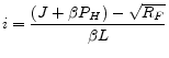
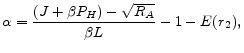
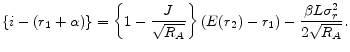
The main hypotheses of the model are given in Propositions 3 and 4. First, the model implies that a steeper slope of the yield curve makes ARM loans preferable to FRM loans, all else equal, while greater interest rate volatility makes FRM loans preferable to ARM loans. Second, for given slope of yield curve and interest rate volatility, loan size will be negatively related to choice of FRM loans when the loan size is small, but will be positively related to choice of FRM loans when the loan size is large. In the next two subsections, we test these hypotheses by estimating models predicting the (1) probability of choosing a FRM loan and (2) the FRM mortgage rate and ARM margin.

4.1 Probability of Choosing a FRM loan

In testing these predictions, first we estimate probit models for mortgage choice equations. If the mortgage rate of a FRM contract is given

$\displaystyle y_{t}^{F} = X_{t}'\beta^{F} + u_{t}^{F}$

and the mortgage rate of an ARM contract is

$\displaystyle y_{t}^{A} = X_{t}'\beta^{A} + u_{t}^{A}$

then, a FRM contract is preferred if

$\displaystyle y_{t} = y_{t}^{A} - y_{t}^{F} = X_{t}'\beta + u_{t} > 0$

where $\beta = \beta^{A} = \beta^{F}$ and $u_{t} = u_{t}^{A} - u_{t}^{F}$ .

Our theoretical model and previous research on mortgage contract choice provide guidelines for the selection of explanatory variables $X_{t}$ . Explanatory variables include loan to value, the slope of the yield curve, interest rate volatility, expected house price appreciation, and house price volatility.

Inclusion of loan to value (LTV) ratio in the probit regressions imposes some important econometric issues due to potential endogeneity of loan size. First of all, at least for some borrowers in the dataset, the down payment requirement may not be binding⁶, and loan size would be endogenous choice for them. Anecdotal evidence indicates that, especially for later years in the sample, many subprime lenders had quite loose loan limits primarily for certain borrowers who otherwise did not appear to be especially risky⁷. Second, even if the loan limit is binding, the loan limit may be imposed on individual basis and depend on observable and unobservable borrower characteristics. It is possible that some unobservable characteristics might be correlated with error terms in the rate equations above.

In any case, it is not necessary to assume exogeneity of LTV ratios in the probit regressions. To control for potential endogeneity of LTV ratios, we use a two step procedure by Newey (1987) which generates consistent estimates for parameters and standard errors in the regression in the presence of potentially endogenous regressors. The procedure also allows a direct test for exogeneity of LTV ratios in the regressions. For comparison, we also report the estimation results based on regular probit procedures without endogeneity correction.

Newey's two step procedure involves predicting LTV ratios on a set of instruments. In selecting proper instruments for LTV ratios, we follow Harrison, Noordewier and Yavas (2004), who examine optimal loan size choice questions in a signaling equilibrium framework. They show that, when default costs are high, risky borrowers might choose lower LTV loans. But when default costs are low, risky borrowers choose high LTV loans. Therefore, we assume that LTV ratios depend on default costs and future income prospect of borrowers, and include FICO scores, house price-income ratio and income growth rate for the metropolitan area of the borrower⁸.

We also consider two important factors for mortgage contract choice that were not considered in the theoretical model. The first is borrowers' risk aversion. As shown in Campbell and Cocco (2003), the degree of risk aversion can play an important role for mortgage instrument choice. Due to inherent interest rate risk embedded in ARM loans, borrowers with high degrees of risk aversion might prefer FRM loans while borrowers with low degrees of risk aversion might choose an ARM loan over a FRM loan. Another factor, emphasize by Brueckner (1992), is borrowers' propensity for mobility which has been documented as one of the most important factor for mortgage choice. Borrowers with high mobility more likely choose an ARM loan over a FRM loan to take advantage of low initial rates. But borrowers with lower mobility will choose a FRM loan over an ARM loan to take advantage of constant interest rate over longer periods.⁹ We use several variables reflecting borrower characteristics that are correlated with risk tolerance and mobility propensity. Some of the variables may be related to risk tolerance and mobility at the same time. However, since our interest is not to distinguish effects of risk-tolerance from borrower mobility in mortgage choice but to account the influence of such motives on choices, we do not attempt to separate two effects from estimation results.

Table 2 reports probit estimation results for the probability of FRM choice with endogeneity correction, and Table 3 reports probit estimation results without correction. To show compounding effects of loan size (measured by LTV) for explanatory variables on mortgage instrument choices, the sample is split into two subsamples: one with LTV ratios less than 80 percent (where the term structure effects are hypothesized to dominate) and another with LTV ratios larger than 95 percent (where interest rate volatility is expected to offset term structure effects) to differentiate the influence of loan size. Each regression model was estimated separately with each subsample. The model implies that interest rate volatility increases ARM spreads, making FRM contracts more affordable and preferable. Moreover, this effect compounds with loan size: volatility effect increases as loan size rises. Therefore, the coefficient on interest rate volatility should be larger with the subsample with high LTV ratios.

Specification 1 includes only information about local economic and demographic conditions such as the percentage of residents with college education or higher, state divorce rate, and unemployment rate. Specification 2 includes only borrower and loan characteristics. Specification 3 includes only term spread, interest rate volatility, average house price growth rate and volatility of house price growth rate. Specification 4 includes all the variables from Specification 1 through 3. Bond risk premium is used for term structure effects instead of term spread in Specification 4. In Specification 6, we include both term spread and interest rate volatility.

Overall, the results support Proposition 3 and 4, consistently across specifications having different sets of explanatory variables. From the Wald tests reported in the last row of the Table 2, the exogeneity of LTV is rejected in most specifications, often very strongly. Regardless of whether we correct for endogeneity, however, the results support the implications of the model that ARMs are more attractive than FRMs at lower LTV and that FRMs are more attractive than ARMs at high LTV, the coefficients are negative for subsamples with low LTV loans but positive for subsamples with high LTV loans. In both tables, the coefficients on LTV ratios are mostly statistically significant. Note that estimated coefficients are larger in absolute value in models that correct for endogeneity across all specification, which suggests that failure to address endogeneity of LTV in mortgage instrument choice results in underestimating the effect of LTV ratio on instrument choice.

The estimated coefficients on term spread are significant and negative in all estimated models. It confirms the model's prediction that steeper yield curves render ARM loans preferable. The coefficients on term spread are somewhat larger in absolute value for subsamples with high LTV loans than those for subsamples with low LTV loans. Thus, the term structure effect appears to be stronger when the loan is relatively large.

We also include the long-term bond risk premium, the spread between long term rate and expected short term rate. Koijen, Van Hemert and Van Nieuwerburgh (2009) advocate the long-term bond risk premium as the key determinant for mortgage instrument choice. They claim that the term spread is an imperfect predictor for the long-term bond risk premium and has an errors-in-variables problem. Specification 5 and Specification 6 of Table 2 presents probit regression results when the long-run bond risk premium is included¹⁰. When the term spread is replaced with the bond risk premium in Specification 5, the results are still very similar. The coefficient for the bond risk premium has the expected sign and is significant. In addition, consistent with the model predictions, the bond risk premium has smaller effects on mortgage instrument choice for a subsample with high LTV loans. Specification 6 includes both of the term spread and the bond risk premium. The coefficients on both variables are significant with the expected negative sign. And the both coefficients are smaller in absolute value when the LTV ratios are lower. These results indicate that neither of the variables dominates the other and that each of the bond risk premium and the term spread might only partially reflect the future expected short term interest rate. However, regardless of relative effectiveness between the term spread and the long term bond risk premium, they both support the model predictions: Higher future expected interest rates make ARM loans more attractive than FRM loans.

The estimated coefficients on interest volatility are also consistent with the model implications from high interest rate volatility raising ARM margins as loan size increases. Coefficients are significant, positive, and large for the subsample of loans with high LTV. On subsamples with low LTV loans, coefficients are relatively small but positive and insignificant in some specifications or negative and significant in other specifications. The substantially stronger positive effects of interest rate volatility in the high LTV subsample supports the model's prediction that the interest rate volatility makes ARMs less attractive to borrowers at higher levels of LTV. We find similar results when probit models are estimated without the endogeneity correction in Table 3. The coefficients are positive and significant even though difference between coefficients with different subsample is much smaller.

Housing market conditions (expected returns on housing and volatility) have the predicted effects on mortgage contract choice. Higher expected house price appreciation reduces the probability of choosing a FRM, while greater volatility in housing returns is associated with a higher probability of choosing a FRM. The coefficients are mostly significant and do not differ systematically in magnitude in the low and high LTV subsamples.

Effects of individual borrower characteristics and borrowers' location characteristics appear consistent across specifications only for low LTV loans. For high LTV loans, the estimated effects are not statistically significant in most case. Coefficients on the home-purchase loan indicator are mostly negative, which implies that the ARM contracts are more likely to be used for home-purchase mortgages, while FRM contracts are more likely to be used for refinance contracts. Mayer and Pence's (2008) finding that subprime mortgage originations are associated with fast growing housing markets with considerable new construction activities suggests one possibility. If new construction activities are concentrated on entry-level small and less expensive houses, purchase loan borrowers might disproportionately include fist time borrower who are relatively young, mobile, more risk tolerant but financially more constrained. Perhaps ARMs are more affordable than FRMs for such borrowers, and rises in income and house prices in the future allow them to afford to refinance using FRMs. Minority borrowers (African American, Hispanic or Native American borrowers) consistently and significantly prefer FRMs when LTV ratios are low. This pattern repeats for subsamples with high LTV loans, but the effect is now weaker and insignificant. The borrowers who use mortgage brokers tend to choose ARM loans mostly when LTV ratios are low. For subsamples with high LTV loans, there is not a discernable pattern of broker intermediation for mortgage instrument choice. Older borrowers consistently choose FRMs over ARMs in the subsamples with low LTV, which is possibly due to their financial strength, which can allow higher monthly payments, or life cycle factors, such as large family size with school age children.

Demographic characteristics associated with the geographic location of the mortgaged property also generally have statistically significant effects on mortgage instrument choice in the low LTV subsample. Borrowers located in areas with larger proportions of highly educated people tend to choose FRMs over ARMs in subsamples with low LTV loans. In subsamples with high LTV loans, the effect is statistically insignificant or relatively small. The level of education can have two contrasting effects on borrowers' choice of mortgage instruments. On one hand, better educated borrowers might tend to prefer FRMs because they have higher incomes than less well educated borrowers and can afford to avoid interest rate risk associated with ARM loans. On the other hand, highly educated borrowers might prefer ARMs since they are mobile due to higher marketability of their job skills (Dohmen (2005)). The results indicate that the first effect dominate in the subsamples with low LTV loans. State divorce rates have unexpected effects on loan choice. The divorce rate has often been used as an indicator of propensity to move in mortgage literature (Deng, Quigley, and Van Order (2000)). For our data, results suggest that the state divorce rate is unlikely to be associated with mobility. The estimated coefficients for divorce rate are mostly positive and significant across different specifications. Even when they are negative, they are either small or insignificant.¹¹ Unemployment rates tend to have negative effects: Borrowers in areas with high unemployment rate tend to choose ARMs over FRMs. As other location variables, unemployment rate has strong effects for subsamples with low LTV loans. For loans with high LTV ratios, the effect is reversed, but insignificant.

Overall, borrower and location characteristics are important factors affecting mortgage instrument choices, but the effects are strong and consistently observed only for loans with low LTV ratios. In contrast, term structure effects, interest rate volatility effects, expected returns and volatility in housing are consistently strong regardless of subsamples, specifications, and endogeneity correction.

4.2 FRM Interest Rate and ARM Margin

Another way to examine the implications from the model is directly to compare the effects of future expected interest rate, interest rate volatility, expected housing return and its volatility on mortgage rates themselves. Proposition 4 has four implications. First, a higher expected interest rate would have larger effects on FRM rates than on ARM margins. Second, higher interest volatility would have larger effects on ARM margins than on FRM rates. Third, a higher expected housing return would have larger effects on FRM rates than on ARM margins. Fourth, a higher housing return volatility would have larger effects on ARM margins than on FRM rates.

In principle, we can test these implications by comparing slope coefficients on interest rate variables and housing market variables from regression models of ARM margins and FRM rates:

$y_{t}^{F} = X_{t}'\beta^{F} + u_{t}^{F}$ , and $y_{t}^{A} = X_{t}'\beta^{A} + u_{t}^{A}$

Estimation of FRM rates and ARM margins is not straightforward and more complicated than the previous probit estimation due to following complications. The first complication is that we do not observe mortgage alternatives that borrowers have foregone. We only observe characteristics of the mortgage product the borrower decided to take. This leads to a classical case of sample selection problem, which can be accounted for by using inverse Mill's ratio in the regressions. Therefore, we estimate

$\displaystyle y_{t}^{F} = X_{t}'\beta^{F} + \rho \left( \frac{\varphi(\cdot)}{\phi(\cdot)} \right)^{F} + u_{t}^{F}$

and

$\displaystyle y_{t}^{A} = X_{t}'\beta^{A} + \rho \left( \frac{\varphi(\cdot)}{\phi(\cdot)} \right)^{A} + u_{t}^{A}$

where $\left( \frac{\varphi(\cdot)}{\phi(\cdot)} \right)^{F}$ and $\left( \frac{\varphi(\cdot)}{\phi(\cdot)} \right)^{A}$ are inverse Mills ratios corresponding to choice of a FRM loan and choice of an ARM loan. In calculating the Mills ratios, we use Specification 3 in the Table 2. The second complication is that some of the explanatory variables, especially LTV ratios, can be potentially endogenous and might be correlated with error terms, $u_{t}^{F}$ and $u_{t}^{A}$ , in the regression model. To handle this, we rely on instrumental variable regressions with the same set of the instruments used in the previous probit models. The third complication is that the regression models with simultaneous endogeneity problem and sample selection problem do not have readily available computing procedures for standard errors. One can possibly rely on full information maximum likelihood, but due to the number of equations involved, we rely on bootstrap methods.

The last complication comes from complexity of actual FRM contracts and ARM contracts in the data. In the model, we abstract any fees and points that borrower can pay to lower mortgage rates on FRM contracts or margins on ARM contracts. The effects of fees and points are not negligible. In our data, the average fees/points paid is about 2.4 percent of the loan balance for FRM contracts. Therefore, ignoring fees and points can lead to over-estimation or under-estimation of actual costs of FRM contracts¹². One possible way to handle this problem is to use fees and points as additional explanatory variable. However, it would create another problem of potential endogeneity of discount points¹³. Therefore, we use instead APR for FRM rates, which reflects both the contract rate and initial fees amortized over the loan term.

Fees and points are much less important for ARM contracts than for FRM contracts. On average, the fees/points in ARM contracts are only 0.97 percent of the initial balance. There is an additional complication for ARM contracts. Most of the ARM contracts in the dataset are of a "hybrid" nature in the sense that they offer a period with some fixed rates at the beginning of the contract. Most of hybrid loans in the dataset have initial periods with fixed rate for the first two years in the contract (often called "teaser rate" because the initial fixed rate may be lower than the fully indexed rate), a product often called "2/28." Presumably, borrowers in ARM contracts can substitute low teaser rates for larger margins, similar to borrower's decisions in point/rate in FRM contracts, which implies that teaser rates and margins might be jointly determined. To account for effects of teaser rates, we use six-month LIBOR and other loan characteristics as instruments for the following reasons. First, the six-month LIOBR is used since there is a salient trend in average teasers in ARM contracts over time that are quite closely related to the LIBOR. Figure 5 shows average teaser rates quite closely follow LIBOR six-month rates over time. The correlation between the series is 0.82. Second, in many contracts, teaser rates are not substantially lower than fully indexed rates: The average difference between teaser rates and the sum of LIBOR and margin (a mortgage rate a borrower would have paid if there is no teaser rate) is 0.4 percent in our data. Thus teaser rates did allow some borrowers to pay lower rates initially, possibly at the cost of higher margins, but the effects appear quite small on average. Therefore, effects of potential endogeneity of teaser rates appear rather small, and we use borrower and loan characteristics in addition to six-month LIBOR, to instrument teaser rates.

Tables 4 and 5 report estimation results. For regressors, we include the expected interest rate, interest rate volatility, expected housing return and its volatility in addition to LTV ratios and borrower characteristics such as the indicator variable for purchase loans, the indicator variable for broker-intermediated loans, and the indicator variable for minority borrowers. We also include short-term (six-month) Treasury yields for different reasons for FRM rates and ARM margins. For FRM rates, we include short-term rates following Proposition 1, which shows the current short term interest rate has effects only on FRM rate, but not on ARM margins. For ARM margins, we include short-term interest rates to control for initial teaser rates. We use the past three year average of one-year Treasury rates for expected future interest rates, EXINT. As in the bond risk premium variable used in the mortgage instrument model in Table 2 and 3, expected future interest rates are based the approach suggested by Koijen, Van Hemert and Van Nieuwerburgh (forthcoming). In Table 4, we correct for potential endogeneity of LTV ratios regressions, utilizing the same set of the instruments used to predict LTVs for mortgage instrument choice estimations in Table 2. Table 5 presents the results from the same specifications in Table 4, but without endogeneity corrections.

Results of estimation are as follows: First, LTV ratios are generally statistically significant and positively associated with FRM rates in both the low and high LTV subsamples. In contrast, LTV ratios are negatively associated with ARM margins in the low LTV subsample but not significant in the high LTV subsample. Regression results without endogeneity correction, reported in Table 5, show even weaker effects of LTV on rates and margins. In contrast to Table 4, the effects on ARM margins are weaker than on FRM rates regardless of the level of LTV ratios in Table 5. Overall, the effect of rising LTV ratio appears to have considerably different effects on FRM rates and ARM margins depending on endogeneity correction and subsamples.

The estimated coefficients on expected interest rates and interest rate volatility are statistically significant and consistent with the model predictions. In the endogeneity corrected models, higher expected interest rates are associated with significantly higher FRM rates in all but one of six LTV subsample/model specifications. Higher expected interest rates were associated with lower ARM margins in all LTV subsample/model specifications (although in two cases the negative coefficients were statistically insignificantly different from zero). In the models that did not correct for endogeneity, higher expected interest rates were associated with higher FRM rates and lower ARM margins, although the coefficients were not statistically significant in a few cases. Thus, the results provide strong evidence that higher expected interest rates make ARM loans more affordable FRMs more costly. We test the null hypothesis that the effect of higher expected future interest rate on the ARM margin is equal to or larger than that on the FRM rate for each specification and each subsample, assuming that error terms, $u_{t}^{F}$ and $u_{t}^{A}$ , are independent. The null hypothesis is strongly rejected for subsamples with low LTV loans. The same test with high LTV loans does not support rejection of the null hypothesis as strongly.

Higher interest rate volatility is associated with significantly higher ARM margins in all LTV subsample/model specifications. Higher interest rate volatility is generally associated with significantly lower FRM rates. In the two cases when the interest rate volatility coefficient in the FRM rate model was positive, the size of the estimated coefficient was considerably smaller than the size of the estimated coefficient from the comparable ARM margin model. Thus, results of estimation indicate that greater interest rate volatility raises the price of ARM loans relative to FRM loans, consistent with the prediction of our theoretical model. We also test the null hypothesis that the effect of higher interest rate volatility on the FRM rate is equal to or larger than that on the ARM margin for each specification and each subsample, assuming that error terms, $u_{t}^{F}$ and $u_{t}^{A}$ , are independent. The result of the test confirms that the null hypothesis is strongly rejected for each specification and for each subsample, confirming differential effects of interest volatility on FRM rates and on ARM margins. Table 5, which reports the estimation results without endogeneity correction, shows similar results.

The estimation results with expected housing returns and volatility are not as consistent as interest rate variables. Proposition 4 shows that expected housing returns have larger effects on FRM rates than on ARM margins while housing return volatility appear to have larger effects on ARM margins, which implies that ARM loans are more affordable in growing housing markets, but FRM loans are better instruments in more volatile housing markets. For both of expected housing returns and volatility, the null hypotheses are rejected with low LTV subsamples, indicating that those implications are consistent only with low LTV loans. One possible reason for these weak results can be due to the fact that our measure of housing returns (and volatility) is based on metropolitan areas' aggregate indices. First, at least some metro regions are too large and contain very different submarkets so that returns based on the aggregate housing index is too imprecise to be used for individual housing returns. Second, the OFHEO indices, in particular, used for this study, might be slow in capturing changes in market valuations because indices are largely based on refinance mortgages rather than purchase mortgages.

Overall, the empirical results in this section provide very strong support for the role of interest rate volatility and expected interest rates but much weaker support for the role of expected housing returns and its volatility. The implications of the results on interest rate expectations and volatility are quite clear. Interest rate expectations and volatility are the major factors affecting the cost of mortgage instruments and help explain the nonlinear and hump-shaped mortgage choice decisions of Figure 1.

5. Conclusion

This paper investigates a classical mortgage choice question with new evidence in a new market environment, the subprime mortgage market, which emerged during the last decade and promoted new types of adjustable rate mortgages over a broad range of credit risks. Subprime mortgages were directed toward borrowers with greater risks of various types and constraints on further borrowing from prime sources. One interesting question raised in this paper is how these characteristics of borrowers influence mortgage choice. Contrary to a popular belief, we present evidence that choice of type of interest rate is hump-shaped--not monotonic--in loan size. A fixed-rate mortgage contract is the preferred choice when loan size, measured by LTV ratio, is small. As LTV ratio increases, borrowers become more likely to choose adjustable rate mortgage contracts. However, when LTV reaches a certain level (perhaps as high as 95 percent), borrowers start to switch back to fixed rate contracts. For these high LTV loans, fixed rate mortgages dominate borrowers' choice.

We present a very simple model that explains this "nonlinear" mortgage instrument choice. In a risk neutral world where lenders competitively offer both types of mortgage loans to borrowers who exercise a default option, mortgage instrument choice is determined by the first period mortgage payment. Borrowers choose whichever mortgage offers the lower first period payment. The model shows that the first period difference depends on two opposing effects: "term structure" effect and "interest rate volatility" effect. When the loan size is small, the term structure effect dominates: rising LTV ratios tend to raise FRM rates more than ARM margins, rendering ARM loans more attractive. However, when the loan size is large, the interest volatility effect dominates: rising LTV ratios increase ARM margins more, making FRM loans preferable. This leads to borrowers, starting with FRM loans for relatively small loans, to switch to ARM loans as loans become larger, but then convert back to FRM loans when loan size is extremely large.

We present empirical evidence in support of the model predictions. First, we examine directly borrowers' mortgage instrument choice in the probit framework. The results show that larger term spreads make ARM loans preferable, but high interest rate volatility makes FRM loans preferable, consistent with the model's predictions. Second, we also examined determinants of the FRM mortgage rates and ARM margins. Consistent with the model and the evidence from mortgage choices, higher expected future interest rate decrease ARM margins more than FRM rates, while an increase in interest rate volatility raises ARM margins more than FRM rates. This result holds regardless of sample selection, endogeneity in choice of instruments and relative loan size, and the inclusion of other explanatory variables in the model.

The effects of term spreads and interest rate volatility are strong and consistent across different specifications. The effects of other variables, such as expected housing returns, housing return volatility, borrower characteristics and loan characteristics, are not as consistent across specifications, though they generally support existing theories and intuitions for the subsample with low LTV loans. The results with high LTV loans are less consistent and often difficult to interpret. We believe that subprime borrowers are quite heterogeneous. In particular, borrowers with high LTV loans may quite different from credit-impaired lower LTV borrowers, which account for most of the subprime market.

Reference

Alizadeh, Sassan, Michael W. Brandt, and Francis X. Diebold (2002) "Range-Based Estimation of Stochastic Volatility Models," Journal of Finance 57, 1047-1091.

Ambrose, Brent and Anthony Sanders (2005) "Legal Restrictions in Personal Loan Markets," Journal of Real Estate Finance and Economics, 30 (2), 133-151.

Ambrose, Brent, Anthony Sanders, and Michael LaCour-Little (2004) " The Effect of Conforming Loan Status on Mortgage Yield Spreads: A Loan Level Analysis," Real Estate Economics, 32(4), 541-569.

Avery, Robert, Glenn B. Canner, and Robert E. Cook (2005). "New Information Reported

Under HMDA and Its Application in Fair Lending Enforcement," Federal Reserve Bulletin

(Summer 2005): 344-394.

Brueckner, Jan (1992) "Borrower mobility, self-selection, and the relative prices of fixed- and adjustable-rate mortgages," Journal of Financial Intermediation, 2(4), 401-421.

Brueckner, Jan. (1994) "Borrower Mobility, Adverse Selection and Mortgage Points," Journal

of Financial Intermediation, 3(4), 416-441.

Brueckner, Jan, and James Follain (1988) "The Rise and Fall of the ARM: An Econometric Analysis of Mortgage Choice", Review of Economics and Statistics, 70, 93-102.

Campbell, John Y., and Joao F. Coco (2003) "Household Risk Management and Optimal Mortgage Choice," Quarterly Journal of Economics, 118(4), 1449-1494.

Chari, V. V. and Ravi Jagannathan. (1989) "Adverse Selection in a Model of Real Estate Lending," Journal of Finance, 44, 499-508.

Dhillon, Upinder S., James Shilling, and C.F. Sirmans. (1987). "Choosing Between Fixed and

Adjustable Rate Mortgages," Journal of Money, Credit, and Banking 19, 260-267.

Dohmen, Thomas. (2005) "Housing, mobility and unemployment," Regional Science and Urban Economics, 35, 305-325.

Dunn, Kenneth and Chester Spatt. (1988) "Private Information and Incentives: Implications for

Mortgage Contract Terms and Pricing," Journal of Real Estate Finance and Economics, 1,

47-60.

Engelhardt, Gary. (1996) "Consumption, Down Payment, and Liquidity Constraints," Journal of Money, Credit, and Banking 28, 255-271.

Engelhardt, Gary and Christopher Mayer. (1998) "Intergenerational Transfers, Borrowing Constraints, and Saving Behavior: Evidence from the Housing Market," Journal of Urban Economics, 44, 135-157.

Fortowsky, Elaine, Michael LaCour-Little, Eric Rosenblatt and Vincent Yao (forthcoming) "Housing Tenure and Mortgage Choice" Journal of Real Estate Finance and Economics.

Goldberg, L. and Heuson, A.J., (1992) "Fixed vs. Variable Rate Financing: The Influence of Borrower, Lender and Market Characteristics," Journal of Financial Services Research, 6 (1), 49-60.

Harrison, David, Noordewier, T. and Yavas A. (2004) "Do Riskier Borrowers Borrow More?" Real Estate Economics, 32 (3), 385-411.

Iacoviello, Matteo. (2005) "House Prices, Borrowing Constraints and Monetary Policy in the Business Cycle," American Economic Review 95, 739-764.

Koijen Ralph, Otto van Hemert and Stijn van Nieuwerburgh (forthcoming) "Mortgage Timing," Journal of Financial Economics.

Longstaff, Francis A. and Eduardo S. Schwartz. (1992) "Interest Rate Volatility and the Term Structure: A Two-Factor General Equilibrium Model." The Journal of Finance, 47, 1259-1282.

Longstaff, Francis A. and Eduardo S. Schwartz. (1993) "Interest Rate Volatility and Bond Prices." Financial Analysts Journal, 49, 70-74.

Mayer, Christopher J. and Pence, Karen M. (2008) "Subprime Mortgages: What, Where, and to Whom?" NBER Working Paper No. W14083.

Newey, Whitney (1987) "Efficient estimation of limited dependent variable models with endogenous explanatory variables" Journal of Econometrics, 36, 230-251.

Ortalo-Magné, François and Sven Rady. (1999) "Boom in, bust out: Young households and the housing price cycle," European Economic Review, 43, 755--766.

Ortalo-Magné, François and Sven Rady. (2006) "Housing Market Dynamics: On the

Contribution of Income Shocks and Credit Constraints," Review of Economic Studies 73, 459-485.

Posey, Lisa and Abdullah Yavas. (2001) "Adjustable and Fixed Rate Mortgages as a Screening Mechanism for Default Risk," Journal of Urban Economics, 49(1), 54-79.

Stanton, Richard and Nancy Wallace. (1998) "Mortgage Choice: What's the Point?", Real Estate Economics 26, 173-205 Sa-Aadu, J., and C.F. Sirmans (1995). "Differentiated Contracts, Heterogenous Borrowers and the Mortgage Choice Decision," Journal of Money, Credit, and Banking, 27, 498-510.

Staten, Michael. and Gregory Elliehausen. (2001). "The Impact of the Federal Reserve Board's Proposed Revisions to HOEPA on the Number and Characteristics of HOEPA Loans," Working Paper, Georgetown University, Credit Research Center.

Stein, Jeremy. (1995) "Prices and Trading Volume in the Housing Market: a Model with Down Payment Effects," Quarterly Journal of Economics, 110, 379-406.

Titman, Sheridan (1992) "Interest Rate Swaps and Corporate Financing Choices," Journal of Finance, 47(4), 1503-16.

Tucker, Michael (1991) "Comparing Present Value Cost Differentials between Fixed and Adjustable Rate Loans: A Mortgage Simulation," Financial Review, 26(3), 447-458.

Accessible Version

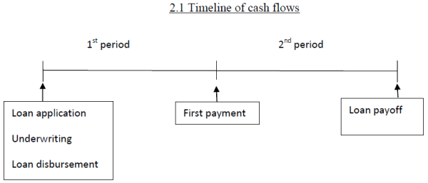
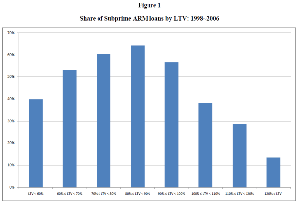
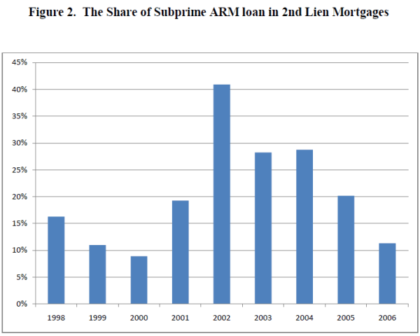
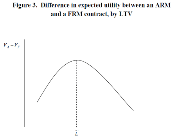
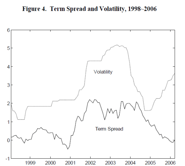
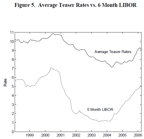
Table 1. Characteristics of Subprime Loans, Q1 1998-Q1 2006

	1998	1999	2000	2001	2002	2003	2004	2005	2006
LTV	76%	77%	77%	78%	76%	77%	78%	78%	77%
LTV: standard deviation	-18%	-19%	-21%	-20%	-17%	-15%	-16%	-16%	-15%
Borrower Age (all)	48	48	49	49	50	50	47	46	46
Borrower Age (all): standard deviation	-11	-11	-11	-11	-11	-12	-12	-12	-11
Borrower Age (purchase)	44	44	43	42	42	43	40	40	40
Borrower Age (purchase): standard deviation	-11	-10	-10	-10	-11	-11	-11	-11	-10
FICO	607	598	590	597	600	609	615	620	616
FICO: standard deviation	-66	-63	-62	-60	-62	-62	-62	-64	-65
Fees/Points (FRM)	3.45%	3.30%	3.37%	2.87%	2.51%	1.80%	1.59%	1.75%	2.02%
Fees/Points (FRM): standard deviation	-2.70%	-2.50%	-2.50%	(2. 7%)	-2.50%	-2.10%	-1.90%	(1. 8%)	-1.70%
Fees/Points (ARM)	0.61%	1.17%	1.10%	1.01%	0.94%	0.97%	1.01%	0.94%	0.86%
Fees/Points (ARM): standard deviation	-2.10%	-2.00%	-2.30%	-2.10%	-2.00%	-1.80%	-1.80%	-1.80%	-1.70%
Purchase	26%	22%	16%	17%	17%	20%	26%	29%	32%
Broker	55%	54%	48%	58%	68%	71%	68%	69%	78%

Note: This table provides average of LTV, borrower age, FICO scores, fees and points as a percentage of loan amount for fixed rate mortgages, fees and points as a percentage of loan amount for adjustable rate mortgages, the share of purchase loans, and the share of broker intermediated loans. The numbers in the parentheses for LTV, borrower age, FICO and fees are standard deviations.

Table 2. Mortgage Contract Choice: Probit Regression for FRM Contracts with Correction for Endogeneity of LTV

	Specification 1, LTV < 0.8	Specification 1, LTV > 0.95	Specification 2, LTV < 0.8	Specification 2, LTV > 0.95	Specification 3, LTV < 0.8	Specification 3, LTV > 0.95	Specification 4, LTV < 0.8	Specification 4, LTV > 0.95	Specification 5, LTV < 0.8	Specification 5, LTV > 0.95	Specification 6, LTV < 0.8	Specification 6, LTV > 0.95
LTV	-19.1556	6.63	-28.5155	16.1349	-16.8959	6.4183	-24.9449	-11.0606	-19.5908	118.0131	-22.7504	83.9909
LTV: t-statistics	-62.22	-28.97	-16.48	-1.38	-72.77	-38.62	-15.58	-0.79	-15.5	-1.86	-15.25	-1.92
TERM					-0.085	-0.1924	-0.1043	-0.1648			-0.0822	-0.1559
TERM: t-statistics					-24.27	-32.61	-9.28	-15			-7.43	-2.7
BRP									-0.1989	-0.1429	-0.1443	-0.2091
BRP: t-statistics									-10.83	-0.68	-6.52	-1.35
INTVOL					0.0636	0.1178	0.0158	0.2473	-0.0589	0.9393	-0.0311	0.7845
INTVOL: t-statistics					-20	-20.77	-1.06	-2.85	-5.86	-2.22	-2.59	-2.55
MHPR					-22.7771	-17.4563	-44.8827	-42.4685	-32.3432	41.2521	-37.6434	22.5066
MHPR: t-statistics					-71.91	-20.51	-21.43	-4.96	-15.45	-1.28	-15.22	-1.03
VHPR					6.5487	16.2513	21.6292	26.1345	18.2746	-8.0427	18.105	-5.5767
VHPR: t-statistics					-10.28	-14.32	-8.34	-5.69	-8.24	-0.46	-7.19	-0.43
PURCHASE			1.6973	-0.5675			-0.0225	-0.0247	-0.0192	0.0048	-0.0208	-0.0018
PURCHASE: t-statistics			-12.27	-8.24			-13.9	-7.33	-14.13	-0.34	-13.37	-0.18
MINORITY			0.253	0.016			0.1328	0.0423	0.0841	0.0684	0.1091	0.0627
MINORITY: t-statistics			-8.44	-0.34			-9.7	-3.41	-7.19	-0.9	-7.97	-1.13
BROKER			0.7265	0.3736			-0.1519	-0.239	-0.1091	0.0632	-0.1205	0.0214
BROKER: t-statistics			-13.15	-1.35			-16.53	-8.01	-11.76	-0.72	-11.33	-0.35
AGE			-0.042	0.0102			0.9887	-0.6658	0.7059	-0.2173	0.8818	-0.331
AGE: t-statistics			-11.79	-8.07			-8.92	-9.27	-8.43	-0.6	-9.02	-1.29
COLLEGE	-0.0129	-0.0128					0.4007	0.2062	0.2943	-0.4088	0.3472	-0.269
COLLEGE: t-statistics	-25.96	-15.86					-11.65	-3	-10.23	-1.4	-10.41	-1.33
DIVORCE	0.0879	-0.0188					1.0537	-0.109	0.8207	2.6046	0.9576	1.8469
DIVORCE: t-statistics	-20	-2.73					-15.82	-0.38	-15.29	-1.94	-15.1	-2.02
UNEMPLOY-MENT	0.0162	-0.0455					-0.0336	0.0119	-0.023	0.0014	-0.0289	0.0047
UNEMPLOY-MENT: t-statistics	-5.33	-6.57					-10.58	-7.96	-9.18	-0.17	-9.81	-0.86
No. of obs	569732	76822	175901	32565	760753	87338	119933	27148	119933	27148	119933	27148
Wald Test (Χ²(K))	5079.15	3849.16	1293.39	720.2	10012.82	5819.2	2125.87	2719.61	4174.56	132.3	3340.78	260.5
Wald Test Exogeneity	16610.47	590.81	3079.87	3.31	17530.33	1021.75	1685.84	0.88	1086.42	160.78	1363.34	86.87

Note: This table presents probit estimation results for FRM loan choice with endogeneity correction for LTV. The Χ² statistics for testing exogeneity by Newey (1989) are reported in the last row (with p-values in parenthesis). The columns with "LTV<0.8" provide estimation results with subsample with LTV lower than 80 percent, and the columns with "LTV>0.95" provide estimation results with subsample with LTV higher than 95%. Explanatory variables for probit regressions are LTV (loan to value ratio), TERM (term spread in percentage), BRP (bond risk premium in percentage), INTVOL (interest rate volatility in percentage), MHPR (average house price growth rate in decimal), VHPR (variance of house price growth in decimal), PURCHASE (dummy for purchase loan), MINORITY (African-American, Native American or Hispanic borrowers), BROKER (mortgage broker intermediated loan), AGE (borrower age), COLLEGE (the ratio of college or higher degree in the county), DIVORCE (state divorce rate), UNEMPLOYMENT (unemployment rate of MSA areas). t-statistics are provided in parentheses. Instruments for LTV include FICO, house price-income ratio and local income growth rate.

Table 3. Mortgage Contract Choice: Probit Regression for FRM Contract without Correction for Endogeneity of LTV

	Specification 1, LTV < 0.8	Specification 1, LTV > 0.95	Specification 2, LTV<0.8	Specification 2, LTV > 0.95	Specification 3, LTV<0.8	Specification 3, LTV > 0.95	Specification 4, LTV<0.8	Specification 4, LTV > 0.95	Specification 5, LTV<0.8	Specification 5, LTV > 0.95	Specification 6, LTV<0.8	Specification 6, LTV > 0.95
LTV	-1.6783	1.9351	-0.6537	0.3049	-1.7001	1.943	-0.8278	0.2962	-0.7225	0.1278	-0.7272	0.1424
LTV: t-statistics	-139.12	-49.67	-28.84	-3.21	-163.74	-52.95	-29.4	-2.73	-25.25	-1.15	-25.41	-1.27
TERM					-0.0792	-0.2242	-0.0959	-0.1677			-0.0361	-0.0877
TERM: t-statistics					-46.24	-44.7	-23.39	-18.81			-8.52	-9.51
BRP									-0.3973	-0.5021	-0.3886	-0.4805
BRP: t-statistics									-73.19	-43.49	-70.3	-40.78
INTVOL					0.0583	0.1208	0.1509	0.3174	-0.0131	0.1625	0.0026	0.202
INTVOL: t-statistics					-37.49	-24.66	-36.37	-32.11	-3.01	-16.73	-0.55	-19.13
MHPR					-19.461	-30.4888	-19.9422	-35.6402	-6.2039	-15.9011	-6.6219	-17.187
MHPR: t-statistics					-126.07	-49.02	-40.21	-26.77	-11.65	-11.26	-12.38	-12.1
VHPR					16.8083	25.869	4.4404	22.8818	0.731	12.607	-0.6441	10.6031
VHPR: t-statistics					-55.75	-27.14	-5.22	-11.93	-0.85	-6.28	-0.74	-5.25
PURCHASE			-0.4709	-0.6298			-0.01	-0.0222	-0.0081	-0.0164	-0.008	-0.0167
PURCHASE: t-statistics			-49.27	-16.46			-19.37	-18.77	-15.5	-13.56	-15.28	-13.79
MINORITY			-0.0772	0.0717			0.0425	0.047	-0.0041	-0.0027	0.0004	0.0059
MINORITY: t-statistics			-11.76	-4.43			-9.44	-4.99	-0.89	-0.28	-0.09	-0.61
BROKER			-0.0761	0.0025			-0.1003	-0.2155	-0.0251	-0.0628	-0.024	-0.066
BROKER: t-statistics			-11.07	-0.08			-32.08	-28.83	-7.49	-7.65	-7.14	-8
AGE			0.0129	0.0115			-0.605	-0.6263	-0.4821	-0.5861	-0.4917	-0.5889
AGE: t-statistics			-44.74	-17.7			-50.84	-14.05	-39.98	-12.91	-40.6	-13.02
COLLEGE	-0.0144	-0.0193					0.0049	0.1531	-0.0375	0.075	-0.0385	0.0749
COLLEGE: t-statistics	-65.77	-30.33					-0.6	-8.17	-4.5	-3.89	-4.61	-3.89
DIVORCE	0.0464	0.0435					0.1167	0.1225	0.0729	0.155	0.0789	0.1257
DIVORCE: t-statistics	-24.44	-8.16					-12.97	-3.25	-7.99	-4.04	-8.61	-3.28
UNEMPLOY-MENT	-0.0275	-0.1583					0.0116	0.0109	0.0122	0.0124	0.0122	0.0125
UNEMPLOY-MENT: t-statistics	-21.48	-42.84					-33.12	-14.82	-34.38	-16.59	-34.39	-16.68
No. of obs	569732	76822	175901	32565	760753	87338	119933	27148	119933	27148	119933	27148
LR (Χ²(K))	25593.82	7038.73	10981.05	1333.36	45586.8	9321.72	13771.79	4019.36	18894.9	5713.31	18967.41	5803.94
Pseudo R²	0.0327	0.0666	0.0474	0.0309	0.0438	0.0774	0.0861	0.1112	0.1182	0.158	0.1186	0.1605
Log-likelihood	-379112	-49336.4	-110230	-20914.6	-497646	-55591.4	-73075.3	-16067.8	-70513.7	-15220.8	-70477.5	-15175.5

Note: This table presents probit estimation results for FRM loan choice without endogeneity correction for LTV. The columns with "LTV<0.8" provide estimation results with subsample with LTV lower than 80 percent, and the columns with "LTV>0.95" provide estimation results with subsample with LTV higher than 95%. Explanatory variables for probit regressions are LTV (loan to value ratio), TERM (term spread in percentage), BRP (bond risk premium in percentage), INTVOL (interest rate volatility in percentage), MHPR (average house price growth rate in decimal), VHPR (variance of house price growth in decimal), PURCHASE (dummy for purchase loan), MINORITY (African-American, Native American or Hispanic borrowers), BROKER (mortgage broker intermediated loan), AGE (borrower age), COLLEGE (the ratio of college or higher degree in the county), DIVORCE (state divorce rate), UNEMPLOYMENT (unemployment rate of MSA areas). t-statistics are provided in parentheses.

Table 4. FRM Rate and ARM Margin Determination: With Correction for Endogeneity and Sample Selection Bias

	Specification 1, LTV < 0.8, FRM Rate	Specification 1, LTV < 0.8, ARM Margin	Specification 1, LTV > 0.95, FRM Rate	Specification 1, LTV > 0.95, ARM Margin	Specification 2, LTV < 0.8, FRM Rate	Specification 2, LTV < 0.8, ARM Margin	Specification 2, LTV > 0.95, FRM Rate	Specification 2, LTV > 0.95, ARM Margin	Specification 3, LTV < 0.8, FRM Rate	Specification 3, LTV < 0.8, ARM Margin	Specification 3, LTV > 0.95, FRM Rate	Specification 3, LTV > 0.95, ARM Margin
LTV	54.9932	-67.6855	100.1826	71.2832	49.1341	-47.9198	15.258	234.3466	95.5635	-54.9539	-1.431	0.7724
LTV: t-statistics	-20.2	-45.64	-2.47	-0.9	-21.42	-41.35	-3.05	-1.19	-9.8	-6.02	-0.4	-0.06
EXINT	0.4674	-0.569	-0.2386	-1.9726	0.4943	-0.7582	0.4533	-4.818	0.4993	-0.2738	0.5199	-0.304
EXINT: t-statistics	-19.41	-32.82	-0.72	-1.37	-19.78	-35.56	-17.21	-1.41	-13.02	-15.3	-29.09	-1.87
INTVOL	0.1656	0.3393	-1.2959	1.1869	0.1269	0.4566	-0.4501	1.3167	-0.4516	0.3968	-0.216	0.5777
INTVOL: t-statistics	-4.18	-15.32	-3.06	-4.31	-3.57	-22.87	-6.75	-4.64	-9.49	-25.9	-4.21	-5.19
MHPR					0.4222	-60.5518	20.5733	206.3661	155.87	-58.2891	-14.6309	1.9347
MHPR: t-statistics					-0.12	-26.71	-1.83	-1.14	-7.62	-5.56	-1.97	-0.1
VHPR					-10.9444	5.2781	-11.8662	-260.9205	-137.23	23.2732	10.6453	-6.5625
VHPR: t-statistics					-2.56	-1.93	-1.43	-1.17	-8.27	-3.14	-2.13	-0.3
PURCHASE									-6.0474	2.1426	0.2683	0.3316
PURCHASE: t-statistics									-9.37	-4.99	-1.23	-0.69
MINORITY									-1.3695	0.4746	0.3139	0.034
MINORITY: t-statistics									-6.08	-6.79	-7.16	-0.34
BROKER									-8.2796	2.0789	-1.0031	2.183
BROKER: t-statistics									-10.91	-10.44	-13.73	-8.5
SHORT	0.2716	0.3903	-0.4358	0.615	0.2669	0.4967	0.0176	0.7785	-0.4076	0.3306	0.1351	0.1888
SHORT: t-statistics	-10.41	-36.48	-1.91	-6.07	-11.4	-42.58	-0.46	-2.55	-6.58	-19.35	-4.81	-2.5
IMILLS	-4.3993	-4.0201	-9.268	2.028	-3.935	-2.8404	-1.4468	11.5061	-7.8773	-3.1527	0.1836	0.1543
IMILLS: t-statistics	-20.45	-44.96	-2.44	-0.55	-22.05	-42.3	-3.07	-1.08	-9.93	-6.11	-0.52	-0.11
EXINT: β_FRM≥β_ARM	34.9284	34.9284	1.1736	1.1736	38.1281	38.1281	1.5426	1.5426	18.2685	18.2685	5.0377	5.0377
INTVOL: β_FRM≤β_ARM	3.827	3.827	4.9149	4.9149	8.087	8.087	6.061	6.061	16.9706	16.9706	6.47572	6.47572
No. of obs	46231	51904	10418	4904	46231	51904	10418	4904	46231	51904	10418	4904
Waid (Χ²(K))	2683.64	3030.94	1312.5	690.29	4280.23	3102.67	6075.84	143.79	1359.76	5256.76	6046.02	8454.15
Root MSE	5.6014	3.2564	3.218	2.8316	5.0742	2.3933	1.2369	7.2867	7.9834	2.259	1.1932	1.1454

Note: This table presents instrumental variable regression results for FRM rate and ARM margins with endogeneity correction for LTV and sample selection bias correction. The columns with "LTV<0.8"provide estimation results with subsample with LTV lower than 80 percent, and the columns with "LTV>0.95" provide estimation results with subsample with LTV higher than 95%. Explanatory variables are LTV (loan to value ratio), EXINT (expected interest rate in percentage), BRP (bond risk premium in percentage), INTVOL (interest rate volatility in percentage), MHPR (average house price growth rate in decimal), VHPR (variance of house price growth in decimal), PURCHASE (dummy for purchase loan), MINORITY (African-American, Native American or Hispanic borrowers), BROKER (mortgage broker intermediated loan), SHORT (short term interest rate) and IMILLS (inverse mills ratio). t-statistics are provided in parentheses. EXINT is computed as past three year average of one-year Treasury rates, based the approach suggested by Koijen, Van Hemert and Van Nieuwerburgh (forthcoming). The sample selection bias is corrected by including inverse Mills ratio, which is in turn computed from instrumental variable probit regression from Table 2 (Specification 3). Instruments for LTV include FICO, house price-income ratio and local income growth rate. EXINT: β_FRM≤β_ARM reports t-statistics from testing EXINT coefficient on FRM rate is equal to or smaller than that on ARM margin. INTVOL: β_FRM≥β_ARM reports t-statistics from testing INTVOL coefficient on FRM rate is equal to or larger than that on ARM margin. MHPR: β_FRM≤β_ARM reports t-statistics from testing MHPR coefficient on FRM rate is equal to or smaller than that on ARM margin. VHPR: β_FRM≥β_ARM reports t-statistics from testing EXINT coefficient on FRM rate is equal to or larger than that on ARM margin. The tests on size of parameters assume error terms in two equations are independent, and follow normal distributions.

Table 5. FRM Rate and ARM Margin Determination: With Correction for Sample Selection Bias Only

	Specification 1, LTV < 0.8, FRM Rate	Specification 1, LTV < 0.8, ARM Margin	Specification 1, LTV > 0.95, FRM Rate	Specification 1, LTV > 0.95, ARM Margin	Specification 2, LTV < 0.8, FRM Rate	Specification 2, LTV < 0.8, ARM Margin	Specification 2, LTV > 0.95, FRM Rate	Specification 2, LTV > 0.95, ARM Margin	Specification 3, LTV < 0.8, FRM Rate	Specification 3, LTV < 0.8, ARM Margin	Specification 3, LTV > 0.95, FRM Rate	Specification 3, LTV > 0.95, ARM Margin
LTV	-1.5302	-0.1413	6.2369	-13.128	-1.7982	0.1443	6.3176	-14.3003	-0.7262	0.5034	1.0023	-1.3371
LTV: t-statistics	-17.77	-1.05	-15.28	-6.42	-20.92	-1.02	-12.83	-5.58	-6.43	-2.37	-3.23	-0.92
EXINT	0.8446	-0.4255	0.4961	-0.4292	0.718	-0.4073	0.4974	-0.4258	0.7487	-0.3367	0.5108	-0.268
EXINT: t-statistics	-167.15	-34.44	-44.34	-9.73	-90.51	-33.53	-52.69	-10.16	-87.36	-24.06	-48.42	-9.21
INTVOL	-0.2768	0.3721	-0.332	0.9164	-0.2358	0.3603	-0.3345	0.9686	-0.2992	0.3793	-0.235	0.5956
INTVOL: t-statistics	-33.37	-42.6	-24.55	-26.47	-27.89	-33.37	-21.17	-24.84	-26	-35.85	-19.17	-19.73
MHPR					-42.7954	12.4595	1.2002	-24.5456	-32.5612	4.7214	-10.2824	-0.7526
MHPR: t-statistics					-42.65	-13.95	-0.49	-6.03	-38.38	-6.45	-5.75	-0.33
VHPR					20.841	-26.4424	1.0369	17.0728	12.8885	-19.5495	7.9892	-2.251
VHPR: t-statistics					-12.24	-19.03	-0.33	-2.55	-7.61	-15.05	-3.27	-0.62
PURCHASE									0.312	-0.4677	0.3708	0.2672
PURCHASE: t-statistics									-11.08	-28.25	-5.56	-6.55
MINORITY									0.4702	0.0591	0.2887	0.0444
MINORITY: t-statistics									-27.94	-4.97	-11.1	-1.35
BROKER									-0.7454	0.9182	-0.9512	2.1576
BROKER: t-statistics									-36.93	-44.02	-21.59	-30.66
SHORT	0.0633	0.2312	0.0843	0.5112	0.1241	0.2471	0.0816	0.5275	0.0561	0.2377	0.122	0.1915
SHORT	-10.04	-54	-8.11	-28.79	-15.12	-55.26	-7.04	-23.58	-6.21	-51.41	-10.75	-8.3
IMILLS	0.0805	-0.0576	-0.5838	-1.9643	0.1002	-0.0408	-0.5928	-2.2476	0.0052	-0.033	0.0101	-0.0232
IMILLS	-10.45	-7.2	-14.16	-16.38	-12.37	-4.84	-11.88	-17.07	-0.39	-2	-1.41	-0.93
EXINT: β_FRM≤β_ARM	95.1516	95.1516	20.33276	20.33276	77.56313	77.56313	21.49001	21.49001	66.14275	66.14275	25.1615	25.1615
INTVOL: β_FRM≥β_ARM	53.8695	53.8695	25.1452	25.1452	16.0296	16.0296	30.9722	30.9722	43.4038	43.4038	25.4929	25.4929
MHPR: β_FRM≤β_ARM					-41.1326	-41.1326	5.419373	5.419373	-33.2723	-33.2723	-3.28829	-3.28829
VHPR: β_FRM≥β_ARM					-21.5149	-21.5149	2.168225	2.168225	-15.1977	-15.1977	-2.34	-2.34
No. of obs	46231	51904	10418	4904	46231	51904	10418	4904	46231	51926	10418	4847
Wald (Χ²(K))	26872.38	6367.51	4502.72	3775.34	48783.75	5211.29	8491.64	3839.92	57821. 5	8898.63	11593.95	7565.16

Adj R²	0.4196	0.0925	0.4837	0.421	0.4462	0.0997	0.4837	0.4305	0.4769	0.1578	0.5011	0.5816
Root MSE	1.6623	1.3115	1.2102	1.3557	1.6238	1.3062	1.2103	1.3444	1.5782	1.2636	1.1897	1.1409

Note: This table presents regression results for FRM rate and ARM margins with sample selection bias correction. The columns with "LTV<0.8"provide estimation results with subsample with LTV lower than 80 percent, and the columns with "LTV>0.95" provide estimation results with subsample with LTV higher than 95%. Explanatory variables are LTV (loan to value ratio), EXINT (expected interest rate in percentage), BRP (bond risk premium in percentage), INTVOL (interest rate volatility in percentage), MHPR (average house price growth rate in decimal), VHPR (variance of house price growth in decimal), PURCHASE (dummy for purchase loan), MINORITY (African-American, Native American or Hispanic borrowers), BROKER (mortgage broker intermediated loan), SHORT (short term interest rate) and IMILLS (inverse mills ratio). t-statistics are provided in parentheses. EXINT is computed as past three year average of one-year Treasury rates, based the approach suggested by Koijen, Van Hemert and Van Nieuwerburgh (forthcoming). The sample selection bias is corrected by including inverse Mills ratio, which is in turn computed from instrumental variable probit regression from Table 2 (Specification 3). EXINT: β_FRM≤β_ARM reports t-statistics from testing EXINT coefficient on FRM rate is equal to or smaller than that on ARM margin. INTVOL: β_FRM≥β_ARM reports t-statistics from testing INTVOL coefficient on FRM rate is equal to or larger than that on ARM margin. MHPR: β_FRM≤β_ARM reports t-statistics from testing MHPR coefficient on FRM rate is equal to or smaller than that on ARM margin. VHPR: β_FRM≥β_ARM reports t-statistics from testing EXINT coefficient on FRM rate is equal to or larger than that on ARM margin. The tests on size of parameters assume error terms in two equations are independent, and follow normal distributions.

Appendix

Proof of Proposition 1

The zero profit condition for a FRM contract is

$\displaystyle i-r_{1} - \frac{\beta L(1+i)^{2}}{2J} + \frac{\beta P_{H}(1+i)}{J} - \frac{\beta P_{L}^{2}}{2LJ} - \beta(1+E(r_{2})) = 0$

where $J = P_{H} - P_{L}$ . Solving for the FRM rate, , for a given level of the loan size , we have

$\displaystyle 1+i = \frac{L( J+\beta P_{H}) \pm \sqrt{L^{2}( J+\beta P_{H})^{2} - \beta L^{2} \{ 2LJ(1+r_{1}) + 2\beta LJ(1+E(r_{2})) + \beta P_{L}^{2} \}}}{\beta L^{2}}$

Since the constrained solution should be smaller than the optimal solution,

$\displaystyle i = \frac{( J+\beta P_{H}) \pm \sqrt{( J+\beta P_{H})^{2} - \beta \{ 2LJ(1+r_{1}) + 2\beta LJ(1+E(r_{2})) + \beta P_{L}^{2} \}}}{\beta L} - 1$

Similarly, for an ARM contract, the zero profit condition,

$\displaystyle \alpha\beta L - \frac{\beta^{2}L^{2}(1+E(r_{2})+\alpha)^{2}}{2J} + \frac{\beta^{2}P_{H}L(1+E(r_{2})+\alpha)}{J} - \frac{\beta^{2}P_{L}^{2}}{2J} - \beta^{2}L(1+E(r_{2})) - \frac{\beta L\sigma_{r}^{2}}{2J} = 0$

yields the margin for an adjustable rate contract $(\alpha)$ for a given level of the loan size ,

$\displaystyle 1+E(r_{2})+\alpha = \frac{ ( J+\beta P_{H}) - \sqrt{ (J+\beta P_{H})^{2} - \beta \left\{ 2LJ(1+\beta)(1+E(r_{2})) + \beta P_{L}^{2} + \beta L^{2}\sigma_{r}^{2} \right\} } }{\beta L}$

Proof of Proposition 2

The difference between utility from a FRM contract and utility from an ARM contract for a given level of loan size is

$\displaystyle dV = V_A - V_F = \delta L \{i-(r_{1}+\alpha)\} + \frac{\delta^{2}}{2J} \left\{ (P_{H}-L(1+E(r_{2})+\alpha))^{2} -(P_{H}-L(1+i))^{2} \right\} + \frac{\delta^{2}L^{2}\sigma_{r}^{2}}{2J}$

Since $i-(r_{1}+\alpha) = \frac{\beta}{2J} \{[P_{H} - L(1+E(r_{2})+\alpha) + P_{H} - L(1+i)] (E(r_{2})+\alpha-i) - L\sigma_{r}^{2}\}$ , the above utility difference can be rewritten as

$\displaystyle dV$		$\displaystyle = \delta L\{i-(r_{1}+\alpha)\}$
		$\displaystyle - \frac{\delta^{2}L}{2J} \{ [ P_{H} - L(1+E(r_{2})+\alpha) + P_{H} - L(1+i) ] (E(r_{2})+\alpha-i) - L\sigma_{r}^{2} \}$
		$\displaystyle = \delta L \{i-(r_{1}+\alpha) \} - \frac{\delta^{2}L}{\beta} \{i-(r_{1}+\alpha)\} = \delta L \{i-(r_{1}+\alpha)\} \left[1-\frac{\delta}{\beta}\right]$

Proof of Proposition 3

First, note that

$\displaystyle i-(r_{1}+\alpha) = \frac{-\sqrt{R_{F}}+\sqrt{R_{A}}}{\beta L} + (E(R_{2})-r_{1})$

where

$\displaystyle R_{F} = (J+\beta P_{H})^{2} - \beta\{ 2LJ(1+r_{1}) + 2\beta LJ(1+E(r_{2})) + \beta P_{L}^{2} \}$

and

$\displaystyle R_{A} = (J+\beta P_{H})^{2} - \beta \{ 2LJ(1+\beta)(1+E(r_{2}))+\beta P_{L}^{2} + \beta L^{2}\sigma_{r}^{2} \}$

(i) $\frac{\partial dV}{\partial L} > 0$ when L is small.

$\displaystyle \frac{\partial dV}{\partial L} = -\frac{1}{2} \frac{1}{\sqrt{R_{F}}} \frac{\partial R_{F}}{\partial L} + \frac{1}{2} \frac{1}{\sqrt{R_{A}}} \frac{\partial R_{A}}{\partial L} + \beta(E(R_{2})-r_{1})$

As $L \rightarrow 0, R_F \rightarrow R_A$ . Then, for very small , we have

$\displaystyle \frac{\partial dV}{\partial L} = -\frac{1}{\sqrt{R_A}} [\beta J(E(R_{2})-r_{1})] + \beta(E(R_{2})-r_{1}) = \beta(E(R_{2})-r_{1}) \left[1 - \frac{J}{\sqrt{R_A}}\right]$

Since when is small, if ,

$\displaystyle \frac{\partial dV}{\partial L} > 0$

(ii) $\frac{\partial dV}{\partial L} < 0$ when is large.

Since

$\displaystyle \frac{\partial dV}{\partial L}$		$\displaystyle = -\frac{1}{2} \frac{1}{\sqrt{R_{F}}} \frac{\partial R_{F}}{\partial L} + \frac{1}{2} \frac{1}{R_{A}} \frac{\partial R_{A}}{\partial L} + \beta(E(R_{2})-r_{1})$
		$\displaystyle \leq \frac{\beta J [1 + r_{1} + \beta(1+E(R_{2}))]}{\sqrt{R_{A}}} - \frac{\beta J(1+\beta)(1+E(R_{2}))+\beta^{2}L\sigma_{r}^{2}}{\sqrt{R_{A}}} + \beta (E(R_{2})-r_{1})$
		$\displaystyle = -\frac{\beta J(E(R_{2})-r_{1}}{\sqrt{R_{A}}} + \beta (E(R_{2})-r_{1}) - \frac{\beta^{2}L\sigma_{r}^{2}}{\sqrt{R_{A}}} = \beta (E(R_{2})-r_{1}) \left[ 1-\frac{J}{\sqrt{R_{A}}} \right] - \frac{\beta^{2}L\sigma_{r}^{2}}{\sqrt{R_{A}}}$

Let $\tilde{L}$ be the maximum loan size, over which the default is an event with probability 1, so that

$P_H = \tilde{L} \{1+E(r_{2})+\alpha(\tilde{L})\}$ . Then, $\sqrt{R_{A}(\tilde{L})}=J$ , which implies $\frac{\partial dV}{\partial L} \leq -\frac{\beta^{2}L\sigma_{r}^{2}}{J}<0$ . Therefore, there exists such that $L^*<\tilde{L}$ and $\frac{\partial dV}{\partial L}\vert _{L=L^{*}}=0$ , and, for any $L < L^{*}$ , $\frac{\partial dV}{\partial L} < 0$ .

Proof of Proposition 4

From Proposition 3, note that

$\displaystyle dV = \frac{\delta}{\beta} \{i-(r_{1}+\alpha)\} \left[1-\frac{\delta}{\beta}\right] = \frac{\delta}{\beta} \{-\sqrt{R_{F}} + \sqrt{R_{A}} + \beta L(E(R_{2})-r_{1}) \} \left[ 1-\frac{\delta}{\beta}\right]$

When $V_{A}(L^{*})=V_{F}(L^{*})$ for $L^{*}$ , we have $K(L^{*})=-\sqrt{R_{F}(L^{*})}+\sqrt{R_{A}(L^{*})}+\beta L^{*}(E(R_{2})-r_{1})$ . Since we can approximate $R_{F}$ such that

$\displaystyle \sqrt{R_{F}} = \sqrt{R_{A}} + \frac{1}{2R_{A}}(2\beta LJ(E(r_{2})-r_{1})-\beta^{2}L^{2}\sigma_{r}^{2}),$

we have

$\displaystyle \frac{dK}{dL}$		$\displaystyle = \frac{1}{R_F} (\beta J(1+r_1)+\beta^{2}J(1+E(r_2))) - \frac{1}{R_A}(\beta J(1+\beta)(1+E(r_2)) + \beta^{2}L\sigma_{r}^{2} ) + \beta(E(r_2)-r_1)$
		$\displaystyle \leq \frac{1}{R_A} (\beta J(1+r_1)+\beta^{2}J(1+E(r_2)) - \beta J(1+\beta)(1+E(r_2)) - \beta^{2}L\sigma_{r}^{2}) + \beta(E(r_2)-r_1)$
		$\displaystyle = \beta \left\{\left(1-\frac{J}{\sqrt{R_A}}\right) ((E(r_2)-r_1)) - \frac{\beta L\sigma_{r}^{2}}{\sqrt{R_A}} \right\} < 0$

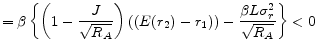(4.1) To show $\frac{dL^{*}}{dE(R_2)} > 0$ , we need to show $\frac{dK}{dE(r_2)} > 0$ .

By linearizing , we have

$\displaystyle K \approx \frac{1}{2\sqrt{R_A}} (2\beta LJ(E(r_2)-r_1)-\beta^{2}L^{2}\sigma_{r}^{2}) + \beta L(E(r_2)-r_1)$

and

$\displaystyle \frac{dK}{dE(r_2)} \approx \frac{\beta LJ}{\sqrt{R_A}} + \beta L + \frac{1}{2}(R_A)^{-\frac{3}{2}} \beta(\beta+1)LJ(2\beta LJ(E(r_2)-r_1)-\beta^{2}L^{2}\sigma_{r}^{2})$

Since

		$\displaystyle \frac{1}{2}(R_A)^{-\frac{3}{2}}\beta(\beta+1)LJ(2\beta LJ(E(r_2)-r_1)-\beta^{2}L^{2}\sigma_{r}^{2})$
		$\displaystyle = \left\{\frac{1}{2}(R_{A})^{-\frac{1}{2}} (2\beta LJ(E(r_2)-r_1) - \beta^{2}L^{2}\sigma_{r}^{2}) \right\} \{(R_A)^{-1}\beta(\beta+1)LJ\}$
		$\displaystyle = -\beta L(E(r_2)-r_1) \{(R_A)^{-1}\beta(\beta+1)LJ\}$

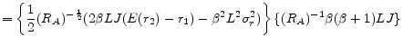the above derivative becomes

$\displaystyle \frac{dK}{dE(r_2)}$		$\displaystyle =\frac{\beta LJ}{\sqrt{R_A}} + \beta L - \beta L (E(r_2)-r_1) \{ (R_A)^{-1}\beta(\beta+1)LJ \}$
		$\displaystyle = \beta L \left[ \frac{J\sqrt{R_A}+\sqrt{R_A}\sqrt{R_A} - (E(r_2)-r_1) \{\beta(\beta+1)LJ\}}{R_A}\right] \nonumber$

Since

$\displaystyle \sqrt{R_A}\sqrt{R_A} \geq J\sqrt{R_A} > \beta LJ(E(r_2)-r_1) \geq \beta^{2}LJ (E(r_2)-r_1)$

we have

$\displaystyle \frac{dK}{dE(r_2)} = \beta L \left[ \frac{J\sqrt{R_A}+\sqrt{R_A}\sqrt{R_A} - (E(r_2)-r_1) \{\beta(\beta+1)LJ\}}{R_A} \right] > 0$

(4.2) To show $\frac{dL^*}{\sigma_{r}^{2}} < 0$ , we need to show $\frac{dK}{d\sigma_{r}^{2}}>0$ .

$\displaystyle \frac{dK}{d\sigma_{r}^{2}} = \frac{d\sqrt{R_A}}{d\sigma_{r}^{2}} = \frac{1}{2} \frac{1}{\sqrt{R_A}} (-\beta^{2}L^{2}) < 0$

(4.3) To show $\frac{dL^*}{dE(P)}>0$ , we need to show $\frac{dK}{dE(P)}>0$ .

$\displaystyle \frac{d\tilde{K}}{dE(P)}$		$\displaystyle = \left(\frac{1}{2}\right)\left(-\frac{1}{2}\right)(R_{A})^{-\frac{3}{2}} (2\beta(J+\beta P_H) - 2\beta^{2}P_L) (2\beta LJ(E(r_2)-r_1) - \beta^{2}L^{2}\sigma_{r}^{2})$
		$\displaystyle = (R_A)^{-\frac{3}{2}} (\beta(J+\beta P_H - \beta P_L)) \{\beta L \sqrt{R_A}(E(r_2)-r_1)\}$
		$\displaystyle =(R_A)^{-1} (\beta(J+\beta P_H - \beta P_L)) \{\beta L (E(r_2)-r_1)\} > 0 \nonumber$

(4.4) To show To show $\frac{dL^{*}}{d\sigma_{r}^{2}}>0$ , we need to show $\frac{dK}{d\sigma_{r}^{2}}<0$ . Since the second period interest rate is uniformly distributed, $\sigma_{r}^{2}=\frac{1}{12}J^2$ , which means $\frac{dK}{d\sigma_{r}^{2}}$ is equivalent to $\frac{dK}{dJ}>0$ .

First, note that

$\displaystyle \frac{dK}{dJ} =$		$\displaystyle \frac{1}{2}\frac{1}{\sqrt{R_F}} \{ 2(J+\beta P_{H})- \beta (2L(1+r_1)+2\beta L(1+E(R_2))) \}$
		$\displaystyle +\frac{1}{2}\frac{1}{\sqrt{R_A}} \{ 2(J+\beta P_{H})- 2\beta L(1+\beta)(1+E(r_2))\}$

Since

$\displaystyle -\frac{(J+\beta P_H)}{\sqrt{R_F}} + \frac{(J+\beta P_H)}{\sqrt{R_A}} = (J+\beta P_H) \left( \frac{\beta L(E(r_2)-r_1)}{\sqrt{R_F}\sqrt{R_A}} \right)$

and

$\displaystyle \frac{\beta L \{ (1+r_{1})+\beta(1+E(r_{2})) \} }{\sqrt{R_{F}}} - \frac{\beta L \{ (1+\beta)(1+E(r_{2})) \} }{\sqrt{R_{A}}}$

$\displaystyle = \beta L \left[ \frac{ \left\{ (1+r_{1})+\beta(1+E(r_{2})) \right\} (\sqrt{R_{F}} - \beta L(E(r_{2})-r_{1})) - (1+\beta) (1+E(r_{2})) \sqrt{R_{F}} }{ \sqrt{R_{F}}\sqrt{R_{A}} } \right]$

$\displaystyle = \beta L \left[ \frac{ -(E(r_{2})-r_{1}) \left\{ \sqrt{R_{F}} + ((1+r_{1})+\beta(1+E(r_{2})))\beta L \right\} }{ \sqrt{R_{F}}\sqrt{R_{A}} } \right]$

we have

$\displaystyle \frac{dK}{dJ} = - \frac{ (J+\beta P_{H}) }{\sqrt{R_{F}}} + \frac{ (J+\beta P_{H}) }{\sqrt{R_{A}}} + \frac{ \beta L \{ (1+r_{1}) + \beta (1+E(r_{2})) \} }{\sqrt{R_{F}}} - \frac{ \beta L (1+\beta)(1+E(r_{2})) }{\sqrt{R_{A}}}$

$\displaystyle =(J+\beta P_{H}) \left( \frac{\beta L(E(r_{2})-r_{1})}{\sqrt{R_{F}}\sqrt{R_{A}}} \right) + \beta L \left[ \frac{ -(E(r_{2})-r_{1}) \{ \sqrt{R_{F}} + ((1+r_{1}) + \beta (1+E(r_{2}))) \beta L \} }{\sqrt{R_{F}}\sqrt{R_{A}}} \right]$

$\displaystyle =\left(\frac{ (J+\beta P_{H})- [ \sqrt{R_{F}} + \{ (1+r_{1})+\beta (1+E(r_{2})) \} \beta L ] }{\sqrt{R_{F}}\sqrt{R_{A}}}\right) \beta L(E(r_{2})-r_{1})$

Recall $J+\beta P_{H} = \sqrt{R_{F}} + \beta L(1+i)$ and $i=r_1+\alpha$ which implies $\left\{ (1+r_{1})+\beta(1+E(r_{2})) \right\} - (1+i) = \beta(1+E(r_{2}))-\alpha > 0$ . Therefore

$\displaystyle \frac{dK}{dJ} = \left( \frac{ (J+\beta P_{H})- [ \sqrt{R_{F}} + \{ (1+r_{1})+\beta (1+E(r_{2})) \} \beta L ] }{\sqrt{R_{F}}\sqrt{R_{A}}} \right) \beta L(E(r_{2})-r_{1}) < 0$

Footnotes

1. Dillon, Shilling, and Sirmans (1987) report that only 8 percent of conventional loans had adjustable rates in early 1981, but that the percentage of adjustable loans steadily increased in the following years, reaching a peak of 65 percent in late 1984. Return to Text

2. Often ARM loans are attractive to borrowers with relatively large financing needs because lower initial interest rates on ARMS produce lower monthly payments than FRMs. ARM borrowers may experience payment difficulties if interest rates rise and income does not rise commensurately with monthly payments. Return to Text

3. Because second mortgages have shorter terms to maturity than first mortgages, second mortgages add disproportionately to the total mortgage debt servicing burden. Return to Text

4. Down payment requirements, which traditionally ranged from 5 to 25 percent of home value, have been extensively studied (Stein (1995), Engelhardt (1996), Ortalo-Magné and Rady (1999, 2000), and Iacoviello( 2005)) and are well understood. Down payments are required by lenders to reduce downside risk at defaults, moral hazard problems in house maintenance, and adverse selection problem due to asymmetric information (Engelhardt (1996)). Households have to build substantial savings themselves or rely on private wealth transfers from a friend or relative to augment savings. Engelhardt and Mayer (1998) report that one in five first time homebuyers receives a financial transfer from a friend or relative to help fund the down payment. These transfers account, on average, for more than half of the down payment amount. Return to Text

5. In an alternative framework where the loan size and the instrument were jointly determined by the borrower, we would first need to consider changes in other variables that may influence choice of loan size. How other exogenous variables cause loan size to change can have very different implications. On the one hand, for example, suppose the loan size changes due to an increase in income. Then the probability of default might stay constant or decrease as the loan size increases. If, on the other hand, loan size changes due to changing riskiness of borrowers, then the probability of default might increase as the loan size increases. These considerations would make the working of the model unnecessarily complicated when our objective is to examine varying effects of loan size on choices of type of interest rate. Return to Text

6. Especially during the later years in the subprime mortgage boom, many subprime lenders were reportedly more accommodating for increasingly larger loans. Return to Text

7. There were many loan programs available for such borrowers during the subprime lending boom. Loan limits up to 125 percent of the house value were common at that time. Ambrose and Sanders (2005) examine effects of state-specific default laws on pricing of such "125 percent LTV" loans. Return to Text

8. For an alternative approach to endogenous LTV, see Ambrose et al (2004). Return to Text

9. For effects of mobility propensity on various ARM product choice, see Fortowsky et al. (forthcoming). Return to Text

10. The empirical measure for the long-term bond risk premium used in this paper and in Koijen, Van Hemert and Van Nieuwerburgh (2009) is the difference between five-year Treasury yield and a three-year average of past one-year Treasury yields. Return to Text

11. Note that divorce rates are measured at the level of state. Compared to other variables measured at the loan level, county level or MSA level, this variable might have been too crudely measured and possibly capture some other unobservable state-wide effects. Return to Text

12. Some contracts have negative fees, i.e., borrowers are credited with upfront cash at the contract to pay initial fees. Borrowers pay for the credit by agreeing to a higher contract rate. Return to Text

13. There is a large literature on trade-off between coupon rate and points in mortgage. See Dunn and Spatt (1988), Chari and Jagannathan (1989), Brueckner (1994) and Stanton and Wallace (1998). Return to Text

^♣ This version is optimized for use by screen readers. Descriptions for all mathematical expressions are provided in LaTex format. A printable pdf version is available. Return to Text