The unreliability of credit-to-GDP ratio gaps in
real-time: Implications for
countercyclical capital buffers*
Keywords: Countercyclical capital buffers, macroprudential policy, Basel III, trend-cycle decomposition, real-time data.
Abstract:
Macroeconomists have long recognized that real-time activity-gap measures are unreliable and that this can present serious difficulties for economic stabilization policies (see Orphanides and Van Norden, 2002, and Staiger, Stock, and Watson, 1997). The use of the nominal credit-to-GDP ratio gap as a reference point for determining the need for accumulating countercyclical capital buffers--as described in the Countercyclical Capital Buffer Proposal of the Basel Committee's Macro Variables Task Force (MVTF)--could potentially suffer from the same problem, thus making it difficult to implement this type of macroprudential policy. This paper follows the approach employed by Orphanides and Van Norden to investigate the relevance of this issue for the U.S. Specifically, we calculate estimates of the credit-to-GDP ratio gap that would have been obtained in real-time and that therefore would have been used in practice in setting countercyclical buffers. We then compare these real-time estimates with ex-post estimates based on all information. Finally, we estimate the potential costs of gap mismeasurement in a practical policy context and find that the volume of lending that could be incorrectly curtailed is large.
As noted by Orphanides and Van Norden there are several reasons why real-time estimates of gap measures can differ from their final estimates. First, the underlying data used to calculate the gap measures can be revised. Second, as data in later periods become available they could alter our estimate of where the trend credit-to-GDP ratio--and therefore the gap--was in earlier periods. Third, incoming data may cause us to revise our model of the time series of the credit-to-GDP ratio that we use to estimate the trend and gap. We consider all three sources of revisions to the U.S. credit-to-GDP ratio gap, although we only consider revisions that arise from the first source (changes to the data) for a limited period of time.1
The MVTF's Consultative Document considers only one method--the Hodrick-Prescott (HP) filter--for extracting the trend credit-to-GDP ratio from the actual ratio. While this is a standard method for trend extraction it is by no means the only one. We therefore consider a range of detrending methods, albeit with the focus on whether they have different revision properties.2
We find that revisions to the U.S. credit-to-GDP ratio gap are sizeable and are on the same order of magnitude as the gap itself. Moreover, the correlation between gaps estimated in real time and gaps estimated based on all available data are low. The main source of the revision is not from revised estimates of the underlying data but rather from the unreliability of end-of-sample estimates of the ratio's trend. Some of the episodes in which we find large revisions to the estimated gap correspond to periods in which the real-time estimate of the gap would have suggested a deployment of countercyclical capital buffers but the final gap would not. We focus on two periods where this was the case, 2001:Q4 and 2003:Q2, and calculate the potential cost of a policy implemented in real time. Using the capital ratios of U.S. banks in the Reports of Conditions and Income, we calculate the change in the system-wide capital shortfall or surplus implied by deploying the capital buffers and derive implications for lending and loan rates. We find that this policy would have acted as an additional drag on the U.S economy following the 2001 recession.
Although the MVTF's Consultative Document does not consider the real-time reliability of gap measures, its analysis is mindful of the distinction between gaps estimated using data available through a particular date and gaps estimated using all available data. For example, the credit-to-GDP ratio gaps reported in the document all extract the one-sided Hodrick-Prescott trend, because this measure only uses information that is available at the time of the observation period.3 That said, the document identifies "protecting the banking sector from periods of excess credit growth" as the objective of countercyclical capital buffers (page 1) and argues that excessive credit growth is well-captured by sizable deviations of the credit-to-GDP ratio above trend (page 18). If we accept that the credit-to-GDP ratio gap provides a good gauge of excess credit growth, then obtaining an accurate measure of the gap is important. Of course, the best estimate of the ratio's trend--and therefore the gap--is obtained from using all available data. But it is exactly this "final" version of the gap that is poorly captured by real-time estimates, according to our analysis.
This paper is organized as follows. Section 1 outlines the detrending methods that we consider and section 2 describes the data that we employ and the "real-time" and "final" trend-estimate concepts that we use. (These concepts--and our taxonomy--are identical to those laid out by Orphanides and Van Norden.) Section 3 reports our results, including our credit-to-GDP ratio gap estimates, the magnitudes of our gap revisions, and some of the effects these revisions can have in real-time and ex post on policy decisions. Section 4 discusses these results while section 5 gauges the potential costs of gap mismeasurement in terms of the volume of lending that could be incorrectly curtailed (or increase in interest rates that could obtain) as a result of basing policy decisions on misleading real-time estimates of the credit-to-GDP ratio gap. Finally, section 6 concludes.
1 Detrending methods
The credit-to-GDP ratio that we consider exhibits distinct upward drift, likely reflecting financial deepening over time. Thus, policymakers would want to consider deviations from the upwardly trending path of the credit-to-GDP ratio in deciding whether to require banks to accumulate countercyclical capital buffers.
We use a number of different detrending methods to estimate the credit-to-GDP ratio gap. All detrending methods separate a series ![]() into a trend component
into a trend component ![]() and a cyclical component
and a cyclical component ![]() ; that is,
; that is,
![]() . Some methods assume that the trend is a deterministic function of time; examples include linear trends, quadratic trends, cubic trends, and cubic splines. Another
method of detrending a series involves applying the HP filter to the series; this is the trend extraction method used in the MVTF's Consultative Document. The final approach that we consider is that of frequency detrending methods. These methods view economic time series as being the weighted
sum of periodic functions (sines and cosines) and consider a series' trend to be that portion of the series that is accounted for by functions that fall within a specified frequency range. We implement this method using an approximate band-pass filter. Our discussion of these various detrending
methods is brief since these methods are well described elsewhere in other sources--see for example Canova (1998) and Orphanides and Van Norden (2002).4
. Some methods assume that the trend is a deterministic function of time; examples include linear trends, quadratic trends, cubic trends, and cubic splines. Another
method of detrending a series involves applying the HP filter to the series; this is the trend extraction method used in the MVTF's Consultative Document. The final approach that we consider is that of frequency detrending methods. These methods view economic time series as being the weighted
sum of periodic functions (sines and cosines) and consider a series' trend to be that portion of the series that is accounted for by functions that fall within a specified frequency range. We implement this method using an approximate band-pass filter. Our discussion of these various detrending
methods is brief since these methods are well described elsewhere in other sources--see for example Canova (1998) and Orphanides and Van Norden (2002).4
1.1 Deterministic detrending methods
Deterministic detrending methods assume that the trend credit-to-GDP ratio can be well approximated by a polynomial function of time, such as a linear, quadratic, or cubic. The trend is the predicted value from a least-squares regression of the credit-to-GDP ratio on a constant and a scaled polynomial function of time; the gap term is the residual from the estimated equation.
If structural change is present, a single deterministic process may not be appropriate for modeling the trend of a series over the entire sample period. We therefore also use a cubic spline detrending procedure in which we divide our sample period into three equal subperiods and fit a separate cubic polynomial over each. At the boundary between two subperiods (called a "knot point"), we restrict the two spline segments to have equal values and equal first and second derivatives (this is essentially a smoothing restriction). Note, our knot points will move when we undertake our real-time analysis.
1.2 The Hodrick-Prescott filter
The HP filter (Hodrick and Prescott, 1980) optimally extracts a smooth stochastic trend that is uncorrelated with the residual cyclical component. Specifically, the trend credit-to-GDP ratio is derived from the HP filter optimization problem:

1.3 Frequency detrending methods
Frequency detrending methods model a time series as a weighted sum of periodic functions (cosines and sines) whose frequencies ranging from 0 to ![]() . Cycles are
fluctuations within a specified range of periodicities or frequencies (where frequency =
. Cycles are
fluctuations within a specified range of periodicities or frequencies (where frequency = ![]() /periodicity).
/periodicity).
As documented by King and Rebelo (1993), the HP filter is an approximation to a frequency-based "high-pass" filter that passes though the higher-frequency fluctuations in a series to the cycle while removing the low-frequency (that is, trend) fluctuations. The HP filter with
![]() approximates a high-pass filter that associates the cyclical component of a series with periodicities that range up to 32 quarters in length (and frequencies that exceed
approximates a high-pass filter that associates the cyclical component of a series with periodicities that range up to 32 quarters in length (and frequencies that exceed
![]() ). Another class of frequency-based filters are "band-pass" filters, which pass through higher-frequency fluctuations, only up to a specified point. That is, certain
high-frequency fluctuations (such as fluctuations that might reflect residual seasonality in the data) are also excluded from the cyclical component along with the low-frequency (trend) components. When we consider band-pass filters, we follow the MVTF's approach of using a range of periodicities
to represent the credit cycle. We first examined periodicities in the band of 6 to 30 quarters (
). Another class of frequency-based filters are "band-pass" filters, which pass through higher-frequency fluctuations, only up to a specified point. That is, certain
high-frequency fluctuations (such as fluctuations that might reflect residual seasonality in the data) are also excluded from the cyclical component along with the low-frequency (trend) components. When we consider band-pass filters, we follow the MVTF's approach of using a range of periodicities
to represent the credit cycle. We first examined periodicities in the band of 6 to 30 quarters (
![]() years), which imply frequencies ranging from
years), which imply frequencies ranging from
![]() to
to
![]() and which result in a credit cycle of about the same length as the business cycle. We also considered periodicities in the band of 6 to 60 quarters ( 15 years), which imply frequencies in the band of
and which result in a credit cycle of about the same length as the business cycle. We also considered periodicities in the band of 6 to 60 quarters ( 15 years), which imply frequencies in the band of
![]() to
to
![]() , and 6 to 90 quarters (
, and 6 to 90 quarters (
![]() years), which imply frequencies in the band of
years), which imply frequencies in the band of
![]() to
to
![]() . These yield credit cycles that are two and three times the length of the business cycle, respectively.
. These yield credit cycles that are two and three times the length of the business cycle, respectively.
An exact band-pass filter cannot be implemented in practice since it requires a two-sided infinite-order moving-average. We use Baxter and King's (1999) finite moving-average approximation, where, following Staiger, Stock, and Watson (2001), we set the width of the two-sided moving-average to 160 quarters to reflect the high degree of persistence in the series we are detrending.
2 Data and real-time/final gap concepts
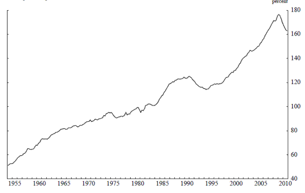
Before reviewing the detrending methods that we use in our study, it is useful to take a look at the series that we are trying to separate into its trend and cycle (gap). The black line in panel A of Figure 1 reports the time series of the nominal credit-to-GDP ratio using the definitions of variables given in the MVTF's Consultative Document and based on 2010:Q4 vintage data. For nominal credit (in the numerator) this is the volume of credit market debt outstanding of the non-financial corporate business sector and household and nonprofit organization sector as reported by the Federal Reserve Board (FRB) in the Flow of Funds Accounts (FOFAs). For nominal GDP (in the denominator) this is the measure reported by the Bureau of Economic Analysis (BEA) in the National Income and Product Accounts (NIPAs).
2.1 Real-time data
Statistical agencies revise data as a result of new source data becoming available over time, re-estimation of seasonal factors, and--most comprehensively--changes in series definitions. These revisions can affect the most recent quarter of the data, the last few years, or the entire history of the series. Revisions to the underlying data used to calculate credit-to-GDP ratios are one reason why gap estimates can change. Studying this source of revision requires that we obtain real-time time series for our nominal credit and nominal GDP series. We obtained our real-time time series for nominal GDP from "ALFRED," which is a data archive maintained by the St Louis Fed. Only a few real-time vintages for nominal credit are available in the ALFRED archive, however. We obtained vintages for these time series from Federal Reserve sources, although past vintages of these time series are only available in electronic form from 1995:Q2.
Although the credit and GDP series are both quarterly, the timing of their releases relative to the data's reference quarter are different. For GDP (and the NIPAs more generally) there are three estimates that are released for a given quarter: the first release, released one month after the reference period; the second release, released two months after; and, the third release, released three months after. After the third release, the data are typically revised only in annual or comprehensive revisions. With credit (and the FOFAs) there is only one release of the data that usually occurs about two-and-a-half months after the reference period. Like the NIPAs there are annual revisions to the FOFAs as well as revisions that occur following NIPAs revisions. In calculating the nominal credit-to-GDP ratio in real time, we use for nominal GDP only the time-series vintages corresponding to the third release; given the different timings of the GDP and credit data releases, this seems to be the most likely value that policymakers would use.
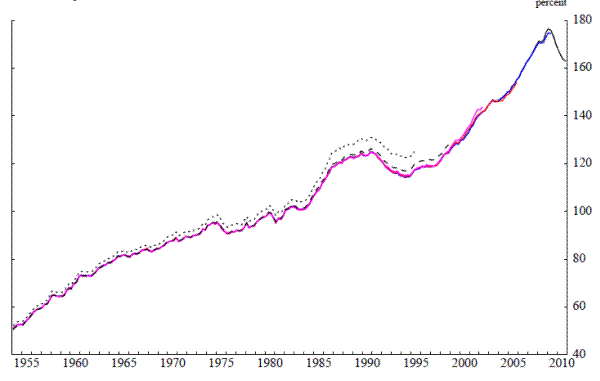
A vintage of data corresponds to the entire time series of the data at a particular point in time. Panel B of Figure 1 plots five vintages of the nominal credit-to-GDP ratio. The name assigned to each vintage corresponds to its last observation. As can seen from panel B, each vintage plotted is different, though the differences are not large. Thus, based on observing the various vintages of the credit-to-GDP ratio one might be inclined to conclude that real-time measurement issues of the credit-to-GDP ratio gap are unlikely to be significant. Our results demonstrate that this is not the case: Real-time measures of the credit-to-GDP ratio gap revise substantially, although--consistent with what is evident from Figure 1--the major source of revision is not revisions to the data.
2.2 Estimates of the nominal credit-to-GDP ratio gap
True real-time estimates: We have sixty-three different vintages of the nominal credit-to-GDP ratio. To obtain the true real-time estimates of the nominal credit-to-GDP ratio gap we first apply our filtering methods (described in section 1) to each of the sixty-three credit-to-GDP ratio vintages, thereby calculating a time series of gaps for each vintage. We then take the last observation of each time series and combine it into a single series.
True final estimates: The true final estimate of the gap uses the full sample of the most recent available vintage of data. For the deterministic trends, the polynomial functions that define the trend are estimated using the most recent vintage of credit-to-GDP ratio data. There are no parameters to be estimated for the HP filter; in this case, the true final estimate of the gap is obtained from the two-sided estimate of the trend. There are also no parameters to be estimated when frequency detrending methods are employed; the true final estimate of the gap here uses--where available--subsequent periods' observations in the moving average calculations that yield the cyclical component of the credit-to-GDP ratio in a given period.
Quasi real-time estimates: As noted in the introduction there are several reasons why the true real-time estimates of the gap should differ from the final estimates; only one of these involves revisions to the data in real time. In order to gauge the role of data revisions alone we calculate quasi real-time estimates of the gap; these are calculated in a similar way to the true real-time gaps but instead of applying our filtering methods to each of our sixty-three time series vintages, we instead apply our filtering methods to the data from our final data vintage, with a rolling endpoint that is set equal to the period for which the gap is being calculated. We then take the last observation of each time series (as we did for the true real-time gap) and combine it into a single series. Thus, the estimate of the gap in any period only uses data up to that point in time, although we use the most recent vintage of data (not the vintage actually available at that time).5
3 Results
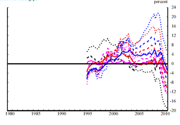
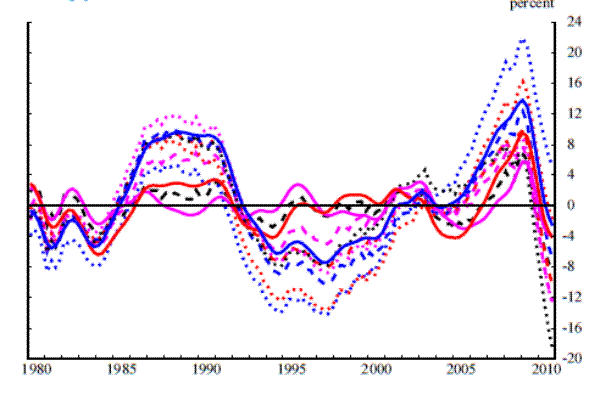
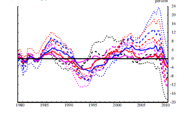
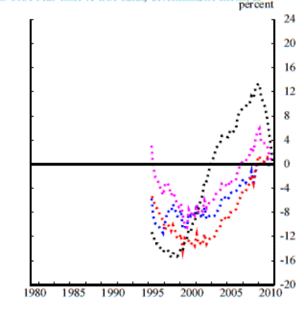
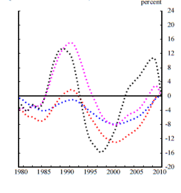
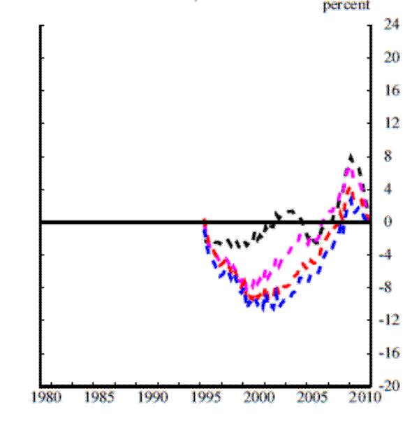
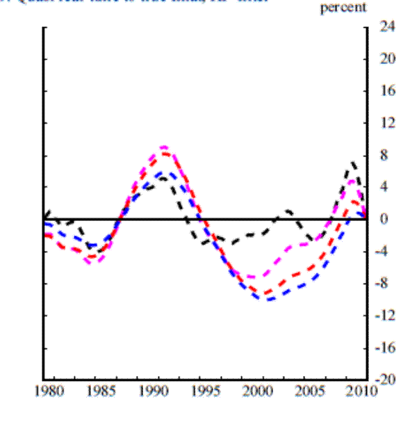
Panel A of Figure 2 plots the true real-time estimates of our credit-to-GDP ratio gap over the period for which we have real-time data, with the gaps measured using all of the detrending methods described in section 1. Panel B (shown below) plots the true final estimates and panel C plots the quasi real-time estimates; for these cases we report results over the 1980:Q1 to 2010:Q4 sample period. With the exception of the cubic spline, the different methods for estimating the trend of the credit-to-GDP ratio yield gaps that display similar contours. The magnitudes of the gaps are quite different, reflecting the fact that for some methods the filter's parameters were set to pass through a greater or lesser share of the credit-to-GDP ratio's fluctuations to the cyclical component.
We begin this section by considering the sources of revision to the real-time credit-to-GDP ratio gap and then examining the magnitudes of the revisions. We then investigate the extent to which revisions could result in different policy actions being taken. After this we examine how quickly revisions tend to be realized, which is a question that could be a concern given that banks have a year in which to build their capital buffers once policymakers call for their deployment. Finally, we discuss how real-time revisions differ across filtering methods.
3.1 Revision sources
The six panels in Figure 3 plot revisions to the credit-to-GDP ratio gap. The three upper panels plot the total revision, that is, the difference between the real-time estimate and the final estimate, while the three lower panels plot the difference between the quasi real-time estimate and the final estimate. Each column in the figure corresponds to a different filtering method.
Comparing the real-time to final and quasi real-time to final revisions reveals that the revisions are fairly similar in terms of both size and contour. Recall that the reason why we constructed the quasi real-time estimate was that revisions to the underlying data represent only one possible source of revisions to estimated gap. Even without revisions to past data, the availability of data for later periods can alter our estimate of where the trend credit-to-GDP ratio was at some earlier point in time and therefore of the gap. Comparing the quasi real-time to final revisions with the true real-time to final revisions allows us to identify the portion of the overall revision that stems from revisions to the data and the portion that stems from the availability of data for later periods. Here, we find that the main source of revisions is not revisions to the underlying data but rather revisions caused by the unreliability of end-of-sample estimates of the trend. This is an important result for understanding why real-time estimates of credit-to-GDP ratio gaps are unreliable, and underscores the fact that different vintages of the credit-to-GDP ratio that do not revise much does not imply that the gap will not revise substantially. This result closely resembles Orphanides and Van Norden's (2002) findings for output-gap estimates.
For the analysis that follows, the result that almost all of the revisions to the credit-to-GDP ratio gap stems from problems with end-of-sample trend estimation (and not from data revisions) means that we can focus on the quasi real-time to final revisions--for which we have a longer sample period--without worrying about missing a sizeable source of revisions. We therefore now consider the quasi real-time to final revisions shown in the lower panels of Figure 3.
3.2 Revision magnitudes
Comparing the lower panels of Figure 3 with the credit-to-GDP ratio gaps shown in Figure 2 indicates that with the exception of the linear trend model (which has extremely large gaps towards the end of the sample) the revision magnitudes are about the same order of magnitude as the gap estimates themselves. This is also evident in Table 1, and the upper panels of Tables 2 and 3, which report key summary statistics for the gap estimates and their revisions.
Table 1 reports the mean, standard deviation, and minimum and maximum values for the final and quasi real-time gaps implied by all of the filtering methods over the period 1980:Q1 to 2010:Q4. (Because the sample period for the data begins 26 years earlier, the means shown in the table need not equal zero.) The upper panel of Table 2 reports similar statistics for the revisions across these gap estimates and for the persistence of these revisions.
The upper panel of Table 3 presents results that assess the reliability of the quasi real-time gap estimates. The first two columns quantify the earlier visual evidence on the magnitudes of the revisions--i.e., the "noise" present in the estimates--relative to the magnitude of the (final) measure itself--i.e., the "signal" from the estimates. The first column reports the ratio of the standard deviation of the revision to the standard deviation of the credit-to-GDP ratio gap, while the second column reports the ratio of the RMSE of the revision to the standard deviation of the credit-to-GDP ratio gap; the difference between these two measures is that the latter reflects any bias that is present in the quasi real-time estimate. (The only notable differences between these two noise-to-signal ratios occur for the gaps implied by linear and quadratic detrending.)
Consistent with the comparison of Figures 2 and 3, the noise-to-signal ratios of the gap estimates are high. The noise measures for the gap estimates in real-time equal 75 percent to 150 percent of the size of the signal for every estimate save those implied by linear and quadratic detrending. (For these measures it is not wholly the case that the standard deviations of the revisions are smaller; much of this result is driven by the range of the gap estimates being so large.)
The remaining columns in the upper half of Table 3 gauge the difference in signal across the quasi real-time and final gap measures. Specifically, the third column reports the correlations between the quasi real-time and final gap measures, and the fourth column reports the fraction of
times that the gap estimates take on different signs. With the exception of the gap implied by the linear trend, the quadratic trend, and to some extent the HP filtered trend with
![]() , the correlations between the quasi real-time and final gaps are relatively low--on the order of 0.35 to 0.7 (this range excludes the cubic spline, for which the correlation is
negative). The number of times that the quasi real-time and final gaps have opposite signs is also quite high--on the order of 25 to 40 percent of the time for most gap estimates. Gap estimates have the opposite sign relatively less frequently for the linear trend (about 10 percent
of the time) but have the opposite sign relatively more frequently for the cubic-spline trend (about two-thirds of the time).
, the correlations between the quasi real-time and final gaps are relatively low--on the order of 0.35 to 0.7 (this range excludes the cubic spline, for which the correlation is
negative). The number of times that the quasi real-time and final gaps have opposite signs is also quite high--on the order of 25 to 40 percent of the time for most gap estimates. Gap estimates have the opposite sign relatively less frequently for the linear trend (about 10 percent
of the time) but have the opposite sign relatively more frequently for the cubic-spline trend (about two-thirds of the time).
3.3 Revisions and ex post policy actions
In using the credit-to-GDP ratio gap to guide policy, an important question is whether the gap accurately signals in real time that policymakers should be requiring banks to accumulate capital buffers. To look at this question we examine whether the quasi real-time and final estimates of the gap typically lie in the upper portions of their respective distributions in identical quarters.
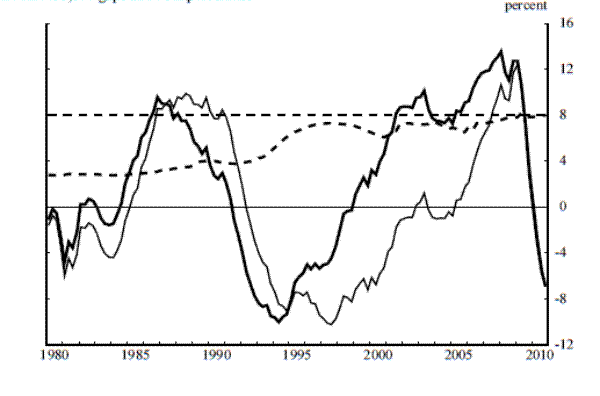
Panel D of Figure 2 shows how we answer this question for the HP filtered trend with ![]() set to 400000. The thick and thin solid black lines shown in panel D are, respectively, the quasi real-time and final gaps implied by this filtering method. The thick dashed black line gives what would have been considered the 90th percentile credit-to-GDP
ratio gap in quasi real-time. We calculate this series iteratively, in the same manner that we calculate the quasi real-time gaps; that is, we extend the sample period-by-period, calculate the gap series and its 90th percentile for that sample, and then combine each 90th percentile
estimate into the single series shown in the figure. (Because the time series of gaps changes with each additional period added to the sample, this 90th percentile series also changes over time.) Finally, the thin dashed line in the figure is the 90th percentile of the final credit-to-GDP
ratio gap; this is the estimate of the 90th percentile of the gap based on all information available up to the end of 2010.
set to 400000. The thick and thin solid black lines shown in panel D are, respectively, the quasi real-time and final gaps implied by this filtering method. The thick dashed black line gives what would have been considered the 90th percentile credit-to-GDP
ratio gap in quasi real-time. We calculate this series iteratively, in the same manner that we calculate the quasi real-time gaps; that is, we extend the sample period-by-period, calculate the gap series and its 90th percentile for that sample, and then combine each 90th percentile
estimate into the single series shown in the figure. (Because the time series of gaps changes with each additional period added to the sample, this 90th percentile series also changes over time.) Finally, the thin dashed line in the figure is the 90th percentile of the final credit-to-GDP
ratio gap; this is the estimate of the 90th percentile of the gap based on all information available up to the end of 2010.
If we take the 90th percentile of the credit-to-GDP ratio gap to be the level at which supervisors would deploy countercyclical capital buffers--which is consistent with the more frequent extreme of the 10- to 20-year incidence described in the MVTF's Consultative Document--we can ask in
which periods countercyclical capital buffers would have been in place in quasi real time.6 For the HP filter with
![]() (panel D of Figure 2), these would be the quarters in which the thick-solid line (representing the gap) exceeds the thick-dashed line (representing the
90th percentile). We can then ask how often for these instances that we also find that the final estimate of the gap exceeds the 90th percentile. The second-to-last column of Table 3 gives this percentage, which in some cases is near zero and never exceeds 40 percent. The last
column of Table 3 then asks for what proportion of the time that the final gap is found to exceed the 90th percentile was the quasi real-time gap also found to be in the 90th percentile. Here we find higher numbers for almost all of the gap measures (except for those generated by the
band-pass filter). This indicates that, for these detrending methods, reacting to levels of credit that appear to be excessive but later turn out not to be is a greater problem than missing--and thereby failing to react when--credit levels are excessive. With the band-pass filter, however, the
opposite is the case.
(panel D of Figure 2), these would be the quarters in which the thick-solid line (representing the gap) exceeds the thick-dashed line (representing the
90th percentile). We can then ask how often for these instances that we also find that the final estimate of the gap exceeds the 90th percentile. The second-to-last column of Table 3 gives this percentage, which in some cases is near zero and never exceeds 40 percent. The last
column of Table 3 then asks for what proportion of the time that the final gap is found to exceed the 90th percentile was the quasi real-time gap also found to be in the 90th percentile. Here we find higher numbers for almost all of the gap measures (except for those generated by the
band-pass filter). This indicates that, for these detrending methods, reacting to levels of credit that appear to be excessive but later turn out not to be is a greater problem than missing--and thereby failing to react when--credit levels are excessive. With the band-pass filter, however, the
opposite is the case.
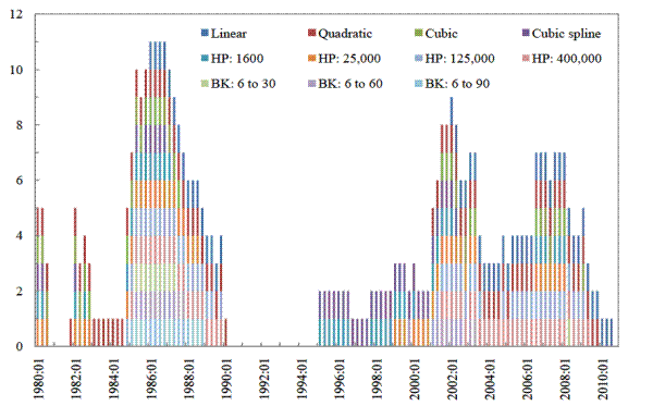
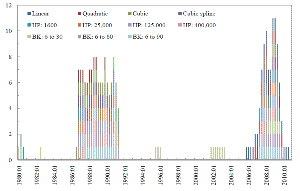
It is evident from Table 3 and panel D of Figure 2 that there are occasions when quasi real-time estimates of the credit-to-GDP ratio gap are very high (specifically, above the quasi real-time estimate of the 90th percentile) even though the final estimates are not excessive by this definition. Figure 4 summarizes the timing of these occasions across all of the filtering methods that we consider. In the upper panel we assign a value of one to all periods in which the quasi real-time gap estimate has a value that puts it above the 90th percentile of the historical distribution of gaps. For each period, we then sum across the different filtering methods that put the quasi real-time gap in the 90th percentile. In the lower panel we do the same thing for the final gap. In the 2001 to 2003 period, many filtering methods indicate that countercyclical capital buffers should have been deployed based on quasi real-time estimates (the upper panel) but not based on full-sample estimates (the lower panel).7We consider in section 5 what the implications these "false positives" might have had for lending. In addition, we would note that for these years the true real-time gap estimate would also have resulted in the deployment of countercyclical capital buffers.
3.4 Within-year revisions
The MVTF's countercyclical capital buffer proposal gives banks one year to accumulate sufficient capital to meet additional regulatory requirements. This raises the concern that if estimates of the credit-to-GDP ratio gap revise substantially within a given year, it may weaken supervisors'
ability to effectively deploy countercyclical capital buffers. The lower panels of Tables 2 and 3 report statistics that address this issue. The first two columns of the lower panel of Table 3 indicate that revisions to the quasi real-time gap over the first year after the estimate
is made are modest for most filtering methods. The exceptions, however, are the HP filter trend with a ![]() value of 1600 and the band-pass filters that allow periodicities of 6 to 30 periods and 6 to 60 periods, for
which two-thirds of the ultimate revision occurs within the first year. (The results of the third and fourth columns are similar.)
value of 1600 and the band-pass filters that allow periodicities of 6 to 30 periods and 6 to 60 periods, for
which two-thirds of the ultimate revision occurs within the first year. (The results of the third and fourth columns are similar.)
The last two columns of this panel consider how the decision to deploy countercyclical capital buffers could change given an extra year of data with which to estimate the gap. As before, we continue to find that false positives are a larger problem for the deterministic detrending methods and the HP filter, while missed responses appear to be a greater concern for the band-pass filter.
4 Revisions and different filtering methods
The relationship between the choice of filtering method and the size and timing of gap-estimate revisions can be summarized as follows. First, the credit-to-GDP ratio gaps obtained from the linear and (to a lesser extent) quadratic detrending methods yield the smallest revisions. Second, deterministic detrending methods with higher-order polynomial trends imply larger revisions while the HP filter and frequency detrending methods that allow for longer credit cycles imply smaller revisions. Finally, gap estimates implied by frequency detrending methods exhibit a larger portion of their revisions quite quickly--that is, within the course of a year--relative to other methods.
The finding that credit-to-GDP ratio gaps implied by linear and quadratic detrending methods have the smallest revisions reflects the problems that other detrending methods have at the endpoints of a series. These problems arise because both unobserved-components and band-pass filtering methods estimate the trend and cycle of a series using past and current values of a series, as well as whatever future observations are available. Toward the end of the sample period fewer future observations are available, which can result in large revisions when data do become available.
The Baxter-King filter, which is implemented as a symmetric two-sided moving average of the actual data uses an estimated AR process to "pad" the sample period with backcasts and forecasts of the series to be filtered. As additional quarters of actual data become available, the future-period
observations and forecasts used in the filter also change, potentially resulting in large revisions to the gap and trend estimates. Of course, the degree to which these estimates of the trend and cycle change depends on the weights in the moving average assigned to the quarters for which new data
and revised forecasts become available. The HP filter, which can also be expressed as a two-sided moving average of the actual data, does not pad the sample period with backcasts and forecasts but instead applies different weights at different points in the sample period. That is, if we are
calculating the cyclical component of a series for the first period of the sample, the coefficients in the moving average applied to the actual data are different from the coefficients applied for the second period in the sample, the third period in the sample, and so on. The amount by which the
moving average coefficients change from one observation to the next depends on where in the sample the observation lies: At the beginning and end of a sample the moving average weights differ greatly from one observation to the next, while in the middle of a large sample the moving average weights
change little. As Baxter and King (1999) discuss, the moving-average weights for an HP filter with
![]() only settle down after about three years.8 This yields significant instability in our real-time estimates of the credit-to-GDP ratio's trend and associated gap measure.
only settle down after about three years.8 This yields significant instability in our real-time estimates of the credit-to-GDP ratio's trend and associated gap measure.
Deterministic detrending methods model the trend as the fitted value of an estimated polynomial function of time, with the cyclical component defined as the residual between the series and the trend. Here, additional quarters of data result in revisions to the trend and the cycle through their effects on the estimated coefficients of the polynomial. In principle, additional quarters of data should alter the trend and cycle only very modestly in large samples because additional observations should yield only slight changes in parameter values. The results in Tables 2 and 3 indicate that this is in fact the case for credit-to-GDP ratio when we use linear or quadratic detrending. However, when we model the trend as a cubic function of time, the real-time reliability of the resulting gap measure is among the poorest of all the filtering methods we consider. This in turn reflects overfitting at the endpoint: As can be seen from the plot of the credit-to-GDP ratio in Figure 1, there is a large run-up and subsequent decline in the series over the early 1980s to early 1990s period. A higher-order polynomial initially attempts to fit this bulge with a small increase in the trend at the end of the sample. As more data become available and the run-up starts to reverse itself, the cubic polynomial calls for a flatter trend, which in turn implies large revisions to the gap. The reason this does not happen for the linear and quadratic trends is that since they never attempt to fit the bulge in the credit-to-GDP ratio; hence their parameter estimates change relatively little around this episode and smaller revisions obtain. This underscores the sensitivity of even relatively low-order polynomial detrending procedures in real-time when the actual series exhibits persistent but ultimately transitory movements.
The cubic spline has the largest revisions of all the methods we consider. This reflects both the problems faced by cubic polynomial detrending, as well as the fact that the estimation intervals for the segments of the spline can be quite small despite a large available time-series of data. Specifically, our time-series of 27 years at the start of our real-time analysis and 57 years over the complete sample translate into spline segments that initially span 9 years of data and eventually span 19 years. Consequently, additional quarters of data can have significant effects on the trend and result in large revisions to the estimated gap.
We would note that although the linear and quadratic trends exhibit the smallest revisions, they are not necessarily the best techniques to use for estimating the credit-to-GDP ratio gap. An augmented Dickey-Fuller test of the credit-to-GDP ratio over the full sample indicates that the series has a unit root and thus has a stochastic trend. This implies that the HP filter and the band-pass filter that are able to remove a unit root are more appropriate to apply to the credit-to-GDP ratio since deterministic detrending methods will generate spurious cycles. Although our focus is on revisions to the various gap estimates, any practical attempt to use a credit-to-GDP ratio gap to guide countercyclical capital policy would require some consideration of issues such as the deterministic or stochastic nature of the trend and the most appropriate filter to use.
Another feature of the estimated revisions implied by the various detrending procedures is that the HP filter and frequency-detrending methods that allow for longer credit cycles imply smaller revisions to the implied gap measures. For the HP filter this arises because longer assumed credit cycles imply a smoother path of the trend (this is associated with a larger penalty on changing the slope of the trend in the HP filter optimization problem--see subsection 1.2). This means that additional observations have a smaller effect on the estimated cyclical component with correspondingly smaller revisions to the gap measure. The intuition for the Baxter-King filter is similar: Allowing for longer credit cycles implies that a smaller range of low-frequency fluctuations are extracted in constructing the cycle; additional observations therefore have smaller effects on the low-frequency component of the series, in turn implying smaller revisions to the cyclical component.
Finally, the result that a larger share of revisions occur within a year if we use filtering methods with shorter credit cycles (e.g., the HP filter trend with a ![]() of 1600 and the bandpass filters that pass through periodicities in of range 6 to 30 quarters) reflects the smaller amounts of data that are needed to change the trend estimates for these filtering methods. Similarly, the different ways
that the HP and band-pass filters deal with end-point problems determines the rapidity with which the bulk of the revisions occur. As noted earlier, it takes about three years before the moving average weights associated with the HP filter settle down; hence, a reasonable fraction of revisions to
the gap occur more than one year after the reference quarter. Revisions to the Baxter-King gaps occur more quickly because the largest moving average weights are on observations that are just a couple of quarters before and after the current observation. Consequently, the largest revisions for the
Baxter-King gaps occur within a year.
of 1600 and the bandpass filters that pass through periodicities in of range 6 to 30 quarters) reflects the smaller amounts of data that are needed to change the trend estimates for these filtering methods. Similarly, the different ways
that the HP and band-pass filters deal with end-point problems determines the rapidity with which the bulk of the revisions occur. As noted earlier, it takes about three years before the moving average weights associated with the HP filter settle down; hence, a reasonable fraction of revisions to
the gap occur more than one year after the reference quarter. Revisions to the Baxter-King gaps occur more quickly because the largest moving average weights are on observations that are just a couple of quarters before and after the current observation. Consequently, the largest revisions for the
Baxter-King gaps occur within a year.
5 Real implications of countercyclical capital buffers
The results of section 3 underscored a key practical difficulty associated with countercyclical capital buffers; specifically, the tendency for credit-to-GDP ratio gaps to yield false positives in terms of indicating excessively high levels of credit in real-time. We now consider the potential real economic costs of deploying countercyclical capital buffers based on unreliable real-time estimates of the credit-to-GDP ratio. We focus on the reduction in lending that would have obtained were countercyclical capital buffers to have been deployed in 2001:Q4 and 2003:Q2, which are the dates for which a number of detrending methods yielded false positives (see section 3.3). The effect of countercyclical capital requirements on lending in these quarters depends on a number of considerations, including the extent to which countercyclical capital requirements would have been binding in these quarters, the capital shortfalls that countercyclical buffers would have implied, and the effect of increased capital requirements on the level of lending and interest rates.
While our paper focuses on the costs of false positives, this should not be read as necessarily implying that countercyclical capital buffers carry no potential benefits. The MVTF's Consultative Document suggests one such benefit, which is that if a credit boom associated with an increase in systemic risk is underway, the deployment of countercyclical capital buffers should leave banks better positioned to absorb losses--which should in turn reduce the risk that regulatory capital requirements will constrain lending when credit-market conditions deteriorate. The document also contends that the build-up of capital buffers carries a possible side benefit in that it might retard the expansion of excess credit. Although the Consultative Document makes no attempt to demonstrate the existence of these benefits (either in the context of a structural model or through past natural experiments), we are broadly sympathetic to these claims on a priori grounds. We focus on the costs of false positives because this addresses the considerations that follow most naturally from our evidence regarding the incidence of false positives in section 3. Moreover, descriptions of the purported potential benefits of countercyclical capital buffers are available elsewhere; see Caruana (2010) for a discussion in the context of the runup to the 2007-2009 crisis.
5.1 Extent that countercyclical capital requirements bind
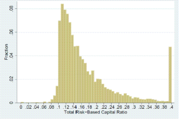
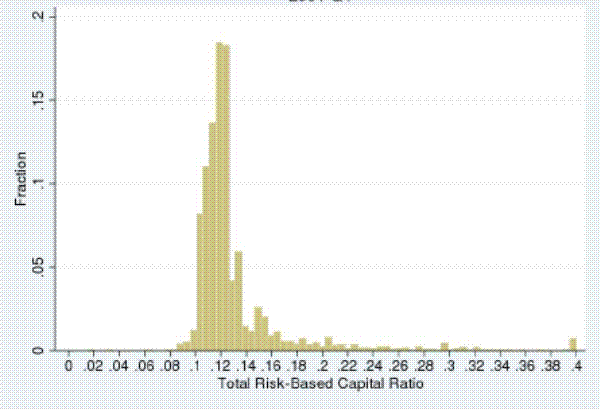
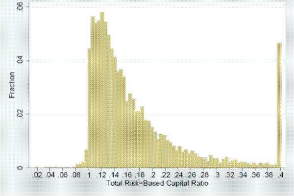
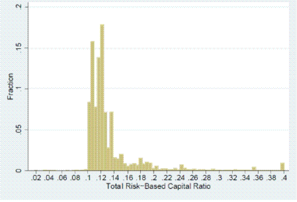
We examine the extent to which countercyclical capital buffers deployed in 2001:Q4 and 2003:Q2 would have been binding by considering the distribution of risk-based capital (RBC) ratios across U.S. banks for these two quarters. The left column of Figure 5 shows the distribution of unweighted RBC ratios in these quarters by institution and the right column shows the distribution of weighted RBC ratios by asset volume. As can be seen from the left column of the figure, in 2001:Q4 and 2003:Q2 nearly all banks met the Federal Deposit Insurance Corporation's (FDIC's) 10 percent total RBC ratio criterion for being well capitalized.9 The right column, however, shows much more bunching in RBC ratios when the ratios are weighted by a bank's total assets, with most of the distribution lying just above the 10 percent cut-off for being well capitalized.
Two observations follow from Figure 5. First, the changes in capital ratio requirements that would have been implied by credit-to-GDP ratio measures in 2001:Q4 and 2003:Q2 would have been binding given that banks strive to keep their capital ratios in the well-capitalized category.10 Second, large banks, who account for the lion's share of assets and capital in the banking sector, have capital ratios that are only slightly above regulatory requirements.11 In sum, these observations imply that changes in capital ratio requirements based on credit-to-GDP ratio measures in 2001:Q4 and 2003:Q2 would have affected a significant share of the economy's bank capital, even if the changes would have affected only a small number of institutions.
5.2 Capital shortfalls implied by countercyclical capital requirements
The data underlying Figure 5 allow us to compute how much capital the banking sector would have needed to raise in 2001:Q4 and 2003:Q2 to meet the capital requirements imposed by countercyclical capital buffers. This calculation is done by determining for each quarter which banks would have had a shortfall of capital relative to the new countercyclical capital buffer requirements, calculating the dollar value of the shortfall for each bank, and summing these individual bank shortfalls together to obtain the aggregate shortfall for the entire banking sector. The upper part of Table 4 shows the outcome of these calculations for a range of countercyclical capital buffer add-ons; specifically, for a 1/2 percentage point, 1 percentage point, 1-1/2 percentage point, and 2 percentage point add-on. (We do not use the maximum possible add-on of 2-1/2 percentage points so as not to obtain extreme results with regard to the potential costs we calculate.)
It is well documented that banks operate with higher capital ratios than are required by regulation, with many factors--including the capital ratio demanded by credit markets, managers' preferences for risk management, and the regulatory and supervisory environment--accounting for the difference between the actual and required capital ratios. (See Alfon, Argimon, and Bascunan-Ambros, 2004.) Thus, we also considered the amount of the capital shortfall in the banking system were banks to hold a precautionary buffer in excess of the higher regulatory minimum. Specifically, we considered the capital shortfall were supervisors to deploy a 2 percentage point countercyclical capital buffer under the assumption that banks want to hold an additional 1/2 percent or 1 percent of capital. (These estimates are also shown in the top panel of Table 4.)
Our calculations suggest the following ranges of estimates for the capital shortfalls that would be implied by countercyclical capital buffers. In 2001:Q4, the total capital shortfall of U.S. banks would have been between $2.1 billion for a capital ratio requirement of 10.5 percent and $58.8 billion for a capital ratio requirement of 12 percent together with a 1 percent precautionary buffer. For 2003:Q2, our estimates are $1.1 billion for a capital ratio requirement of 10.5 percent and $67.3 billion for a capital ratio requirement of 12 percent together with a 1 percent precautionary buffer.
5.3 Impact of capital shortfalls on lending and interest rates
We first address the question of how the capital shortfalls reported in the upper panel of Table 4 would have affected the dollar value of bank lending. There is a wide range of theoretically possible values for the scale of the increase; these range from zero (if banks can costlessly raise equity) to an amount equal to the leverage rate (if banks target regulatory requirements and actively manage their assets). Adopting this latter view, which was quite prominent in the early years of the recent crisis (see Hatzius, 2007 and 2008), would lead to very substantial reductions in assets and loan volumes from a capital shortfall (specifically, we would obtain dollar declines in assets on the order of ten times the dollar value of the capital shortfall). We do not adopt this view because such large effects are odds with what estimated models of bank lending indicate. For example, Hancock and Wilcox (1993, 1994) find that a $1 capital shortfall decreases lending by $1.50; more recently, Berrospide and Edge (2010) estimate the effect of bank capital on lending using bank holding company data and confirm the modest effects of Hancock and Wilcox. In their data, Berrospide and Edge find that a $1 shortfall in bank capital results in a $1.86 reduction in loans.12
The estimates of Berrospide and Edge (2010) reported above focus on bank capital shortfalls in general and not on capital shortfalls following a change in regulatory capital requirements. Hancock and Wilcox (1993) do distinguish capital shortfalls relative to bank-specific targets and relative to regulatory requirements, which arose following the implementation of the Basel Accord. The latter have significantly larger effects on lending, with a $1 regulatory capital shortfall yielding a $3.16 reduction in total lending.
We construct a lower and upper bound for the implications of capital shortfalls implied by countercyclical capital buffers being deployed in 2001:Q4 and 2003:Q2 on lending. The lower bound is the system-wide capital shortfall, excluding any precautionary buffers, multiplied by the $1.86 estimate of Berrospide and Edge for the effect of capital shortfalls on loan volumes.13 The upper bound assumes that banks also build-up a precautionary buffer of one percentage point in excess of the new, higher regulatory minimum. Here we apply different estimates of the effects of capital shortfalls depending on whether the shortfall is a regulatory shortfall or is relative to a banks' own desired capital target: For regulatory shortfalls we apply the Hancock and Wilcox estimate of a $3.16 reduction in loan growth for a $1 capital shortfall, while for for the shortfall relative to the banks' own desired capital ratio we apply the Berrospide and Edge estimate of $1.86.14 The results for all of the capital ratio changes we consider are shown in Table 4. Even without making any extreme assumptions, the effects of countercyclical capital buffers on lending can be substantial. For example, for an additional capital requirement of 2 percentage points, the reduction in lending following 2001:Q4 could have been as much as $141 billion.
Our calculations so far have focused on loan volumes. However, higher capital requirements can also affect banks' funding costs and translate into higher spreads for borrowers. That said, there appears to be little empirical evidence to support this possibility. For example, Meisenzahl (2011) finds no significant effect of funding costs or capital ratios on business loan interest rates in small business loan data. Specifically, for banks with more than $50 billion in assets in the 2003 Survey of Small Business Finances survey sample, Meisenzahl finds that a 10 percentage point increase in the capital ratio increases the business loan interest rate only 23 basis points (this increase is insignificant). Similarly, Hanson, Kashyap, and Stein (2011) report a modest loan interest rate increase of at most 35 basis points for a 10 percentage point increase in the capital ratio.15 In sum, additional countercyclical capital buffers of 1 or 2 percentage points appear unlikely to increase loan interest rates by much.
5.4 Some context for the decline in lending
We now put the reductions in loan volumes reported in Table 4 into context. The range of $3.9 billion to $141.1 billion for 2001:Q4 can be compared for the same time period to new mortgage originations to consumers of about $700 billion and new auto loan originations of about $100 billion, as well as with C&I loan originations of about $88 billion for the first week of November 2001 ($1,114 billion for the quarter). Similarly, the range of $2 billion to $162.1 billion for 2003:Q2 can be compared for the same time period to new mortgage originations of almost $1,000 billion and new auto loan originations of about $75 billion, as well as with C&I loan originations of about $62 billion for the first week of May 2003 ($806 billion for the quarter).16 If we assume that all of the reductions in loan volumes in Table 4 occur in these bank-dependent loan categories (as research by Hancock and Wilcox, 1993, and Peek and Rosengren, 1995, suggests) originations could have been reduced by 7.6 percent and 8.9 percent of total loans in 2001:Q4 and 2003:Q2, respectively.
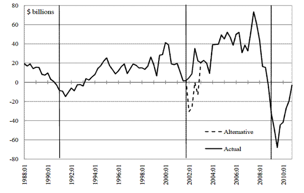
Figure 6 provides a different way of putting the decline in lending reported in Table 4 in context. Here we focus on 2001:Q4, which is also the quarter that the NBER dates as the trough of the 2001 recession. The solid line in panel A of Figure 6 shows the unannualized first difference of the volume of depository institution (DI) loans over the period 1988 to 2010, as reported in the Flow of Funds Accounts. The dotted line subtracts $35.3 billion from the flow of DI loan volumes in each quarter of 2002. This amount equals one-quarter of the $141.1 billion reduction in lending that would have been implied by the deployment of a 2 percentage point countercyclical buffer in 2001:Q4. (We spread the $141.1 billion amount across four quarters because the proposal in the MVTF's Consultative Document gives banks a year to increase their capital ratios.)
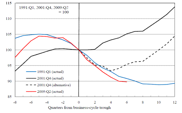
The solid black line in panel B shows the path of real (GDP-price deflated) loan volumes for DIs around 2001:Q4, rescaled to 100 in that quarter. The dashed black line shows the (deflated and rescaled) path of loan volumes around 2001:Q4 assuming the deployment of a 2 percentage point countercyclical capital buffer. As can be seen, the deployment of the buffer would have implied that over the first year following the 2001 recession, real DI loan volumes would have contracted, rather than remaining flat as they did in history.
To see whether such a contraction would have been significant, we overlay on panel B the paths of real DI loan volumes around the NBER troughs of the 1990-91 and 2007-09 recessions (which fell in 1991:Q1 and 2009:Q2, respectively). To make these lines comparable we rescale them so that their values at the trough of each recession are 100. As evident from the figure, had a 2 percentage point capital add-on been put into effect in 2001:Q4 and had banks also chosen to hold an additional 1 percentage point buffer, loan volumes in 2002 would have declined in a manner similar to how they contracted during the credit crunches that followed the 1990-91 and 2007-09 recessions.
To be sure, the MVTF's Consultative Document does not advocate a mechanistic rule in which the buffer is automatically deployed once the indicator variable exceeds some threshold. Rather, the document emphasizes the need for applying "judgment in the setting of the buffer ... using the best information available to gauge the build up of systemic risk" (page 7). Thus, it is unlikely that a buffer would be deployed without policymakers taking other economic conditions into account. Although the use of judgment could reduce the possibility of policymakers imposing countercyclical capital buffers when the economy is in recession, it does not rule it out. Were systemic risks perceived--albeit by a false positive--to have been intensifying in the financial system in late 2001, policymakers could have still deemed it prudent to deploy buffers to ensure that banks would have enough capital to absorb losses once credit conditions deteriorated, even in the face of a downturn.17
6 Conclusions
This paper has assessed the potential cost of the MVTF's proposal to use the credit-to-GDP ratio gap as a reference point for countercyclical capital buffers. Because these gap measures are very unreliable in real time, they provide a poor foundation for policymaking. Specifically, real-time measures of the gap can yield false positives by signalling excessively high levels of credit that later--based on longer time series of data--do not appear to be so extreme. When these measures are used to determine whether countercyclical capital buffers should be deployed, these false positives can in turn result in capital shortfalls in the banking sector and unnecessary lending restraint. We investigate a few instances in which the credit-to-GDP ratio gap does in fact yield a false positive, and find that in these episodes the impact on loan volumes can be highly significant.
To be clear, our paper is not a comprehensive evaluation of all potential costs, benefits, unintended consequences, and regulatory arbitrage possibilities associated with the BCBS's countercyclical capital buffer proposal. In particular, we do not attempt to quantify or provide an analytic demonstration of any of the benefits posited by the MVTF's Consultative Document; rather, our focus is solely on the potential risks of using an unreliable real-time indicator to guide countercyclical capital deployment decisions. Of course, basing decisions on potentially unreliable real-time indicators is a practical complication faced by any type of stabilization policy. But this does not mean that the costs of unreliable real-time indicators should be accepted as an inevitable consequence of policymaking. Rather, what is crucial is to design decisionmaking processes that are robust to the inaccuracies inherent in most real-time indicators and that therefore minimize the attendant costs of using these indicators to inform policy actions. The results of this paper indicate that tying the deployment of countercyclical capital buffers to the credit-to-GDP ratio gap does not meet these criteria.
| Mean | Std. Dev. | Minimum | Maximum | Corr. w/ final | |
| Linear method: Final | -1.08 | 9.09 | -14.20 | 21.95 | |
| Linear method: Quasi real-time | 2.89 | 8.71 | -10.32 | 23.51 | 0.97 |
| Quadratic method: Final | -0.8 | 7.65 | -13.60 | 16.21 | |
| Quadratic method: Quasi real-time | 4.99 | 6.86 | -8.52 | 17.90 | 0.81 |
| Cubic method: Final | 0.46 | 6.27 | -12.97 | 11.89 | |
| Cubic method: Quasi real-time | -0.15 | 6.15 | -13.07 | 8.00 | 0.37 |
| Cubic spline method: Final | 0.10 | 5.90 | -18.74 | 9.46 | |
| Cubic spline method: Quasi real-time | 0.15 | 5.95 | -18.74 | 10.42 | -0.11 |
| HP: 1600 method: Final | -0.01 | 2.30 | -8.47 | 6.98 | |
| HP: 1600 method: Quasi real-time | -0.02 | 2.69 | -9.33 | 3.46 | 0.41 |
| HP: 25000 method: Final | -0.01 | 4.20 | -12.55 | 7.81 | |
| HP: 25000 method: Quasi real-time | 0.92 | 4.74 | -12.55 | 7.75 | 0.45 |
| HP: 125000 method: Final | 0.04 | 5.52 | -10.35 | 9.89 | |
| HP: 125000 method: Quasi real-time | 1.92 | 5.77 | -10.35 | 9.83 | 0.61 |
| HP: 400000 method: Final | -0.10 | 6.35 | -10.21 | 12.39 | |
| HP: 400000 method: Quasi real-time | 2.45 | 6.42 | -9.99 | 13.53 | 0.73 |
| BK: 6 to 30 method: Final | 0.04 | 1.87 | -3.86 | 5.8 | |
| BK: 6 to 30 method: Quasi real-time | 0.07 | 1.14 | -3.86 | 2.27 | 0.56 |
| BK: 6 to 60 method: Final | 0.05 | 3.22 | -6.41 | 9.52 | |
| BK: 6 to 60 method: Quasi real-time | 0.35 | 2.34 | -5.06 | 4.17 | 0.41 |
| BK: 6 to 90 method: Final | 1.03 | 5.93 | -7.41 | 13.8 | |
| BK: 6 to 90 method: Quasi real-time | 1.13 | 3.25 | -5.69 | 5.97 | 0.68 |
| Mean | Std. Dev. | RMSE | Minimum | Maximum | AR | |
| Linear method | -3.97 | 2.38 | 4.63 | -7.96 | 0.00 | 1.000 |
| Quadratic method | -5.79 | 4.49 | 7.32 | -13.03 | 1.79 | 1.002 |
| Cubic method | 0.61 | 6.97 | 6.97 | -8.21 | 15.09 | 0.995 |
| Cubic spline method | -0.05 | 8.84 | 8.80 | -15.85 | 13.34 | 0.994 |
| HP: 1600 method | 0.02 | 2.74 | 2.73 | -4.02 | 7.05 | 0.981 |
| HP: 25000 method | -0.93 | 4.72 | 4.79 | -7.21 | 9.02 | 0.994 |
| HP: 125000 method | -1.87 | 5.01 | 5.33 | -9.14 | 8.19 | 0.997 |
| HP: 400000 method | -2.56 | 4.73 | 5.36 | -10.02 | 5.92 | 0.997 |
| BK: 6 to 30 method | -0.03 | 1.55 | 1.54 | -2.94 | 5.48 | 0.932 |
| BK: 6 to 60 method | -0.30 | 3.11 | 3.11 | -5.85 | 8.76 | 0.970 |
| BK: 6 to 90 method | -0.10 | 4.40 | 4.39 | -6.12 | 9.82 | 0.985 |
| Mean | Std. Dev. | RMSE | Minimum | Maximum | AR | |
| Linear method | -0.20 | 0.75 | 0.78 | -1.60 | 0.99 | 0.989 |
| Quadratic method | -1.02 | 1.35 | 1.69 | -3.04 | 1.76 | 0.992 |
| Cubic method | 0.09 | 2.13 | 2.12 | -2.40 | 4.90 | 0.997 |
| Cubic spline method | -0.33 | 3.44 | 3.44 | -6.33 | 8.86 | 1.022 |
| HP: 1600 method | -0.05 | 1.75 | 1.74 | -2.34 | 6.43 | 1.034 |
| HP: 25000 method | -0.44 | 1.83 | 1.87 | -3.01 | 4.44 | 1.016 |
| HP: 125000 method | -0.59 | 1.59 | 1.69 | -2.63 | 2.73 | 1.000 |
| HP: 400000 method | -0.57 | 1.36 | 1.47 | -2.74 | 2.08 | 0.992 |
| BK: 6 to 30 method | -0.04 | 1.29 | 1.29 | -1.69 | 5.16 | 0.884 |
| BK: 6 to 60 method | -0.05 | 1.87 | 1.86 | -2.56 | 7.70 | 0.882 |
| BK: 6 to 90 method | -0.05 | 2.01 | 2.00 | -2.79 | 8.41 | 0.881 |
| Noise-to-Signal (1) | Noise-to-Signal (2) | Corr. | Opposite Sign | In latter 90 pctl. if in QRT 90 pctl. | In QRT 90 pctl. if in latter 90 pctl. | |
| Linear method | 0.26 | 0.51 | 0.97 | 0.11 | 0.39 | 1.00 |
| Quadratic method | 0.59 | 0.96 | 0.81 | 0.37 | 0.32 | 1.00 |
| Cubic method | 1.11 | 1.11 | 0.37 | 0.39 | 0.21 | 0.30 |
| Cubic spline method | 1.50 | 1.49 | -0.11 | 0.66 | 0.03 | 0.04 |
| HP:1600 method | 1.19 | 1.19 | 0.41 | 0.38 | 0.15 | 0.33 |
| HP:25000 method | 1.12 | 1.14 | 0.45 | 0.40 | 0.19 | 0.39 |
| HP:125000 method | 0.91 | 0.97 | 0.61 | 0.31 | 0.33 | 0.70 |
| HP:400000 method | 0.74 | 0.84 | 0.73 | 0.27 | 0.40 | 0.91 |
| BK:6 to 30 method | 0.83 | 0.82 | 0.56 | 0.30 | 0.10 | 0.05 |
| BK: 6 to 60 method | 0.97 | 0.97 | 0.41 | 0.32 | 0.00 | 0.00 |
| BK: 6 to 90 method | 0.74 | 0.74 | 0.68 | 0.23 | 0.31 | 0.22 |
| Noise-to-Signal (1) | Noise-to-Signal (2) | Corr. | Opposite Sign | In latter 90 pctl. if in QRT 90 pctl. | In QRT 90 pctl. if in latter 90 pctl. | |
| Linear method | 0.08 | 0.09 | 1.00 | 0.01 | 0.92 | 1.00 |
| Quadratic method | 0.18 | 0.22 | 0.99 | 0.03 | 0.88 | 1.00 |
| Cubic method | 0.34 | 0.34 | 0.98 | 0.03 | 0.38 | 1.00 |
| Cubic spline method | 0.58 | 0.58 | 0.87 | 0.17 | 0.05 | 0.67 |
| HP:1600 method | 0.76 | 0.76 | 0.60 | 0.21 | 0.12 | 0.45 |
| HP:25000 method | 0.44 | 0.45 | 0.96 | 0.08 | 0.43 | 0.95 |
| HP:125000 method | 0.29 | 0.31 | 0.99 | 0.03 | 0.46 | 0.96 |
| HP:400000 method | 0.21 | 0.23 | 1.00 | 0.03 | 0.62 | 1.00 |
| BK:6 to 30 method | 0.69 | 0.69 | 0.52 | 0.27 | 0.40 | 0.24 |
| BK: 6 to 60 method | 0.58 | 0.58 | 0.73 | 0.25 | 0.55 | 0.41 |
| BK: 6 to 90 method | 0.34 | 0.34 | 0.85 | 0.12 | 0.75 | 0.48 |
| Capital Shortfall in 2001:Q4 (in billions) | Capital Shortfall in 2003:Q2 (in billions) | Reduction in Lending in 2001:Q4 Lower Bound (in billions) | Reduction in Lending in 2001:Q4 Upper Bound (in billions) | Reduction in Lending in 2003:Q2 Lower Bound (in billions) | Reduction in Lending in 2003:Q2 Upper Bound (in billions) | |
| Required Total Risk-based Capital Ratio: 10.5% | 2.1 | 1.1 | 3.9 | 26.7 | 2.0 | 30.6 |
| Required Total Risk-based Capital Ratio: 11.0% | 5.5 | 6.3 | 10.2 | 52.6 | 11.7 | 61.0 |
| Required Total Risk-based Capital Ratio: 11.5% | 12.9 | 15.7 | 24.0 | 90.9 | 29.2 | 106.7 |
| Required Total Risk-based Capital Ratio: 12.0% | 24.4 | 28.4 | 45.4 | 141.1 | 52.8 | 162.1 |
| Required Total Risk-based Capital Ratio: 12.0% + 0.5% pre-cautionary buffer | 39.9 | 46.4 | ||||
| Required Total Risk-based Capital Ratio: 12.0% + 1.0% pre-cautionary buffer | 58.8 | 67.3 |
Source: Call Reports. The capital shortfall is defined as the total amount of capital need by banks that have capital ratios below the requirements holding assets constant. The lower bound is constructed using the estimates for bank-specific target ratio of $1.86 of lending for $1 of capital as reported in Berrospide and Edge (2010). The upper bound is constructed using the estimates for regulatory capital shortfalls of $3.16 of lending for $1 of capital as reported in Hancock and Wilcox (1993) for each $1 of capital shortfall plus a 1% pre-cautionary bank-specific target buffer with $1.86 of lending for $1 of capital.
Legend for panel A: 10q4 (black, solid).
