
The Effect of Endogenous Human Capital Accumulation on Optimal Taxation
Keywords: Optimal taxation, capital taxation, human capital.
Abstract:
In their seminal works, Chamley (1986) and Judd (1985) determine that it is not optimal to tax capital in an infinitely-lived agent model. In such a model, taxing capital income is equivalent to an ever increasing tax on future consumption, thus implying an exponentially increasing distortion between the marginal rate of substitution and the marginal rate of transformation. In contrast, in a life cycle model agents live for a finite number of periods so the distortion imposed by a capital tax is bounded and may not necessarily be bigger than the distortions caused by other taxes. Atkeson et al. (1999), Erosa and Gervais (2002), and Garriga (2001) demonstrate in simplified life cycle models that if the government cannot condition labor income taxes on age, then it will generally tax capital in order to mimic an age-dependent tax.2 The government wants to condition taxes on age since agents vary their consumption and labor over the life cycle. Quantitative exercises, such as Conesa et al. (2009) and Peterman (2011), demonstrate that in a calibrated life cycle model the inability to condition taxes on age can be a strong motive for a positive tax on capital.
Variation in age-specific human capital causes an agent to vary his labor supply over his lifetime and hence the non-zero tax on capital result.3 Even though age-specific human capital is a driving mechanism for the positive optimal tax on capital, it is typically incorporated in models exogenously through age-specific productivity levels. By including human capital accumulation exogenously, the models ignore any effect that endogenous accumulation may have on the optimal tax policy. This paper assesses, both analytically and quantitatively, the impact of including endogenous age-specific human capital accumulation in a life cycle model on the optimal capital tax.
Specifically, this paper explores the effect on optimal tax policy of including either of two different forms of endogenous age-specific human capital accumulation: learning-by-doing (LBD) and learning-or-doing (LOD). In LBD, an agent acquires human capital by working. In LOD, which is also referred to as Ben Porath type skill accumulation or on-the-job training, an agent acquires human capital by spending time training in periods in which he is also working.4 With LBD, an agent determines his level of age-specific human capital by choosing the hours he works, while with LOD, an agent determines his human capital by choosing the hours he trains. I analyze the effects of both forms, since there is empirical evidence that each form is responsible for age-specific human capital accumulation, and each is commonly employed in quantitative life cycle models.5
Including endogenous human capital accumulation changes the optimal capital income tax. Garriga (2001) demonstrates that in a simplified life cycle model with exogenous age-specific human capital accumulation and a utility function that is both separable and homothetic with respect to consumption and hours worked the optimal tax on capital is zero. In contrast, I analytically demonstrate that including either form of endogenous age-specific human capital accumulation in a similar model causes the optimal tax on capital to be non-zero. Including endogenous human capital accumulation creates an incentive for the government to condition labor income taxes on age. If age-dependent labor income taxes are not in the feasible policy set, then the a non-zero tax on capital is optimal in order to mimic the wedge created by conditioning labor income taxes on age. Specifically, a positive (negative) tax on capital imposes the same wedge on the marginal rate of substitution as a relatively larger (smaller) tax on young labor income. Therefore, including endogenous human capital overturns the zero capital tax result in Garriga (2001).
Furthermore, the form by which one includes endogenous human capital accumulation qualitatively changes the properties of the optimal capital income tax. Adding LBD to the model causes an agent to supply labor relatively less elastically early in his life, which alters the optimal tax policy.6 In a model with exogenous skill accumulation, an agent's only incentive to work is his wage. In a model with LBD, the benefits from working are current wages as well as an increase in future age-specific human capital. I refer to these benefits as the "wage benefit" and the "human capital benefit," respectively. The importance of the human capital benefit decreases as an agent approaches retirement. Thus, adding LBD causes the agent to supply labor relatively less elastically early in his life compared with later in his life. Relying more heavily on a capital tax reduces the distortions that this tax policy imposes on the economy, since it implicitly taxes this less elastically supplied labor income from younger agents at a higher rate than older agents.7 I refer to this channel as the elasticity channel since alterations to the labor supply elasticity profile is responsible for the change in the optimal tax on capital.
Adding LOD to the model also causes a non-zero tax on capital to be optimal if age-dependent taxes are unavailable. There are two channels through which LOD affects the optimal tax policy: the elasticity channel and the savings channel. First, adding LOD changes an agent's elasticity profile. Training is an imperfect substitute for labor as both involve forfeiting leisure in exchange for higher lifetime income. The substitutability of training decreases as an agent ages since he has less time to take advantage of the accumulated skills. Therefore, introducing LOD causes a young agent to supply labor relatively more elastically. The elasticity channel lowers the optimal tax on capital to implicity reduce the relative taxes on labor income of younger agents. The second channel, the savings channel, arises because training is an alternative method of saving, as opposed to accumulating physical capital. Therefore, the government can increase an agent's incentives to train by taxing capital (or taxing young labor income at relatively higher rates) since it makes training a relatively more desirable way to save. Since these two channels have counteracting effects, one cannot analytically determine the cumulative direction of their impact on the optimal tax policy.8
I quantitatively assess the effect of adding each form of endogenous age-specific human capital accumulation on optimal tax policy in a calibrated life cycle model using the specific utility function from Garriga (2001). The optimal tax rates in the model with exogenous age-specific human capital accumulation (exogenous model) are 18.2 percent on capital and 23.7 percent on labor. I find that adding either form of endogenous human capital increases the optimal tax on capital. In the model with LBD the optimal tax rates are 25.5 percent on capital and 22.1 percent on labor. The optimal tax rates in the model with the LOD framework are 18.9 percent on capital and 23.6 percent on labor. Adding endogenous age-specific human capital accumulation raises the optimal tax on capital by approximately forty percent in the LBD framework and approximately four percent in the LOD framework. Overall, the optimal tax on capital is 35 percent higher in the model with LBD compared to the model with LOD indicating that the form by which human capital endogenously accumulates is quantitatively important.
I test the sensitivity of these results with respect to the utility function. I find that using an alternative utility function that is neither separable nor homothetic with respect to consumption and hours worked implies that the optimal tax on capital is much larger in the exogenous model. The optimal tax on capital is larger because with this utility function the Frisch labor supply elasticity profile is upward sloping regardless of the form of human capital accumulation. I find that including either form of endogenous human capital accumulation with this utility function causes an even larger increase in the optimal tax on capital. The optimal tax on capital increases by approximately forty six percent and fifteen percent when LBD and LOD are included, respectively. The optimal tax on capital is approximately twenty seven percent higher in the the LBD model compared to the LOD model. Therefore, even in this set up which has a large motive for a tax on capital in the exogenous model, the form by which human capital endogenously accumulates has large impacts on the optimal capital tax.
Correia (1996), Armenter and Albanesi (2009), and Jones et al. (1997) demonstrate that in a model where the government has an incomplete set of tax instruments a non-zero tax on capital may be optimal in order to mimic the missing taxes. This paper combines two related strands of the literature that examine the optimal tax on capital in such a model where the government does not have a complete set of tax instruments. The first strand examines the optimal tax on capital in a calibrated life cycle model with exogenous human capital where the government cannot condition labor income taxes on age. Conesa et al. (2009), henceforth CKK, solve a calibrated life cycle model to determine the optimal tax on capital. They determine that the optimal tax policy is a flat 34 percent tax on capital and a flat 14 percent tax on labor income.9 They state that a primary motive for imposing a high tax on capital income is to mimic a relatively larger labor income tax on younger agents when they supply labor relatively less elastically. An agent supplies labor more elastically as he ages because his labor supply is decreasing, and the authors use a utility specification in which the agent's Frisch labor supply elasticity is a negative function of hours worked. Peterman (2011) confirms that this is an economically significant motive for the positive tax on capital in a model similar to CKK's model, but concludes that the restriction on the government from being able to tax accidental bequests at a different rate from ordinary capital income is also a large contribution to the positive optimal tax on capital. This paper extends these previous life cycle studies of optimal tax policy by determining the effects of endogenous age-specific human capital accumulation on the optimal tax policy in a standard life cycle model.
This paper is related to a second strand of the literature that analyzes the trade off between labor and capital taxes in a model that includes endogenous age-specific human capital accumulation but not in a life cycle model.10 For example, both Jones et al. (1997) and Judd (1999) examine optimal capital tax in an infinitely lived agent model in which agents are required to use market goods to acquire human capital similar to ordinary capital. They find that if the government can distinguish between pure consumption and human capital investment, then it is not optimal to distort either human or physical capital accumulation in the long run. Reis (2007) shows in a similar model that if the government cannot distinguish between consumption and human capital investment, then the optimal tax on capital is still zero as long as the level of capital does not influence the relative productivity of human capital. Chen et al. (2010) find in an infinitely lived agent model with labor search, that including endogenous human capital accumulation through both LBD and LOD causes the optimal tax on capital to increase because a higher tax on capital unravels the labor market frictions. The labor market frictions causes lower employment in the economy. In Chen et al. (2010), a tax on capital causes the wage discount to increase, thus causing firms to post more vacancies which in turn causes an increase in worker participation. This paper is related to this second strand of literature, however it differs in that it analyzes optimal tax policy in an overlapping generations (OLG) model as opposed to an infinitely lived agent model. Therefore, the second strand of literature does not account for the effects of endogenous human capital accumulation through life cycle channels. It is especially important to include the life cycle channel since Conesa et al. (2009) and Peterman (2011) demonstrate that this channel is quantitatively important for motivating a positive tax on capital. This paper combines both strands of the literature and determines the optimal tax policy in a life cycle model with endogenously determined human capital.
This paper is organized as follows: Section 2 examines an analytically tractable version of the model to demonstrate that including endogenous human capital accumulation creates a motive for the government to condition labor income taxes on age. Section 3 describes the full model and the competitive equilibrium used in the quantitative exercises. The calibration and functional forms are discussed in section 4. Section 5 describes the computational experiment, and section 6 presents the results. Section 7 tests the sensitivity of the results with respect to calibration parameters and utility specifications, while section 8 concludes.
1 Analytical Model
In this section, I demonstrate that adding endogenous human capital accumulation overturns the result from Garriga (2001) that for a specific utility function that is separable and homothetic in both consumption and labor the government has no incentive to condition labor
income taxes on age. I begin this section by setting up the agent's problem and demonstrating that a positive (negative) tax on capital induces a wedge on the marginal rate of substitution that is similar to a relatively larger tax on young (old) labor income. Using the primal approach, I then
solve for the optimal tax policy in the exogenous model, with a benchmark utility function that is homothetic with respect to consumption and hours worked,
 . I confirm the Garriga (2001) result that the government
has no incentive to condition labor income taxes on age and therefore the optimal tax on capital is zero. I show that adding endogenous human capital accumulation to this model causes the optimal tax policy to include age-dependent taxes and if age-dependent taxes are unavailable, then a non-zero
tax on capital is optimal. I also demonstrate the channels by which the forms of endogenous human capital accumulation affect the optimal tax policy.
. I confirm the Garriga (2001) result that the government
has no incentive to condition labor income taxes on age and therefore the optimal tax on capital is zero. I show that adding endogenous human capital accumulation to this model causes the optimal tax policy to include age-dependent taxes and if age-dependent taxes are unavailable, then a non-zero
tax on capital is optimal. I also demonstrate the channels by which the forms of endogenous human capital accumulation affect the optimal tax policy.
I derive these analytical results in a tractable two-period version of the computational model. For tractability purposes, the features I abstract from include: retirement, population growth, progressive tax policy, and conditional survivability. Additionally, I assume that the marginal products of capital and labor are constant. This assumption permits me to focus on the life cycle elements of the model, in that changes to the tax system do not affect the pre-tax wage or rate of return. Since the factor prices do not vary, I suppress their time subscripts in this section. All of these assumptions are relaxed in the computational model.
1.1.1 General Set-up
In the analytically tractable model, agents live with certainty for two periods, and their preferences over consumption and labor are represented by
where
and
where
The agent's problem is to maximize equation 1 subject to 4. The agent's first order conditions are
and
where
1.1.2 Tax on Capital Mimics Age-Dependent Tax on Labor
To demonstrate why a tax on capital has a similar effect to an age-dependent labor income tax, I derive the intertemporal Euler equation by combining equations 5, 6, and 7:
Equation 8 demonstrates that if the government wants to create a wedge on the marginal rate of substitution by varying the age-dependent labor income taxes, then
1.1.3 Primal Approach
I use the primal approach to determine the optimal tax policy.14 I use a social welfare function that maximizes utility and discounts future generations
with social discount factor ![]() ,
,
![\displaystyle [U(c_{2,0},h_{2,0})/\theta]+\sum_{t=0}^{\infty}\theta^{t}[U(c_{1,t},h_{1,t})+\beta U(c_{2,t+1},1-h_{2,t+1})].](img33.gif) |
(9) |
The government maximizes this objective function with respect to two constraints: the implementability constraint and the resource constraint.15 The implementability constraint is the agent's intertemporal budget constraint, with prices and taxes replaced by his first order conditions (equations 5, 6, and 7)
| (10) |
Including this constraint ensures that any allocation the government chooses can be supported by a competitive equilibrium. The resource constraint is
Including the benchmark utility specification, the Lagrangian the government maximizes is
 |
(12) | |
 |
where
1.1.4 Optimal Tax Policy
I solve for the optimal tax policy in the analytically tractable exogenous model. The formulation of the government's problem and their first order conditions for this model can be found in appendix 8.1. Combining the government's first order conditions generates the following expression for optimal labor income taxes:
Equation 13 demonstrates that the government has no incentive to condition labor income taxes on age when age-specific human capital is exogenous.16
Utilizing the first order condition from the Lagrangian with respect to capital and consumption leads to the following equation:
Applying the benchmark utility function to equation 7 provides the following relationship:
Equations 14 and 15 demonstrate that in order for the household to choose the optimal allocation indicated by the primal approach, the tax on capital must equal zero.17
1.2.1 Including LBD Creates Motive for Age-Dependent Taxes on Labor Income
Next, I introduce LBD into the exogenous model. In the LBD model, age-specific human capital for a young agent is normalized to unity. Age-specific human capital for an old agent is determined by the function
![]() . The function
. The function
![]() is a positive and concave function of the hours worked when young. In this model agents maximize the same utility function subject to
is a positive and concave function of the hours worked when young. In this model agents maximize the same utility function subject to
| (17) |
and
| (18) |
The agent's first order conditions are given by
![\displaystyle \frac{U_{h1}(t)}{U_{c1}(t)}=-[w(1-\tau_{h,1})+\beta\frac{U_{c2}(t+1)}{U_{c1}(t)}w (1-\tau_{h,2})h_{2,t+1}s_{h1}(t+1))],](img49.gif)
and
The first order conditions with respect to
 |
(22) |
where
The formulation for the government's problem and the resulting first order conditions (utilizing the benchmark utility function) are in appendix 8.2. Combining the first order conditions from the government's problem and suppressing the time arguments yields the following ratio for optimal labor income taxes,
![\begin{displaymath}\begin{split}\frac{1-\tau_{h,1}}{1-\tau_{h,2}}&= \\ & \frac{\big[1+h_{2,t+1}s_{h2}\big]\big[1+\lambda_{t}(1+\frac{h_{1,t}s_{h2}}{s_{2}})(1+\frac{1}{\sigma_{2}})\big]} {1+\lambda_{t}(1+\frac{1}{\sigma_{2}})-\beta h_{2,t+1}^{1+\frac{1}{\sigma_{2}}}h_{1,t}^{-\frac{1}{\sigma_{2}}} \Bigg[\frac{s_{h2}}{s_{2}}(1+\lambda_{t}(1+\frac{h_{1,t}s_{h2}}{s_{2}}))(1+\frac{1}{\sigma_{2}}) - h_{1} \Big( \big(\frac{s_{h2}}{s_{2}}\big)^{2}-\frac{s_{h2,h2}}{s_{2}}\Big) \Bigg]} \\ & -\frac{h_{2,t+1}s_{h2}}{1+r(1-\tau_{k})}. \end{split}\end{displaymath}](img57.gif)
Equation 23 demonstrates that generally in the LBD model the government has an incentive to condition labor income taxes on age. This result contrasts with the exogenous model, in which the government has no incentive to condition labor income taxes on age (see equation 13).
1.2.2 LBD Enhances Motive for Postive Tax on Capital
I solve for the intertemporal Euler equation (by combining equations 19, 20 and 21) to demonstrate why including LBD causes the optimal tax policy to include age-dependent taxes and which agents the government wants to tax at a higher rate,:
Comparing equation 8 and equation 24, it is clear that the LBD intertemporal Euler equation has an extra term that is positive. Therefore, holding all else equal, the tax on young labor income must be relatively higher to induce the same wedge on the marginal rate of substitution in the LBD model.18 If age-dependent taxes are not in the governments feasible set, then a larger tax on capital will be necessary to induce the same wedge.
By examining the Frisch elasticities in the exogenous and LBD models, it is clear why adding LBD increases the optimal relative tax on young labor income or tax on capital. Since the functional forms of these elasticities extend to a model where agents live for more than two periods, I denote an
agent's age with ![]() . In the exogenous model, the Frisch elasticity simplifies to
. In the exogenous model, the Frisch elasticity simplifies to
![]() . The Frisch elasticity in the LBD model is,
. The Frisch elasticity in the LBD model is,
 . 19
. 19
The Frisch elasticity in the exogenous model is constant and valued at
![]() . In the LBD model, the extra terms in
. In the LBD model, the extra terms in
![]() increase the size of the denominator, thus holding hours and consumption constant between the two models,
increase the size of the denominator, thus holding hours and consumption constant between the two models,
![]() . Intuitively, the inclusion of the human capital benefit makes workers less responsive to a one-period change in wages since the wage benefit is only
part of their total compensation for working in the LBD model. However, the human capital benefit does not have a constant effect on an agent's Frisch elasticity over his lifetime. The relative importance of the human capital benefit decreases over an agent's lifetime because he has fewer periods
to use his higher human capital as he ages.20 Therefore, adding LBD causes a young agent to supply labor relatively less elastically than an older agent.
This shift in relative elasticities creates an incentive for the government to tax the labor income of younger agents at a relatively higher rate. Thus, if the government cannot condition labor income taxes on age, then the optimal tax on capital is higher in the LBD model. I use the
term"elasticity channel" to describe the effect on optimal tax policy caused by a change in the Frisch elasticity from including endogenous human capital. The elasticity channel is responsible for the change in optimal tax policy from including LBD.
. Intuitively, the inclusion of the human capital benefit makes workers less responsive to a one-period change in wages since the wage benefit is only
part of their total compensation for working in the LBD model. However, the human capital benefit does not have a constant effect on an agent's Frisch elasticity over his lifetime. The relative importance of the human capital benefit decreases over an agent's lifetime because he has fewer periods
to use his higher human capital as he ages.20 Therefore, adding LBD causes a young agent to supply labor relatively less elastically than an older agent.
This shift in relative elasticities creates an incentive for the government to tax the labor income of younger agents at a relatively higher rate. Thus, if the government cannot condition labor income taxes on age, then the optimal tax on capital is higher in the LBD model. I use the
term"elasticity channel" to describe the effect on optimal tax policy caused by a change in the Frisch elasticity from including endogenous human capital. The elasticity channel is responsible for the change in optimal tax policy from including LBD.
1.3.1 Including LOD Creates Motive for Age-Dependent Taxes on Labor Income
I include LOD in the exogenous model to demonstrate that this form of endogenous age-specific human capital accumulation also creates a motive for the government to condition labor income taxes on age. Similar to the other models, age-specific human capital for a young agent is set to unity.
Age-specific human capital for an old agent is determined by the function
![]() which is a positive and concave function of the hours spent training when an agent is young (
which is a positive and concave function of the hours spent training when an agent is young (![]() ). In the LOD model I need a utility function that incorporates training. I alter the benchmark utility specification so that it consistently incorporates the disutility to non-leisure activities,
). In the LOD model I need a utility function that incorporates training. I alter the benchmark utility specification so that it consistently incorporates the disutility to non-leisure activities,
 . In this model agents maximize their utility function subject to
| (25) |
and
| (26) |
The agent's first order conditions are given by
![\displaystyle \frac{U_{h1}(t)}{U_{c1}(t)}=-[w(1-\tau_{h,1})],](img71.gif)
and
The first order conditions with respect to
The formulation of the government's problem and resulting first order conditions are provided in appendix 8.3. Combing the first order conditions yields the following relationship for optimal taxes on labor income:
Equation 31 demonstrates that the government has an incentive to condition labor income taxes on age when LOD is introduced into the model.
Although equation 31 shows that including LOD creates an incentive for the government to condition labor income taxes on age, it is unclear at which age the government wants to impose a relatively higher labor income tax. Comparing equations 13 and 31, there are two channels through which introducing LOD changes the optimal tax policy. The first channel results from using a utility function that is non separable in training and labor. The non separability affects the optimal tax policy
through the elasticity channel since it causes LOD to alter the Frisch elasticity. This channel causes the numerator of the ratio to include the additional term
![]() . As a result of this new term, the expression decreases.
. As a result of this new term, the expression decreases.
The second channel results from the intertemporal link created by the additional constraints. I refer to this channel as the savings channel because this model has an additional intertemporal link since agents can save via training. This second channel causes the inclusion of the additional
terms
![]() and
and
![]() in the denominator and numerator, respectively.22 Assuming that
in the denominator and numerator, respectively.22 Assuming that ![]() is positive, these additional terms cause the expression to increase.23 Thus, the two channels have opposing effects on the optimal tax policy, and the overall effect is unclear.24
is positive, these additional terms cause the expression to increase.23 Thus, the two channels have opposing effects on the optimal tax policy, and the overall effect is unclear.24
Examining the Frisch labor supply elasticities provides intuition for how the first channel affects the optimal tax policy. In the exogenous model, the Frisch elasticity for the benchmark utility specification is constant,
![]() . Since the altered utility function is not additively separable in time spent working and training, the Frisch labor supply elasticity is not constant in the LOD model. The Frisch
elasticity for the altered utility function is
. Since the altered utility function is not additively separable in time spent working and training, the Frisch labor supply elasticity is not constant in the LOD model. The Frisch
elasticity for the altered utility function is
![]() . This functional form implies that an agent supplies labor relatively more elastically when LOD is included in the model because the agent has a
substitute for working in the form of training. Additionally, the effect on the Frisch elasticity is larger when he spends a larger proportion of his non-leisure time training (or when training is a better substitute for for generating lifetime income). Therefore, if an agent spends less time
training as he ages, then he will supply labor relatively more elastically when he is young, and the government would want to tax the labor income from young agents at a relatively lower rate. One way to mimic this age-dependent tax is to decrease the tax on capital. Therefore, the elasticity
channel from LOD causes a decrease in the optimal tax on capital.
. This functional form implies that an agent supplies labor relatively more elastically when LOD is included in the model because the agent has a
substitute for working in the form of training. Additionally, the effect on the Frisch elasticity is larger when he spends a larger proportion of his non-leisure time training (or when training is a better substitute for for generating lifetime income). Therefore, if an agent spends less time
training as he ages, then he will supply labor relatively more elastically when he is young, and the government would want to tax the labor income from young agents at a relatively lower rate. One way to mimic this age-dependent tax is to decrease the tax on capital. Therefore, the elasticity
channel from LOD causes a decrease in the optimal tax on capital.
Examining an agent's first order condition with respect to training demonstrates how the savings channel affects the optimal tax policy. An agent optimizes his choices such that the marginal disutility of training when he is young equals marginal benefit of training (
![]() ). The marginal benefit is reduced by decreasing the tax on capital or by increasing the tax on older labor
income. By adopting either of these changes, the government makes it relatively more beneficial for the agent to use ordinary capital to save as opposed to training. Therefore, the government decreases the tax on capital to promote a larger ordinary capital stock.
). The marginal benefit is reduced by decreasing the tax on capital or by increasing the tax on older labor
income. By adopting either of these changes, the government makes it relatively more beneficial for the agent to use ordinary capital to save as opposed to training. Therefore, the government decreases the tax on capital to promote a larger ordinary capital stock.
Overall, adding LOD creates an incentive for the government to condition labor income taxes on age. If the government cannot condition labor income taxes on age, then it would want to implement a non-zero tax on capital to mimic an age-dependent tax. The tax on capital increases when LBD is added to the model. Adding LOD causes the optimal tax on capital to change, however the direction of the change is not analytically clear.
2 Computational Model
To determine the direction and magnitude of the effect of adding endogenous human capital accumulation on optimal tax policy, I solve for the optimal tax policies in the LBD and LOD models and compare them with the exogenous model. The exogenous model is adapted from CKK; however I use a different benchmark utility function so that the elasticity channel does not effect the optimal tax policy in the exogenous model. Additionally, since the authors find that neither idiosyncratic earnings risk nor heterogenous ability types are important motives for a positive tax on capital income, I exclude these sources of heterogeneity. In this section I describe the models and define the competitive equilibrium for each model.
2.1 Demographics
In the computational model, time is assumed to be discrete, and there are J overlapping generations. Conditional on being alive at age ![]() ,
, ![]() is the probability of an agent living to age
is the probability of an agent living to age ![]() . All agents who live to an age of
. All agents who live to an age of ![]() die in the next period. If an agent dies with assets, the assets are confiscated by the government and distributed equally to all the living agents as transfers (
die in the next period. If an agent dies with assets, the assets are confiscated by the government and distributed equally to all the living agents as transfers (![]() ). All agents are required to retire at an exogenously set age
). All agents are required to retire at an exogenously set age ![]() .
.
In each period a cohort of new agents is born. The size of the cohort born in each period grows at rate ![]() . Given a constant population growth rate and conditional survival probabilities,
the time invariant cohort shares,
. Given a constant population growth rate and conditional survival probabilities,
the time invariant cohort shares,
![]() , are given by
, are given by
 for for |
(32) |
where
 |
(33) |
2.2 Individual
An individual is endowed with one unit of productive time per period that he divides between leisure and non-leisure activities. In the exogenous and LBD models the non-leisure activity is providing labor. In the LOD model the non-leisure activities include training and providing labor services to the market. An agent chooses consumption as well as how to spend his time endowment in order to maximize his lifetime utility
 |
(34) |
where
In the exogenous model an agent's age-specific human capital is
![]() . In the endogenous models, an agent's age-specific human capital,
. In the endogenous models, an agent's age-specific human capital, ![]() , is endogenously determined. In the LBD model
, is endogenously determined. In the LBD model ![]() is a function of a skill accumulation parameter, previous age-specific human capital, and time worked, denoted by
is a function of a skill accumulation parameter, previous age-specific human capital, and time worked, denoted by
![]() . In the LOD model,
. In the LOD model, ![]() is
a function of a skill accumulation parameter, previous age-specific human capital, and time spent training, denoted by
is
a function of a skill accumulation parameter, previous age-specific human capital, and time spent training, denoted by
![]() .
.
![]() is a sequence of calibration parameters that are set so that in the endogenous models, under the baseline-fitted U.S. tax policy, the agent's choices result in
an agent having the same age-specific human capital as in the exogenous model. Individuals command a labor income of
is a sequence of calibration parameters that are set so that in the endogenous models, under the baseline-fitted U.S. tax policy, the agent's choices result in
an agent having the same age-specific human capital as in the exogenous model. Individuals command a labor income of
![]() in the exogenous model and
in the exogenous model and
![]() in the endogenous model. Agents split their labor income between consumption and savings with a risk-free asset. An agent's level of assets is denoted
in the endogenous model. Agents split their labor income between consumption and savings with a risk-free asset. An agent's level of assets is denoted ![]() , and the asset pays a pre-tax net return of
, and the asset pays a pre-tax net return of ![]() .
.
2.3 Firm
Firms are perfectly competitive with constant returns to scale production technology. Aggregate technology is represented by a Cobb-Douglas production function. The aggregate resource constraint is,
| (35) |
where
2.4 Government Policy
The government has two fiscal instruments to finance its consumption, ![]() , which is in an unproductive sector.25 First, the government taxes capital income,
, which is in an unproductive sector.25 First, the government taxes capital income,
![]() , according to a capital income tax schedule
, according to a capital income tax schedule
![]() . Second, the government taxes each individual's taxable labor income. Part of the pre-tax labor income is accounted for by the employer's contributions to social security, which
is not taxable under current U.S. tax law. Therefore, the taxable labor income is
. Second, the government taxes each individual's taxable labor income. Part of the pre-tax labor income is accounted for by the employer's contributions to social security, which
is not taxable under current U.S. tax law. Therefore, the taxable labor income is
![]() , which is taxed according to a labor income tax schedule
, which is taxed according to a labor income tax schedule
![]() . I impose three restrictions on the labor and capital income tax policies. First, I assume human capital is unobservable, meaning that the government cannot tax human capital
accumulation. Second, I assume the rates cannot be age-dependent. Third, both of the taxes are solely functions of the individual's relevant taxable income in the current period.
. I impose three restrictions on the labor and capital income tax policies. First, I assume human capital is unobservable, meaning that the government cannot tax human capital
accumulation. Second, I assume the rates cannot be age-dependent. Third, both of the taxes are solely functions of the individual's relevant taxable income in the current period.
In addition to raising resource for consumption in the unproductive sector, the government runs a pay-as-you-go (PAYGO) social security system. I include a simplified social security program in the model because Peterman (2011) demonstrates that excluding this type of
program in a model with exogenously determined retirement causes unrealistic life cycle profiles. In this reduced-form social security program, the government pays ![]() to all individuals
that are retired. Social security benefits are determined such that retired agents receive an exogenously set fraction,
to all individuals
that are retired. Social security benefits are determined such that retired agents receive an exogenously set fraction, ![]() , of the average income of all working individuals. An agent's
social security benefits are independent of his personal earnings history. Social security is financed by taxing labor income at a flat rate,
, of the average income of all working individuals. An agent's
social security benefits are independent of his personal earnings history. Social security is financed by taxing labor income at a flat rate,
![]() . The payroll tax rate
. The payroll tax rate
![]() is set to assure that the social security system has a balanced budget each period. The social security system is not considered part of the tax policy that the government
optimizes.
is set to assure that the social security system has a balanced budget each period. The social security system is not considered part of the tax policy that the government
optimizes.
2.5 Definition of Stationary Competitive Equilibrium
In this section I define the competitive equilibrium for the exogenous model. See appendix 9 for the definition of the competitive equilibriums in the endogenous models.
Given a social security replacement rate ![]() , a sequence of exogenous age-specific human capital
, a sequence of exogenous age-specific human capital
![]() , government expenditures
, government expenditures ![]() , and a sequence of
population shares
, and a sequence of
population shares
![]() , a stationary competitive equilibrium in the exogenous model consists of the following: a sequence of agent allocations,
, a stationary competitive equilibrium in the exogenous model consists of the following: a sequence of agent allocations,
![]() , a production plan for the firm
, a production plan for the firm ![]() , a
government labor tax function
, a
government labor tax function
![]() , a government capital tax function
, a government capital tax function
![]() , a social security tax rate
, a social security tax rate ![]() , a utility function
, a utility function
![]() , social security benefits
, social security benefits ![]() , prices
, prices ![]() , and transfers
, and transfers ![]() such that:
such that:
- Given prices, policies, transfers, and benefits, the agent maximizes the following:
 Max
Max![\displaystyle _{c_{j},h_{j},a_{j+1}}\beta^{j-1}[\prod_{q=0}^{j-1}\Psi_{q}]u(c_{j},h_{j})](img137.gif)
(36)
subject to![\displaystyle c_{j}+a_{j+1}=w\epsilon_{j}h_{j}-\tau_{ss}w\epsilon_{j}h_{j},+(1+r)(a_{j}+Tr)-T^{l}[w\epsilon_{j}h_{j}(1-.5\tau_{ss})] -T^{k}[r(a_{j}+Tr)],](img138.gif)
(37)
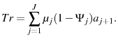
for , and
, and
![\displaystyle c_{j}+a_{j+1}=SS+(1+r)(a_{j}+Tr)-T^{k}[r(a_{j}+Tr)],](img140.gif)
(38)
for . Additionally,
(39)
and
(40) - Prices
 and
and  satisfy
(41)
and
(42) - The social security policies satisfy
(43)
and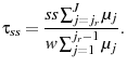
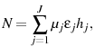
(44) - Transfers are given by
(45) - Government balances its budget
![\displaystyle G=\sum_{j=1}^{J}\mu_{j} T^{k}[r(a_{j}+Tr)] + \sum_{j=1}^{j_{r}-1} \mu_{j}T^{l}[w\epsilon_{j}h_{j}(1-.5\tau_{ss})].](img149.gif)
(46) - The market clears

(47)
(48)
and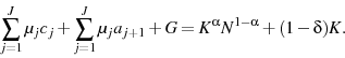
(49)
3 Calibration and Functional Forms
To determine the optimal tax policy it is necessary to choose functional forms and calibrate the model's parameters. Calibrating the models involves a two-step process. The first step is choosing parameter values for which there are direct estimates in the data. These parameter values are in table 1. Second, to calibrate the remaining parameters, values are chosen so that under the baseline-fitted U.S. tax policy certain targets in the model match the values observed in the U.S. economy.26 These values are in table 2
| Value | Target | |
| Demographics Parameter: Retire Age: |
65 | By Assumption |
| Demographics Parameter: Max Age: |
100 | By Assumption |
| Demographics Parameter: Surv. Prob: |
Bell and Miller (2002) | Data |
| Demographics Parameter: Pop. Growth: |
1.1% | Data |
| Firm Parameters: |
.36 | Data |
|---|---|---|
| Firm Parameters: |
8.33% |
|
| Firm Parameters: A | 1 | Normalization |
Adding endogenous human capital accumulation to the model fundamentally changes the model. Accordingly, if the calibration parameters are the same, then the value of the targets will be different in the endogenous and exogenous models. To assure that all the models match the targets under the baseline-fitted U.S. tax policy, I calibrate the set of parameters based on targets separately in the three models. This calibration implies that these parameters are different in the exogenous and endogenous models.
3.1 Demographics
In the model, agents are born at a real world age of 20 that corresponds to a model age of 1. Agents are exogenously forced to retire at a real world age of 65. If an individual survives until the age of 100, he dies the next period. I set the conditional survival probabilities in accordance with the estimates in Bell and Miller (2002). I assume a population growth rate of 1.1 percent.
| Exog. | LBD | LOD | Target | |
| Calibration Parameter: Conditional Discount: |
0.995 | 0.993 | 0.997 | |
| Calibration Parameter: Unconditional Discount:
|
0.982 | 0.980 | 0.984 | |
| Calibration Parameter: Risk aversion:
|
2 | 2 | 2 | CKK |
| Calibration Parameter: Frisch Elasticity:
|
0.5 | 0.73 | 0.47 | Frisch
|
| Calibration Parameter: Disutility to Labor: |
61 | 46 | 80 | Avg.
|
| Government Parameter:
|
.258 | .258 | .258 | Gouveia and Strauss (1994) |
|---|---|---|---|---|
| Government Parameter:
|
.768 | .768 | .768 | Gouveia and Strauss (1994) |
| Government Parameter: G | 0.137 | 0.136 | 0.13 | 17% of Y |
| Government Parameter: b | 0.5 | 0.5 | 0.5 | CKK |
3.2 Preferences
Agents have time-separable preferences over consumption and labor services, and conditional on survival, they discount their future utility by ![]() . I use the benchmark utility function
for the exogenous and LBD models,
. I use the benchmark utility function
for the exogenous and LBD models,
 , and an altered form of this utility function for the LOD model,
.
, and an altered form of this utility function for the LOD model,
.
I determine ![]() such that the capital-to-output ratio matches U.S. data of 2.7.27 I determine
such that the capital-to-output ratio matches U.S. data of 2.7.27 I determine ![]() such
that under the baseline-fitted U.S. tax policy, agents spend on average one third of their time endowment in non-leisure activities.28 Following CKK, I set
such
that under the baseline-fitted U.S. tax policy, agents spend on average one third of their time endowment in non-leisure activities.28 Following CKK, I set
![]() , which controls the relative risk aversion.29 Past micro-econometric studies estimate the Frisch elasticity to be between 0 and 0.5.30 However, more recent research has shown that these estimates may be biased downward. Reasons for this bias include: utilizing weak instruments; not accounting for borrowing constraints;
disregarding the life cycle effect of endogenous-age specific human capital; omitting correlated variables such as wage uncertainty; and not accounting for labor market frictions.31 Furthermore, Rogerson and Wallenius (2009) show that because individuals make decisions regarding labor on both the intensive and extensive margins "micro and macro elasticities need not be the same, and ... macro elasticities can be
significantly larger."32 Therefore, I set
, which controls the relative risk aversion.29 Past micro-econometric studies estimate the Frisch elasticity to be between 0 and 0.5.30 However, more recent research has shown that these estimates may be biased downward. Reasons for this bias include: utilizing weak instruments; not accounting for borrowing constraints;
disregarding the life cycle effect of endogenous-age specific human capital; omitting correlated variables such as wage uncertainty; and not accounting for labor market frictions.31 Furthermore, Rogerson and Wallenius (2009) show that because individuals make decisions regarding labor on both the intensive and extensive margins "micro and macro elasticities need not be the same, and ... macro elasticities can be
significantly larger."32 Therefore, I set
![]() such that the Frisch elasticity is at the upper bound of the range ( 0.5). The preference parameters are summarized in table 2.
such that the Frisch elasticity is at the upper bound of the range ( 0.5). The preference parameters are summarized in table 2.
3.3 Age-Specific Human Capital
The age-specific human capital parameters that require calibration are different in the exogenous and endogenous models. In the exogenous model, I set
![]() so that the sequence matches a smoothed version of the relative hourly earnings estimated by age in Hansen (1993). In the LBD model,
agents accumulate age-specific human capital according to the following process,
so that the sequence matches a smoothed version of the relative hourly earnings estimated by age in Hansen (1993). In the LBD model,
agents accumulate age-specific human capital according to the following process,
| (50) |
where
| (51) |
where
To calibrate the rest of the LBD parameters, I rely on the estimates in Chang et al. (2002), setting
![]() and
and
![]() . Following Hansen and Imrohoroglu (2009), I set
. Following Hansen and Imrohoroglu (2009), I set
![]() and
and
![]() in the LOD model. The value of
in the LOD model. The value of
![]() implies that there is little depreciation of human capital when skill accumulation is the result of LOD.34 The values of
implies that there is little depreciation of human capital when skill accumulation is the result of LOD.34 The values of
![]() and
and
![]() imply that at the start of an agent's career the ratio of time spent training to working is approximately 10 percent and declines steadily until retirement. Through the agent's entire working life, the ratio of the average time spent training to market hours is about 6.25 percent. This average value is in line with the calibration target in Hansen and Imrohoroglu (2009).35
imply that at the start of an agent's career the ratio of time spent training to working is approximately 10 percent and declines steadily until retirement. Through the agent's entire working life, the ratio of the average time spent training to market hours is about 6.25 percent. This average value is in line with the calibration target in Hansen and Imrohoroglu (2009).35
3.4 Firm
I assume the aggregate production function is Cobb-Douglas. The capital share parameter, ![]() , is set at .36. The depreciation rate is set to target the observed investment output ratio of 25.5 percent. These parameters are summarized in table 1.
, is set at .36. The depreciation rate is set to target the observed investment output ratio of 25.5 percent. These parameters are summarized in table 1.
3.5 Government Policies and Tax Functions
To calibrate parameters based on the targets, it is necessary to use a baseline tax function that mimics the U.S. tax code so that I can find the parameter values that imply the targets in the models that match the values in the data. I use the estimates of the U.S. tax code in Gouveia and Strauss (1994) for this tax policy, which I refer to as the baseline-fitted U.S. tax policy. The authors match the U.S. tax code to the data using a three parameter functional form,
where
In addition to government consumption, the government also runs a balanced-budget social security program. Social security benefits are set so that the replacement rate, ![]() , is
50 percent.37 The payroll tax,
, is
50 percent.37 The payroll tax, ![]() , is determined so that the social security system is balanced each period.
, is determined so that the social security system is balanced each period.
4 Computational Experiment
The computational experiment is designed to determine the tax policy that maximizes a given social welfare function. I choose a social welfare function (SWF) that corresponds to a Rawlsian veil of ignorance (Rawls (1971)). Since living agents face no earnings uncertainty, the social welfare is equivalent to maximizing the expected lifetime utility of a newborn,
![\displaystyle SWF(\tau_{h}, \tau_{k})=\sum_{j=1}^{J}\beta^{j-1}[\prod_{q=0}^{j-1}\Psi_{q}]u(c_{j},h_{j}),](img193.gif) |
(53) |
where
To determine the effects of endogenous human capital accumulation, I compare the tax policies that maximize the SWF in the three models. When I determine the optimal tax policy, I test different values of ![]() and determine values for
and determine values for ![]() so that the changes in the tax policy are revenue neutral. Therefore, the experiment is to find
so that the changes in the tax policy are revenue neutral. Therefore, the experiment is to find ![]() that satisfies
that satisfies
| (54) |
subject to,
![\displaystyle G=\sum_{j=1}^{J}\mu_{j} \tau_{k}r(a_{j}+Tr)] + \sum_{j=1}^{j_{r}-1} \mu_{j}\tau_{h}[ws_{j}h_{j}(1-.5\tau_{ss})].](img196.gif) |
(55) |
5 Results
In this section I quantitatively assess the effects on the optimal tax policy of including endogenous age-specific human capital accumulation in a life cycle model. I determine the optimal tax policies in the exogenous, LBD, and LOD models and then highlight the channels that cause the differences. To fully understand the effects of endogenous human capital accumulation, I analyze the aggregate economic variables and life cycle profiles in all three models. I compare the aggregate economic variables and life cycle profiles in all three models under the baseline-fitted U.S. tax policy as well as the changes induced by implementing the optimal tax policies in each specific model.
5.1 Optimal Tax Policies in Exogenous, LBD, and LOD Models
Table 3 describes the optimal tax policies in the three models. The optimal tax policy in the exogenous model is an 18.2 percent flat tax on capital income (
![]() and a 23.7 percent flat tax on labor income (
and a 23.7 percent flat tax on labor income (
![]() .39 While the optimal tax on
capital is smaller in the exogenous model compared with CKK, it is not zero. The motives that cause a positive tax on capital in the exogenous model include: the inability of the government to borrow; agents being liquidity constrained, and the government not being able to tax transfers at a
separate rate from ordinary capital income. See Peterman (2011) for a thorough discussion of the relative strengths of these motives in a model similar to the exogenous model.
.39 While the optimal tax on
capital is smaller in the exogenous model compared with CKK, it is not zero. The motives that cause a positive tax on capital in the exogenous model include: the inability of the government to borrow; agents being liquidity constrained, and the government not being able to tax transfers at a
separate rate from ordinary capital income. See Peterman (2011) for a thorough discussion of the relative strengths of these motives in a model similar to the exogenous model.
The optimal tax policy in the LBD model is
![]() and
and
![]() , and in the LOD model it is
, and in the LOD model it is
![]() and
and
![]() . The optimal tax on capital is approximately forty percent larger in the LBD model and four percent larger in the LOD compared to the exogenous model.
. The optimal tax on capital is approximately forty percent larger in the LBD model and four percent larger in the LOD compared to the exogenous model.
| Tax Rate | Exog | LBD | LOD |
| 18.2% | 25.5% | 18.9% | |
| 23.7% | 22.1% | 23.6% | |
|
|
0.77 | 1.16 | 0.8 |
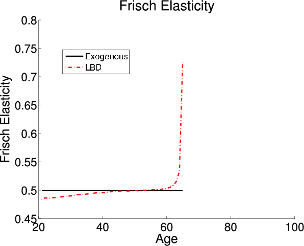
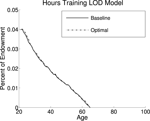
With respect to LBD, the alteration in the Frisch labor supply elasticity profile is the principal reason that the optimal tax on capital increases. The left panel of figure 1 plots the lifetime Frisch labor supply elasticities in the LBD model and the exogenous model under the optimal tax policy. The lifetime labor supply elasticity is flat in the exogenous model and upward sloping in the LBD model. Adding LBD causes agents to supply labor relatively more elastically as they age because the human capital benefit decreases. The optimal tax on capital is higher in the LBD model in order to implicitly tax younger agents, who supply labor less elastically, at a higher rate.
To quantify the effect of the elasticity channel on the optimal tax policy in the LBD model, I alter the exogenous model so that the shape of the lifetime Frisch labor supply elasticity profile is the same as it is in the LBD model under the optimal tax policy. In order to match the shapes of
the profiles, I vary
![]() in the exogenous model by age. I find that the optimal tax policy in this altered exogenous model,
in the exogenous model by age. I find that the optimal tax policy in this altered exogenous model,
![]() and
and
![]() , is almost identical to the optimal tax policy in the LBD model. The optimal tax policy in the altered exogenous model demonstrates that the elasticity channel is responsible
for the change in the optimal tax on capital in the LBD model.40
, is almost identical to the optimal tax policy in the LBD model. The optimal tax policy in the altered exogenous model demonstrates that the elasticity channel is responsible
for the change in the optimal tax on capital in the LBD model.40
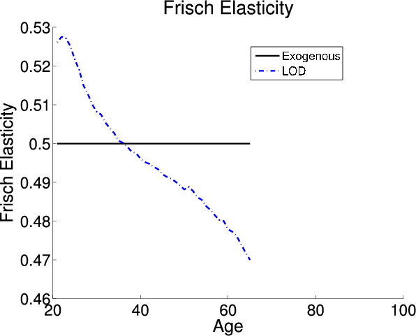
In section 1.3.1 I show that both the elasticity channel and the savings channel affect the optimal tax on capital in the LOD model. Adding LOD to the model causes young agents to supply labor relatively more elastically. The right panel of figure 1 plots the Frisch elasticity profile in the exogenous and LOD models. The elasticity channel causes a decrease in the optimal tax on capital so that younger agents who supply labor more elastically are implicitly taxed at a lower rate. Additionally, the inclusion of LOD allows individuals to use training to save, which activates the savings channel. Analytically, one can not determine the directions of the saving channel's effect of the effect on optimal tax policy.
To quantify the direction of the saving channel's effect and significance of both channels, I solve for the optimal tax policy in an alternative version of the LOD model that excludes the effect from the elasticity channel. I utilize an alternative utility function,
 , which is
separable in training and hours worked. Since the utility function is separable, the Frisch labor supply elasticity is no longer a function of the time spent training. The Frisch elasticity with this utility function is constant, at the value
, which is
separable in training and hours worked. Since the utility function is separable, the Frisch labor supply elasticity is no longer a function of the time spent training. The Frisch elasticity with this utility function is constant, at the value
![]() , so the elasticity channel is eliminated.41 The optimal tax policy in this model with the alternative utility function is
, so the elasticity channel is eliminated.41 The optimal tax policy in this model with the alternative utility function is
![]() and
and
![]() . These results indicate that in this model, the savings channel results in an increase in the optimal tax on capital of 1.7 percentage points, which encourages agents to save via physical capital as opposed to human capital. I find that that the elasticity channel causes the optimal tax on capital to decrease 1 percentage point cancelling just over half of the savings channel's effect.
. These results indicate that in this model, the savings channel results in an increase in the optimal tax on capital of 1.7 percentage points, which encourages agents to save via physical capital as opposed to human capital. I find that that the elasticity channel causes the optimal tax on capital to decrease 1 percentage point cancelling just over half of the savings channel's effect.
5.2 The Effects of Adding Endogenous Age-Specific Human Capital
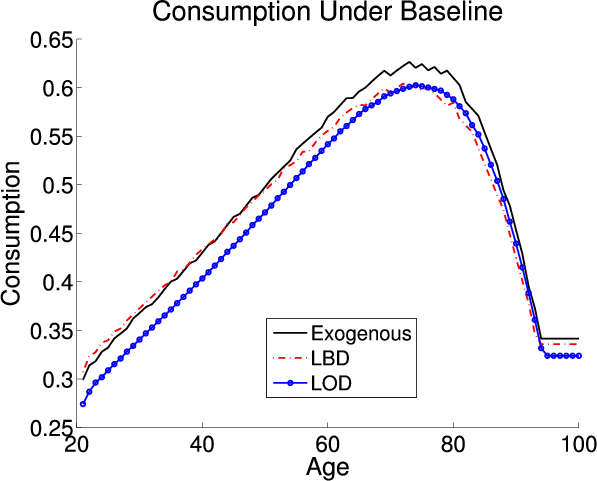
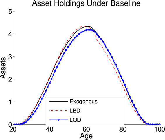
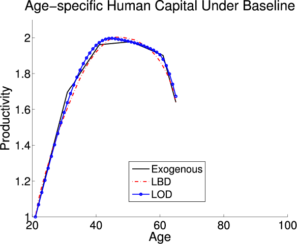
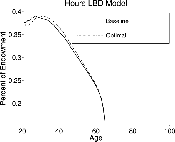
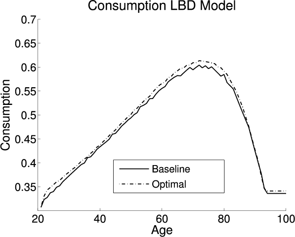
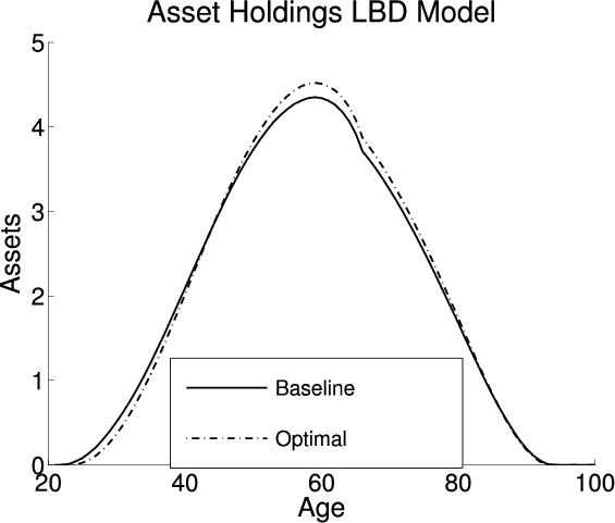
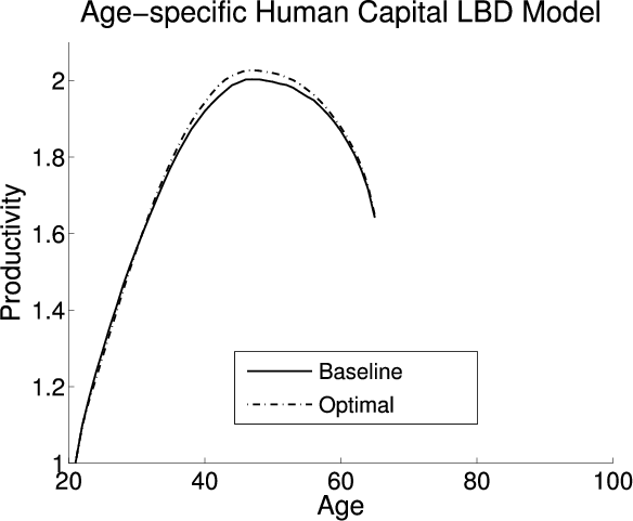
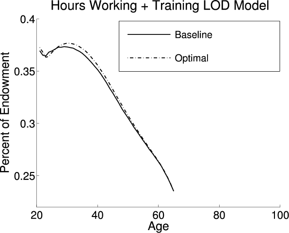
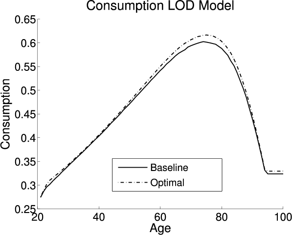
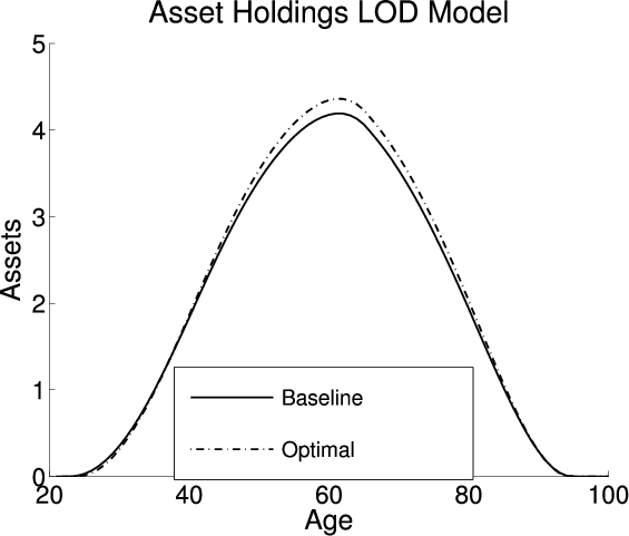
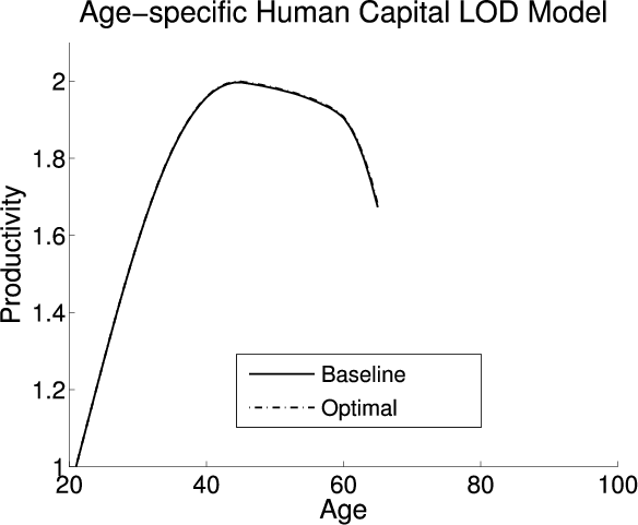
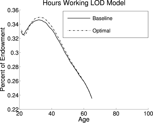
This section analyzes the effect on the aggregate economic variables and life cycle profiles from adding LBD and LOD to the exogenous model under the baseline-fitted U.S. tax policy. Figure 2 plots the life cycle profiles of hours, consumption, assets, and age-specific human capital in all three models. Table 4 describes the optimal tax policies and summarizes the aggregate economic variables under both the baseline-fitted U.S. tax policy and optimal tax policies. The first, fourth, and seventh columns are the aggregate economic variables under the baseline-fitted U.S. tax policy in the exogenous, LBD, and LOD models, respectively. The second, fifth, and eighth columns are the aggregate economic variables under the optimal tax policies. The third, sixth, and ninth columns are the percentage changes in the aggregate economic variables induced from adopting the optimal tax policies.
Note: The average hours refers to the average percent of time endowment worked in the productive labor sector. Both the marginal and average tax rates vary with income under the baseline-fitted U.S. tax policy. The marginal tax rates are the population weighted average marginal tax rates for each agent.
Comparing the first and fourth columns of table 4, it is clear that the levels of aggregate hours, labor supply, and aggregate capital are similar in the exogenous and LBD models. The calibrated parameters are determined so that under the baseline-fitted U.S. tax policy the models match certain targets from the data. Since many of the aggregate economic variables are targets and these calibration parameters are determined separately in the exogenous and LBD models, the aggregates are similar in the two models.
|
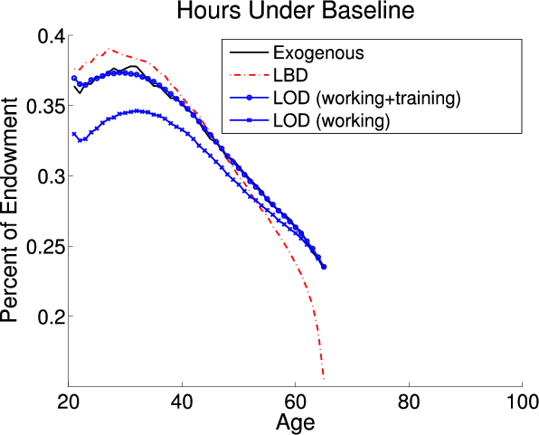
Although adding LBD does not have a large effect on the aggregate economic variables, it does cause changes in the life cycle profiles. Adding LBD causes agents to work relatively more at the beginning of their working life when the human capital benefit is larger, and less later when the benefit is smaller (see the solid black and dashed red lines in the upper-left panel of figure 2).
The upper-right panel shows that the lifetime consumption profile is steeper in the exogenous model. The intertemporal Euler equation controls the slope of consumption profile over an agent's lifetime. The relationship is
where
Although the parameters values are calibrated such that the targets still match, the size of the economy is smaller in the LOD model because agents must spend time training in this model. Comparing the first and seventh columns of table 4, aggregate labor supply, and physical capital are smaller in the LOD model compared with the exogenous model because an agent spends part of his time endowment training. However, it is apparent that the relative ratios of the aggregates are similar in the two models since the factor prices are comparable.
Adding LOD also affects the life cycle profiles. Figure 2 plots two labor supply profiles for the LOD model -- the first is solely hours spent working, and the second is the sum of hours spent working and training (see the blue lines in the upper-left panel). The LOD labor supply profile that includes training is similar to the labor supply profile in the exogenous model; however the profile that excludes training is smaller. The difference between the two LOD profiles is the amount of time spent training. This gap shrinks as an agent ages, representing a decrease in the amount of time spent training. Agents spend less time training as they age because the benefits decrease since they have fewer periods to take advantage of their human capital. Adding LOD causes the size of the economy to decrease causing a shift down in the life cycle profile for consumption. In the LOD model, agents can use their time endowment to accumulate human capital, which acts as an alternative form of savings from assets. Therefore, during their working lives, agents hold less ordinary capital and opt to use human capital to supplement their savings. As an agent approaches retirement the value of the human capital decreases and the ordinary savings profile in the LOD model converges to the profile in the exogenous model. Finally, similar to LBD, the lifetime age-specific human capital profiles are similar in the exogenous and LOD models since the profiles are a calibration target.
5.3 The Effects of the Optimal Tax Policy in the Exogenous Model
This section examines the effects on the economy of adopting the optimal tax policy in the exogenous model. In the exogenous model, the optimal tax on capital is smaller than the average marginal tax under the baseline-fitted U.S. tax policy so adopting the optimal tax policy causes an increase in aggregate capital (see columns one and two of figure 4). The average marginal tax on labor is also less under the optimal tax policy than the baseline so the labor supply increases.42 The increase in labor supply is relatively less than the increase in capital so the rental rate on capital decreases and the wage rate increases.
To compare the welfare effects of adopting the optimal tax policies in the models, I compute the consumption equivalent variation (CEV). The CEV is the uniform percentage increase in consumption, at each age, needed to make an agent indifferent between being born under the baseline-fitted U.S. tax policy and the optimal tax policy. Therefore, a positive CEV indicates a welfare increase due to tax reform. Overall, adopting the optimal tax policy in the exogenous model causes a welfare increase of 0.7 percent CEV.43
|
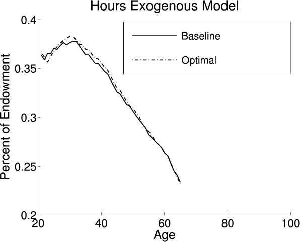
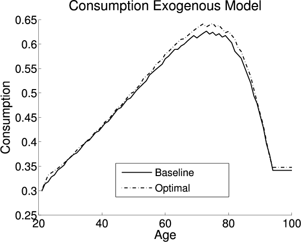
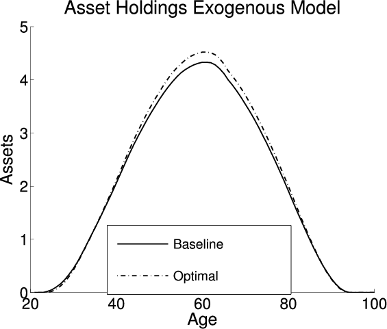
Figure 3 plots the life cycle profiles for time worked, consumption, assets and age-specific human capital in the exogenous model under the baseline-fitted U.S. tax policies and the optimal tax policies. The solid lines are the profiles under the baseline-fitted U.S. tax policies, and the dashed lines are the profiles under the optimal tax policies. Adopting the optimal tax policy in the exogenous model causes changes in all three life cycle profiles: (i) early in their life, agents work relatively more; (ii) agents save more, especially during periods when they are wealthier; and (iii) the lifetime consumption profile steepens. Comparing the profiles in the left panel of figure 3, it is evident that agents work more early in their life because of the lower implicit tax on young labor income due to a decrease in the tax rate on capital income.
Implementing the optimal tax policy causes a decrease in both the tax on capital and the rental rate on capital. These changes have competing effects on the marginal after-tax return on capital that are not consistent for all individuals. Specifically, since the baseline fitted US tax on capital is progressive and the optimal tax is flat, the change in the tax rate has an uneven effect on an agent's net return over his lifetime. The decrease is larger for agents who hold more savings since their marginal tax rate was higher under the progressive baseline fitted US tax policy. Overall, the after tax return increases for middle-aged agents and decreases for younger and older agents when the optimal tax policy is adopted. In response to these changes, middle-aged individuals increase there savings under the optimal tax policy. In contrast, younger and older agents decrease their savings (see the lower left panel of figure 3).
Similar to savings, the slope of an agents consumption profile is controlled by the marginal after-tax return to capital (see equation 56). Therefore, adopting the optimal tax policy causes a steeper consumption profile for middle-aged agents who have a higher after-tax return to capital (figure 3, upper-right panel).
5.4 The Effects of Optimal Tax Policy in the LBD Model
Adopting the optimal tax policy in the LBD model causes an increase in the tax on capital and a decrease in the tax on labor (see column four, five, and six of table 4). Since adopting the optimal tax policies causes the capital tax to change in different directions in the exogenous and LBD models, the aggregate economic variables react differently. The changes in the tax policy cause a small increase in the capital stock and a large increase in aggregate labor supply in the LBD model. The larger rise in labor compared to capital translates into an decrease in the wages and a increase in the rental rate on capital. Adopting the optimal tax policy causes a welfare gain of 0.9 percent CEV.
Implementing the optimal tax policies also causes the life cycle profiles to change (see figures 4). The labor supply profile (upper-right panel of figure 4) is affected by the increase in the tax on capital which implicitly taxes labor income from early years at a higher rate. This change results in the shift of time worked from earlier to later years. Because agents work more in their middle years, age-specific human capital is also higher for middle aged agents (see the lower-right panel).
Applying the optimal tax policy introduces two opposing effects on the agent's lifetime asset profile. First, agents increase their savings under the optimal tax policy because the economy is larger. Second, the larger tax on capital under the optimal tax policy decreases the average marginal after-tax return on capital, causing agents to hold fewer assets. The first effect is constant for all agents. The second effect is not constant for all agents, but it is negatively proportional to an agent's capital income because the baseline-fitted U.S. tax policy is progressive and the optimal tax policy is flat. This means that the second effect is relatively stronger when agents save less and relatively weaker when they save more. As is apparent in the lower-left panel of figure 4, adopting the optimal tax policy causes agents to save less at ages when they had lower savings under the baseline-fitted U.S. tax policy (early and late in life), and to save more at ages when they held larger savings under the baseline-fitted U.S. tax policy (in the middle of their life).
Finally, implementing the optimal tax policy causes the consumption profile to uniformly shift upward (see the upper-right panel). The profile shifts upward due to an increase in the overall size of the economy.44
5.5 The Effects of Optimal Tax Policy in the LOD Model
|
Although the optimal tax on capital is larger in the LOD model than in the exogenous model, the changes in the tax rates from adopting the optimal tax policy are similar in the two models: a decrease in the average marginal tax on capital and a decrease in the tax on labor. Therefore, the aggregate economic variables respond to adopting the optimal tax policy in a similar fashion in both models: capital increases, labor increases, wages increase, and the rental rate decreases. The CEV from adopting the adopting the optimal tax policy is 0.8 percent in the LOD model, similar to the exogenous model.
Adopting the optimal tax policy in the LOD also induces changes in the life cycle profiles much like those in the exogenous model (see figures 3 and 5): (i) agents work more earlier in their life, (ii) agents increase their savings during the middle of their lifetime, and (iii) agents increase their consumption at a faster rate throughout their life. The average marginal tax on capital is smaller in the optimal tax policy compared with the tax rate in baseline-fitted U.S. tax policy, meaning that the implicit tax on young labor income is smaller than old labor income. Therefore, agents react by shifting hours worked to earlier in their lifetime (see lower-right panel of figure 5). Agents train a similar amount under the optimal tax policy so human capital is also similar (see the middle-left and middle-right profile).
As with the exogenous model, adopting the optimal tax policy causes a decrease in both the tax on capital and the rental rate on capital. These have counteracting effects on the agent's savings decisions. During the early and later years of an agent's life, the tax on capital falls less since the baseline-fitted U.S. tax policy is progressive; therefore the decrease in the rental rate dominates and the agent holds less savings. In the middle of an agent's life the tax on capital is larger under the baseline-fitted U.S. tax policy, so the drop in the tax from adopting the optimal policy dominates, and agents hold more savings.
Adopting the optimal tax policy causes an agent's consumption profile to be steeper. The slope of the profile is controlled by the after tax return on capital. Therefore, the change in the slope is more pronounced for ages when agents hold more assets.
6 Sensitivity Analysis
Next I check the sensitivity of the results with respect to the utility specification by determining the effects of endogenous human capital accumulation on optimal tax policy in a model with an alternative utility function,
 . This utility function is the benchmark specification in CKK. I refer to this utility
function as the nonseparable utility function. This function includes an additional motives for a positive tax on capital. Atkeson et al. (1999), Erosa and Gervais (2002), Garriga (2001), and CKK demonstrate that a utility function
that is neither homothetic or separable in consumption and labor creates a motive for a positive tax on capital. Under such a utility specification, the labor supply elasticity is a negative function of hours worked. An agent's labor supply elasticity profile tends to slope upwards in simulations
using this utility function since their labor supply profile generally slopes downward. The optimal tax on capital is therefore larger to implicitly tax younger labor income that is supplied less elastically at a higher rate. I begin by presenting the new calibration parameters followed by the
optimal tax policies in all three models.
. This utility function is the benchmark specification in CKK. I refer to this utility
function as the nonseparable utility function. This function includes an additional motives for a positive tax on capital. Atkeson et al. (1999), Erosa and Gervais (2002), Garriga (2001), and CKK demonstrate that a utility function
that is neither homothetic or separable in consumption and labor creates a motive for a positive tax on capital. Under such a utility specification, the labor supply elasticity is a negative function of hours worked. An agent's labor supply elasticity profile tends to slope upwards in simulations
using this utility function since their labor supply profile generally slopes downward. The optimal tax on capital is therefore larger to implicitly tax younger labor income that is supplied less elastically at a higher rate. I begin by presenting the new calibration parameters followed by the
optimal tax policies in all three models.
6.1 Changes in Calibration
The nonseparable utility function requires calibrating two new parameters. The new parameters are ![]() , which determines the comparative importance of consumption and leisure, and
, which determines the comparative importance of consumption and leisure, and
![]() , which controls risk aversion. It is no longer possible to separately target the Frisch elasticity and average time worked since
, which controls risk aversion. It is no longer possible to separately target the Frisch elasticity and average time worked since ![]() controls both of these values. Therefore, I calibrate
controls both of these values. Therefore, I calibrate ![]() to target the percentage of the time endowment worked and no
longer use the Frisch elasticity as a target.
to target the percentage of the time endowment worked and no
longer use the Frisch elasticity as a target.
Table 5 lists the calibration parameters for the nonseparable utility parameters. The Frisch elasticity in the exogenous model for this utility function is
![]() . The average Frisch elasticity implied by the calibration in the exogenous model is 1.13, which is more than twice as large as with the
benchmark utility specification in the exogenous model. However, section 3.2 expresses reasons why a larger Frisch elasticity may be in line with unbiased empirical estimates. Note, the Frisch elasticity is a decreasing function in hours, meaning it is no longer constant
in the exogenous model (as long as hours worked vary over the lifetime).
. The average Frisch elasticity implied by the calibration in the exogenous model is 1.13, which is more than twice as large as with the
benchmark utility specification in the exogenous model. However, section 3.2 expresses reasons why a larger Frisch elasticity may be in line with unbiased empirical estimates. Note, the Frisch elasticity is a decreasing function in hours, meaning it is no longer constant
in the exogenous model (as long as hours worked vary over the lifetime).
| Parameter | Exog | LBD | LOD | Target |
| 1.012 | 1.009 | 1.013 | ||
|
|
0.998 | 0.996 | 1.000 | |
| 0.35 | 0.27 | 0.34 | Avg.
|
|
| 4 | 4 | 4 | CKK |
Adding LBD and LOD changes workers' incentives and choice variables, and the relevant preference parameters change accordingly. The main difference is that in the LBD model agents enjoy the human capital benefit. Because working is more valuable in the LBD model, the value for ![]() is smaller to generate the same level of aggregate hours. A lower
is smaller to generate the same level of aggregate hours. A lower ![]() decreases the
relative importance of consumption compared to leisure, which implies a lower Frisch elasticity in the LBD model than in the exogenous model. The rest of the parameters are similar in the exogenous and LBD models.
decreases the
relative importance of consumption compared to leisure, which implies a lower Frisch elasticity in the LBD model than in the exogenous model. The rest of the parameters are similar in the exogenous and LBD models.
Adding LOD provides agents with an alternative method of saving. Since agents use human capital as part of their savings, to induce the capital to output ratio to be the same in the LOD model, ![]() must be higher. A higher value for
must be higher. A higher value for ![]() implies agents are more patient, placing a higher value on future consumption. To finance future consumption, agents increase
their savings, and the capital to output ratio increases. A higher value for
implies agents are more patient, placing a higher value on future consumption. To finance future consumption, agents increase
their savings, and the capital to output ratio increases. A higher value for ![]() also implies that agents will spend more time training. Since
also implies that agents will spend more time training. Since ![]() is set to target the sum of time spent in non-leisure activities, the value for
is set to target the sum of time spent in non-leisure activities, the value for ![]() must drop to keep agents working
and training for one-third of their endowment.
must drop to keep agents working
and training for one-third of their endowment.
6.2 Optimal Tax Policies in Nonseparable Models
There is a larger motive for a positive tax on capital in all the models with nonseparable for two reasons. First, the nonseparable utility implies that the Frisch elasticity profile is negatively related to the labor supply profile. Since the labor supply profile is downward sloping over a majority of the the life, the Frisch elasticity profile is upward sloping in all the models. I find that adding LOD or LBD only changes the degree by which the Frisch elasticity is upward sloping. The upward sloping Frisch elasticity profile motivates a large positive tax on capital.45 Second, there are less degrees of freedom when calibrating the model so the Frisch elasticity is larger in the nonseparable model. Therefore, the government would prefer to rely on a capital tax, as opposed to a labor income tax. Both of these motives cause the optimal tax on capital to be larger in a model which uses the nonseparable utility.
Table 6 lists the optimal tax policies for the nonseparable models. Even with the nonseparable utility -- in which the exogenous model contains a large motive for a tax on capital -- adding either form of endogenous human capital causes the optimal tax on capital to increase by a larger percent. In the case of LBD, the optimal tax on capital increases by approximately 45 percent because including LBD causes an increase in the slope of the Frisch elasticity profile. Adding LOD causes approximately a 15 percent increase in the optimal tax on capital. Once again, there are two channels by which LOD changes the optimal tax on capital. The savings channel which causes the optimal tax on capital to increase and the elasticity channel which causes the optimal tax on capital to decrease. Although adding LOD causes a decrease in the slope of the Frisch elasticity profile, the Frisch elasticity profile is still upward sloping. Therefore, the impact of the elasticity channel in the LOD is smaller with the non-separable utility function. However, the relative impact of the elasticity channel is not affected by the non-separable utility function. Therefore, including LOD causes a larger increase in the optimal capital tax with the non-separable utility function than with the benchmark utility function.
| Tax Rate | Exog | LBD | LOD |
| 31.8% | 46.3% | 36.5% | |
| 20.2% | 15.0% | 18.7% | |
|
|
1.57 | 3.09 | 1.95 |
7 Conclusion
In this paper I characterize the optimal capital and labor tax rates in three separate life cycle models in which age-specific human capital is accumulated exogenously, endogenously through LBD, and endogenously through LOD. Analytically, I demonstrate that including endogenous human capital accumulation creates a motive for the government to condition labor income taxes on age and in their absence, it is optimal to use a non-zero tax on capital to mimic these age-dependent taxes. Quantitatively, I finds that including either form of endogenous human capital accumulation causes the optimal tax on capital to rise. Furthermore, the form by which one includes endogenous human capital accumulation matters. I find that the optimal tax on capital is approximately 35 percent larger with LBD compared to LOD. Many of the previous computational life cycle studies model age-specific human capital exogenously. However, these findings demonstrate that this assumption has large impacts on optimal tax policy.
LBD increases the motive for a tax on capital since it alters the lifetime labor supply elasticity profile. Adding LBD to the model causes younger agents to supply labor relatively less elastically since the human capital benefit decreases over an agent's lifetime. A larger tax on capital is optimal because it implicitly taxes younger labor supply income, which is supplied less elastically, at a higher rate. Adding LOD to the model has two counteracting affects on the optimal tax policy. Including LOD causes younger agents to supply labor relatively more elastically because training is an imperfect substitute for working. This change in the elasticity motivates the government to decrease the tax on capital. However, the government increases the tax on capital in order to increase the agent's incentive to use training instead of physical capital in order to save. Overall, I find that this second effect dominates and adding LOD causes the optimal tax on capital to increase in numerical simulations.
In a standard life cycle model, I find a large bound on the estimates of the optimal tax on capital depending on the model's assumptions with regard to how human capital is accumulated and the shape of the lifetime Frisch elasticity profile implied by the utility specification. For economists to reach more precise conclusions from life cycle models, they must determine by what process do agents acquire age-specific human capital once they start working. Determining the shape of the labor supply elasticity profile would provide evidence as to which form of human capital accumulation is consistent with the data.
Bibliography
Dynamic General Equilibrium.
10.1007/s10797-009-9120-5.
Dynamic General Equilibrium.
8.1 Exogenous
The Lagrangian for this specification is
|
(57) | |
|
where
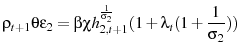
and
Combining the first order equations for the governments problem with respect to capital and consumption yields
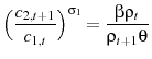
where
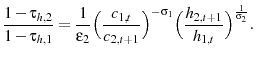
Combining equation 63 and 64 yields
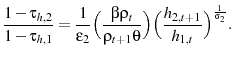
The ratio of first order equations for the government with respect to young and old hours is
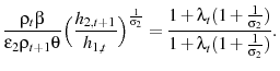
Combining equation 66 and 65 generates the following expression for labor taxes
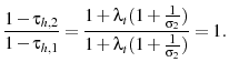 |
(67) |
8.2 LBD
The Lagrangian for this LBD specification is
|
(68) | |
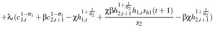 |
where
![\begin{displaymath}\begin{split}\rho_{t}(1+h_{2,t+1}s_{h1}(t+1)) =&\chi h_{1,t}^{\frac{1}{\sigma_{2}}}(1+\lambda_{t}(1+\frac{1}{\sigma_{2}})) -\theta \rho_{t+1} h_{2,t+1} s_{h1}(t+1) \\ &+\lambda_{t} \chi h_{2,t+1}^{1+\frac{1}{\sigma_{2}}}\beta h_{1,t} \Bigg[\frac{s_{h1}(t+1)^{2}}{s_{2}^{2}}-\frac{s_{h2,h2}(t+1)}{s_{2}}\Bigg]\end{split}\end{displaymath}](img276.gif)
![\displaystyle \rho_{t+1}\theta s_{2}=\beta\chi h_{2,t+1}^{\frac{1}{\sigma_{2}}}\Bigg[1+\lambda_{t}(1+\frac{1}{\sigma_{2}})+(1+\frac{1}{\sigma_{2}})\frac{h_{1,t}s_{h1}(t+1)\lambda_{t}}{s_{2}}\Bigg]](img277.gif)
and
The first order conditions with respect to capital and consumption are the same in the exogenous (60, 61, and 62) and LBD models (71, 72, and 73). Therefore equation 14 still holds for this model and therefore the optimal tax on capital is still zero when the government can condition labor income taxes on age.
Combining the first order equations for the governments problem with respect to capital and consumption yields
Taking the ratio of the agent's first order conditions, equations 19 and 20 and combining with equation 74 yields
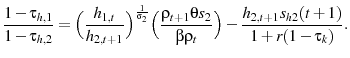
Combining equations 75, 69 and 70 the ratio of the optimal taxes on labor is,
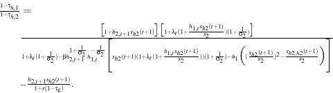 |
(76) |
8.3 LOD
The Lagrangian for the LOD model is
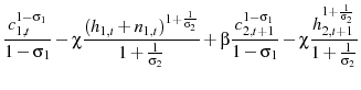 |
(77) | |
|
||
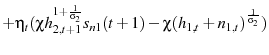 |
where
![\displaystyle \rho_{t}=\chi(h_{1,t}+n_{1,t})^{\frac{1}{\sigma_{2}}}\Bigg[1+\lambda_{t}\Big(1+\frac{h_{1,t}}{\sigma_{2}(h_{1,t}+n_{1,t})}\Big) +\frac{\eta_{t}s_{2}}{\sigma_{2}(h_{1,t}+n_{1,t})}\Bigg]](img282.gif)
![\displaystyle \rho_{t+1}\theta s_{2}=\beta\chi h_{2,t+1}^{\frac{1}{\sigma_{2}}} \Bigg[1+\lambda_{2}\Big(1+\frac{1}{\sigma_{2}}\Big)-\eta_{t}\Big(1+\frac{1}{\sigma_{2}}\Big)s_{n1}(t+1)\Bigg]](img283.gif)
and
| (83) | ||
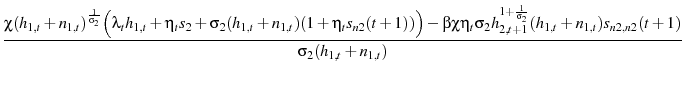 |
(84) |
The first order conditions with respect to capital and consumption are the same in the exogenous (60, 61, and 62) and LOD models (80, 81, and 82). Therefore equation 14 still holds for this model and therefore the optimal tax on capital is still zero when the government can condition labor income taxes on age.
Combining the first order equations for the governments problem with respect to capital and consumption yields
Taking the ratio of the agent's first order conditions, equations 27 and 28 and combining with equation 85 yields
Taking the ratio of equations 78 and 79 yields,
Combining equations 86 and 87 generates the following expression for the ratio of the optimal labor taxes,
 |
(88) |
9.1 LBD Model
Given a social security replacement rate ![]() , a sequence of skill accumulations parameters
, a sequence of skill accumulations parameters
![]() , government expenditures
, government expenditures ![]() , and a sequence of
population shares
, and a sequence of
population shares
![]() , a stationary competitive equilibrium in the LBD model is a sequence of agent allocations,
, a stationary competitive equilibrium in the LBD model is a sequence of agent allocations,
![]() , a production plan for the firm
, a production plan for the firm ![]() , a
government labor tax function
, a
government labor tax function
![]() , a government capital tax function
, a government capital tax function
![]() , a social security tax rate
, a social security tax rate ![]() , a age-specific human capital accumulation function
, a age-specific human capital accumulation function
![]() , a utility function
, a utility function
![]() , social security benefits
, social security benefits ![]() , prices
, prices ![]() , and transfers
, and transfers ![]() such that:
such that:
- Given prices, policies, transfers, and benefits the agent maximizes the following
Max
(89)
subject to![\displaystyle c_{j}+a_{j+1}=ws_{j}h_{j}-\tau_{ss}ws_{j}h_{j},+(1+r)(a_{j}+Tr)-T^{l}[ws_{j}h_{j}(1-.5\tau_{ss})] -T^{k}[r(a_{j}+Tr)],](img290.gif)
(90)
(91)
for, and
(92)
for. Additionally,
(93)
(94) - Prices and satisfy
(95)
(96) - The social security policies satisfy
(97)
(98) - Transfers are given by
(99) - Government budget balance:
![\displaystyle G=\sum_{j=1}^{J}\mu_{j} T^{k}[r(a_{j}+Tr)] + \sum_{j=1}^{j_{r}-1} \mu_{j}T^{l}[ws_{j}h_{j}(1-.5\tau_{ss})]](img296.gif)
(100) - Market clearing:

(101)
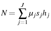
(102)
(103)
9.1.1 LOD Model
Given a social security replacement rate ![]() , a sequence of skill accumulations parameters
, a sequence of skill accumulations parameters
![]() , government expenditures
, government expenditures ![]() , and a sequence of
population shares
, and a sequence of
population shares
![]() , a stationary competitive equilibrium in the LBD model is a sequence of agent allocations,
, a stationary competitive equilibrium in the LBD model is a sequence of agent allocations,
![]() , a production plan for the firm
, a production plan for the firm ![]() , a
government labor tax function
, a
government labor tax function
![]() , a government capital tax function
, a government capital tax function
![]() , a social security tax rate
, a social security tax rate ![]() , a age-specific human capital accumulation function
, a age-specific human capital accumulation function
![]() , a utility function
, a utility function
![]() , social security benefits
, social security benefits ![]() , prices
, prices ![]() , and transfers
, and transfers ![]() such that:
such that:
- Given prices, policies, transfers, and benefits the agent maximizes the following
Max
![\displaystyle _{c_{j},h_{j},n_{j},a_{j+1}}\beta^{j-1}[\prod_{q=0}^{j-1}\Psi_{q}]u(c_{j},h_{j},n_{j})](img300.gif)
(104)
subject to(105)
(106)
for, and
(107)
for. Additionally,
(108)
(109) - Prices and satisfy
(110)
(111) - The social security policies satisfy
(112)
(113) - Transfers are given by
(114) - Government budget balance:
(115) - Market clearing:
(116)
(117)
(118)
Footnotes
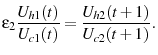 |
(16) |
However, in the analytically tractable model with exogenous human capital accumulation, this constraint is not binding and thus the Lagrange multiplier equals zero. Return to Text
 . Return to Text