
Inflation Risk Premium: Evidence from the TIPS Market*
Keywords: TIPS market, inflation risk premium, expected inflation, term structure of real rates
Abstract:
1 Introduction
Recently there has been a considerable interest in Treasury Inflation-Protected Securities (TIPS) amid concerns about inflation. For instance, according to a recent fund flows update from Morningstar, total net asset values of TIPS funds increased by more than 54% over the one-year period January 2009 - January 2010 and investors added $19.5 billion to TIPS funds during the same period. As we know, both the principal and coupon payments from TIPS are linked to the value of an official price index - the Consumer Price Index (CPI), and as such are denominated in real rather than nominal so TIPS can be considered to be almost free of inflation risk.1 The difference between nominal Treasury and TIPS yields of equivalent maturities is known as a TIPS breakeven inflation rate and represents a compensation to investors for bearing inflation risk.2 This compensation includes both expected inflation and the inflation risk premium due to inflation uncertainty. The focus of this study is to estimate the latter component based on TIPS breakeven rates.
Indeed, as Federal Reserve Board Chairman Bernanke (2004) stressed, estimating the magnitude of the inflation risk premium is important for the purpose of deriving the correct measure of market participants' expected inflation. Furthermore, having a good estimate of the inflation risk premium is important for both the demand and the supply sides of the economy. On the demand side, such a measure would allow investors to hedge effectively against inflation risk. On the supply side, this measure would allow the Treasury to tune the supply of TIPS. The former Federal Reserve Chairman Greenspan (1985) also emphasized the importance of the inflation risk premium: "The real question with respect to whether indexed debt will save taxpayer money really gets down to an evaluation of the size and persistence of the so-called inflation risk premium that is associated with the level of nominal interest rates."
However, the inflation risk premium is not directly observable. The literature on estimating the magnitude and the volatility of the inflation risk premium is also rather limited. Furthermore, there seems no consensus so far on the magnitude of the inflation risk premium and those obtained in the literature have a wide range of values. For instance, some of the estimates, especially those based on a long sample period, are higher than perceived by the Federal Reserve. For instance, Bernanke (2004) comments that "Estimates of the inflation risk premium for bonds maturing during the next five to ten years are surprisingly large, generally in a range between 35 and 100 basis points, depending on the time period studied." On the other hand, estimates based on more recent and shorter sample periods tend to be lower. In addition to the time period studied, the nominal and real term structure models used may be another reason for the wide range of inflation risk premium estimates. Also, there are very few studies of inflation risk premium that are based on TIPS data, which is not surprising to certain extent because the TIPS market is relatively young.
In this paper, we extract the inflation risk premium from TIPS market prices, motivated by the insight of Bernanke (2004) that "the inflation-indexed securities would appear to be the most direct source of information about inflation expectations and real rates." The approach we use to estimate inflation risk premium is a "model free" one in the spirit of Evans (1998), and is arbitrage free. Furthermore, this estimation approach is easy to implement, takes nominal and TIPS yields as given, and does not assume any specifications of the nominal and real term structures. As such, the approach is especially useful for the purpose of obtaining estimates of inflation risk premium.
In our empirical analysis we implement the estimation approach using monthly yields on zero-coupon TIPS and nominal Treasury bonds of 5-, 7-, and 10-year maturities from the Federal Reserve (and also from Barclays Capital) over the period 2000-2008. Depending on the proxy used for expected inflation, we find that in the full sample the average 10-year inflation risk premium ranges from -16 to 10 basis points. Furthermore, the risk premium is found to be negative in the first half of our sample period and this appears to be due to a combination of illiquidity of TIPS and deflation scare in 2002-2003. However, we find that in the second half of the sample period, the inflation risk premium is significantly positive and the 10-year premium varies from 14 to 19 basis points, depending on the proxy used for expected inflation.3 Inflation risk premium is also found to be considerably less volatile during the 2004-2008 period. This indicates that the monetary policy of the Fed has been credible in recent years and inflation expectations are well anchored.
In our analysis we make two adjustments to market prices of TIPS. First, we propose a new liquidity measure based on TIPS prices and provide a liquidity correction for the inflation risk premium. TIPS market is known to contain a sizable liquidity component especially during early years of its
operation (see, e.g., Roll (2004), D'Amico, Kim and Wei (2009), Pflueger and Viceira (2011)). For this reason TIPS yields are biased upward with respect to the true real yields, that are used in deriving
inflation expectations. To measure TIPS liquidity we use an average fitting error of TIPS individual issues' yields with respect to the Svensson (1994) yield curve. Hu, Pan and Wang (2010) provide a rationale for such a measure and apply it to
nominal U.S. Treasury debt market. They argue that in times when capital is abundant the arbitrage forces smooth out the Treasury yield curve so the average fitting errors are low. On the other hand, at the times of scarce capital, investors have harder time to smooth out arbitrage trades and this
results in relatively high fitting errors of the Treasury curve. We apply a similar reasoning to the TIPS market that the divergence of model and market prices represents a shortage of arbitrage capital on the TIPS market, and therefore, proxies for worsening liquidity market conditions.4 Such a measure is attractive because it is based solely on TIPS prices that are also used in the computation of the inflation risk premium. We obtain that our
liquidity measure does not exceed on average 6 basis points in our sample, but exhibits several significant spikes throughout the sample. Such increases (roughly 30![]() 35 b.p.) occur, for
example, between 2002 and 2003 when the number of outstanding TIPS issues was particularly small. Our measure also shows a gradual increase from 2007 to the end of our sample, the end of 2008, when market conditions started to deteriorate significantly.
35 b.p.) occur, for
example, between 2002 and 2003 when the number of outstanding TIPS issues was particularly small. Our measure also shows a gradual increase from 2007 to the end of our sample, the end of 2008, when market conditions started to deteriorate significantly.
Second, we make a distinction between TIPS yields and real yields in order to take into account explicitly the three-month indexation lag of TIPS in the analysis and provide a corresponding estimate. Such a difference between TIPS and real yields is largely ignored in the literature and especially in the financial media. We find that the magnitude of this correction ranges from about 0.03 b.p. for one-year TIPS yields to about 4.2 b.p. for 10-year TIPS. Although the magnitude for the latter looks small, it accounts for a significant portion of the estimated inflation risk premium over long horizons.
To summarize, the main contribution of our study to the literature is to show that we can obtain estimates of inflation risk premium (in the range of 14![]() 19 b.p.) with data on TIPS and
nominal yields, using a simple and easy-to-implement method that is arbitrage free and that otherwise imposes no restrictions on real and nominal term structures.
19 b.p.) with data on TIPS and
nominal yields, using a simple and easy-to-implement method that is arbitrage free and that otherwise imposes no restrictions on real and nominal term structures.
The rest of the paper is organized as follows. Section 2 discusses the studies that form the background for our paper. Section 3 provides an overview of the TIPS market and describes the data used in our empirical analysis. Section 4 describes the methodology. Section 5 presents estimation results for real yields, expected inflation, the inflation risk premium, and compares our results with those in existing studies. Finally, Section 6 concludes.
2 Literature review
Campbell and Shiller (1996) pioneer the approach obtaining estimates of the inflation risk premium using the information from nominal yields (before the arrival of TIPS). Their estimates of the inflation risk premium based on the nominal term premium are between 50 and 100 b.p. Campbell and Viceira (2001) estimate that the inflation risk premium is 35 b.p. in a three-month T-bill and slightly over 1.1% for the 10-year horizon using data on nominal bond prices and inflation over the period 1952-1996. Buraschi and Jiltsov (2005) analyze both nominal and real risk premia of the U.S. term structure of interest rates based on the structural monetary version of a real business cycle model. They find that the 10-year inflation risk premium is on average 0.7% and varies from 0.2% to 1.4% over a 40-year period. Ang et al. (2008) develop a three-factor regime-switching term structure model and estimate the model using nominal rates and inflation data over the period 1952-2004. They document that the unconditional real yield curve is fairly flat around 1.3% but the term structure of inflation risk premium is upward sloping. In addition, they find that the unconditional five-year inflation risk premium is 1.14% on average, but its estimates vary with regimes from 0.42% (in the high real rate regime) to 1.25% (in a regime with higher and more volatile inflation). They also find that the inflation risk premium declined to 0.15% in deflation-scare period after the 2001 recession but started to bounce back to about 1% in December 2004, the end of the sample. Chernov and Mueller (2011) find that inflation risk premia can be positive or negative in their proposed model of the term structure of inflation expectations. Specifically, the premium ranges from 0.2% for one-year to 2% for 10-year maturity when the model is augmented with inflation forecasts from surveys but the range of the estimate becomes -0.07% to -0.3% when no forecast data are used in the model estimation.
Among recent studies using TIPS data, D'Amico, Kim and Wei (2009) consider a three- and four-factor Gaussian term structure model of interest rates and inflation. They estimate the model using realized inflation series, nominal and TIPS yields, as well survey forecasts of short rates. Their estimates of the inflation risk premium are negative and in the range of -1% to -50 b.p. when no liquidity factor is taken into account. However, when the fourth (liquidity) factor is introduced, inflation risk premium estimates become positive and in the range of 0 and 1%, where its magnitude depends on whether liquidity factor is correlated with other factors or not. Adrian and Wu (2010) fit an eight-factor term structure model to both nominal and real yields and also find that the inflation risk premium can be negative. Haubrich, Pennacchi and Ritchken (2011) estimate a term structure model of real and nominal yields using data on nominal Treasury yields, survey forecasts of inflation, and inflation swap rates. Their estimated 10-year inflation risk premium is between 28 and 62 basis points, and on average 48 basis points over the sample period 1982-2009.
Campbell, Shiller and Viceira (2009) argue that TIPS risk premia should be low or even negative. D'Amico et al. (2009) and Wright (2009) reason that the risk premium ought to be positive. Evans (1998) notes that, in general, the inflation risk premium can be positive or negative depending on how the real pricing kernel covaries with inflation. Taking a similar view, Hördahl and Tristani (2007) argue that this correlation translates into a correlation between consumption growth and inflation in some simple models and is negative, implying positive inflation risk premium.5 However, they note that more general models do not necessary result in this simple intuition because in this case the pricing kernel depends on the marginal utility of consumption, not necessarily proportional to consumption growth. In particular, Hördahl, Tristani and Vestin (2007) calibrate a general equilibrium model with habit persistence and nominal rigidities and find that the inflation risk premium is positive and small around one-year maturity and essentially zero for all other maturities.
Campbell et al. (2009) provide a detailed and comprehensive overview of inflation-indexed markets in the U.S. and also in the U.K. In another recent comprehensive survey paper, Bekaert and Wang (2010) note that the estimates of the inflation risk premium in the literature vary depending on the data, models, and methods used. As such, there appears no consensus so far in the literature as to not only the magnitude of the inflation risk premium but also its sign.
Our study complements the aforementioned studies on the inflation risk premium in that we can obtain estimates of the premium using a simple and easy-to-implement method that also takes into account the impact of the indexation lag in TIPS on real yields.6 These estimates are substantially lower than those obtained by Campbell and Shiller (1996), Campbell and Viceira (2001), Buraschi and Jiltsov (2005), Ang et al. (2008), and Haubrich et al. (2011), as well as by D'Amico et al. (2009).
Our inflation risk premium estimates are liquidity corrected ones. The literature on TIPS liquidity is quite scarce as of now, as the market itself is quite recent. D'Amico et al. provide a measure of liquidity premium by introducing a separate (fourth) factor into their term structure model of nominal and real yields. By decomposing liquidity component into deterministic part and stochastic part they find that deterministic trend went down from 120 basis points in 1999 to roughly 10 basis points in 2004 with the stochastic component fluctuating between -50 to 50 basis points. Pflueger and Viceira (2011) use a regression-based approach to estimate liquidity premium. Among their proxies are transaction volume for TIPS, the financing cost for buying TIPS, the 10-year nominal off-the-run spread and the Ginnie Mae (GNMA) spread. Overall, they find that liquidity component varies between 40 and 70 basis points.
However, the results in these studies may not be directly comparable to ours due to differences in sample periods, estimation methods, and data sets used. In particular, our estimates are extracted from TIPS over a more recent and relatively low inflation period. Moreover, we stop our sample in October 2008, the beginning of the financial crisis, to get inflation risk premium estimates during "normal" market functioning period. D'Amico, Kim and Wei (2009) also do not include data beyond March 2007. Gurkaynak and Wright (2010) document that comparable maturity bonds were trading at quite different prices in November and December of 2008 (see Figure 7 in their paper). Fleckenstein, Longstaff and Lustig (2010) also document that TIPS market during that period represented exceptional arbitrage opportunities and that prices were far from being rational ones. These considerations might potentially complicate the inference about inflation risk premium, the focus of our paper.7
3 Data description
In this section we first provide a brief review of the TIPS market and then describe the TIPS and inflation data sets used in our analysis.
Treasury Inflation-Protected Securities (TIPS) were first issued by the U.S. Treasury Department in 1997. Although initially called TIPS, inflation-indexed bonds are now officially referred to as Treasury Inflation Indexed Securities. Nevertheless, market participants keep calling these instruments TIPS, so we retain this abbreviation for our study. The first inflation-indexed debt issue had a maturity of 10 years. Since then the Treasury has been issuing regularly additional 10-year debt, and 5-, 20-, and 30-year debt irregularly. However, the 20-year maturity is replaced by the new 30-year maturity in February 2010. Currently the U.S. Treasury auctions 5-year TIPS in April and October, 10-year TIPS in January, April, July, and October, and 30-year TIPS in February and August.
The TIPS market has been growing significantly since its inception. It is now the world's largest inflation-indexed securities market with over $550 billion of TIPS outstanding and an average daily turnover over $5 billion, and accounts for about 8% of Treasury's marketable debt portfolio (by the Treasury Department's own estimate). To put all this in a perspective, the TIPS market had $450 billion of outstanding, representing roughly 10% of Treasury debt, and an average daily turnover over $8 billion, in September 2007.
Our sample period extends from January 2000 to September 2008. Although data on TIPS before 2000 are also available, we do not include them in the sample due to concerns of the low liquidity in the TIPS market prior to 2000. It is believed that liquidity problems plagued this market in its early period (see, e.g., Roll (2004), Shen (2006), and D'Amico et al. (2009)). In fact, at one time in May 2001 the Treasury Advisory Committee of the Bond Market Association even recommended the TIPS program to be discontinued. We use smoothed data on monthly zero-coupon yields of 5-, 7-, and 10-year maturities for both TIPS and nominal Treasury bonds constructed by Gurkaynak, Sack and Wright (2010) (hence, GSW data) and pulled from the public website of the Federal Reserve Board.8 We have also used TIPS data set from Barclays Capital Bank in some earlier drafts of the paper before the GSW data set became available to general public in 2008. The results are essentially identical so we report only the results based on the GSW data in the analysis that follows. The end point of our sample is motivated by the fact that bond market conditions have deteriorated significantly with in the end of 2008, especially in November and December of 2008, so we have excluded last quarter of 2008 from our sample. Gurkaynak and Wright (2010) discuss bond market functioning around this period.
Panels A and B of Figure 1 plot monthly term structure of nominal Treasury bonds and TIPS, respectively. Observe from the figures that essentially, both nominal and TIPS yields decrease steadily since the beginning of our sample period until 2004. The period of low long-term rates between 2004 and 2006 is often called "conundrum," referring to the fact that the increase in the short-term rates did not lead to a consequent increase in the long-term rates. (The Federal Open Market Committee increased the federal funds rate 17 times from 1% up to 5.25% between June 2004 and June 2006.) The mild increase in nominal and TIPS long-term rates in 2006 and 2007 is associated with the lower volatility of interest rates than in the first half of our sample. Panel C of Figure 1 shows the TIPS breakeven rate defined as the difference between 10-year nominal and TIPS zero-coupon yields. Clearly, the breakeven rate is relatively low and volatile in the first half of the sample and relatively high and less volatile in the second half.
To calculate the inflation risk premium, we need to estimate expected inflation. Our first proxy for expected inflation is the unconditional estimate of inflation forecasts based on two measures of realized inflation. One is the seasonally-unadjusted Consumer Price Index for All Urban Consumers (CPI-U), to which TIPS are linked, and the other is the core CPI (Consumer Price Index Excluding Food and Energy). (We use CPI-U and CPI interchangeably in the paper.)
To construct the second proxy for expected inflation, we entertain a Vector Autoregression (VAR) model to estimate expected inflation, following Ang and Piazzesi (2003) and Chernov and Mueller (2011). We include in the VAR real
activity and inflation variables. Real activity variables include the log growth rates of ![]() - Index of Help Wanted Advertising in the Newspapers,
- Index of Help Wanted Advertising in the Newspapers, ![]() - civil U.S. employment,
- civil U.S. employment, ![]() - industrial production index IP, and, finally,
- industrial production index IP, and, finally, ![]() - the unemployment rate. This represents the standard list of variables used in monthly VARs in macroeconomic literature (see, e.g. Ang and Piazzesi (2003)). Realized inflation variables used in our
VAR include are available on monthly basis. In particular, we include the seasonally-unadjusted consumer price index
- the unemployment rate. This represents the standard list of variables used in monthly VARs in macroeconomic literature (see, e.g. Ang and Piazzesi (2003)). Realized inflation variables used in our
VAR include are available on monthly basis. In particular, we include the seasonally-unadjusted consumer price index ![]() , the Core
, the Core ![]() , and the production price index inflation rate
, and the production price index inflation rate ![]() in our VAR regression.
in our VAR regression.
The third proxy for expected inflation we use is surveys of inflation forecasts. This is motivated by Ang et al. (2007), who find that survey measures forecast inflation the best. One proxy we use is from the Survey of Professional Forecasters (SPF) conducted by the Federal Reserve Bank of Philadelphia every quarter and the other is the Blue Chip Forecasts provided by Aspen Publishers.9SPF forecasts of one- and 10-year ahead inflation are available on a quarterly basis while one-year ahead Blue Chip forecasts are available monthly.
Blue Chip inflation forecasts are not reported in a conventional way. Blue Chip Forecasts of Financial and Economic Indicators represent consensus forecasts of about 50 professional economists in the leading financial and economic advisory firms, and investment banks each month. The survey contains the forecasts of key financial and macroeconomic indicators, including the CPI inflation (inflation hereafter). In particular, Blue Chip Economic Indicators provide monthly estimates of one-year inflation forecast for both the current year and the next year. For instance, in January 1999, Blue Chip provides the expected inflation for both 1999 and 2000. In February 1999, survey participants also provide inflation forecasts for 1999 and 2000, but the forecast horizon is actually 11 months for 1999 and 23 months for 2000. In December 1999, analysts again provide forecasts of the 1999 and 2000 year inflation albeit with a forecast horizon of only one month for 1999 and 13 months for 2000. This feature of the survey results in a time-varying forecast horizon for any variable in question. In our empirical analysis we need monthly forecasts for a fixed horizon. For instance, in February 1999 we need a one-year ahead inflation forecast, but the Blue Chip Survey has only 11-month and 23-month ahead forecasts available. Therefore, we obtain monthly fixed horizon forecast by performing linear interpolations. Similar interpolations are performed in Chun (2011).
We now proceed to the summary statistics of the data used in our empirical analysis, reported in Table 1. The term structure of both nominal and TIPS yields is upward sloping. Average TIPS yields in our sample are between 2.09% and 2.49% for 5- and 10-year index-linked bonds, respectively (Panel A). Average nominal yields are between 4.13% (5-year yields) and 4.82% (10-year yields) in our sample (Panel B). This indicates that the breakeven rate is between 2.04% and 2.33% depending on the maturity. As we mentioned earlier, the breakeven rate is also quite volatile (see Panel C of Figure 1).
Panel C of Table 1 reports statistics of various realized and expected inflation measures. The average realized CPI-based inflation is 2.89% with 0.94% volatility during our sample period, while the average realized core inflation is 2.20% and naturally, has a much lower volatility of only 0.42%, because Core index excludes very volatile energy and food prices. In addition, we report the statistics for Producer Price Index inflation, the variable that we use in the VAR estimation of expected inflation. On average, PPI inflation is 3.24% with 2.57% volatility. Next, we report the descriptive statistics for the Survey of Professional Forecasters (SPF) and Blue Chip Economic Indicators (BCF). SPF includes one- and 10-year forecasts of seasonally-unadjusted CPI and BCF produces one-year ahead CPI forecasts. The SPF forecasts are available quarterly, while BCF forecasts are available monthly. The average forecast of a 10-year CPI inflation rate reported by SPF is 2.49% per year with a standard deviation of only 0.04%. This allows us to proxy the SPF 10-year expected inflation by a single number, 2.5%. The average BCF one-year ahead forecast of the CPI-based inflation is 2.52% with a standard deviation of 0.45%. Note that this one-year forecast is higher than the forecast reported by SPF. Overall, summary statistics reported in Panel C indicates that the measures of realized and expected inflation far exceed the breakeven inflation.
Panel D reports sample summary statistics of the real activity variables that we use in our VAR(1) model for estimating expected inflation. All growth rates in Table 1 are the log differences of the index levels at time ![]() and
and ![]() .
.
4 Methodology
We compute the inflation risk premium as the difference between the nominal-real yield spread and expected inflation. To proceed, we need to estimate both real yields and expected inflation. Notice that TIPS rates are not (true) real rates because TIPS coupon and principal payments are linked to the three-month lagged inflation index, rather than the current inflation index level.10In this section, we first establish a relationship between three term structures: the term structure of nominal rates, the TIPS term structure, and the term structure of real rates, that would allow us to estimate the latter rates. We then present three alternative proxies for expected inflation.
4.1 Notation
Before proceeding with our analysis, we define our notation as follows:
Nominal bonds. Let ![]() denote the time-
denote the time-![]() nominal price of a
zero-coupon bond paying $1 at period
nominal price of a
zero-coupon bond paying $1 at period ![]() . Then the continuously compounded yield on a bond of maturity
. Then the continuously compounded yield on a bond of maturity ![]() is given by
is given by
and the
![\displaystyle F_t(h,k) = \left[ \frac{Q_t(h)}{Q_t(h+k)} \right]^{1/k} - 1.](img20.gif) |
(2) |
Real bonds. Let ![]() denote the nominal price of a zero-coupon bond at period
denote the nominal price of a zero-coupon bond at period ![]() paying
paying
![]() at period
at period ![]() , where
, where ![]() is the (known) price level at
is the (known) price level at ![]() .
. ![]() also defines the real price of one consumption bundle at
also defines the real price of one consumption bundle at ![]() . By definition, such a bond completely indexes against future movements in price levels
. By definition, such a bond completely indexes against future movements in price levels ![]() periods ahead. It then follows that the continuously compounded real yield on a bond of maturity
periods ahead. It then follows that the continuously compounded real yield on a bond of maturity ![]() and the
and the ![]() -period forward rates are respectively given by
-period forward rates are respectively given by
![\displaystyle y^R_t(h) = - \frac{1}{h}\ln Q^R_t(h)\quad \textup{and}\quad F^R_t(h,k) = \left[ \frac{Q^R_t(h)}{Q^R_t(h+k)} \right]^{1/k} - 1.](img24.gif)
Bonds with incomplete indexation. Let
![]() denote the nominal price of an index-linked (IL) zero-coupon bond at period
denote the nominal price of an index-linked (IL) zero-coupon bond at period ![]() paying
paying
![]() at period
at period ![]() , where
, where ![]() is the indexation lag. When
is the indexation lag. When ![]() , then such a bond pays out $1 at maturity. Therefore, we have
, then such a bond pays out $1 at maturity. Therefore, we have
![]() in the absence of arbitrage. The yields and forward rates of IL bonds are as follows:
in the absence of arbitrage. The yields and forward rates of IL bonds are as follows:
![\displaystyle y^{IL}_t(h) = - \frac{1}{h}\ln Q^{IL}_t(h)\quad \textup{and}\quad F^{IL}_t(h,k) = \left[ \frac{Q^{IL}_t(h)}{Q^{IL}_t(h+k)} \right]^{1/k} -1.](img30.gif) |
(4) |
The TIPS indexation lag is three months, so
4.2 Nominal, real, and index-linked term structure
We now proceed to establish the relationship between nominal, IL, and real prices:
![]() and
and ![]() , using the stochastic discount factor approach in the
spirit of Evans (1998). We assume that the price index
, using the stochastic discount factor approach in the
spirit of Evans (1998). We assume that the price index ![]() for the month
for the month ![]() is known at the end of the period
is known at the end of the period ![]() . This seems to be a reasonable approximation of the US data since the index is published with a two-week delay only.
. This seems to be a reasonable approximation of the US data since the index is published with a two-week delay only.
It is known that in the absence of arbitrage opportunities, there exists a stochastic discount factor ![]() such that the one-period nominal returns for all traded assets,
such that the one-period nominal returns for all traded assets,
![]() , are given by
, are given by
where ![]() is the gross return on asset
is the gross return on asset ![]() between
between ![]() and
and ![]() , and
, and
![]() is the expectation conditional on the information set at time
is the expectation conditional on the information set at time ![]() . Namely,
we have for
. Namely,
we have for ![]() :
:
It also follows from (5) that
where
![]() . We can obtain the price of an IL claim in a similar fashion. Given that
. We can obtain the price of an IL claim in a similar fashion. Given that
![]() , we need prices only for IL claims with maturities
, we need prices only for IL claims with maturities ![]() .
It is straightforward to show that
.
It is straightforward to show that
Let lowercase letters stand for the natural logarithms of their uppercase counterparts, e.g.
![]() and
and
![]() . Log-linearizing equations (6), (7), and (8), and applying
. Log-linearizing equations (6), (7), and (8), and applying
![]() , we have:
, we have:
![\displaystyle E_t \left[ \sum^h_{i=1}m_{t+i} \right] + \frac{1}{2}\mathrm{Var}_t\left(\sum_{i=1}^h m_{t+i} \right),](img52.gif)
![\displaystyle E_t \left[\sum^h_{i=1}m^R_{t+i}\right] + \frac{1}{2}\mathrm{Var}_t\left(\sum_{i=1}^h m^R_{t+i} \right),](img54.gif)
![\displaystyle E_t \left[\sum^{\tau}_{i=1}m^R_{t+i} + q_{t+\tau}(l) \right] + \mathrm{Cov}_t\left(\sum^{\tau}_{i=1}m^R_{t+i},q_{t+\tau}(l)\right)](img56.gif)
![\displaystyle + \frac{1}{2}\left[\mathrm{Var}_t\left(\sum_{i=1}^h m^R_{t+i}\right) + \mathrm{Var}_t(q_{t+\tau}(l)) \right],](img57.gif)
where
4.3 Term structure of real interest rates
Now let
![]() , and, in particular,
, and, in particular,
![]() . Using (9), (10), (11), and the definition of
. Using (9), (10), (11), and the definition of
![]() , we can link the log prices of nominal, real, and IL bonds by the following formula:
, we can link the log prices of nominal, real, and IL bonds by the following formula:
where
Eq. (13) shows that the log price of real bonds is not only a function of nominal prices and IL prices, but also depends on
In order to derive the estimates of the real term structure, we rewrite Eq. (12) in terms of yields. Let
![]() and
and
![]() be the continuously compounded yields for nominal, real, and IL bonds, respectively. It follows that:
be the continuously compounded yields for nominal, real, and IL bonds, respectively. It follows that:
As such, in order to estimate real yields
To proceed, we follow the VAR methodology proposed by Evans (1998). We consider the following first-order vector autoregression:
where
where
4.4 Proxies for expected inflation
Recall that in addition to nominal-real yield spreads, we also need expected inflation in order to estimate the inflation risk premium. Below we consider three alternative proxies for expected inflation. We report estimates of expected inflation based on each of the three methods in Section 5.
4.4.1 Expected inflation based on historical average
One straightforward way is to compute expected inflation as the average of historical inflation rates over the past ![]() years. Namely, we estimate a
years. Namely, we estimate a ![]() period expected inflation as follows
period expected inflation as follows

where the
In our empirical analysis, we vary both the estimation horizon
4.4.2 Expected inflation based on the VAR
In the second approach we use a VAR model to estimate expected inflation. Assume that the state vector of the economy is governed by the vector
![]() , where
, where ![]() is the vector of real activity variables, and
is the vector of real activity variables, and
![]() is the vector of inflation variables. We assume further that the state vector
is the vector of inflation variables. We assume further that the state vector ![]() evolves according to the following VAR(1) process:
evolves according to the following VAR(1) process:
where
where
In our empirical implementation, for each date
The use of real activity variables here is motivated by the idea behind Phillips curve that they should be important in predicting inflation. Following Ang and Piazzesi (2003), we form the vector of real activity variables ![]() as follows:
as follows:
![]() , where
, where ![]() is the log growth rate of the
Index of Help Wanted Advertising in the Newspapers,
is the log growth rate of the
Index of Help Wanted Advertising in the Newspapers, ![]() is the log growth rate of civil employment,
is the log growth rate of civil employment, ![]() is the log growth rate of the industrial production index, and
is the log growth rate of the industrial production index, and ![]() is the unemployment rate. Inflation variables used include year-to-year rates based
on
is the unemployment rate. Inflation variables used include year-to-year rates based
on
![]() , and
, and ![]() inflation series, respectively. Namely,
inflation series, respectively. Namely,
![]() .12
.12
4.4.3 Surveys' inflation forecasts
Last, but not least, we use three forecasts of inflation from the Survey of Professional Forecasters and the Blue Chip Economic Indicators. Quarterly Surveys of Professional Forecasters produce one-year ahead and 10-year ahead forecasts. Monthly Blue Chip Economic Indicators data are used to construct one-year ahead forecasts.
As mentioned before, Ang et al. (2007) conclude that surveys outperform other forecasting models and methods. However, Blue Chip Forecasts are not included in their study. In a related study, Chernov and Mueller (2011) include Blue Chip Forecasts among others and conclude that their model, which combines yields and survey data inflation, produces dominating out-of-sample forecasts of both inflation and yields compared with the model where no survey forecasts is included in the model.13
4.5 Inflation risk premium
In order to define the inflation risk premium, consider log-linearized nominal and real yields given by Eqs. (9) and (10), respectively. Using the definition of continuously compounded yields (1) and
(3) and the fact that
![]() , we obtain:
, we obtain:
![\displaystyle -\tau y_t(\tau) = E_t \left[ \sum^{\tau}_{i=1}m_{t+i} \right] + \frac{1}{2}\mathrm{Var}_t\left(\sum_{i=1}^{\tau} m_{t+i} \right)](img112.gif)
and
![\begin{displaymath}\begin{array}{lll} -\tau y^R_t(\tau) & = & E_t \left[ \sum^{\tau}_{i=1}m^R_{t+i} \right] + \frac{1}{2}\mathrm{Var}_t\left(\sum^{\tau}_{i=1} m^R_{t+i} \right) \\ & = & E_t \left[ \sum^{\tau}_{i=1}m_{t+i} + \sum^{\tau}_{i=1}\pi_{t+i} \right] + \frac{1}{2}\mathrm{Var}_t\left(\sum_{i=1}^{\tau} m_{t+i} \right) \\ && \, + \, \frac{1}{2}\mathrm{Var}_t\left(\sum_{i=1}^{\tau} \pi_{t+i} \right) + \mathrm{Cov}_t(\sum^{\tau}_{i=1} m_{t+i},\sum^{\tau}_{i=1} \pi_{t+i}). \end{array}\end{displaymath}](img113.gif)
|
(23) |
Therefore,
![\displaystyle \frac{1}{\tau} E_t \left[ \sum^{\tau}_{i=1}\pi_{t+i} \right] - \frac{1}{\tau} \mathrm{Cov}_t\left(\sum^{\tau}_{i=1}m_{t+i},\sum^{\tau}_{i=1}\pi_{t+i}\right)](img115.gif)
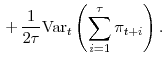
Notice that the first term on the RHS of equation (24) represents the
Using the fact that
![]() we rewrite equation (24) as follows:
we rewrite equation (24) as follows:
where the inflation risk premium (IRP) term is given by
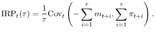
Eq. (25) presents a variation of the Fisher equation and equates the
An alternative approach to estimating the inflation risk premium is to specify the real pricing kernel in a model with a representative agent. Examples of this approach include Fisher (1975), Benninga and Protopapadakis (1983), Evans and Wachtel (1992), Buraschi and Jiltsov (2005), and Hördahl et al. (2007). For the purposes of this paper, we do not specify a stochastic discount factor and instead we use various measures of the expected inflation and the term structure of real and nominal interest rates to infer the inflation risk premium from Eq. (25).
4.6 Liquidity component of the TIPS yield
In this section we propose a measure of illiquidity in TIPS by following Hu, Pan and Wang (2010, HPW), who measure the market illiquidity using the dispersion between observed Treasury nominal yields and the benchmark nominal yields generated from the Nelson and Siegel (1987) and Svensson (1994) model. Specifically, we define the liquidity component of TIPS yields at time ![]() as follows:
as follows:
![\displaystyle y^{L}_t = \sqrt{\frac{1}{N_t}\sum_{i=1}^{N_t}[y^{i,o}_t - y^{i,b}_t]^2},](img121.gif)
where ![]() and
and ![]() represent the observed and benchmark yields,
respectively, of the
represent the observed and benchmark yields,
respectively, of the ![]() -th TIPS at time
-th TIPS at time ![]() , and
, and ![]() is the number of outstanding TIPS date
is the number of outstanding TIPS date ![]() . This measure is not maturity-specific because it is a measure of the
whole TIPS market liquidity. However, it can be maturity dependent if it applies to a particular maturity (or set of maturities) of bonds.14 In our
implementation of this liquidity measure, we calculate the benchmark yields using the Nelson-Siegel-Svensson procedure as well. For brevity, we do not describe this procedure here. See, e.g., Gurkaynak et al. (2010) and HPW for details of the
Nelson-Siegel-Svensson model.
. This measure is not maturity-specific because it is a measure of the
whole TIPS market liquidity. However, it can be maturity dependent if it applies to a particular maturity (or set of maturities) of bonds.14 In our
implementation of this liquidity measure, we calculate the benchmark yields using the Nelson-Siegel-Svensson procedure as well. For brevity, we do not describe this procedure here. See, e.g., Gurkaynak et al. (2010) and HPW for details of the
Nelson-Siegel-Svensson model.
One advantage of the liquidity measure (27) is that it depends only on TIPS prices. Existing liquidity measures for TIPS all depend on the information other than TIPS prices, such as bid-ask spreads and trading volume.
5 Empirical results
In this section we implement the simple estimation approach introduced in Section 4 and present estimates of the real yields, expected inflation, and inflation risk premium. We also correct our estimates of the inflation risk premium for liquidity premium embedded in the real yields and discuss inflation risk premium results when we account for the liquidity premium in the real yields.
5.1 Estimated real yields
In order to compute a real yield, we first estimate first the covariance term
![]() given in Eq. (13), that accounts for the 3-month indexation lag of TIPS. Table 2 reports estimates of
given in Eq. (13), that accounts for the 3-month indexation lag of TIPS. Table 2 reports estimates of
![]() obtained using the VAR(1) model specified in Eq. (15). We provide sample averages of the indexation lag correction in the table. In order to estimate
obtained using the VAR(1) model specified in Eq. (15). We provide sample averages of the indexation lag correction in the table. In order to estimate
![]() for a given
for a given ![]() we use a 10-year sample of
we use a 10-year sample of
![]() and
and ![]() variables prior to date
variables prior to date ![]() in our VAR regression. We repeat the estimation for every
in our VAR regression. We repeat the estimation for every ![]() and then average the obtained
and then average the obtained
![]() estimates. Table 6 reports the averages. Annualized
estimates. Table 6 reports the averages. Annualized
![]() estimates are obtained by multiplying their monthly counterparts by
estimates are obtained by multiplying their monthly counterparts by ![]() . The negative
. The negative
![]() represents the correction to real yields due to the indexation lag. Observe from the table that the estimated negative
represents the correction to real yields due to the indexation lag. Observe from the table that the estimated negative
![]() has a uniformly upward sloping term structure, an indication that the correction is more important for longer maturity TIPS. Intuitively, as
has a uniformly upward sloping term structure, an indication that the correction is more important for longer maturity TIPS. Intuitively, as ![]() increases, uncertainty over the covariance between a longer-term inflation rate
increases, uncertainty over the covariance between a longer-term inflation rate
![]() and a future nominal log price
and a future nominal log price
![]() increases as well. The magnitude of this correction ranges from about 0.03 b.p. for one-year TIPS yields to about 4 b.p. for 10-year TIPS. Although these magnitudes look small,
they account for a significant portion of the estimated inflation risk premium, as can be seen later in Section 5.3.
increases as well. The magnitude of this correction ranges from about 0.03 b.p. for one-year TIPS yields to about 4 b.p. for 10-year TIPS. Although these magnitudes look small,
they account for a significant portion of the estimated inflation risk premium, as can be seen later in Section 5.3.
We then proceed to estimate real yields using Eq. (12). Table 3 reports estimated real yields and also TIPS yields for comparison. Observe first that the former yield is on average indeed lower than the latter yield due to both the forward
rate and indexation lag corrections, and that this difference in yield ranges from around 13 b.p. for the 117-month horizon to about 16 b.p. for the 57-month horizon. Observe also that both real and TIPS yields are significantly higher and also more volatile in the first half of our sample period
January 2000-May 2004 than in the second half from June 2004 until September 2008. For example, in the first half of the sample, real yields on average range from 2.35% to 2.82% depending on the maturity and have an upward-sloping term structure, and the volatility of the real yields on average
ranges from 0.84% to 1.14% per year, and has a downward-sloping term structure. In the second half of the sample, the whole real yield curve shifts downward by around 90 b.p. and is still upward-sloping. The term structure of the real yield volatility on average moves downward by ![]() .
.
The variation over time in real yields shown in Table 3 has implications for both breakeven rates and the estimate of inflation risk premium, the latter the focus of the analysis in Section 5.3. Panel A of Figure 2 plots the 10-year breakeven rate (the nominal-real yield spread) and the SPF 10-year ahead inflation forecast over the entire sample period. Observe that the breakeven rate is relatively low (high) in the first (second) half of the sample period, moving roughly in the opposite direction of the 10-yr real yield. Also, the breakeven rate stays largely below (above) the SPF inflation forecast in the first (second) half of the sample period. This basically implies a negative (positive) inflation risk premium in the first (second) half of the sample period, as the inflation risk premium is typically defined to be the difference between the breakeven inflation rate and expected inflation.
To see if the low breakeven rate in the first subperiod is caused more by low nominal yields or high real yields, we also compute the summary statistics on nominal yields by subperiods. Results (not tabulated) indicate that the nominal yield on average is actually higher in the first subperiod than in the second. The difference in the mean ranges from 9 b.p. for the 117-month horizon to 17 b.p. for the 57-month horizon. This evidence indicates that the low breakeven rate observed in the first subperiod is due to high real yields over the same period.
5.2 Expected inflation estimates
As mentioned before, we consider three alternative proxies for expected inflation: the average of past inflation rates, a VAR based inflation forecast, and the forecast from a professional survey.
Table 4 reports the average of historical inflation rates computed using Eq. (17) over various estimation horizons, based on both seasonally-unadjusted CPI data (Panel A) and Core CPI data (Panel B). Notice that in the table (and also the
subsequent tables), we report the empirical results by bond maturities in months, namely,
![]() , and 117 (month), rather than by years, because corresponding
maturities of TIPS yields and real yields differ by three months (the length of the indexation lag).
, and 117 (month), rather than by years, because corresponding
maturities of TIPS yields and real yields differ by three months (the length of the indexation lag).
We make three observations from Panel A. First, when we use the estimation period of one year (![]() ), the average (proxy for expected inflation here) is mostly flat, around 2.5%,
manifesting the unconditional nature of the estimates. Second, when
), the average (proxy for expected inflation here) is mostly flat, around 2.5%,
manifesting the unconditional nature of the estimates. Second, when ![]() is used in the estimation, the term structure of the expected inflation is upward-sloping. For example, when
is used in the estimation, the term structure of the expected inflation is upward-sloping. For example, when
![]() is used, the expected inflation ranges from 2.47% for the maturity of
is used, the expected inflation ranges from 2.47% for the maturity of ![]() months to 2.72% for the maturity of
months to 2.72% for the maturity of ![]() months. Some other studies obtain similar estimates. In particular, Carlstrom and Fuerst
(2004) find that 10-year ahead expected inflation varies between 2.5% and 2.6%. Finally, when a long estimation horizon,
months. Some other studies obtain similar estimates. In particular, Carlstrom and Fuerst
(2004) find that 10-year ahead expected inflation varies between 2.5% and 2.6%. Finally, when a long estimation horizon, ![]() (that includes periods of high inflation of early and
mid-nineties), is used, the historical average is biased upward and close to 3% per year.
(that includes periods of high inflation of early and
mid-nineties), is used, the historical average is biased upward and close to 3% per year.
Observe from Panel B of Table 4 that the average core inflation rate displays patterns similar to their counterparts shown in Panel A. However, as expected, estimates here are lower than those based on the standard CPI index. On average, 10-year inflation forecasts
based on the estimation period of
![]() and 5 years are around 2.5%.
and 5 years are around 2.5%.
Next, we examine forecasting errors of our three proxies for expected inflation, using seasonally-unadjusted CPI and/or core inflation indices as the benchmark. Table 5 reports the root of the mean squared error (RMSE) calculated for each of the three proxies. Notice
that the RMSE of the survey measure is calculated against only the CPI benchmark as the survey forecasts CPI, but not core CPI. As indicated in the table, the VAR-based forecast has the smallest error, followed by the historical average inflation rate forecast, and then by the survey forecast, at
least in our sample. In particular, the RMSE against CPI ranges from 0.5![]() 0.6 b.p. for VAR-based forecasts, to 10
0.6 b.p. for VAR-based forecasts, to 10![]() 18 b.p. for historical-based forecasts, and as high as 37
18 b.p. for historical-based forecasts, and as high as 37![]() 56 b.p. for surveys' forecasts. Observe also that the RMSE against CPI tends to decrease with the
horizon for the historical mean and surveys' forecasts while VAR-based forecasts lend to almost uniform RMSE across different maturities. However, the opposite pattern is shown for the historical mean and the VAR-based forecast when the core CPI is used as the benchmark. The performance of the
historical mean proxy across the horizon indicates that it can better forecast the more volatile CPI over a longer horizon than a shorter horizon, and can better forecast the less volatile core CPI over a shorter horizon. VAR-based forecast seems to be the most accurate and survey-based forecast -
the least accurate in our sample.
56 b.p. for surveys' forecasts. Observe also that the RMSE against CPI tends to decrease with the
horizon for the historical mean and surveys' forecasts while VAR-based forecasts lend to almost uniform RMSE across different maturities. However, the opposite pattern is shown for the historical mean and the VAR-based forecast when the core CPI is used as the benchmark. The performance of the
historical mean proxy across the horizon indicates that it can better forecast the more volatile CPI over a longer horizon than a shorter horizon, and can better forecast the less volatile core CPI over a shorter horizon. VAR-based forecast seems to be the most accurate and survey-based forecast -
the least accurate in our sample.
There appears no consensus so far in the literature on the best proxy for expected inflation. For instance, Ang, Bekaert and Wei (2007) study several methods for forecasting inflation over the period 1952-2004 and find that surveys outperform other forecasting methods both in-sample and out-of-sample. On the other hand, Chernov and Mueller (2011) find systematic biases in survey forecasts. Nevertheless, they find that surveys along with private sector inflation expectations produce realistic inflation forecasts. However, a comparison of our results with those from these two studies is not straightforward because first, our sample period is different and second, horizons of historical- and VAR-based forecasts are different from those of surveys' forecasts. As such, in the analysis below we consider all of the three proxies examined above for expected inflation.
5.3 Estimation of the inflation risk premium
In this section we present estimates of the inflation risk premium (IRP) obtained using each of three alternative proxies for expected inflation mentioned earlier.15 The first proxy used in our analysis is the average historical inflation rate. The second one is the inflation forecast from the VAR(1) model specified in Eq. (15). Finally, the third proxy is inflation forecasts from the Survey of Professional Forecasters and the Blue Chip Economic Indicators.
Table 6 reports the inflation risk premium estimated over both the full sample and two subsamples, based on each of the three alternative proxies for expected inflation. Observe from the table that the estimates of IRP show several persistent patterns across different inflation forecasts. First, the term structure is upward-sloping regardless of the inflation forecast measure and the sample period used for estimation. Second, both 5- and 7-year CPI-based inflation risk premia are negative over the entire sample as well as over the first half of the sample (Panels A and B). And most of these estimates are statistically significant at the 1% level. The 5- and 7-year core-CPI based inflation risk premia are significantly negative (positive) in the first (second) half of the sample. Third, as can be seen from Panel A, most of the CPI-based 10-year inflation risk premia estimated over the full sample are negative and statistically significant with the exception of the premium based on 1-year CPI forecast reported by the Survey of Professional Forecasters, which is positive and statistically insignificant. The sign and the magnitude of the inflation risk premia based on Core CPI inflation forecast depends on the Core inflation forecast proxy. For instance, the 10-year premium is only -1.4 b.p. (statistically insignificant) in the case of historical-based forecast but is as high as 32 b.p. based on the 1-year VAR Core CPI (at the 1% significance level).
Finally, the 10-year inflation risk premia estimated over the second half of the sample are positive in most cases except when BCF is used as a proxy for expected inflation (Panel C). More specifically, estimates based on CPI inflation forecasts range from 8 b.p. to 13 b.p. And estimates based on core CPI inflation forecasts are much higher, ranging from 38 b.p. to 50 b.p. Both sets of estimates are statistically significant. Obviously, estimates based on core CPI are higher because the core inflation rate on average is lower than the CPI rate. In our sample, the former on average is 2.20% and the latter on average is 2.89% (see Panel C of Table 1).
We also calculate the volatility of the IRP estimates in the two subsamples. Results (not reported) indicate that the estimated IRP is less volatile in the first half of the sample period than in the second.
Figure 3 plots the term structure of the inflation risk premium over time during the entire sample period. The inflation risk premium used in the graph in Panel A (B) is estimated with expected inflation proxied by the average of the historical CPI (core CPI)
rates over the previous five years (![]() ). Both graphs show that the inflation risk premium is visibly negative and relatively more volatile in the first half of the sample but becomes
positive and less volatile in the second half of the sample.
). Both graphs show that the inflation risk premium is visibly negative and relatively more volatile in the first half of the sample but becomes
positive and less volatile in the second half of the sample.
To summarize, we find that the pattern of negative versus positive premia in the two subsamples is robust with respect to the choice of inflation proxy, its horizon, and the estimation period (![]() ) of the historical-based forecasts. This evidence indicates that there seems to be a significant shift in the behavior of the premium around 2003-2004. Also, Adrian and Wu (2010) report a structural break around 2002 (which, they argue, is the turning
point in changing liquidity conditions on the TIPS market). However, what causes such a shift in the level of the inflation risk premium remains an open question. In the next subsection, we consider a few possible explanations.
) of the historical-based forecasts. This evidence indicates that there seems to be a significant shift in the behavior of the premium around 2003-2004. Also, Adrian and Wu (2010) report a structural break around 2002 (which, they argue, is the turning
point in changing liquidity conditions on the TIPS market). However, what causes such a shift in the level of the inflation risk premium remains an open question. In the next subsection, we consider a few possible explanations.
5.4 Liquidity correction
Previous section discusses our estimates of the inflation risk premium without considering a possible bias in the estimates of the inflation risk premium caused by a relative illiquidity of TIPS in the early years of the program. As mentioned before, several studies find that such illiquidity concerns were quite severe. Indeed, D'Amico, Kim and Wei (2009) find that the deterministic trend of the liquidity premium was as high as 120 basis points in 1999 and eventually went down to 10 basis points in 2004. Naturally, illiquidity drives TIPS market prices down and TIPS yields up, and thus, drives a wedge between real yields and TIPS yields. We have corrected TIPS yields for an indexation lag and now correct them for liquidity.
Let
![]() refer to real yield not corrected for liquidity (this one is derived from TIPS yields and adjusted for indexation lag only), and
refer to real yield not corrected for liquidity (this one is derived from TIPS yields and adjusted for indexation lag only), and
![]() refers to real yield, corrected for liquidity. Naturally, the difference between the two is a liquidity correction:
refers to real yield, corrected for liquidity. Naturally, the difference between the two is a liquidity correction:
Therefore, the relationship between nominal, real, expected inflation, and inflation risk premium is given as:
Last equation shows that inflation risk premium estimates might be understated if liquidity adjustment
![]() is ignored. We define the TIPS liquidity adjustment
is ignored. We define the TIPS liquidity adjustment
![]() as the average fitting error (or, noise measure) at each point of time in our sample defined in Eq. (27) in Section 4.6. The notation
as the average fitting error (or, noise measure) at each point of time in our sample defined in Eq. (27) in Section 4.6. The notation ![]() is used here in the loose sense to indicate the bundle of maturities that are used in the construction of this variable.
is used here in the loose sense to indicate the bundle of maturities that are used in the construction of this variable.
We implement empirically this measure using individual observations of TIPS bonds with maturities between 3 and 10 years. As HPW point out, the short end of the curve of the bonds' market is considered to be noisier than other parts of the curve and also unlikely to be an object of arbitrage trades. For this reason, we exclude short maturities observations from the sample to preclude the possibility that our noise measure is driven by the short end effect. HPW use maturities between 1 and 10 years for constructing this measure using nominal Treasuries data. However, short-term TIPS are non-existent, as opposed to nominal Treasuries, and therefore, the fit of the short end of the TIPS curve is highly dependent on the long-term TIPS securities, so we have excluded bonds with maturities less than 3 years.16 When we construct a noise measure, we also exclude outlier observations with yields more than 4 standard deviations away from the sample following HPW. There are less than 2% observations removed from the panel data (456 out of 26,391 bond/day observations). The number of bonds used for construction of noise measure varies from 3 (beginning of our sample) to 16 (end of our sample).
The results of the liquidity adjustment at a monthly and daily frequency are shown on Figure 4, Panels A and B correspondingly. We observe that this measure varies substantially throughout the sample. Panel B shows that there are a few peaks in the daily data in the
sample around 2001 through 2003 (one of the peaks is clearly related to the 9/11 event) with the maximum of roughly 35 basis points in the middle of 2002. We observe that the
![]() is relatively low and stable around 10 basis points between 2005 and 2008. It starts picking up again in 2008 with the development of the financial crisis. While we did not
include the period of the financial crisis in our analysis due to the reasons discussed in Section 3, an extension of our liquidity measure indicates that the noise measure has reached as high as 60 basis points at the pinnacle of the financial crisis.17
is relatively low and stable around 10 basis points between 2005 and 2008. It starts picking up again in 2008 with the development of the financial crisis. While we did not
include the period of the financial crisis in our analysis due to the reasons discussed in Section 3, an extension of our liquidity measure indicates that the noise measure has reached as high as 60 basis points at the pinnacle of the financial crisis.17![]() 18
18
Table 7 presents the results of liquidity estimates. Panel A shows that on average the liquidity measure (27) does not exceed 6 basis points for monthly data and 5 basis points for daily data. The standard deviation of
![]() is around
is around ![]() basis points. The maximum liquidity adjustment
occurs on May 27, 2002 when it reaches 35.12 basis points. Monthly data are extracted from daily data as the last day of each month in the sample. With monthly data, the maximum liquidity adjustment is equal 29.37 basis points. We observe that the average daily
basis points. The maximum liquidity adjustment
occurs on May 27, 2002 when it reaches 35.12 basis points. Monthly data are extracted from daily data as the last day of each month in the sample. With monthly data, the maximum liquidity adjustment is equal 29.37 basis points. We observe that the average daily
![]() is higher in the second half of the sample (Panel C) than in the first half of the sample (Panel B) by about 25 basis points, but the maximum spike occurs still in the first half
of the sample.
is higher in the second half of the sample (Panel C) than in the first half of the sample (Panel B) by about 25 basis points, but the maximum spike occurs still in the first half
of the sample.
The above liquidity correction implies that the estimates of the inflation risk premium in Table 6 have to be adjusted for it. As Eq. (29) shows,
![]() needs to be added to obtain liquidity-adjusted inflation risk premium. Overall, the 10-year liquidity unadjusted inflation risk premium is between -22 to 4 basis points based on
the whole sample (Panel A of Table 6). If we add a monthly average liquidity adjustment to it (5.59 b.p., Panel A of Table 7), we obtain the estimates that vary from -16 to 10 basis points, a finding largely consistent with Adrian and Wu (2010) but obtained using a different and a much simpler method. Similar estimates can be obtained for the first and the second parts of the sample. Panel C of Table 6 reports that the 10-year inflation risk premium varies between 8 and
13 basis points. Adding a monthly average of 5.64 basis points (Panel C of Table 7) we obtain that 10-year inflation risk premium is between 14 and 19 basis points in the second half of our sample 2004:06-2008:09.
needs to be added to obtain liquidity-adjusted inflation risk premium. Overall, the 10-year liquidity unadjusted inflation risk premium is between -22 to 4 basis points based on
the whole sample (Panel A of Table 6). If we add a monthly average liquidity adjustment to it (5.59 b.p., Panel A of Table 7), we obtain the estimates that vary from -16 to 10 basis points, a finding largely consistent with Adrian and Wu (2010) but obtained using a different and a much simpler method. Similar estimates can be obtained for the first and the second parts of the sample. Panel C of Table 6 reports that the 10-year inflation risk premium varies between 8 and
13 basis points. Adding a monthly average of 5.64 basis points (Panel C of Table 7) we obtain that 10-year inflation risk premium is between 14 and 19 basis points in the second half of our sample 2004:06-2008:09.
5.5 Discussion of the results
One main finding of the empirical analysis presented in the previous section is that the inflation risk premium is negative in the period January 2000-May 2004, the first half of our sample period even after we correct for liquidity adjustment. We have two instances when we use survey forecasts to assess inflation expectations and where 10-year inflation risk premium has been positive, but these estimates are not statistically significantly so we still interpret that the first half of our sample results in the negative inflation risk premium.19Although, by definition given in Eq. (26), inflation risk premium can be negative in theory, there might be two reasons for this finding. First reason is that the negative inflation risk premium obtained here still has some liquidity left which is not captured by our TIPS noise measure (28). A higher liquidity premium will result in higher liquidity adjustment and, consequently, bring inflation risk premium to higher levels.
Another possible reason for the negative inflation risk premium in January 2000 - May 2004 is deflation fears during fall 2002 - summer 2003. As chronicled in Bernanke, Reinhart and Sack (2004), the Federal Open Market Committee (FOMC) members began to mention the risks of deflation going forward in the fall of 2002. In response to the concerns about the possibility of deflation in the U.S., the FOMC gradually lowered the federal-funds target rate during this deflation scare until the target was at a 45-year low of 1%. Both nominal and TIPS yields dropped substantially during the same period (see Figure 1). In the mean time, core inflation tumbled from 2% in November 2002 to about 1% one year later. However, as shown in Figure 2, both short- and long-term inflation expectations were still relatively high in that period. As a result, the breakeven inflation rate (namely, the nominal-real yield spread) stayed below the expected inflation during inflation scare, as illustrated in Panel A of Figure 2. This leads to the negative inflation risk premium from the fall of 2002 to the summer of 2003 that we observe in the data.
The estimated inflation risk premium is also negative in the fall of 2008 near the end of our sample period (see Figure 3) although the premium estimated using the entire second half of the sample is positive. (Notice also that both 10-year TIPS breakeven rate and breakeven inflation rate drop substantially at that time, as shown in Panel C of Figure 1 and Panel A of Figure 2, respectively.) As in 2002-2003, deflation scare reportedly occurred in the fall of 2008 after the Lehman default and the onset of the current recession. Several events in connection with the scare are worth mentioning here. First, CPI had a record monthly drop of 1% in October 2008 and the 5-year TIPS breakeven rate became negative for the first time in the same month. Then a November 19 article by Blackstone (2008) posted on the Wall Street Journal's website reported that the Fed Vice Chairman Donald Kohn said on the same day that although still small, the risk of deflation has increased since a few months ago. In addition, the minutes of the FOMC meeting on October 28-29 released also on November 19, 2008 mention that some FOMC members thought an aggressive easing policy should lower the risk of deflation. Yet, another factor that is believed to have influenced the behavior of TIPS during the fall of 2008 is illiquidity or market segmentation between the nominal and TIPS markets. Campbell et al. (2009) and Wright (2009) provide a more detailed discussion of high TIPS yields observed after the Lehman collapse. The latter study, in particular, argues that the inflation risk premium should be positive and that fear of deflation is a potential cause of the negative premium documented empirically. See also Fleckenstein, Longstaff and Lustig (2010) for a description of TIPS market mispricing and potential arbitrage opportunities around that period.
As a result of the above discussion of causes of negative inflation risk premia, we consider the estimates of inflation risk premium obtained over the second half of the sample period to be more reasonable. Furthermore, we focus on estimates relative to CPI but not core CPI as TIPS are indexed to the former. As such, we conclude that the 10-year inflation risk premium ranges between 14 and 19 b.p., depending on the proxy used for expected inflation, based on our empirical analysis and when we correct for liquidity using a liquidity adjustment (28).
These estimates of the inflation risk premium are substantially lower than those obtained by Campbell and Shiller (1996), Campbell and Viceira (2001), Buraschi and Jiltsov (2005), Ang et al. (2008), D'Amico et al. (2009), and Haubrich et al. (2011). On the other hand, our estimates of the 10-year premium are higher than those obtained by some other studies. Ang et al. find that
their estimated inflation risk premium reached a peak of ![]() in the early 1980s, was below 0.5% over 2001-2003, and at one time even declined to 0.15% in 2002-2003 before climbing back to
about 1% in December 2004, the end of their sample (see their Figure 5). Two other studies each obtain different estimates depending on the models and/or data used. Chernov and Mueller (2011) find that inflation risk premia can be positive or negative based on the
model used: their estimates range from 0.2% to 2% when the model is augmented with survey forecasts, while they obtain negative estimates in the range -0.07% to -0.3% when no forecast data is used in the model estimation (see Table 5 in their paper). D'Amico et al. estimate a four-factor Gaussian
term structure model of interest rates and inflation using both nominal and TIPS yields and survey forecasts of short rates. The estimates of the inflation risk premium fluctuate between 0 and 1% in this model.
in the early 1980s, was below 0.5% over 2001-2003, and at one time even declined to 0.15% in 2002-2003 before climbing back to
about 1% in December 2004, the end of their sample (see their Figure 5). Two other studies each obtain different estimates depending on the models and/or data used. Chernov and Mueller (2011) find that inflation risk premia can be positive or negative based on the
model used: their estimates range from 0.2% to 2% when the model is augmented with survey forecasts, while they obtain negative estimates in the range -0.07% to -0.3% when no forecast data is used in the model estimation (see Table 5 in their paper). D'Amico et al. estimate a four-factor Gaussian
term structure model of interest rates and inflation using both nominal and TIPS yields and survey forecasts of short rates. The estimates of the inflation risk premium fluctuate between 0 and 1% in this model.
Our estimates of the inflation risk premium over the full sample period are somewhat consistent with the ones obtained by Hördahl et al. (2007) without using TIPS data, who calibrate a general equilibrium model with habit persistence and nominal rigidities and find that the inflation risk premium is small around 1-year maturity and essentially zero for other maturities. The benefit of our approach is that it is a "model-free" to a large extent and uses information about TIPS yields directly from TIPS market data. Of course, the sign of the inflation risk premium would crucially depend on the model, a measure of inflation expectations and a sample period.
However, we caution against a direct comparison of our results and those obtained in other related studies because different sample periods, estimation methods, and data sets are used in the latter ones. In particular, our estimates are based on TIPS yields over a more recent and relatively low inflation period.
6 Conclusion
This paper represents one of the first attempts to estimate inflation risk premium directly using the prices of Treasury Inflation Protected Securities (TIPS). More importantly, we make distinction between TIPS yields and real yields, taking into account (i) the three-month indexation lag of TIPS, and (ii) liquidity premium embedded in the TIPS yields. We then extract inflation risk premium from the nominal-real yield spread using various measures of inflation expectations.
The estimation approach used in our analysis is arbitrage free, largely model free, and easy to implement. In addition, the implementation of the approach requires only data on historical nominal and TIPS yields, and expected inflation. This approach is especially useful for the purpose of producing market-based estimates of the inflation risk premium. The TIPS liquidity measure proposed here is based on TIPS yields only and very easy to implement.
We find that the 10-year inflation risk premium varies between -16 and 10 basis points over the full sample depending on the proxy used for expected inflation. In addition, the inflation risk premium is found to be time-varying, and more specifically, negative in the first half of our sample period but positive in the second half. Negative inflation risk premium in the first subperiod appears to be due to a combination of illiquidity of TIPS and deflation scare in 2002-2003. In the second half of the sample period, inflation risk premium is significantly positive and the 10-year premium varies from 14 to 19 basis points, depending on the proxy used for expected inflation. The indexation lag correction increases with yield maturity, from 0.03 basis points for one-year TIPS to 4.2 basis points for 10-year TIPS. We also find that the inflation risk premium is considerably less volatile during the 2004-2008 period. This indicates that the monetary policy of the Fed has been credible in recent years and inflation expectations are well-anchored.
We contribute to the literature by obtaining reasonable estimates of inflation risk premium using a very simple method with data on market prices of TIPS and nominal Treasury bonds. Our empirical results should be of value to anyone interested in assessing inflationary expectations and inflation risk premia at a point in time or in tracking changes in those expectations over time.
Bibliography
forthcoming.
forthcoming.
| Central Moment: Mean | Central Moment: Stdev | Central Moment: Skew | Central Moment: Kurt | Autocorrelation: Lag1 | Autocorrelation: Lag2 | Autocorrelation: Lag3 | |
|
|
2.0874 | 0.9927 | 0.4779 | 2.3706 | 0.9737 | 0.9494 | 0.9295 |
|
|
2.3058 | 0.8912 | 0.5769 | 2.3479 | 0.9777 | 0.9574 | 0.9404 |
|
|
2.4930 | 0.7783 | 0.6949 | 2.3478 | 0.9805 | 0.9631 | 0.9482 |
| Central Moment: Mean | Central Moment: Stdev | Central Moment: Skew | Central Moment: Kurt | Autocorrelation: Lag1 | Autocorrelation: Lag2 | Autocorrelation: Lag3 | |
| 4.1299 | 0.9901 | 0.5115 | 2.9097 | 0.9836 | 0.9669 | 0.9516 | |
| 4.4499 | 0.8128 | 0.6931 | 3.1858 | 0.9848 | 0.9698 | 0.9563 | |
| 4.8228 | 0.6511 | 0.8180 | 3.1557 | 0.9860 | 0.9727 | 0.9607 |
| Central Moment: Mean | Central Moment: Stdev | Central Moment: Skew | Central Moment: Kurt | Autocorrelation: Lag1 | Autocorrelation: Lag2 | Autocorrelation: Lag3 | |
| CPI | 2.8864 | 0.9428 | 0.2205 | 2.7029 | 0.9744 | 0.9409 | 0.9113 |
| Core CPI | 2.1984 | 0.4144 | -0.9322 | 3.3338 | 0.9888 | 0.9770 | 0.9639 |
| PPI | 3.2346 | 2.5647 | -0.3752 | 3.4683 | 0.9511 | 0.8930 | 0.8468 |
| SPF, CPI 1yr forecast | 2.3534 | 0.2356 | -0.9290 | 4.2152 | 0.9649 | 0.9289 | 0.8945 |
| SPF, CPI 10yr forecast | 2.4857 | 0.0394 | -2.0119 | 6.5477 | 0.9710 | 0.9421 | 0.9131 |
| Blue Chips, CPI 1yr forecast | 2.5179 | 0.4504 | -0.0791 | 2.4284 | 0.9859 | 0.9694 | 0.9522 |
| Central Moment: Mean | Central Moment: Stdev | Central Moment: Skew | Central Moment: Kurt | Autocorrelation: Lag1 | Autocorrelation: Lag2 | Autocorrelation: Lag3 | |
| EMPLOY | 1.0171 | 1.0126 | -0.2887 | 2.4476 | 0.9529 | 0.9183 | 0.8762 |
| IP | 1.2457 | 2.7200 | -1.1736 | 3.8939 | 0.9121 | 0.8505 | 0.7794 |
| HELP | -17.7050 | 16.0619 | -0.4332 | 2.2716 | 0.9491 | 0.9163 | 0.8854 |
| UE | 5.0743 | 0.6780 | -0.0905 | 1.8605 | 0.9897 | 0.9795 | 0.970 |
This table reports the summary statistics of the data. Panel A reports the statistics on ![]() -month Treasury Inflation Protected Security (TIPS) yields
-month Treasury Inflation Protected Security (TIPS) yields ![]() . Panel B reports statistics on
. Panel B reports statistics on ![]() -month nominal Treasury yields
-month nominal Treasury yields ![]() . Panel C reports the statistics of realized and expected inflation variables. Realized inflation variables are based on the CPI, the seasonally-unadjusted Consumer Price Index for All Urban Consumers (also denoted CPI-U); and
core CPI, the seasonally-adjusted CPI excluding food and energy. We calculate the inflation measure at time
. Panel C reports the statistics of realized and expected inflation variables. Realized inflation variables are based on the CPI, the seasonally-unadjusted Consumer Price Index for All Urban Consumers (also denoted CPI-U); and
core CPI, the seasonally-adjusted CPI excluding food and energy. We calculate the inflation measure at time ![]() using
using
![]() , where
, where ![]() is the inflation index. Expected inflation variables
are: (1) one-year ahead forecast based on CPI price deflator from SPF, (2) 10-year ahead forecast based on CPI price deflator from SPF, and (3) one-year ahead forecast from the Blue Chip Economic Indicators. Panel D reports real activity measures: the growth rates of: (1) the Index of Help Wanted
Advertising in the Newspapers HELP, (2) civil employment level EMPLOY, (3) industrial production index IP, and (4) unemployment rate UE. The growth rate variables are computed as
is the inflation index. Expected inflation variables
are: (1) one-year ahead forecast based on CPI price deflator from SPF, (2) 10-year ahead forecast based on CPI price deflator from SPF, and (3) one-year ahead forecast from the Blue Chip Economic Indicators. Panel D reports real activity measures: the growth rates of: (1) the Index of Help Wanted
Advertising in the Newspapers HELP, (2) civil employment level EMPLOY, (3) industrial production index IP, and (4) unemployment rate UE. The growth rate variables are computed as
![]() , where
, where ![]() is the corresponding level variable. Source: Federal
Reserve Board TIPS and discount bonds data set, Federal Reserve Bank of St. Louis Economic Data Base, Federal Reserve Bank of Philadelphia, Conference Board and Aspen Publishers. The sample period for all variables is 2000:01-2008:09, monthly frequency, except SPF, whose forecasts are
quarterly.
is the corresponding level variable. Source: Federal
Reserve Board TIPS and discount bonds data set, Federal Reserve Bank of St. Louis Economic Data Base, Federal Reserve Bank of Philadelphia, Conference Board and Aspen Publishers. The sample period for all variables is 2000:01-2008:09, monthly frequency, except SPF, whose forecasts are
quarterly.
| Maturity |
Correction to the real yields (in %) due to the 3-month indexation lag of TIPS
|
Correction to the real yields (in %) due to the 3-month indexation lag of TIPS
|
| 12 | -0.0000 | 0.0003 |
| 24 | -0.0000 | 0.0012 |
| 36 | -0.0001 | 0.0027 |
| 57 | -0.0003 | 0.0070 |
| 60 | -0.0004 | 0.0078 |
| 81 | -0.0010 | 0.0154 |
| 84 | -0.0012 | 0.0168 |
| 117 | -0.0038 | 0.0390 |
| 120 | -0.0042 | 0.0418 |
This table reports estimates of
![]() computed as
computed as
![\displaystyle \gamma_t(\tau) = i'_1\left[\sum_{i=1}^{\tau}A^{\tau-i}\left(\sum_{j=1}^i A^{i-j}V(e_{t+j}\vert z_t)A^{i-j'}\right) \right]i_2,](img80.gif)
| Sample period | Horizon |
TIPS yields (%) Mean | TIPS yields (%) Stdev | TIPS yields (%) Skew | TIPS yields (%) Kurt | Estimated real yields (%) Mean | Estimated real yields (%) Stdev | Estimated real yields (%) Skew | Estimated real yields (%) Kurt |
| 2000:01-2008:09 | 57 | 2.087 | 0.993 | 0.478 | 2.371 | 1.928 | 1.018 | 0.460 | 2.363 |
| 2000:01-2008:09 | 81 | 2.306 | 0.891 | 0.577 | 2.348 | 2.173 | 0.910 | 0.572 | 2.371 |
| 2000:01-2008:09 | 117 | 2.493 | 0.778 | 0.695 | 2.348 | 2.367 | 0.790 | 0.740 | 2.465 |
| 2000:01-2004:05 | 57 | 2.518 | 1.105 | -0.070 | 1.693 | 2.352 | 1.141 | -0.064 | 1.691 |
| 2000:01-2004:05 | 81 | 2.783 | 0.946 | -0.127 | 1.680 | 2.639 | 0.983 | -0.112 | 1.676 |
| 2000:01-2004:05 | 117 | 2.973 | 0.787 | -0.112 | 1.681 | 2.817 | 0.840 | -0.064 | 1.680 |
| 2004:06-2008:09 | 57 | 1.648 | 0.613 | -0.295 | 2.004 | 1.495 | 0.639 | -0.302 | 1.986 |
| 2004:06-2008:09 | 81 | 1.819 | 0.478 | -0.286 | 2.107 | 1.698 | 0.498 | -0.308 | 2.119 |
| 2004:06-2008:09 | 117 | 2.004 | 0.348 | -0.151 | 2.104 | 1.908 | 0.360 | -0.181 | 2.122 |
This table reports summary statistics for estimated real yields and also for TIPS yields for comparison. Statistics is reported for both the whole sample and two subsamples. The real yield on a ![]() -month zero-coupon bond,
-month zero-coupon bond, ![]() , is estimated using the following formula:
, is estimated using the following formula:
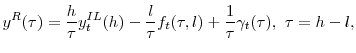
| Estimation period |
Estimation period |
Estimation period |
Estimation period |
Estimation period |
|
| Horizon |
2.514 | 2.463 | 2.469 | 2.528 | 2.722 |
| Horizon |
(0.196) | (0.112) | (0.083) | (0.140) | (0.284) |
| Horizon |
2.498 | 2.484 | 2.526 | 2.635 | 2.839 |
| Horizon |
(0.153) | (0.104) | (0.139) | (0.237) | (0.306) |
| Horizon |
2.551 | 2.612 | 2.718 | 2.837 | 3.028 |
| Horizon |
(0.133) | (0.207) | (0.283) | (0.305) | (0.299) |
| Estimation period |
Estimation period |
Estimation period |
Estimation period |
Estimation period |
|
| Horizon |
2.181 | 2.241 | 2.335 | 2.470 | 2.741 |
| Horizon |
(0.144) | (0.168) | (0.212) | (0.298) | (0.420) |
| Horizon |
2.268 | 2.343 | 2.469 | 2.634 | 2.913 |
| Horizon |
(0.163) | (0.211) | (0.297) | (0.378) | (0.439) |
| Horizon |
2.443 | 2.576 | 2.738 | 2.911 | 3.181 |
| Horizon |
(0.288) | (0.366) | (0.418) | (0.439) | (0.439) |
This table reports the estimates of the expected inflation based on historical average.
![]() is the expected rate of inflation computed as
is the expected rate of inflation computed as ![]() year
historical average of
year
historical average of
![]() ,
, ![]() period realized inflation, computed as
period realized inflation, computed as
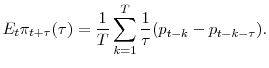
| Proxy for Expected Inflation | Horizon |
RMSE (%) against CPI | RMSE (%) against Core CPI |
| Expected Inflation | (month) | CPI | Core CPI |
| Historical mean: | 57 | 0.1779 | 0.0657 |
| Historical mean: | 81 | 0.1401 | 0.0508 |
| Historical mean: | 117 | 0.0991 | 0.0760 |
| VAR-based forecast: | 57 | 0.0047 | 0.0036 |
| VAR-based forecast: | 81 | 0.0064 | 0.0041 |
| VAR-based forecast: | 117 | 0.0062 | 0.0059 |
| Forecast from surveys: |
12 | 0.5583 | |
| Forecast from surveys: |
120 | 0.4260 | |
| Forecast from surveys: |
12 | 0.3685 |
This table reports the forecasting errors in percentages for the following forecasts of inflation: (1) one-year historical-based forecasts of CPI and core inflation, (2) VAR-based forecasts of CPI and core inflation, and (3) forecasts by the Survey of Professional Forecasters (SPF) and Blue Chip
Economic Indicators of seasonally-unadjusted CPI. One-year historical-based forecasts are computed using the formula (17) and VAR-based forecasts are computed using the formula (20). Seasonally-unadjusted CPI and core inflation are used as the
benchmark. If ![]() is the benchmark inflation and
is the benchmark inflation and ![]() is the forecast series
in question, then the root of the mean squared error (RMSE) is given by:
is the forecast series
in question, then the root of the mean squared error (RMSE) is given by:
| Horizon |
Historical-based CPI 1yr | Historical-based Core 1yr | VAR-based CPI 1yr | VAR-based Core 1yr | Survey-based (CPI only) SPF 1yr | Survey-based (CPI only) SPF 10yr | Survey-based (CPI only) BCF 1yr |
| 57 | -0.357 | -0.024 | -0.514 | 0.015 | -0.238** | -0.370 | -0.361 |
| 81 | -0.259 | -0.029 | -0.313 | 0.107 | -0.153* | -0.285 | -0.279 |
| 117 | -0.123 | -0.014 | -0.218 | 0.325 | 0.042 | -0.090* | -0.089* |
| Horizon |
Historical-based CPI 1yr | Historical-based Core 1yr | VAR-based CPI 1yr | VAR-based Core 1yr | Survey-based (CPI only) SPF 1yr | Survey-based (CPI only) SPF 10yr | Survey-based (CPI only) BCF 1yr |
| 57 | -0.543 | -0.463 | -0.850 | -0.357 | -0.465 | -0.678 | -0.464 |
| 81 | -0.432 | -0.417 | -0.563 | -0.172 | -0.327 | -0.541 | -0.322 |
| 117 | -0.323 | -0.406 | -0.462 | 0.155 | -0.041 | -0.254 | -0.038 |
| Horizon |
Historical-based CPI 1yr | Historical-based Core 1yr | VAR-based CPI 1yr | VAR-based Core 1yr | Survey-based (CPI only) SPF 1yr | Survey-based (CPI only) SPF 10yr | Survey-based (CPI only) BCF 1yr |
| 57 | -0.168 | 0.423 | -0.171** | 0.396 | 0.002 | -0.044 | -0.256 |
| 81 | -0.082* | 0.366 | -0.059 | 0.392 | 0.031 | -0.015 | -0.235 |
| 117 | 0.082 | 0.385 | 0.031 | 0.499 | 0.129* | 0.083 | -0.141 |
This table reports average estimates for the inflation risk premium in percentages based on the following forecasts of inflation: (1) one-year historical-based forecasts of CPI and core inflation, (2) VAR-based forecasts of CPI and core inflation, and (3) forecasts by the Survey of Professional
Forecasters (SPF) and Blue Chip Economic Indicators (BCF) of seasonally-unadjusted CPI. Sample period is January 2000-September 2008. We report quarterly estimates in the case of SPF and monthly estimates in all other cases. Statistics is reported for various subsamples. Estimates at the 1% level
of statistical significance are reported in bold, while estimates at the 5% (10%) level of statistical significance are marked with
![]() .
.
| mean | 4.5933 | 5.5104 |
| st. dev. | 3.4894 | 4.6716 |
| maximum | 35.1184 | 29.3706 |
| mean | 4.8448 | 5.6486 |
| st. dev. | 3.1510 | 4.0546 |
| maximum | 24.3400 | 24.3400 |
This table reports descriptive statistics for the liquidity premium correction defined as a root mean squared error between the market yields ![]() and model-implied yields
and model-implied yields ![]() :
:
![\displaystyle y^L_t(\tau) = \sqrt{\frac{1}{N_t}\sum_{i=1}^{N_t}[y^i_t(\tau) - y^{i,m}_t(\tau)]^2},](img180.gif)
where ![]() is the number of existing TIPS or nominal bonds on date
is the number of existing TIPS or nominal bonds on date ![]() .
.
![]() refers to maturities of the individual bonds, 3 to 10 years, used to compute the liquidity adjustment. Model-implied yields are based on Nelson-Siegel-Svensson functional form. Source:
Federal Reserve Board TIPS data set. Individual bond prices are from Advance Datastream 4.0. Sample period is January 2000-September 2008. The results are reported in basis points for daily and monthly frequency.
refers to maturities of the individual bonds, 3 to 10 years, used to compute the liquidity adjustment. Model-implied yields are based on Nelson-Siegel-Svensson functional form. Source:
Federal Reserve Board TIPS data set. Individual bond prices are from Advance Datastream 4.0. Sample period is January 2000-September 2008. The results are reported in basis points for daily and monthly frequency.
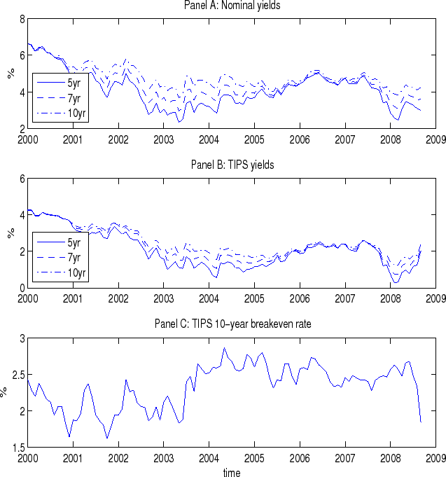 This figure plots zero-coupon nominal (Panel A) and TIPS yields (Panel B) of 5-, 7-, and 10-year maturities, and the 10-year (zero-coupon) TIPS breakeven rate (the zero-coupon nominal-TIPS yield spread) over the period January 2000 - September 2008. |
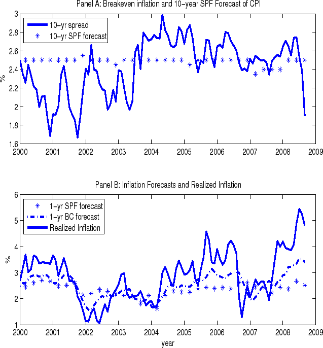 Panel A shows the 10-year breakeven inflation rate (the 10-year nominal-real yield spread) and the Survey of Professional Forecasters 10-year ahead (CPI) inflation forecast. Panel B plots one-year ahead CPI forecasts by the Survey of Professional Forecasters and Blue Chip Forecasters, and realized one-year CPI inflation. The sample period is January 2000 - September 2008. |
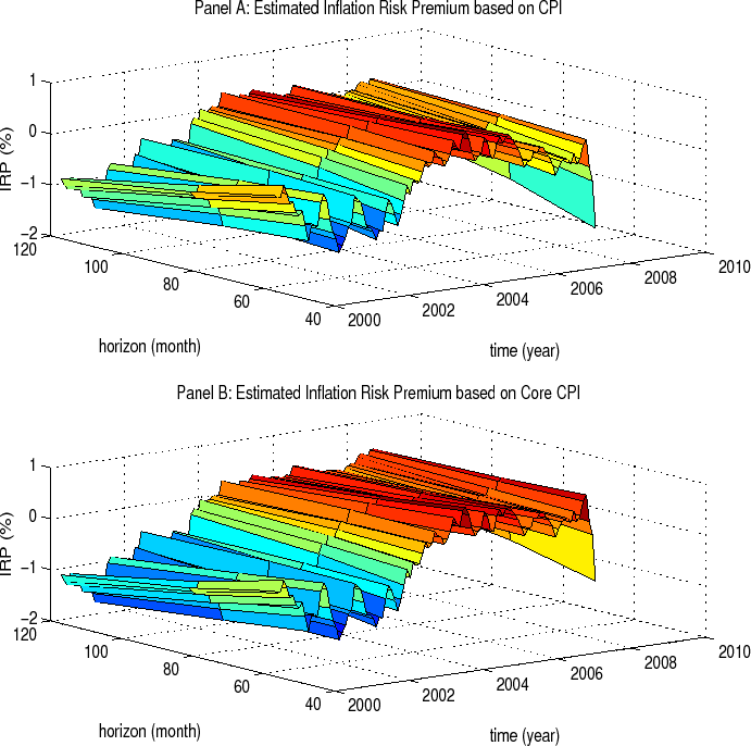 This figure displays the term structure of the inflation risk premium estimated using the historical-based inflation forecast reported in Table 4. Estimation period of inflation forecast used is five years. Panel A shows the inflation risk premium based on the CPI (more precisely, CPI-U). Panel B plots the inflation risk premium based on the seasonally adjusted core CPI (that excludes food and energy prices). Sample period is January 2000 - September 2008, monthly frequency. |
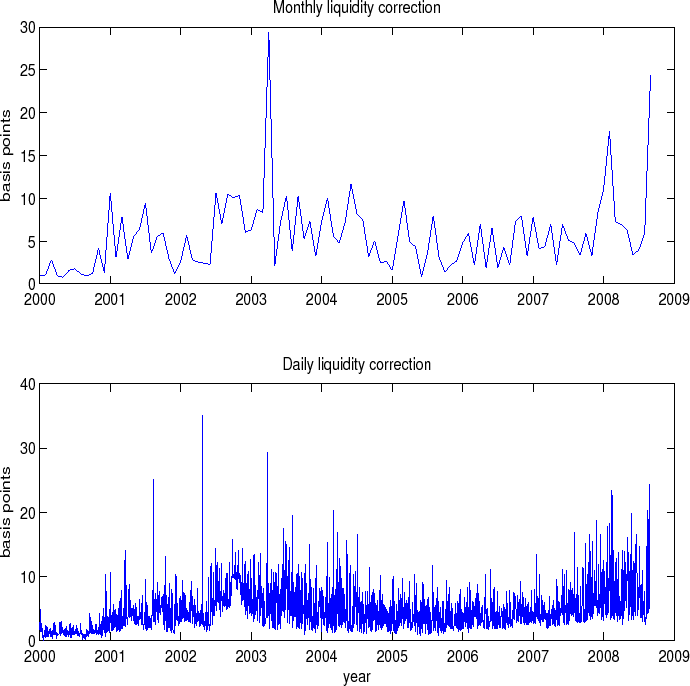 This figure plots liquidity correction embedded in the TIPS yields. Panels A and B display this correction at monthly and daily frequency in basis points, respectively. Liquidity correction is the root mean square error between observed TIPS yields of individual securities and Svensson (1994) model implied TIPS yields of maturities 3 to 10 years. Sample period is January 2000 - September 2008. |