
Misallocation and Financial Market Frictions:
Some Direct Evidence from the Dispersion in Borrowing Costs 1
September 23, 2011
Keywords: Total factor productivity, financial distortions, firms-specific borrowing costs
Abstract:
JEL Classification: D92, O16, O40
1 Introduction
Economists have long emphasized that micro-level distortions can have large adverse effects on aggregate productivity (cf. Hopenhayn and Rogerson [1993] and Guner et al. [2008]). Relatedly, Restuccia and Rogerson [2008] have argued that systematic and persistent differences in the allocation of resources across production units of varying productivity may be an important determinant of differences in income per capita across countries, a hypothesis that seems to be borne out by the data. For example, using detailed microdata on manufacturing establishments in China and India, Hsieh and Klenow [2009] estimate that resource misallocation accounts for 30 to 60 percent of the difference between the total factor productivity (TFP) in U.S. manufacturing and the corresponding sectoral TFP in China and India.5
In light of the enormous differences in the depth and sophistication of financial markets across developed and developing countries, a large literature has long stressed the role of finance in economic development; see Matsuyama [2007] for a comprehensive review. More recently, Amaral and Quintin [2010], Greenwood et al. [2010], and Buera et al. [2011] have developed theoretical models, which show--in a quantitative sense--that a large portion of cross-country differences in TFP may attributable to resource misallocation arising from imperfect financial markets. Although the nature of financial market imperfections differs across their theoretical frameworks, their quantitative analysis shares a common thread, in the sense that the results are obtained by choosing the model parameters to match the size distribution of firms in an environment where financial distortions determine firm size.6
In a recent paper, Midrigan and Xu [2010] challenge these findings. Like Buera et al. [2011], Midrigan and Xu [2010] consider a model in which firms facing financing constraints have a strong incentive to self-finance through forward-looking savings behavior. However, when they calibrate the model to match both the size distribution of firms and the volatility of sales growth, there is simply too little variability in the observed growth of sales to generate quantitatively important differences in the cost of capital across firms. The implication of this result is that financial distortions account for at most 5 percent of the difference in manufacturing TFP between Columbia and South Korea, the latter being a benchmark country with highly developed capital markets.
Although obtaining very different conclusions, the aforementioned studies share a common analytical approach--that is, they identify the size of TFP losses due to resource misallocation using information on the distribution of sales across establishments and over time. In this paper, we provide a direct measure of financial distortions based on the observed differences in borrowing costs across firms. Specifically, we develop an accounting framework in which observed differences in borrowing costs across firms can be mapped into measures of aggregate resource misallocation that may plausibly be attributed to financial market frictions. Using a log-normal approximation, we show that the extent of resource misallocation can be inferred from cross-industry or cross-country information on the dispersion in borrowing costs.
We apply our accounting framework to a panel of U.S. manufacturing firms drawn from the Compustat database. Despite fairly large and persistent differences in borrowing costs across firms, our estimates imply relatively modest losses in TFP owing to resource misallocation--roughly on the order of 3.5 percent of TFP in the U.S. manufacturing sector. Our results can be obtained directly from the log-normal approximation and information on the dispersion of interest rates across firms. Nonetheless, our methodology also allows us to relax the log-normal approximation and infer TFP losses using the joint distribution of sales and borrowing costs. We find that the estimated losses under this approach closely match those obtained under the assumption of log-normality. This finding demonstrates both the robustness of our results, and its applicability to a broader environment where firm-level data on the joint distribution of sales and borrowing costs may not be readily available.
2 Borrowing Costs and Firm Size: Some Some Stylized Facts
In this section, we briefly describe our unique data set on firm-level borrowing costs and present some stylized facts about the relationship between the cross-sectional dispersion in borrowing costs and firm size.
2.1 Data Description
Our main analysis focuses on a subset of U.S. manufacturing firms, whose distinguishing characteristic is that they have access to the corporate bond market. For a panel of such firms covered by the S&P's Compustat and the Center for Research in Security Prices (CRSP), we obtained month-end secondary market prices of their outstanding securities from the Lehman/Warga and Merrill Lynch databases.7 To ensure that we are measuring borrowing costs of different firms at the same point in their capital structure, we limited our sample to senior unsecured issues with a fixed coupon schedule only.
Using the secondary market prices of individual securities, we construct the corresponding credit spreads--measured relative to risk-free Treasury rates--based on the methodology described in Gilchrist and Zakrajšek [2011]. To ensure that our results are not driven by a small number of extreme observations, we eliminated all observations with credit spreads below 5 basis points and greater than 1,000 basis points, cutoffs corresponding roughly to the 2.5th and 97.5th percentiles of the credit spread distribution, respectively. In addition, we eliminated from our sample very small corporate issues (par value of less than $1 million) and all observations with a remaining term-to-maturity of less than one year or more than 30 years. These selection criteria yielded a sample of 2,623 individual securities over the 1985:M1-2010:M12 period. We matched these corporate securities with their issuer's quarterly income and balance sheet data from Compustat and daily data on equity valuations from CRSP, a procedure that yielded a matched sample of 497 firms, split about equally between durable and nondurable goods manufacturing industries.
| Variable | Mean | SD | Min | P50 | Max |
| No. of bonds per firm/month | 2.86 | 3.04 | 1.00 | 2.00 | 52.0 |
| Mkt. value of issue ($mil.)a | 358.9 | 360.1 | 1.22 | 260.4 | 5,628 |
| Maturity at issue (yrs.) | 12.8 | 9.2 | 1.0 | 10.0 | 40.0 |
| Term to maturity (yrs.) | 10.8 | 8.5 | 1.0 | 7.7 | 30.0 |
| Duration (years) | 6.42 | 3.36 | 0.92 | 5.92 | 15.8 |
| Credit rating (S&P) | - | - | D | A3 | AAA |
| Coupon rate (pct.) | 7.06 | 1.97 | 1.70 | 6.85 | 15.25 |
| Nominal effective yield (pct.) | 6.80 | 2.20 | 0.46 | 6.71 | 19.89 |
| Credit spread (bps.) | 170 | 157 | 5 | 116 | 1,000 |
- NOTE: Sample period: 1985:M1-2010:M12; Obs. = 141,770; No. of bonds = 2,623; No. of firms = 497. Sample statistics are based on trimmed data (see text for details).
- aMarket value of the outstanding issue deflated by the CPI (2005 = 100).
Table 1 contains summary statistics for the key characteristics of bonds in our sample. Note that a typical firm in our sample has only a few senior unsecured issues outstanding at any point in time--the median firm, for example, has two such issues trading in any given month. This distribution, however, exhibits a significant positive skew, as some firms can have many more issues trading in the secondary market at a point in time. To calculate a firm-specific credit spread in any given month, we simply average the spreads on the firm's outstanding bonds in that month.8
The distribution of the market values of these issues is similarly skewed, with the range running from $1.2 million to more than $5.6 billion. The maturity of these debt instruments is fairly long, with the average maturity at issue of almost 13 years; the average remaining term-to-maturity in our sample is 10.84 years. In terms of default risk--at least as measured by the S&P credit ratings--our sample spans the entire spectrum of credit quality, from "single D" to "triple A." At "A3," however, the median observation is still solidly in the investment-grade category. An average bond has an expected return of 170 basis points above the comparable risk-free rate, while the standard deviation of 157 basis points reflects the wide range of credit quality in our sample.
We focus on the 1985-2010 period because it is characterized by a growing tendency for U.S. corporate borrowing to take the form of negotiable securities issued directly in capital markets. The resulting deepening of the corporate bond market has led to a substantial degree of disintermediation, as well as to the development of well-functioning markets in derivatives, in which credit, interest rate, and currency risks, for example, can be readily hedged. Importantly, a full-fledged corporate bond market tends to be associated with sound financial reporting systems, a thriving community of professional financial analysts, multiple credit rating agencies, a wide range of corporate debt instruments demanding sophisticated credit analysis, and efficient procedures for corporate reorganization and liquidation, factors that greatly facilitate the process of price discovery for corporate debt claims.9 Indeed, a well-developed corporate bond market is in a much better position than the banking system--which is heavily leveraged and subject to regulatory imperfections--to exert a crucial disciplinary role exercised by market forces.10 As a result, the variation in our firm-specific interest rates likely reflects the dispersion in "true" borrowing costs both across firms and over time.
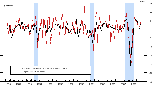
Although our sample is restricted to manufacturing firms with the access to the corporate bond market, these 497 firms account, on average, for about 50 percent of total sales in U.S. manufacturing over the 1985-2010 period. Moreover, as shown in Figure 1, the cyclical fluctuations in their sales closely match the growth of sales of all publicly-traded manufacturing firms in the Compustat database. In combination with the fact that our sample of firms spans a wide range of credit quality (see Table 1), these features of the data suggest that the dispersion if borrowing costs for this subset of firms is likely representative of the manufacturing sector as a whole.
2.2 Firm-Level Borrowing Costs and Firm Size
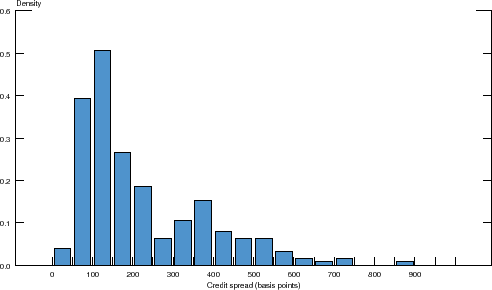
To get a sense of the cross-sectional dispersion in firm-level borrowing costs, we calculate the average credit spread for each firm over time, a measure of debt financing costs that abstracts from the substantial cyclical variation that characterizes credit spreads at business cycle frequencies. The resulting distribution is shown in Figure 2. The central tendency of the distribution--as measured by its mean--is 240 basis points, while its standard deviation is about 160 basis points. Recall that this specific sample trims the upper tail of the distribution of credit spreads at 1,000 basis points, so the standard deviation of 160 basis points likely underestimates the true dispersion of credit spreads across firms to a certain extent.
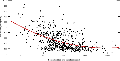
We now turn to the relationship between firm size and credit spreads. In Figure 3, we plot the average credit spread for each firm over time against the average firm size as measured by real sales. The fact that we are averaging over time implies that this relationship is capturing the long-term relationship between firm size and borrowing costs in the U.S. manufacturing sector. The solid line shows the fitted values from regressing the firm-specific average credit spread on a second-order polynomial function of the logarithm of real sales, which highlights the strong negative relationship between firm size and borrowing costs observable in the data.
Credit spreads capture both the likelihood of default and a residual component that relates to firm-specific factors such as loss given default and pricing terms reflecting individual firm characteristics.11 The likelihood of default is intimately related to leverage of the firm. Thus, to the extent that smaller firms are more leveraged, they will be considered by investors as being of lower credit quality and thus face higher spreads in the debt markets.
To control for differences in default risk across firms, we estimate the following regression:
where
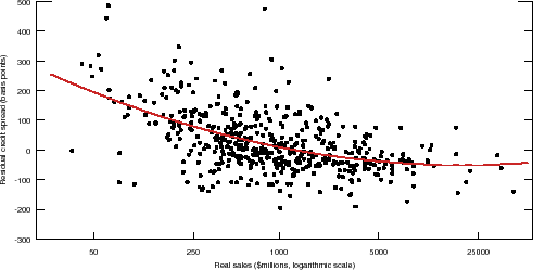
The regression fits the data quite well, explaining 55 percent of the variation in firm-specific credit spreads. In Figure 4, we plot the firm-specific average residual credit spread (i.e.,
![]() ) against the average firm size. Although the dispersion in credit spreads is reduced noticeably once default risk is taken into account, we nevertheless
still find a strong negative relationship between the non-default component of credit spreads and firm size. Such permanent differences in borrowing costs across firms imply that financial distortions play a potentially important role in the misallocation of resources across firms.
) against the average firm size. Although the dispersion in credit spreads is reduced noticeably once default risk is taken into account, we nevertheless
still find a strong negative relationship between the non-default component of credit spreads and firm size. Such permanent differences in borrowing costs across firms imply that financial distortions play a potentially important role in the misallocation of resources across firms.
3 The TFP Accounting Framework
In this section, we present the accounting framework that relates losses in TFP due to resource misallocation to dispersion in firm-specific borrowing costs. Our procedure is derived from the decreasing returns to scale production framework outlined in Midrigan and Xu [2010]; it is also directly related to the TFP accounting procedure emphasized by Hsieh and Klenow [2009].
3.1 The Production Environment
We assume that firms (indexed by ![]() ) employing capital (
) employing capital (![]() ) and labor (
) and labor (![]() ) have access to a decreasing returns to scale production function of the form:
) have access to a decreasing returns to scale production function of the form:
where
We further assume that firms must borrow at a firm-specific interest rate ![]() in order to obtain both capital and labor inputs. Letting
in order to obtain both capital and labor inputs. Letting
![]() denote the rate of capital depreciation and
denote the rate of capital depreciation and ![]() the aggregate
wage, the optimal choice of inputs implies that firms equate the marginal revenue products of capital and labor to their respective costs:
the aggregate
wage, the optimal choice of inputs implies that firms equate the marginal revenue products of capital and labor to their respective costs:
 |
||
where the second equation captures the fact that we assume that labor costs reflect borrowing costs as well as the aggregate wage.
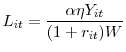
In this framework, the optimal capital-labor ratio is given by
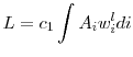
![\displaystyle \frac{K_{i}}{L_{i}} = \frac{1 - \alpha}{\alpha} \left[ \frac{(1+r_{i}) W}{r_{i} + \delta} \right].](img30.gif) |
Solving for the labor input yields
![\displaystyle \frac{\left[(1+r_{i})W \right]}{\alpha \eta} L_{i} = A_{i}^{1 - \eta} \left[ \frac{1 - \alpha}{\alpha} \left(\frac{(1 + r_{i}) W}{r_{i} + \delta} \right) L_{i} \right]^{(1 - \alpha) \eta} L_{i}^{\alpha \eta},](img31.gif) |
which implies the optimal input choices:
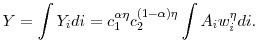
![\displaystyle = c_{1} A_{i} \left[ (1 + r_{i})^{- \frac{1-(1-\alpha) \eta}{1-\eta}} (r_{i} + \delta)^{-\frac{(1-\alpha )\eta }{1-\eta }} \right];](img33.gif) |
||
for some positive constants
Letting
![\displaystyle \equiv \left[ \left(1+r_{i} \right)^{-\frac{1-(1-\alpha) \eta}{1-\eta}} \left( r_{i} + \delta \right)^{-\frac{(1-\alpha )\eta }{1-\eta }} \right];](img39.gif)
![\displaystyle \equiv \left[ \left( 1+r_{i} \right)^{\frac{-\alpha \eta}{1-\eta}} \left( r_{i} + \delta \right)^{-\left( \frac{1-\alpha \eta}{1-\eta} \right)} \right],](img41.gif)
then optimal input choices are proportional to firm-level productivity adjusted for firm-specific differences in factor input costs:
In this context,
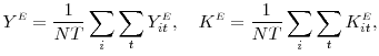
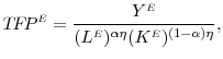
3.2 Aggregation and TFP
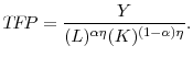
Define aggregate labor and capital inputs according to
 and and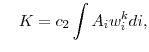 |
and define the wedge in the cost index as
The aggregate output may then be expressed as
 |
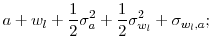
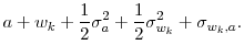
Total factor productivity is measured as aggregate output relative to a geometrically-weighted average of aggregate labor and capital inputs:
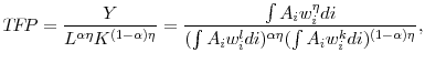 |
or in logs,
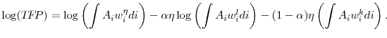
Assuming that ![]() ,
, ![]() , and
, and ![]() are jointly distributed according to a log-normal distribution,
are jointly distributed according to a log-normal distribution,
 MVN MVN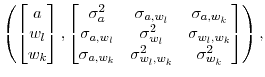
|
then the second-order approximations of the three terms in equation (3) are given by
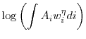 |
![\displaystyle a + \eta \left[ \alpha w_{l} + (1-\alpha) w_{k} \right] + \frac{1}{2} \sigma_{a}^{2} +\frac{\eta^{2} \alpha^{2}}{2} \sigma_{w_{l}}^{2} + \frac{\eta^{2} (1-\alpha)^{2}}{2} \sigma_{w_{k}}^{2}](img58.gif) |
||
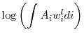 |
 |
||
 |
 |
Combining the above expressions and rearranging yields the second-order approximation of equation (3)
![\begin{displaymath}\begin{split}\log (T\!F\!P) & = (1 - \eta) \left[ a + \frac{1}{2} \sigma_{a}^{2} \right] + \frac{\eta \alpha (1 - \eta \alpha)}{2} \sigma_{w_{l}}^{2} + \frac{\eta (1 - \alpha) (1 - \eta (1- \alpha))}{2} \sigma_{w_{k}}^{2} \\ & \quad - \eta^{2} \alpha (1-\alpha) C\!orr(w_{l},w_{k}) \sigma_{w_{l}} \sigma_{w_{k}}. \end{split}\end{displaymath}](img64.gif)
In an economy with an efficient allocation of resources, ![]() and
and ![]() are constant (i.e.,
are constant (i.e.,
![]() and
and
![]() for all
for all ![]() ). In those circumstances, equation (4) reduces to
). In those circumstances, equation (4) reduces to
![\displaystyle \log (T\!F\!P_{\scriptscriptstyle E}) = (1 - \eta) \left[ a + \frac{1}{2} \sigma_{a}^{2} \right].](img65.gif) |
Hence, the relative TFP loss due to resource misallocation is given by
Several comments about equation (5) are in order. First, the TFP loss due to resource misallocation is an increasing function of the dispersion in the labor and capital wedges
3.3 Resource Misallocation and Dispersion in Interest Rates
To derive an approximate relationship between the dispersion in interest rates and TFP losses due to the misallocation of resources, we first consider a case in which both the labor and capital input choices are fully distorted by financial market frictions (i.e., capital input costs are
![]() and labor input costs are given by
and labor input costs are given by
![]() ). In that case,
). In that case,
![]() , and the log-labor and log-capital wedges are given by
, and the log-labor and log-capital wedges are given by
 |
|||
 |
The first-order approximations of the log wedges around
![\displaystyle - \frac{1}{1-\eta} \left[ (1-(1-\alpha) \eta) \frac{r}{1+r} + \alpha \eta \frac{r}{r+\delta} \right] \log (r_{i});](img78.gif) |
|||
![\displaystyle - \frac{1}{1-\eta} \left[ \alpha \eta \frac{r}{1+r} + \left( 1-\alpha \eta \right) \frac{r}{r+\delta} \right] \log (r_{i}).](img79.gif) |
Thus, the ratio of the standard deviation of the labor wedge relative to the capita wedge can be approximated as
![\displaystyle \frac{\sigma_{w_{l}}}{\sigma_{w_{k}}} \approx \frac{\left[ (1-(1-\alpha) \eta)(r^{2} + r \delta) + (1-\alpha) \eta (r + r^{2}) \right]} {\left[ \alpha \eta (r^{2} + r \delta) + \left( 1 - \alpha \eta \right) (r + r^{2}) \right]}.](img80.gif) |
Because the terms involving
 |
Using this result, we can approximate the expression for the relative TFP loss as a function of
![]() as
as
![\begin{displaymath}\begin{split}\log \left( \frac{T\!F\!P}{T\!F\!P_{\scriptscriptstyle E}} \right) & = \left[ \frac{\eta (1-\alpha) \left[ 1-\eta (1-\alpha) \right]}{2} + \frac{\eta \alpha (1-\alpha \eta)}{2} \left( \frac{(1-\alpha) \eta}{1-\alpha \eta} \right)^{2} \right. \\ & \quad \left. - \; \eta^{2} \alpha (1-\alpha) \frac{(1-\alpha) \eta}{1-\alpha \eta} \right] \sigma_{w_{k}}^{2}, \end{split}\end{displaymath}](img86.gif)
where
![\displaystyle \sigma_{w_{k}} = \frac{1}{1-\eta} \left[ \alpha \eta \frac{r}{1+r} + \left( 1 - \alpha \eta \right) \frac{r}{r+\delta} \right] \sigma_{\log (r)}.](img87.gif) |
The first term in equation (7) reflects the direct effect of variation in
![\displaystyle \log \left( \frac{T\!F\!P}{T\!F\!P_{\scriptscriptstyle E}} \right) = \left[ \frac{\eta (1-\alpha) \left[ 1 - \eta (1-\alpha) \right]}{2} - \frac{\eta \alpha (1-\alpha \eta)}{2} \frac{\sigma_{w_{l}}^{2}}{\sigma_{w_{k}}^{2}} \right] \sigma_{w_{k}}^{2}.](img90.gif)
It is useful to contrast the result in equation (7) with the case where financial market frictions distort only the choice of the capital input, rather than both the capital and labor inputs. In this case,
![]() , and the TFP loss due to resource misallocation is given by
, and the TFP loss due to resource misallocation is given by
![\displaystyle \log \left( \frac{T\!F\!P}{T\!F\!P_{\scriptscriptstyle E}} \right) = \frac{\eta (1-\alpha) \left[ 1 - \eta (1-\alpha) \right]}{2} \sigma_{w_{k}}^{2},](img92.gif)
where
![\displaystyle \sigma_{w_{k}} = \left[ \frac{\left( 1 - \alpha \eta \right)}{1-\eta} \right] \left[ \frac{r}{r + \delta} \right] \sigma_{\log (r)}.](img93.gif) |
Note that for a given
4 Results
In this section, we use our framework to provide some estimates of TFP losses for the U.S. manufacturing sector implied by resource misallocation arising from financial market frictions. Specifically, we use the information on the dispersion of firm-specific borrowing costs to calculate the implied TFP loss, an approach that relies on the assumption of log-normality when computing the second-order approximation of the relative TFP loss. By utilizing the corresponding information on firm-level sales, we show that this approximation provides a reasonable estimate of TFP losses due to resource misallocation.
In our analysis, we assume that the firm-specific borrowing costs in quarter ![]() --denoted by
--denoted by ![]() --are equal to the real risk-free long-term interest rate
--are equal to the real risk-free long-term interest rate ![]() plus the firm-specific premium given by the credit spread
plus the firm-specific premium given by the credit spread ![]() :13
:13
For the real risk-free rate
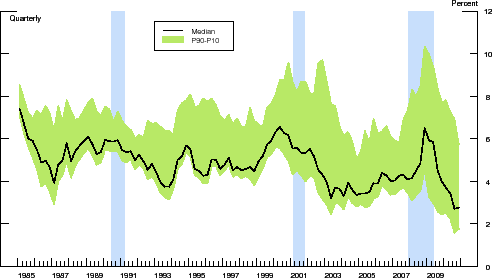
Figure 5 depicts the time-series evolution of the cross-sectional distribution of real interest rates for our sample of manufacturing firms with access to the corporate bond market. The shaded band around the median real interest rate (the solid line) depicts the 90th and 10th percentiles of the distribution of borrowing costs at each point in time. Over the 1985-2010 period, the P90-P10 range has fluctuated in the range between 140 basis and 670 basis points, an indication of a significant dispersion in firm-level borrowing costs.
According to our accounting framework, we can infer
![]() and
and
![]() for each firm in our sample using equations (1) and (2) and the average firm-specific real interest rate
for each firm in our sample using equations (1) and (2) and the average firm-specific real interest rate ![]() . Given these wedges, we can compute their respective standard deviations
. Given these wedges, we can compute their respective standard deviations
![]() and
and
![]() . Using equation (5), we can then calculate the implied TFP loss due to resource misallocation arising from financial market frictions.
. Using equation (5), we can then calculate the implied TFP loss due to resource misallocation arising from financial market frictions.
The above procedure relies only on the cross-sectional dispersion in real interest rates to compute TFP losses due resource misallocation. Given data on firm-level (real) sales--denoted by ![]() --and firm-specific interest rates, it is possible to infer directly the implied capital and labor inputs, according to
--and firm-specific interest rates, it is possible to infer directly the implied capital and labor inputs, according to
 and and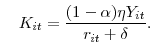 |
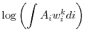
Summing over sales and the implied inputs yields
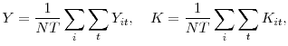 and and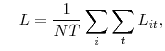 |
which allows us to calculate the implied aggregate TFP:
 |
To infer the level of aggregate TFP that would prevail in the case of the efficient allocation of resources, we first need to compute the firm-specific level of TFP using the relationship
 |
where
where
 and and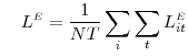 |
denote the aggregate output, capital, and labor that would be obtained under the efficient allocation of resources, the corresponding implied aggregate TFP--the level of TFP that would prevail in the absence of dispersion in borrowing costs--is given by
 |
and the relative TFP loss due to resource misallocation by
 |
Importantly, by using data on firm-specific sales and borrowing costs, we can infer the relative TFP loss due to resource misallocation without relying on the log-normal approximation.
| Sector |
|
|
|
|
Relative TFP Loss Approximate | (Relative TFP Loss Approximate) | Relative TFP Loss Actual | |
| All Manufacturing | 2.43 | 1.16 |
|
0.43 | 0.59 | 1.75 | (3.61) | 3.44 |
| Durable Goods Mfg. | 2.62 | 1.69 |
|
0.43 | 0.60 | 1.77 | (3.65) | 3.23 |
| Nondurable Goods Mfg. | 2.24 | 1.61 |
|
0.42 | 0.58 | 1.69 | (3.48) | 3.63 |
- NOTE: Sample period: 1985:Q1-2010:Q4; No. of firms = 497; Obs. = 16,975. Real interest rates and the implied TFP losses are in percent. The approximate TFP losses use only the information on the dispersion of firm-specific average real interest rates and rely
on the second-order log-normal approximation; the approximate TFP losses reported in parentheses are calculated under the assumption that financial market frictions distort only the choice of the capital input (i.e.,
 ). The actual TFP losses employ information on the firm-specific real interest rates and the corresponding real sales (see text for details).
The results of these two exercises are summarized in Table 2. We calculate the implied TFP losses for all 497 firms in our sample as well as for durable- and nondurable-goods producers separately. The entries under the heading "Approximate" are the
implied TFP losses (in percent) calculated using only the dispersion in the firm-specific borrowing costs and rely on the log-normal approximation; the entries under the heading "Actual" are the implied TFP losses that employ information on both borrowing costs and sales. Columns labeled
![]() ,
,
![]() , and
, and
![]() contain the sample mean, the standard deviation, and the P90-P10 range, respectively, of the average firm-specific borrowing costs,
while
contain the sample mean, the standard deviation, and the P90-P10 range, respectively, of the average firm-specific borrowing costs,
while
![]() and
and
![]() denote the estimates of the cross-sectional standard deviation of the log labor and capital wedges used to compute the approximate TFP losses.
denote the estimates of the cross-sectional standard deviation of the log labor and capital wedges used to compute the approximate TFP losses.
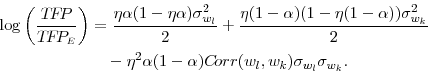
The results in Table 2 indicate that the loss in U.S. manufacturing TFP due to resource misallocation arising from financial market frictions is relatively modest. The losses implied by our approximation method are about 1.75 percent for the manufacturing
sector as a whole and for its two main subsectors. As discussed in Section 3.3, it is possible that in the model where financial frictions distort the choice of both the labor and capital input, the loss in TFP due to resource misallocation is less than the TFP loss in a model where financing
constraints apply only to capital. To evaluate this possibility, we also computed the approximate losses assuming that
![]() , which are reported in parentheses. Note that in all cases, the implied loss in TFP in the absence of financing constraints on labor is about twice as large as the loss
computed under the assumption that financial frictions distort the choice of both inputs. Nevertheless, both sets of estimates imply only a moderate loss in manufacturing TFP due to resource misallocation.
, which are reported in parentheses. Note that in all cases, the implied loss in TFP in the absence of financing constraints on labor is about twice as large as the loss
computed under the assumption that financial frictions distort the choice of both inputs. Nevertheless, both sets of estimates imply only a moderate loss in manufacturing TFP due to resource misallocation.
The actual TFP losses--that is, losses computed using the information on firm-specific borrowing costs and the corresponding sales--are around 3.5 percent for the manufacturing sector as a whole; as before, the estimated losses are highly comparable across the two subsectors. From an economic perspective, however, both methods imply TFP losses that are sufficiently close in magnitude, which suggests that the log-normal approximation, especially under the assumption that financial market frictions do not distort the firm's choice of the labor input, may provide a reasonable estimate of the TFP losses in the case where only information on the dispersion of borrowing costs across firms is available.
With these results in hand, we now consider the implications of two counterfactual scenarios, both of which assume greater dispersion in borrowing costs than actually observed in the U.S. manufacturing data. In the first scenario, we assume that
which roughly doubles the dispersion in firm-level real interest rates; the second scenario counterfactually assumes that
which represents a ten-fold increase in the dispersion of borrowing costs.
| Scenario |
|
|
|
|
Loss | (Loss) | |
| S1:
|
4.84 | 3.30 |
|
0.68 | 0.93 | 4.31 | (8.84) |
| S2:
|
24.2 | 16.5 |
|
1.57 | 1.95 | 19.9 | (39.3) |
- NOTE: Real interest rates and the implied TFP losses are in percent. The approximate TFP losses use only the information on the dispersion of firm-specific average real interest rates and rely on the second-order log-normal approximation; the approximate TFP losses reported in
parentheses are calculated under the assumption that financial market frictions distort only the choice of the capital input (i.e.,
).
As reported in the S1 row of Table 3, doubling the dispersion in firm-specific credit spreads implies an approximate loss in manufacturing TFP of 4.3 percent, assuming that financial market frictions distort the firm's choice of both the capital and labor inputs. Assuming that financing constraints apply only to the capital input, however, implies a TFP loss of almost 9 percent. According to the S2 row, a ten-fold increase in the dispersion of firm-level borrowing costs implies a significant loss in TFP as a result of resource misallocation. Under this counterfactual scenario, the implied loss in TFP, according to our log-normal approximation, is almost 20 percent in the case in which financial frictions distort both the labor market and the market for physical capital. Note, however, that the ten-fold increase in credit spreads that underlies this counterfactual scenario implies an average real interest rate of almost 25 percent, with the P90-P10 range of 8.38 percent to 46.7 percent, extremely high and disperse borrowing costs compared with the actual U.S. data. Indeed, one suspects that they are high even relative to the mean and dispersion in borrowing costs that one is likely to observe in developing economies.
5 Conclusion
This paper developed a simple accounting framework that was used to compute the resource loss due the misallocation of inputs in the presence of financial market frictions. To a second-order approximation, our methodology implies that resource losses may be inferred directly from the dispersion in borrowing costs across firms. Using a direct measure of firm-specific borrowing costs, we show that for a subset of U.S. manufacturing firms, the resource loss due to such misallocation is relatively small--between 1.5 and 3.5 percent of measured TFP. On the whole, our results are consistent with those of Midrigan and Xu [2010], who find that financial market frictions are unlikely to imply large efficiency losses in an economy with relatively efficient capital markets.
Our methodology can easily be used to study the question of what fraction of differences in TFP across countries may be attributable to the misallocation of inputs arising from financial market frictions. Counterfactual experiments indicate that a ten-fold increase in the dispersion in interest rates across firms implies a reduction--through the effect of borrowing costs on resource allocation--in measured TFP of about 20 percent. This finding implies that the dispersion in borrowing costs in developing countries must be an order of magnitude greater than the dispersion of borrowing costs in the United States in order for financial distortions to account for a significant share of the TFP differentials between developed and developing economies.