
A Test for Selection in Matched Administrative Earnings Data*
Keywords: Sample selection, administrative data, survey data
Abstract:
We test whether individuals in the Health and Retirement Study who consented to have administrative earnings data matched to survey responses represent a non-random sample. For both men and women, there is a general pattern of negative selection across three measures of pre-entry labor-market behavior: labor-force participation, self-employment, and earnings. However, for some outcomes the estimates are not precise enough to draw firm conclusions. The strongest results are that men who consented were 4.7 percentage points less likely to be self-employed than those who did not, and women who consented earned 13 percent less than those who did not.
1 Introduction
Administrative records matched to labor-market surveys represent an important innovation in the measurement of earnings. Such data have been compiled for various years of the Current Population Survey, Survey of Income and Program Participation, and the Health and Retirement Study (HRS), and are often gathered for program evaluations. Individuals typically must give informed consent to have their earnings matched. Relatively little is known about whether empirical studies based on the matched earnings of consenters suffer from sample-selection bias, because consenters may display systematically different labor-market behavior than non-consenters. In this paper, we develop a new test for non-random selection in administrative earnings data in the HRS by exploiting the differential timing of the consent process. We apply it to three labor-market outcomes: labor-force participation, self-employment, and log annual earnings.
2 Methods
We illustrate our methods by focusing on earnings. Let true earnings,![]() , be
, be
![]() (1.1)
(1.1)
where ![]() is a vector of explanatory variables, and
is a vector of explanatory variables, and
![]() is the disturbance term. Also, let
is the disturbance term. Also, let ![]() be the net benefit to
individual
be the net benefit to
individual ![]() of consenting,
of consenting,
![]() (1.2)
(1.2)
modeled as a function of observable factors, ![]() , an unobservable monotonic index of the respondent's taste for data privacy,
, an unobservable monotonic index of the respondent's taste for data privacy, ![]() , and a random component,
, and a random component, ![]() . We assume the net benefit is decreasing in privacy,
. We assume the net benefit is decreasing in privacy, ![]() . Define the consent indicator
. Define the consent indicator ![]() as
as
 (1.3)
(1.3)
Then observed earnings (from administrative data),![]() , are
, are
 (1.4)
(1.4)
There will be no sample selection bias to estimates of the determinants of earnings from using the observed sample if
![]() (1.5)
(1.5)
In principle, this could be tested directly by expanding (1.1),
![]() (1.6)
(1.6)
substituting in (1.2) and letting ![]() to yield
to yield
![]() (1.7)
(1.7)
(where
![]() ,
,
![]() , and
, and
![]() ). In this case,
). In this case,
![]() (1.8)
(1.8)
implies no selection bias. Hence, a test of ![]() based on parameter estimates using the sample of observed earnings is a test for sample-selection bias. Unfortunately, in practice this
test typically is not feasible, because
based on parameter estimates using the sample of observed earnings is a test for sample-selection bias. Unfortunately, in practice this
test typically is not feasible, because ![]() is unobserved.
is unobserved.
In our approach, we estimate a variant of (1.7) using a discrete-valued proxy for ![]() that we obtain from the differential timing of the HRS consent process. Specifically, we analyze the
Original Cohort (OC), who entered the HRS in 1992. They are comprised of individuals born 1931-41 and their spouses (regardless of age). At entry, OC individuals were asked consent to link their survey responses to pre-entry administrative data on W-2 earnings and Form 1040 Schedule C
self-employment income through 1991 (Olson, 1999; Bricker and Engelhardt, 2008). This is the initial consent (IC). Three-quarters of respondents consented (tabulated by sex in columns 1 and 2 in Table 1). This group has the lowest index values of
that we obtain from the differential timing of the HRS consent process. Specifically, we analyze the
Original Cohort (OC), who entered the HRS in 1992. They are comprised of individuals born 1931-41 and their spouses (regardless of age). At entry, OC individuals were asked consent to link their survey responses to pre-entry administrative data on W-2 earnings and Form 1040 Schedule C
self-employment income through 1991 (Olson, 1999; Bricker and Engelhardt, 2008). This is the initial consent (IC). Three-quarters of respondents consented (tabulated by sex in columns 1 and 2 in Table 1). This group has the lowest index values of ![]() . Then in 2004-6, individuals were asked consent to match earnings through 2003. This is the subsequent consent (SC). An additional 5.4% of those who did not consent at entry
subsequently did. This group had the next lowest index values of
. Then in 2004-6, individuals were asked consent to match earnings through 2003. This is the subsequent consent (SC). An additional 5.4% of those who did not consent at entry
subsequently did. This group had the next lowest index values of ![]() . The remaining 19.6% of individuals never consented (NC). They had the highest values of
. The remaining 19.6% of individuals never consented (NC). They had the highest values of
![]() . Therefore, the multiple consent process established an ordering:
. Therefore, the multiple consent process established an ordering:
![]() (1.9)
(1.9)
We use this to define an indicator,
 (1.10)
and use it as a proxy for ![]() in (1.7) to yield
in (1.7) to yield
![]() (1.11)
(1.11)
We estimate the parameters in (1.11) using the observed sample. Importantly, differential timing of consent gives variation in ![]() within the observed sample, with which to identify
within the observed sample, with which to identify
![]() . Then we test the null hypothesis that
. Then we test the null hypothesis that ![]() (no difference in
labor-market behavior between initial and subsequent consenters) versus the alternative that
(no difference in
labor-market behavior between initial and subsequent consenters) versus the alternative that
![]() .
.
We test separately for men and women, because of well-established differences by sex in work behavior. The vector ![]() includes standard earnings determinants: a quadratic in age, dummy
variables for race (white and black, respectively), educational attainment (high school degree or GED, some college, college graduate, respectively), whether foreign-born, married, veteran status (for men), and a constant.
includes standard earnings determinants: a quadratic in age, dummy
variables for race (white and black, respectively), educational attainment (high school degree or GED, some college, college graduate, respectively), whether foreign-born, married, veteran status (for men), and a constant.
3 Results and Discussion
Table 2 gives selected descriptive statistics on the three consent groups. Panel A shows means for our three outcome variables from the pre-entry administrative data (1991). The first row of panel B shows the self-reported labor force participation rate from the entry-wave survey (1992). The
second row of that panel shows the percentage of respondents who had item non-response for self-reported earnings via a "don't know" or "refusal." For men and women, this percentage is lowest for initial consenters (IC), higher for subsequent consenters (SC), and highest for never consenters (NC). This is consistent with the assumed ordering in (1.9), and (if the non-response is strategic) would suggest that respondents have similar tastes for earnings privacy in both matched and survey data. The third
row shows that self-reported earnings among the sub-sample with no item non-response generally falls across the consent groups, whereas imputed earnings are more flat (fourth row), not inconsistent with negative selection. Finally, panel C shows means for the demographic characteristics in
![]() and reinforces the findings from Haider and Solon (2000) that there are some, but not particularly large, observable differences in earnings determinants between consenters and
non-consenters.
and reinforces the findings from Haider and Solon (2000) that there are some, but not particularly large, observable differences in earnings determinants between consenters and
non-consenters.
Table 3 presents probit estimates of ![]() in (1.11) for pre-entry (in 1991) labor-force participation, defined as having positive annual earnings or self-employment income. Standard
errors are in parentheses; marginal effects are in square brackets. For brevity, the other parameter estimates are not shown. The estimate of
in (1.11) for pre-entry (in 1991) labor-force participation, defined as having positive annual earnings or self-employment income. Standard
errors are in parentheses; marginal effects are in square brackets. For brevity, the other parameter estimates are not shown. The estimate of ![]() in column 1 for men indicates that,
conditional on standard determinants of labor-market behavior, there is small, negative selection on participation. Men who consented at entry had an estimated 1.7 percentage point lower participation rate than those who subsequently consented. However, this effect is not different than zero at
conventional significance levels. Even if it were, this is an economically small effect relative to the labor-force participation rate of the subsequently matched of 76.7% (panel 3 of Table 1). The results are qualitatively similar for women, shown in column 2.
in column 1 for men indicates that,
conditional on standard determinants of labor-market behavior, there is small, negative selection on participation. Men who consented at entry had an estimated 1.7 percentage point lower participation rate than those who subsequently consented. However, this effect is not different than zero at
conventional significance levels. Even if it were, this is an economically small effect relative to the labor-force participation rate of the subsequently matched of 76.7% (panel 3 of Table 1). The results are qualitatively similar for women, shown in column 2.
In Table 4, we restrict the sample to those in the labor force and present probit estimates of ![]() in (1.11) for pre-entry self-employment, defined as positive Schedule C income. The
marginal effects in column 1 for men indicate selection: entry consenters had an estimated 4.7 percentage point lower self-employment rate than subsequent consenters (p = 0.046), an economically sizable effect relative to the self-employment rate of the subsequent
consenters of 19.5% (panel 3 of Table 1), i.e., almost a 25% increase in the self-employment rate. The estimate for women in column 2 is similar in relative magnitude, but less precise.
in (1.11) for pre-entry self-employment, defined as positive Schedule C income. The
marginal effects in column 1 for men indicate selection: entry consenters had an estimated 4.7 percentage point lower self-employment rate than subsequent consenters (p = 0.046), an economically sizable effect relative to the self-employment rate of the subsequent
consenters of 19.5% (panel 3 of Table 1), i.e., almost a 25% increase in the self-employment rate. The estimate for women in column 2 is similar in relative magnitude, but less precise.
Next, we limit the sample to those in the labor force and not self-employed, then examine the extent of selection in pre-entry log annual earnings. Figures 1 and 2 show unconditional non-parametric kernel density estimates of the distributions of log earnings by consent phase for men and women, respectively, based on an Epanechnikov kernel. Although visually there are some differences between groups, non-parametric tests (Kolmogorov-Smirnov and Wilcoxon Rank-Sum) fail to reject the null hypothesis that entry and subsequent consenters came from the same earnings distribution for each sex.
Table 5 presents OLS estimates of ![]() in (1.11) for log annual earnings as the labor-market outcome. For men, entry consenters had 3.3% lower earnings, than subsequent consenters. These
effects are economically small in magnitude and not statistically different than zero at conventional significance levels.
in (1.11) for log annual earnings as the labor-market outcome. For men, entry consenters had 3.3% lower earnings, than subsequent consenters. These
effects are economically small in magnitude and not statistically different than zero at conventional significance levels.
To explore impacts across the earnings distribution, we estimated the parameters in (1.11) for each quantile of the conditional distribution using the least absolute deviations (LAD) estimator. The solid line in Figure 3 shows the associated estimate of ![]() in (1.11) for each (whole-numbered) quantile. The dashed lines demarcate the boundaries of the 95% confidence interval based on 299 bootstrap replications. For men, there is little evidence of selection across the earnings
distribution.
in (1.11) for each (whole-numbered) quantile. The dashed lines demarcate the boundaries of the 95% confidence interval based on 299 bootstrap replications. For men, there is little evidence of selection across the earnings
distribution.
For women, the OLS estimates of ![]() in (1.11) with log annual earnings as the outcome are shown in column 2 of Table 5. Entry consenters had 13% lower earnings than subsequent
consenters, economically large and statistically different than zero at the 10% significance level. The LAD estimates of
in (1.11) with log annual earnings as the outcome are shown in column 2 of Table 5. Entry consenters had 13% lower earnings than subsequent
consenters, economically large and statistically different than zero at the 10% significance level. The LAD estimates of ![]() in Figure 4 indicate this negative selection effect is spread
evenly across the earnings distribution.
in Figure 4 indicate this negative selection effect is spread
evenly across the earnings distribution.
An issue that arises with our method is that the subsequent consenters are drawn from the pool of respondents still active in the study in 2004-6, many years after entry. This group itself is potentially selected through differential mortality and attrition from the study. As a robustness check, we re-did the empirical analysis limiting the analysis sample to initial and subsequent consenters who were still in the study in 2006, and the results were qualitatively and quantitatively similar.
4 Conclusion
Over the last twenty years, there has been a well-documented decline in household survey response rates and respondent cooperation. This has led to greater efforts to match administrative data to survey responses, in an effort to mitigate measurement error and bolster data quality. We present a method to test for non-random selection in administrative earnings that relies on differential timing of the informed consent process that is typically required for administrative data linkages. The method is applicable for longitudinal surveys that use multiple attempts to obtain consent.
References
Bricker, Jesse and Gary V. Engelhardt, "Measurement Error in Earnings Data in the Health and Retirement Study," Journal of Economic and Social Measurement 33:1 (2008): 39-61.
Haider, Steven J., and Gary Solon, "Nonrandom Selection in the HRS Social Security Earnings Sample," Working Paper No. 00-01, RAND Labor and Population Program, 2000.
Olson, Janice A., "Linkages with Data from Social Security Administrative Records in the Health and Retirement Study." Social Security Bulletin 62 (1999): 73-85.
Table 1. Construction of the Sample by Consent Phase and Sex
| Sample | (1) Men | (2) Women |
| Number in Cohort | 5,812 | 6,730 |
| Without Matched Social Security Records as of 2006 | 1,189 | 1,277 |
| % Unmatched | 20.5% | 19.0% |
|---|---|---|
| With Matched Social Security Records as of 2006 | 4,623 | 5,453 |
| % Matched | 79.5% | 81.0% |
| Number with Matched Social Security Records | 4,295 | 5,109 |
| % Initially Matched | 73.9% | 75.9% |
| Out of the Labor Force in 1991 | 903 | 1,697 |
| In the Labor Force in 1991 | 3,392 | 3,412 |
| With Self-Employment Income | 509 | 281 |
| ii. No Self-Employment Income | 2,883 | 3,131 |
| Number with Matched Social Security Records | 328 | 344 |
| % Subsequently Matched | 5.6% | 5.1% |
| Out of the Labor Force in 1991 | 62 | 116 |
| In the Labor Force in 1991 | 266 | 228 |
| With Self-Employment Income | 52 | 22 |
| No Self-Employment Income | 214 | 206 |
| Variable | (1) Men : Initial Consent | (2) Men : Subsequent Consent | (3) Men : Never Consent | (4) Women: Initial Consent | (5) Women: Subsequent Consent | (6) Women: Never Consent |
| Pre-Entry Labor-Market Activity (1991) from Administrative Data : In the Labor Force (%) | 79.0 | 81.1 | - | 66.8 | 66.3 | - |
|---|---|---|---|---|---|---|
| Pre-Entry Labor-Market Activity (1991) from Administrative Data : Self-Employed (%) | 11.9 | 15.6 | - | 5.5 | 6.4 | - |
| Pre-Entry Labor-Market Activity (1991) from Administrative Data : Earnings ($) | 22,023 | 22,071 | - | 10,840 | 12,414 | - |
| Entry-Wave Labor-Market Activity (1992) from Self-Reported Data: In the Labor Force (%) | 71.6 | 76.8 | 71.4 | 62.3 | 63.1 | 59.5 |
| Entry-Wave Labor-Market Activity (1992) from Self-Reported Data: Earnings Item Non-Response (%) | 7.7 | 19.2 | 23.8 | 7.4 | 14.5 | 17.3 |
| Entry-Wave Labor-Market Activity (1992) from Self-Reported Data: Earnings, Conditional on No Item Non-Response ($) | 27,348 | 24,947 | 23,963 | 12,073 | 12,866 | 10,734 |
| Entry-Wave Labor-Market Activity (1992) from Self-Reported Data: Earnings, Including Imputations for Item Non-Response ($) | 27,645 | 25,652 | 26,534 | 12,728 | 14,231 | 12,617 |
| Demographics: White (%) | 75.8 | 66.2 | 70.1 | 73.0 | 61.6 | 62.5 |
| Demographics: Black (%) | 13.9 | 17.7 | 17.2 | 16.4 | 19.2 | 22.7 |
| Demographics: High School (%) | 35.3 | 32.6 | 31.6 | 41.2 | 33.1 | 37.7 |
| Demographics: Some College (%) | 18.7 | 18.0 | 18.9 | 19.0 | 23.0 | 20.6 |
| Demographics: College Graduate (%) | 19.7 | 18.3 | 20.9 | 13.9 | 17.2 | 13.2 |
| Demographics: Foreign-Born (%) | 9.9 | 12.8 | 10.6 | 10.5 | 15.7 | 13.9 |
| Demographics: Married (%) | 87.6 | 90.2 | 84.9 | 76.1 | 75.9 | 74.5 |
| Demographics: Age (Years) | 55.9 | 55.9 | 55.7 | 52.7 | 52.5 | 52.7 |
| Demographics: Veteran (%) | 56.9 | 50.0 | 55.4 | - | - | - |
Table 3. Probit Estimates of Labor-Force Participation by Sex, Standard Errors in Parentheses, Marginal Effects in Brackets
| Explanatory Variable | (1) Men | (2) Women |
| Initial Consent | -0.067 | 0.024 |
| Initial Consent (standard error) | (0.088) | (0.074) |
| Initial Consent [marginal effects] | [-0.017] | [0.008] |
Note: Standard errors in () and marginal effects in []
Table 4. Probit Estimates of Self-Employment by Sex, Standard Errors in Parentheses, Marginal Effects in Brackets
| Explanatory Variable | (1) Men | (2) Women |
| Initial Consent | -0.187 | -0.106 |
| Initial Consent (standard error) | (0.093) | (0.120) |
| Initial Consent [marginal effects] | [-0.047] | [-0.017] |
Note: Standard errors in () and marginal effects in [].
Table 5. OLS Parameter Estimates for Log Earnings by Sex and HRS, Standard Errors in Parentheses
| Explanatory Variable | (1) Men | (2) Women |
| Initial Consent | -0.033 | -0.130 |
| Initial Consent (standard error) | (0.072) | (0.079) |
Note: Standard errors in ()
Figure 1: Kernel Density Estimates of the 1991 Earnings Distribution for Working Men in the Original Cohort by Match Phase.
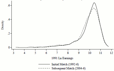
Figure 2: Kernel Density Estimates of the 1991 Earnings Distribution for Working Women in the Original Cohort by Match Phase.
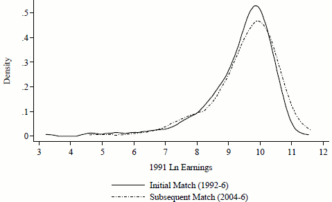
Figure 3: Quantile Regression Estimates and 95% Confidence Interval of Initial Match on 1991 Log Earnings for Men in the Original Cohort.

