Small Price Responses to Large Demand Shocks*
Abstract:
JEL classification: E30, L11.
Keywords: Demand shocks, inflation, sales, labor conflicts, mass population displacement, severe weather events.
1 Introduction
The effect of movements in aggregate demand on prices and quantities remains a lingering question in macroeconomics. A key reason is that prices and quantities are simultaneously determined; analyses based on correlations between these two variables may thus suffer from biases in coefficients and not be used to support causal claims. Ultimately, of course, it is the causal relationship that most interests scholars.1
In this paper, we document a number of instances in which large demand shocks can be identified and show that, in those instances, the level of prices and retailing strategies more broadly react proportionally little. In particular, we study the pricing response of U.S. supermarkets to large demand shocks--that is, shocks that either profoundly reshape the customer base or that alter shoppers' willingness to consume--brought about by labor conflicts, mass population relocation, and shopping sprees caused by severe weather events. As we shall argue, we see the occurrence of our shocks as exogenous to retailers' pricing strategies and supply factors, allowing us to use them as instruments to assess the causal effect of broad-based variation in demand on prices.2
We perform our analysis using a large dataset of weekly scanner data made available to researchers by Information Resources Inc. (IRI). This dataset contains price and quantity information from 2001 through 2011 on 29 personal care, housekeeping, and food products, and is well suited for our endeavor for several reasons. First, it covers 50 U.S. metropolitan markets, making possible the study of shocks that had a large impact on demand at a regional level but a limited influence on national aggregates. Second, its exceptionally large size--about 4 million individual observations per week after our trimming--permits the computation of reasonably accurate statistics at the product category-market level; this feat would not be achievable using the considerably smaller micro datasets collected for the computation of the official CPI and national account statistics. Third, it contains the universe of items sold by stores within each product category, thus allowing us to track the evolution of spending on these categories. In conjunction with the price data, the spending data permit us to derive real (same-store) quantity measures using a methodology similar to that employed for the national accounts. Fourth, the weekly data frequency allows us to zoom in on shocks that have a short life-span. Fifth, the availability of data from multiple retail chains and stores permits us to contrast the pricing behavior of local competitors facing differing shocks to demand.
Our most crucial task is to identify events that can broadly move demand but that are otherwise exogenous to supply factors. We first consider two labor conflicts that both began in October 2003. The conflict in St. Louis, MO, was relatively short (less than a month) while the conflict in Southern California dragged on nearly five months to become the longest supermarket strike and lockout in U.S. history. Affected stores remained open during both conflicts. Because many shoppers would rather take their business elsewhere than cross picket lines, strikes and lockouts can profoundly reshaped store frequentation within a market. Many stores in our sample saw their revenues collapse 50 percent or more for the duration of these conflicts while others experienced correspondingly large increases. Stores whose employees were not on strike or locked-out faced no supply constraints, making the rise in their demand akin to an exogenous demand shock. At the end of the conflicts, staff numbers normalized but store frequentation did not always revert to pre-conflict levels, providing additional opportunities to study the effects of variation in demand.
We next consider the mass population displacement brought about by Hurricane Katrina, the most expensive natural disaster in U.S. history. The hurricane displaced about 1 million persons, many of whom took years to resettle. Most displaced households moved in with relatives or friends, boosting population density and store frequentation in neighborhoods that were less affected by the storm. Stores in our sample from the New Orleans, Louisiana, market and the Mississippi market experienced a persistent rise in sales volumes of about 20 percent, on average, in the wake of the hurricane.
Finally, we consider shopping sprees around major snowstorms and hurricanes not associated with mass population displacement. Like Hurricane Katrina, their occurrence is unquestionably exogenous to retailing activities. But contrary to Hurricane Katrina, the typical effects of these storms on demand are short-lived and operate primarily through a rise in the demand of existing shoppers rather than through a reshuffling of the consumer base. Storms that result in the closing of schools and workplaces force households to consume a larger fraction of their meals at home, thus boosting demand for food items. Similarly, the demand for personal care and housekeeping products may rise as households engage in more home production or take advantage of their trip to the supermarket to purchase items other than food.
Our key finding is that large swings in demand appear to have, at best, a modest effect on the level of prices, consistent with a flat short- to medium-term supply curve in the retail industry. This finding holds even in the case of our most persistent shocks for which stores adjusted the price of most items multiple times (or at least a couple of times in the case of regular prices). Put differently, the lack of a significant price response to large swings in demand seems inconsistent with the marginal cost of retailers being sensitive to the level of demand because of fixed factors of production, or to retailers making large alterations to their markups in response to changes in demand. Our evidence is further consistent with tit-for-tat behavior in which retailers with radically different demand shocks nonetheless seek to match their local competitors' pricing movements and recourse to sales and promotions.
Our two labor conflicts feature the most dramatic shocks to demand in our study. For the Southern California strike and lockout, we split establishments into two broad groups: those that saw a drop in revenues in excess of 10 percent and those that saw an increase in excess of 10 percent (henceforth generically referred to as "on strike" and "not on strike," respectively). The group on strike saw quantities sold drop by half relative to the pre-strike period while the group not on strike saw quantities increase by a third. Despite this remarkable difference, the level of prices was similarly behaved between the two groups throughout the conflict, rising about two percent in the first couple months and erasing half of that increase in the remaining months. These price movements are not especially large relative to the historical volatility of the sample. Importantly, they are modest relative to quantity developments. Perhaps remarkably given limited staffing numbers, stores on strike put almost the same number of items on sale during the conflict, supporting the view that engaging in price discrimination is a central activity of retailers.
At the end of the Southern California conflict, stores that had been on strike recouped only 4 out of every 5 dollars in lost business. To regain market share, these stores increased the number of sales and promotions, a move that was largely mimicked by their local competitors. This strategy gradually brought customers back even though relatively aggressive discounts did not translate into lower transaction prices on average. This finding points to marketing having an influence on sales volumes that goes beyond what can be inferred from movements in price indexes alone.
The shorter St. Louis conflict had similarly large effects on quantities at stores on strike and stores not on strike than the longer Southern California conflict. However, the end of the strike brought an immediate return to pre-conflict activity levels even though the strike had arguably lasted long enough to induce consumers deterred by picket lines to shop at unaffected establishments. Perhaps as a result, stores that had been on strike did not launch a sales and promotion campaign in the wake of the conflict. Overall, these findings suggest that there is some stickiness in consumer preferences for particular points of purchase, that those preferences are not eroded by shopping elsewhere for a few weeks, but that longer displacements such as during the Southern California strike can lead to permanent changes.
We break down the effects of Hurricane Katrina on retail activities in two phases. In the week of the storm, store revenues in our New Orleans sample jumped by nearly a quarter from their average of the previous couple months. The jump was especially sizable for a number of personal care products such as toothbrushes, a sad reminder of the personal tragedies endured by many displaced families. The second phase extends from the weeks after the storm, when store revenues were about 20 percent above average, to well over a year later as displaced households slowly returned home or settled elsewhere. We find little if any evidence that retailers responded to the persistent increase in demand by raising prices. Although food prices rose a little more in New Orleans than the corresponding national average in the months after the disaster, the price of personal care and housekeeping products rose by somewhat less. Moreover, we cannot exclude the possibility that supply disruptions created some upward pressure on food prices in New Orleans, further reducing the contribution of higher demand to the observed food price increase.
Our last set of demand shocks--shopping sprees triggered by major snowstorms and hurricanes--has no apparent effect on prices and other elements of our retailers' pricing strategies. This finding is perhaps unsurprising because weather forecasts suffer from considerable uncertainty even for horizons as short as a few days. Moreover, the effect of these shocks on demand rapidly dissipates. The fleeting character of these shocks may simply leave retailers insufficient time to adjust prices accordingly. Nonetheless, they invite us to qualify earlier findings that retail prices tend to fall around periods of peak demand. Warner and Barsky (1995), MacDonald (2000), Chevalier, Kashyap, and Rossi (2003) report that prices of household appliances and some food items tend to decline around major holidays, which are also short-lived peaks in demand.3 This evidence has been used by a number of authors as suggestive of counter-cyclical markups at the macroeconomic level. Our conjecture is that the high predictability of demand peaks due to holidays or the passing of the seasons allows retailers to adjust their marketing strategies accordingly, making these events somewhat uninformative about how retailers might respond to other high-demand episodes.
To our knowledge, our focus on broad-based demand shocks is novel in the empirical literature that uses large datasets of individual data to bridge micro price behavior and aggregate price dynamics. Perhaps one exception is Coibion, Gorodnichenko, and Hong (2012), who look at the link between local labor market conditions and pricing. Otherwise, previous work has considered a number of supply-related factors such as changes in sales taxes (see, for example, Dhyne et al. (2005) and the references therein, Karadi and Reiff (2012), and Gagnon, López-Salido, and Vincent (2013)), imported good price shocks (for example, Gopinath and Itskhoki (2010)), and commodity price shocks (for example, Nakamura (2008) and Hong and Li (2013)). This literature has typically found moderate pass-through rates that contrast with the muted price responses to our shocks. Our use of natural disasters to identify exogenous changes in demand is also somewhat unusual as the literature has typically been interested in their disruptive effects on supply. In a related paper, Cavallo, Cavallo, and Rigobon (2013) use online price data to show that a 2010 earthquake in Chile and the 2011 Sendai earthquake and tsunami in Japan both led to widespread product unavailability but not to higher prices.
The paper is organized as follows. Section 2 details the construction of our dataset and presents key features of retail activities in normal times, which we will use as a reference to assess the impact of our demand shocks. Section 3 analyzes customer base displacement due to labor conflicts. Section 4 investigates shifts in demand due to major weather events, starting with the year-long population displacement caused by Hurricane Katrina and proceeding with transitory boosts to demand related to major snowstorms and hurricanes. Section 5 concludes.
2 Retail pricing in normal times
Our price and quantity analysis is performed using weekly scanner data made available to researchers for a nominal fee by IRI. The content of the dataset is detailed in Kruger and Pagni (2008) and Bronnenberg, Kruger, and Mela (2008), so we shall give only a brief exposition. The data come from a large sample of over 1,500 U.S. supermarket stores belonging to a variety of retail chains and operating in 50 U.S. markets. An observation corresponds to the information about an item (that is, a barcode sold in a particular store) in a given week. The number of observations is exceptionally large at about 300 million per year. Available item information includes the number of units sold and total revenue during the week. As is customary with scanner data, we derive a unit price by dividing total revenue by the number of units sold. Although the data are limited to 29 food, housekeeping, and personal care products, they have the appealing feature of encompassing all item transactions within those product categories.4
To make the micro data suitable for our purposes, we drop items with suspiciously large price adjustments and apply various filters to extract regular, sales, and reference price series. We then construct price and quantity indexes for each IRI market-product category combination using a methodology that closely matches that employed by the Bureau of Labor Statistics (BLS) and the Bureau of Economic Analysis (BEA) for the U.S. CPI and the U.S. National Income and Product Accounts, respectively. We relegate these technical details to an appendix.
2.1 Central features of retail pricing in normal times
We begin by describing the general behavior of retail prices in the dataset to provide us with a benchmark against which to compare pricing behavior in the presence of large demand shocks. The key message is threefold: retail prices are adjusted frequently, price adjustments are primarily associated with sales and promotions, and the bulk of barcode-level price variation is common across stores belonging to the same retail chain.
Fact #1: Retail prices are adjusted frequently
Table 1 presents some key statistics on posted price adjustments broken down by product category.5
On average, we are able to compute a posted price change for nearly 4 million items each week, which are associated with weekly revenues of about $110 million. Of these items, ![]() percent experience a (nonzero) posted price adjustment.6 The
weekly frequency of price changes is nontrivial for all product categories, ranging from 13.7 percent for sugar substitutes to 43.9 percent for carbonated beverages. When we use only weekly price observations corresponding to the 15th day of each month, we derive a mean monthly frequency of price changes of 42.3 percent. Again, all product categories display frequent price adjustments, with sugar substitutes having the lowest monthly frequency, at 27.5 percent,
and frozen dinner prices having the highest monthly frequency, at 55.2 percent. The mean monthly frequency of price changes in our sample is noticeably higher than corresponding estimates for
the U.S. CPI, which range from about 26 percent in Bils and Klenow (2004) and Nakamura and Steinsson (2008), to about 36 percent in Klenow and Kryvtsov (2008). This difference is not due to the IRI sample being tilted toward product categories that have relatively high frequencies of price changes; if we restrict the CPI sample to personal care and processed food categories, we
find a mean frequency similar to that of the full IRI basket. Instead, the IRI sample's relatively high frequency of price changes likely reflects a selection of stores that are actively changing prices.
percent experience a (nonzero) posted price adjustment.6 The
weekly frequency of price changes is nontrivial for all product categories, ranging from 13.7 percent for sugar substitutes to 43.9 percent for carbonated beverages. When we use only weekly price observations corresponding to the 15th day of each month, we derive a mean monthly frequency of price changes of 42.3 percent. Again, all product categories display frequent price adjustments, with sugar substitutes having the lowest monthly frequency, at 27.5 percent,
and frozen dinner prices having the highest monthly frequency, at 55.2 percent. The mean monthly frequency of price changes in our sample is noticeably higher than corresponding estimates for
the U.S. CPI, which range from about 26 percent in Bils and Klenow (2004) and Nakamura and Steinsson (2008), to about 36 percent in Klenow and Kryvtsov (2008). This difference is not due to the IRI sample being tilted toward product categories that have relatively high frequencies of price changes; if we restrict the CPI sample to personal care and processed food categories, we
find a mean frequency similar to that of the full IRI basket. Instead, the IRI sample's relatively high frequency of price changes likely reflects a selection of stores that are actively changing prices.
Fact #2: Retail price adjustments are primarily driven by sales
A majority of price changes in our sample are associated with sales. To establish this fact, we identify sales using a version of the filter proposed by Nakamura and Steinsson (2008) that eliminates temporary downward price movements. (See the appendix for the details of our implementation.) Table 2 shows that a relatively modest share ( 11.2 percent) of regular prices are adjusted in a typical week, consistent with two out of every three price adjustments in our sample being driven by sales and promotions. The pre-eminence of sales in price adjustments is found in all product categories. On a monthly basis, 23.7 percent of regular prices are adjusted, so that sales account for about half of monthly price adjustments. The fact that sales represent a noticeably smaller fraction of monthly price adjustments than of weekly price adjustments indicates that many sales-related price movements are missed when data are collected monthly.
We also experimented with identifying low-frequency price movements using the concept popularized by Eichenbaum, Jaimovich, and Rebelo (2011) of a "reference price," which we define as an item's modal price over a centered 13-week window. Deviations from reference prices are even more common than deviations from regular prices. At a weekly frequency, references prices are adjusted only 4.5 percent of the time, implying that roughly six out of seven price adjustments in our sample are transitory deviations from the reference prices. At a monthly frequency, reference prices are adjusted 15.6 percent of the time, consistent with over two thirds of monthly price adjustments being transitory deviations from reference prices.
Fact #3: Most prices are set at the retail chain level
Price behavior in the IRI sample is consistent with pricing decisions originating principally at the retail chain level. To establish this fact, we define a weekly "chain price" as the modal price at which a barcode is sold across stores belonging to the same retail chain. Because we cannot link retail chains across IRI markets, our chain price measure is necessarily market-specific even though retail chains may be active in several IRI markets. To ensure that we have a meaningfully large sample of stores to compute a chain price, we require that a barcode's weekly posted price be observed at a minimum of five stores belonging to the same retail chain, in addition to imposing that items are frequently traded (see the appendix for the details of our data cleaning). If there is more than one modal price, then we use the largest one as the chain price. These methodological choices are immaterial for our finding that most pricing decisions do not originate at the store level.
Table 3 presents our key statistics on retail chain pricing. Overall, 71.2 percent of posted prices equal their corresponding chain price, a clear indication that the level of posted price is coordinated to some degree across stores belonging to the same retail chain. This conclusion applies to all product categories in our sample, with the lowest proportion being a still-substantial 65.8 percent in the case of carbonated beverages. It also applies to regular prices, for which we find similar proportions of prices matching the modal regular price of their barcode across stores belonging to the same retail chain. We also find evidence of an appreciable degree of coordination in the timing of price adjustments. As noted earlier, about 30 percent of posted prices are adjusted in a typical week. However, the probability of an item experiencing a price change jumps to over 80 percent when we condition on a change in the item's chain price. (Here we exclude the item's own price from the computation of the chain price to avoid creating a spurious increase in the price change probability.) In sharp contrast, if there is no adjustment in the chain price, then the item has only a 12.3 percent probability of being adjusted. As was the case with the level of prices, the finding of strong coordination in price changes across stores belonging to the same retail chain applies to all product categories and is found for both posted and regular prices.
Summing up, the strong synchronization across stores in the level of prices and the timing of their adjustments indicates that stores play a relatively minor role in the determination of prices in our sample. This finding is consistent with Nakamura (2008), who explores similar issues using a multi-market sample of about 100 barcodes in 2004 from AC Nielsen. She reports that 65 percent of the variation in the level of prices is common across stores belonging to the same retail chain, while only 17 percent is specific to the store and product. Additionally, because the time series variation in item prices is greater than the variation in barcode-level averages, she argues that the large shocks driving retail prices generally do not arise at the manufacturer level.
Other aspects of the data
Tables 1 and 2 show that downward nominal price adjustments are nearly as common as upward price adjustments, a finding that holds true whether one focuses on either posted prices or regular prices. In addition to being frequent, posted price adjustments are also large. On average, the mean weekly posted price increase is 17.6 percent whereas the mean posted price decrease is a little larger at 18.7 percent. Regular price increases and decreases are somewhat smaller, at 12.0 percent and 14.5 percent, respectively.
3 Labor conflicts as exogenous demand shocks
Labor conflicts can have substantial effects on store frequentation because many shoppers would rather take their business elsewhere than cross employee picket lines. Thus, affected stores can lose most of their demand whereas unaffected stores may experience a jump in sales volume. This section looks at such rearrangements of the customer base during two major labor conflicts in the supermarket industry. The key finding is that pricing strategies at stores whose demand rose largely mimicked those at stores whose demand declined. This finding is consistent with the effects of radically different demand shocks on pricing being trumped by a desire to keep up with pricing movements by local competitors.
Because labor conflicts are man-made and affect staffing levels, it is appropriate to take a moment to discuss their exogeneity with respect to pricing strategies and their likely effects on stores' ability to supply goods. For stores whose employees are not on strike or locked-out, there were no disruption to staffing numbers.7 The observed rise in their frequentation was thus akin to an exogenous demand shock, supporting our use of the strike as an instrument. The normalization of staffing levels at the end of our conflicts provides other opportunities to study the effects of variation in demand in the absence of constraints on supply because store frequentation did not always revert back to pre-crisis levels.
In the case of stores whose employees were on strike or locked-out, the ability to meet any given level of demand was certainly hindered by low staffing levels over the duration of the conflicts. However, as we will see shortly, the conflict was also accompanied by a large and arguably more important adverse shock to demand as many shoppers opted not to cross picket lines and took their business elsewhere. Strikes and lockouts are often due to disagreements over employee compensation, which enters a grocers' marginal cost and should thus influence prices. Due to the censoring of store and retail chain information in the IRI sample, we cannot assess the importance of compensation for our establishments.8 However, we know from looking at financial statements of publicly-traded U.S. supermarket chains that compensation accounts for a relatively small share of overall supermarket costs. For instance, the largest two publicly-traded U.S. retail chains with activities concentrated in supermarket products, Kroger and Safeway, reported goods acquisition costs equivalent to 77.5 percent of their combined revenues in 2012. By contrast, operating and administrative expenses, which include employee compensation as well as spending on store management, utilities, local advertising, etc., accounted for only 18.3 percent of revenues. If these figures are reflective of the cost structure of establishments in our sample, then the difference in bargaining position between employers and employees are unlikely to have exceeded a small fraction of overall costs. In addition, the settlement of labor conflicts is rarely one-sided, with cost-increasing measures often being bargained in exchange of cost-saving measures. Furthermore, labor disputes may involve non-price factors such as the management of employee schedules. For all these reasons, we see labor disputes as ultimately creating only limited uncertainty regarding desired prices. That said, even small changes to employee compensation can have a large impact on store profitability because supermarkets typically have small profit margins (operating profits averaged 2.6 percent of Kroger and Safeway's combined revenues in 2012).
3.1 2003-2004 Southern California supermarket strike and lockout
On October 11, 2003, about 70,000 unionized supermarket workers in Southern California either went on strike or were put on lockout due to a disagreement with several retail chains over benefits and compensation. The dispute ended nearly five months later, on February 29, 2004, when workers voted in favor of a negotiated contract, resolving what had become the longest supermarket strike in U.S. history. Stores whose employees were on strike or on lockout remained in operation throughout the conflict, in part as retail chains reallocated managerial resources to the aisles and pursued alternative arrangements to ensure continued product availability.
Our dataset contains establishments that experienced marked drops in revenues during the strike as well as establishments that experienced marked increases. As noted earlier, the identity of stores and retail chains is censored in the sample and, in compliance with our terms of usage, we make no attempt to uncover them. To further preserve the anonymity of establishments and retail chains involved, we pool all data from the Los Angeles and San Diego markets and look at two broad groups of stores: those whose revenues dropped more than 10 percent (generically labeled "on strike") and those whose revenues rose more than 10 percent (generically labeled "not on strike") during the strike relative to the corresponding period of the previous year. Because our identification strategy uses only observed movements in revenues but no retail chain information, the two groups may not perfectly overlap with the sets of stores that were actually affected and unaffected by the strike. Some stores also saw revenues change by less than 10 percent; we ignore them to focus on stores subject to large demand shocks. We finally compute separate statistics for each group to contrast the situation of stores with large positive and large negative shocks to demand.
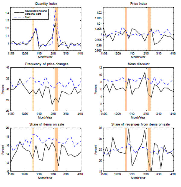
3.1.1 Overall impact on quantities and prices
Salient features of the strike's impact on retailing activities are presented in figure 1. As the top panel shows, stores whose employees were on strike experienced, on average, a staggering 50 percent drop in sales volumes over the conflict's duration. Some stores even saw sustained declines in quantities close to 80 percent. The drop was somewhat more pronounced in the first few weeks, suggesting that some shoppers who had initially declined to cross picket lines or to limit their purchases quickly returned. This modest rebound aside, the drop in revenues at establishments on strike was large and sustained for the duration of the labor conflict. News organizations reporting on the conflict indicated that shelves were generally fully stocked but that few shoppers were strolling the aisles. For this reason, we believe that supply constraints made a negligible contribution to the large drop in quantities observed at stores on strike. In sharp contrast, establishments in our group of stores that benefited from the strike witnessed large increases in revenues--over 30 percent, on average, with some stores even seeing their revenues more than double. Contrary to stores on strike, those that benefitted continued to have their regular employees present to serve consumers, replenish the shelves, and move products from warehouses to stores. In the absence of disruptions to their ability to supply products, the sudden rise in demand for these stores is thus unambiguously interpretable as a demand shock.
The top panel of figure 1 further suggests that a majority of consumers displaced by the strike returned to their previous shopping location at the end of the conflict: Sales volumes immediately rebounded at stores that had been on strike and fell sharply at stores that had benefited from the strike. The normalization was incomplete, however. In the year that followed the end of the conflict, sales volumes at stores that had been on strike were still 10 percent below sales volumes before the strike, whereas stores that had benefited from the strike retained some of the customers displaced by the strike. This fact could be consistent with theories that emphasize consumer loyalty to stores and chains such as switching costs (for example, Kleshchelski and Vincent, 2009).9 The immediate return of sales volumes toward their pre-conflict levels suggests that consumer preferences for points of purchase may persist even after consumers have switched stores for nearly five months. It is also possible that other factors were at play. For instance, stores with significantly higher sales volumes during the strike may have been able to offer fresher produce as a result. Such benefits may, in turn, have helped them retain consumers at the end of the conflict.
As the middle panel shows, price movements during the conflict, at only a couple of percentage points, were more than an order of magnitude smaller than swings in sales volumes, suggestive of a flat supply curve. For example, if we attribute the observed rise in prices at stores not on strike
entirely to a positive demand shock, then the estimates in table 4 imply a supply elasticity equal to
![]() . This modest estimate falls slightly if we control for inflation over the strike period by measuring the demand shock's effect as the
rise in excess of that for the price index of the full IRI sample.10 These supply elasticity estimates for the retail sector are markedly lower than the
0.18 figure reported by Shea (1993) for the U.S. manufacturing sector. One explanation for the difference could be that Shea's (1993) estimate applies to a one-year horizon whereas the
Southern California strike ended after five months, leaving less time for prices to adjust to higher demand. However, our evidence for the longer post-strike period, which features persistently large differences in demand and no supply disruptions at both groups of stores, also points to little if
any price response.11
. This modest estimate falls slightly if we control for inflation over the strike period by measuring the demand shock's effect as the
rise in excess of that for the price index of the full IRI sample.10 These supply elasticity estimates for the retail sector are markedly lower than the
0.18 figure reported by Shea (1993) for the U.S. manufacturing sector. One explanation for the difference could be that Shea's (1993) estimate applies to a one-year horizon whereas the
Southern California strike ended after five months, leaving less time for prices to adjust to higher demand. However, our evidence for the longer post-strike period, which features persistently large differences in demand and no supply disruptions at both groups of stores, also points to little if
any price response.11
It is also apparent that price movements were similar between stores on strike and stores not on strike before, during, and after the conflict. After rising a couple percent in the spring and summer of 2003, prices declined a little in the months prior to the strike, then rose over 3 percent in the first half of the conflict before retracing half of that rise in the second half. Overall, divergences in price movements between the two groups of stores were short-lived and not exceptionally large in comparison to other relative price movements over our sample period. After the strike, constraints on stores' ability to adjust prices and to supply goods vanished. Fair pricing motives that could have made retailers reluctant to boost prices amid exceptionally high demand would have greatly eased now that customers could shop freely at all stores. Despite some persistent differences in the quantity indexes, our price indexes show little economically meaningful divergence between the two groups of stores.
To provide a more direct comparison of the level of prices between stores that saw their demand soar and stores that saw their demand collapse, we next look at the cost of purchasing identical baskets of goods. We consider three such baskets. The first basket (the "fixed" basket) consists of all barcodes continuously available at both groups of stores over the two-year period displayed in figure 1, that is, over a period starting 26 weeks before and ending 78 weeks after the beginning of the conflict. The number of units purchased for each barcode is set to the average weekly number of units sold across all stores over the two-year period. This fixed-quantity basket is reasonably representative of overall purchases in Southern California, accounting for nearly 70 percent of total revenues over the period. At the product category level, the coverage of the basket ranges from 27 percent of total revenues for razors to 95 percent for peanut butter. The second basket (the "on-strike" basket) corresponds to the number of units purchased at stores on strike, again using only barcodes that are continuously available at both groups of stores. Similarly, the third basket (the " not-on-strike" basket) consists of the number of units sold at stores not on strike. Contrary to the fixed basket, the composition of the on-strike and not-on-strike baskets varies from week to week in line with shoppers' actual consumption.
The lower panel of figure 1 reports the cost of purchasing each of the three baskets at the mean transaction price observed at stores on strike relative to that at stores not on strike. (See the appendix for the exact formulas.) All three ratios tell the same story: The cost of purchasing any of our baskets at stores on strike relative to stores not on strike hovered near its pre-strike level for the duration of the conflict. A slight increase in the relative price of the baskets at stores that were on strike is apparent several months after the end of the conflict. We are reluctant to attribute this rise in the ratios to a price response to persistently lower demand given the historical variability of the sample.
We note that shoppers at stores on strike could have purchased identical baskets of goods for an equal or even lower price at stores that were not on strike at any point over our two-year period, a finding that suggest some insensitivity to the level of prices on the part of consumers. This conclusion comes with a number of caveats. Because the identity of stores and retail chains is censored, we cannot control for differences in factors such as income and sales taxes that may affect the level of prices across areas. Also, our baskets comprise solely barcodes that are simultaneously available in both groups of stores; by ignoring roughly 30 percent of store revenues in our product categories, we may be overlooking the effect of private labels on the effective costs of a typical basket. Finally, retailers sell items in product categories that are not covered by the IRI sample.
3.1.2 Price adjustments, price discounts, and the labor conflict
Figure 2 presents some key statistics on the broader pricing strategies of retailers before, during, and after the strike. The mean of each statistic over these periods is reported in table 4. On average, stores on strike saw their weekly frequency of posted price changes drop 4.3 percentage points during the conflict, with a reduction in regular price adjustments accounting for most of the drop. The fraction of items on sale (the middle-left panel of figure 2) declined 1.2 percentage point to 22.0 percent while the mean discount conditional on a sale (the middle-right panel) was unchanged. In short, stores on strike broadly managed to maintain the importance of sales during the conflict. Stores not on strike experienced a somewhat smaller drop in the frequency of posted price changes, 3.0 percentage points, that reflected small declines in both sales-related and regular price adjustments.
On the one hand, the continued use of sales by stores whose demand tumbled suggests that engaging in price discrimination is an important endeavor of retailers independently of their level of demand. Perhaps it also reflects a desire from stores on strike to project a business-as-usual image, or an implicit promise to offer bargain shoppers some opportunities to buy a portion of their basket at a discounted price every week. Indeed, it is conceivable that price-sensitive shoppers who continued to patronize stores on strike would have found it unfair to see their loyalty rewarded with higher prices. On the other hand, the reduction in regular price adjustments seems consistent with limited human resources hindering stores' ability to reprice. It is also possible that, given markedly lower sales volumes, stores on strike would have tolerated larger deviations of regular prices from their optimum because fixed repricing costs would have been spread over a smaller number of units sold.12 We also note that the level of individual prices continued to be coordinated within stores belonging to the same retail chain (the lower-right panel) despite variation across stores in the magnitude of the drop in demand and ability to use managerial staff to fill positions previously held by striking employees. In fact, the share of prices equal to the chain price edged up a couple of percentage points during the strike at both stores on strike and stores not on strike.
As noted above, stores on strike recouped only 4 out of every 5 dollars in lost business once the conflict ended. To win back customers, they increased the frequency and depth of sales in the ensuing year. The middle panels of figure 2 show that the share of discounted barcodes and the mean discount both rose a couple of percentage points before slowly edging back.13
To further explore the strategic use of sales during and after the conflict, we break down discounts into 10-percentage-point bins, starting with discounts that are below or equal to 10 percent, then below or equal to 20 percent but greater than 10 percent, and so on. Figure 3 displays the contribution of discounts in each bin to total revenues (the top row of panels) and to total savings (the lower row of panels).14 The upper-left panel shows that the contribution of items to total revenues generally was declining in the size of the discounts extended. Before the strike, discounts up to 10 percent accounted for almost 8 cents out of every dollar in revenues at stores that were subsequently affected by the conflict, while items offered at discounts in excess of 50 percent accounted for only about 2 cents out of every dollar in revenues. The lower-left panel shows that discounts in the 40 percent to 50 percent range, which were both substantial and frequent, allowed shoppers to lock in the largest savings. By contrast, very small and very large discounts contributed little to actual consumer savings because they were either too small or too infrequent to have a large impact. The distribution of contributions to total revenues and to total savings of discounts had similar shapes in the pre-conflict period at stores unaffected by the strike than at stores affected by the strike, although discounts of medium sizes played a somewhat lesser role in their overall marketing strategy.
During the strike, the number of items on sales declined only a little at affected stores during the strike. The upper-left panel of figure 2 shows that the importance of small and medium discounts for total revenues fell most while that of discounts in excess of 50 percent actually rose some. This shift toward deep discounts may have been part of a marketing strategy to lure shoppers to stores despite the strike, as heavy discounts make for good advertising. That said, the contribution to total savings of heavily discounted items was offset by the lesser importance of small and medium discounts, leaving the mean saving on the entire basket about unchanged. For stores that were not on strike, we also witness a decline in the importance of small and medium discounts during the conflict period but do not find a corresponding rise in the importance of very large discounts.
Once the strike was over, the contribution of small and medium discounts to total revenues and to total savings rose above its pre-strike level at both groups of stores. The importance of discounts in excess of 50 percent also rose at stores that had not been on strike, catching up with the similar increase documented at stores on strike during the conflict. In sum, the evidence is consistent with stores that had been on strike offering more frequent discounts--small, medium, and large--than usual to win back customers, and stores that had avoided the strike responding with more frequent sales of all sizes to retain them. Set against the background of differing swings in demand over the strike and the post-strike periods, these similarities in the recourse to sales suggest that retailers attach much value to matching changes in their local competitors' pricing strategies.
3.2 A shorter labor conflict: the 2003 St. Louis grocery strike and lockout
The 2003 St. Louis grocery strike and lockout paints a broadly similar portrait as the longer conflict in Southern California: Pricing strategies of stores on strike and stores not on strike broadly resembled each other despite highly diverging demand. It started on October 7 when employees at several supermarket chains went on strike or were locked-out after voting down a tentative labor agreement. The dispute ended 24 days later when negotiating teams reached an agreement that proved acceptable to all parties.
The main effects of the conflict on prices and quantities are shown in figure 4. Due to the smaller size of the St. Louis sample (22 stores compared to 107 stores in Southern California), we compare establishments whose revenues dropped more than 10 percent (generically referred to as "on strike") to all other establishments in the sample (generically referred to as "not on strike"). Picketing was again effective at deterring shopping activities, with stores on strike seeing sales volumes plunge about 45 percent, on average, while stores not on strike experienced a modest increase. Reading through the weekly volatility, prices at stores not on strike rose a touch more around the time of the conflict than prices at stores on strike. However, this slight divergence was part of a broader trend over the two-year period displayed and thus difficultly attributable to the strike. Moreover, price movements on a like-for-like basis were much more similar between the two groups of stores over the period displayed and around the strike in particular; our relative price measures controlling for the composition of the basket, which are shown at the bottom of figure 4 and employ the same methodology as those computed earlier for Southern California, were very stable.
Of note, sales volumes at stores on strike fully recovered as soon as the labor conflict was over, in contrast with the customer base erosion apparent at stores on strike in Southern California. Given limited household inventories, a 24-day conflict is arguably too long for customers unwilling to cross picket lines at their usual supermarket not to go shopping elsewhere. The recovery in sales volumes thus suggests some stickiness in consumer preferences for particular establishments that are not captured in standard models of store switching costs such as Kleshchelski and Vincent (2009), where store changes are permanent. In any case, the quick recovery in sales volumes probably explains why we did not observe a rise in the frequency and depth of discounts (shown in the middle panels of figure 5 and documented in table 5) in the wake of the St. Louis conflict.
4 Major weather events as exogenous demand shocks
Our next set of demand shocks were created by Mother Nature; their occurrence was unambiguously exogenous to retail activities in general and to supermarkets' pricing strategies in particular. We first look at Hurricane Katrina that, in the span of a few tragic weeks in the summer of 2005, led to massive population displacement. Stores located in areas that received an inflow of refugees experienced a sharp rise in store frequentation that persisted for well over a year. We then look at shopping sprees triggered by snowstorms and hurricanes. Contrary to strikes and Hurricane Katrina, these storms do not feature a reconfiguration of retailers' customer base but rather a temporary increase in the demand of all customers.
4.1 Hurricane Katrina
In August 2005, Hurricane Katrina created an estimated $108 billion in property damages (in 2005 dollars), making it the most expensive natural disaster in U.S. history. It was also directly responsible for the tragic loss of about 1,200 lives and the displacement of roughly 1 million persons.15 The city of New Orleans, Louisiana, sustained the most extensive damage due to the failure of its levee system, which led to the flooding of approximately 80 percent of the city. The flooding of residential areas made it impossible for many displaced households to return home for several months or years, and some households even chose to permanently relocate elsewhere. According to research conducted at the U.S. Census Bureau and reported in Geaghan (2011), as of late 2009, 31,500 households in the New Orleans metropolitan area (7 percent of the area's total) did not consider themselves permanently resettled.16
The hurricane had disruptive consequences on retail activities in New Orleans and other affected states. Of the 23 New Orleans stores that participated in the IRI sample on the eve of the tragedy, five exited the sample as soon as the storm hit while one store ceased to report data for a period of eight months. Similarly, five out of the nine stores in the Mississippi sample did not report data for a week or two around the hurricane. Although the IRI dataset contains no information that would permit us to ascertain that these sample exits and missing reports were caused by the hurricane, we interpret their coincidental timing as strongly suggestive that they were.
As figure 6 shows, the hurricane also affected retail activities at stores that remained in business. In the weeks and months that followed the disaster, stores that continued to report data to the IRI experienced sales volumes that were, on average, about 20 percent higher than before the disaster. We found an equally large rise in the smaller Mississippi sample (not shown); a smaller effect is also apparent for the Houston, Texas, sample (also not shown). We interpret this persistent rise in sales volumes at continuing stores as evidence that mass relocation boosted the demand for supermarket products in some areas that were relatively unaffected by the storm. Supporting our interpretation is the fact that, according to Geaghan (2011), 74 percent of displaced New Orleans householders reported living with an acquaintance.17 In addition, the persistent increase in sales volumes of food products as well as housekeeping and personal care products, which are shown separately in figure 6, were of a similar proportion, consistent with mass relocation boosting the demand of supermarkets' entire product offering. Indeed, we observe increases in all 29 product categories in the sample. The upper-left panel of figure 6 also features a short-lived but outsized 60 -percent surge in sales volumes of housekeeping supplies and personal care products the precise week that Hurricane Katrina hit. Revenues from product categories such as toothbrushes and razors witnessed transitory increases in excess of 100 percent, again consistent with population displacement being a key driver of retail activities over the period.
Our empirical evidence provides little if any support to the view that retailers took advantage of higher demand brought about by the hurricane to raise prices, either initially when spending on personal care products skyrocketed or over the medium run when store frequentation was boosted by mass relocation. The upper-right panel of figure 6 shows that the price of food products and of personal care and housekeeping products both rose in the weeks that followed the storm before erasing some of these gains. When we average over the period covered by the federal emergency declaration, we find that prices were 1.4 percent higher overall than they were over the 26 -week period before the hurricane. As table 6 reports, this increase is modestly larger than the average rise across IRI markets not directly affected by Hurricane Katrina (that is, excluding New Orleans, Mississippi, and Houston). Muted price movements translate into small estimates of the short-term elasticity of supply. If we measure the price impact as the rise in the New Orleans price index in excess of the average rise for IRI markets not directly affected by Hurricane Katrina, then our estimate of the (short-run) elasticity of supply is 0.03 .
When we compute the elasticity of supply using price and quantity movements over the longer period after the federal emergency relative to the pre-storm period, we get a supply elasticity estimate of 0.13 . However, we are reluctant to interpret this medium-run estimate as suggestive that retailers took advantage of higher demand to boost prices for two main reasons. First, this estimate may be biased upward by hurricane-related disruptions to the region's food supply. Second, price pressure was not broad based, as the price of housekeeping and personal care products rose in line with the national average.
The remaining panels of figure 6 provide further results regarding the impact of the hurricane on retailers' broader pricing strategy. The frequency of price changes edged down during the federal emergency period, and reverted to its pre-hurricane average
for about a year before sliding in the fall of 2006. The hurricane had a somewhat more apparent effect on the mean discount, which temporarily slid from between 5 and ![]() percent of the regular price in the weeks before the hurricane to a low near 2 percent,
before rebounding at the end of the federal emergency declaration. Much of this decline reflects a lower proportion of items on sales, especially in late September and early October, rather than a shift in customer spending toward items with lesser or no discounts, as hinted by the relative
stability of both the mean discount and the share of items on sale in the first couple weeks after the storm.
percent of the regular price in the weeks before the hurricane to a low near 2 percent,
before rebounding at the end of the federal emergency declaration. Much of this decline reflects a lower proportion of items on sales, especially in late September and early October, rather than a shift in customer spending toward items with lesser or no discounts, as hinted by the relative
stability of both the mean discount and the share of items on sale in the first couple weeks after the storm.
4.2 Major snowstorms and hurricanes
Major weather events such as large snowstorms and hurricanes can affect the demand for supermarket products through several channels. Storms that result in the closing of schools and workplaces force households to consume a greater proportion of their meals at home, thus boosting demand for food items. Similarly, the demand for personal care and housekeeping products may rise as households engage in greater home production or take advantage of their trip to the supermarket to purchase items other than food. Storms may also displace consumption across time periods by making it difficult or impossible to shop on certain days. In particular, some households may seek to build their domestic inventories in anticipation of a storm to ensure continued supplies, while others may need to replenish their inventories once the storm is over.
4.2.1 Identification
We have identified 59 combinations of an IRI market and a major snow episode whose disruptive consequences were favorable to the triggering of a shopping spree. Many of these combinations feature a peak in average store revenues of 10 percent or more relative to the previous few weeks. While there were hundreds of smaller snowstorms in our sample, we expressly choose to leave them aside because storms whose disruptive effects last only a couple of days are less likely to leave a clear imprint in supermarket data collected weekly.
In identifying disruptive snowstorm episodes, we account for the fact that some localities have a greater ability to cope with snowfall than others. Snow accumulations that have crippling effects in Southern states, where snowstorms are scarce and snow plowing equipment is in short supply, may have only limited disruptive effects in Northern states, where local authorities are accustomed to clearing snow off the streets rapidly. To do so, we match our IRI scanner data with the U.S. National Oceanic and Atmospheric Administration's Regional Snowfall Index (RSI) and the Federal Emergency Management Agency's (FEMA) list of federal disaster declarations. The RSI controls for differences in historical snow precipitation and the authorities' ability to cope with snow through the setting of precipitation thresholds that are specific to nine U.S. regions (the West Coast of the United States is not covered due to insufficiently frequent snowstorms). Storms whose social impact is roughly in the top half of historical storms in their region are given a rank between 1 and 5. Many of the snow episodes in our sample were ranked "3-major," "4-crippling," or "5-exceptional," placing them in the top 5 percent of storms in terms of regional-level disruptiveness. Many storms were also granted an "emergency" or a "disaster relief" status by FEMA because they were of "such severity and magnitude that effective response [was] beyond the capabilities of the State and the local governments and that Federal assistance [was] necessary."18
We validate our list of snow episodes against daily snowfall measurements reported by local weather stations to avoid situations in which a disruptive storm at the regional level results in little snow accumulation or passes as rain in a particular market. We also use local daily snowfall measurements to include a number of storms that likely had large localized effects but whose regional impact, as measured by the RSI, was small. In a few cases, our snow episodes cover two snowstorms rather than one because the separate meteorological systems are indistinguishable in weekly data. Finally, we incorporate a few major snowstorms from the U.S. West Coast for which RSI scores are not available. The list of snowstorms, along with their cumulative snowfall, RIS classification, and FEMA declaration, is provided in an online appendix.
We follow a similar strategy for identifying hurricanes that are likely to induce shopping sprees. We look at all " emergency" and "major disaster" declarations by FEMA that are attributed to a hurricane. We then validate our list against daily rainfall and maximum wind speed measurements from local weather stations.19 In total, we have identified 21 combinations of an IRI market and a hurricane, which we also list in our online appendix along with their characteristics.
4.2.2 Illustration: 2009-2010 winter in Washington, D.C.
Figure 7 illustrates some effects of major storms on retail activities using two snow episodes that hit Washington, D.C., during the 2009-2010 winter. The first episode began on Friday, December 18, 2009, and left 41.7 centimeters (16.4 inches) of snow at D.C.'s Reagan National Airport. Federal offices were closed the following Monday and operated on an unscheduled leave basis for two more days due to impracticable roads in parts of the metropolitan area. The second snow episode was more disruptive, consisting of two back-to-back blizzards that together blanketed the U.S. capital with 72.6 centimeters (28.6 inches) of snow. Federal offices closed early as the first blizzard moved in on Friday, February 5, 2010, remained closed through February 12, and then operated on an unscheduled leave basis through February 16. As is typical of the episodes in our sample, the National Weather Service and local media began reporting on the approaching snowstorms several days ahead of their occurrence.
The upper-left panel of figure 7 shows that sales volumes peaked 20 to 45 percent above their trend in the December 2009 and February 2010 snow episodes. The timing of the surge in quantities differs between the two episodes, although the use of weekly retail data limits our ability to identify their timing precisely (note that IRI weeks run from Monday to Sunday). As is apparent for both episodes, the quantity of food products and of personal care and housekeeping products spiked around the storms, supporting our treatment of major snowstorms as shocks to the overall demand of supermarkets rather than as shocks specific to some product categories. In the first episode, quantities of both groups of products rose 10 percent in the week of the storm relative to their recent trend, and rose even more in the ensuing week. In the second episode, sales volumes surged 27 percent for personal care and housekeeping products in the week encompassing the beginning of the second episode and 45 percent for food products. The demand for food products remained above its recent trend during the ensuing week. The large impact of the second storm may be due to the anticipation of greater snow totals (and, if our experience is representative, it could also reflect some learning from the first episode that shopping in advance of the storm avoids some headaches).
The two snowstorm episodes left no apparent imprint on price indexes, as shown in the upper-right panel. Similarly, the frequency of price changes, the mean discount, the share of items on sales, and the share of store revenues derived from items on sales were all within the range experienced over the 2009-2010 winter. Our econometric analysis below, on the broader sample of snowstorms and hurricanes, confirms these impressions.
4.2.3 Econometric analysis
There is some uncertainty regarding the precise timing of when weekly retail activities should feel the effects of storms most strongly. Storms that hit early in the week or whose disruptive effects are anticipated may affect retail activities prior to the storm. Similarly, storms that hit late
in the week or that require domestic inventory rebuilding by households afterwards could have some effect in the week after the storm. As a first step into our investigation, we ignore this timing issue and compare various retailing statistics in the week corresponding to the observed peak in
quantities to their respective average in the weeks prior to the storm. More precisely, for a storm beginning in week ![]() , we identify the peak in quantity over the weeks
, we identify the peak in quantity over the weeks ![]() ,
, ![]() , and
, and ![]() and then compare the statistic of interest for that peak week by its average over the weeks
and then compare the statistic of interest for that peak week by its average over the weeks ![]() to
to ![]() (the " pre-storm period").20
(the " pre-storm period").20
Our sample of snow episodes supports the patterns apparent in figure 7, namely that major snowstorms boost consumer spending on supermarket items while having little if any influence on pricing. The mean peak in quantities around snowstorms is 12.9 percent higher than the average over the pre-storm period, whereas the peak in prices is only 0.1 percent higher. A simple statistical test that the population mean of the ratio across snow episodes equals 1 is rejected for quantities but not for prices. The peak quantity and price responses, as well as their statistical significance, are nearly identical for hurricanes. For both types of storms, we also find similar statistics on broader features of our stores' pricing strategies between the week of the peak in quantities and the pre-storm period. This remarkable finding suggests that retailers broadly retain their usual pricing strategies.
We next follow a regression-based approach similar to that used by Chevalier, Kashyap, and Rossi (2003) in their study of demand peaks around holidays. We regress our statistics of interest (illustrated here with the log of our market-specific price index) on a quadratic time trend and a set of
dummies marking the week immediately before (
![]() ), the week during (
), the week during (
![]() ), and the week after (
), and the week after (
![]() ) a storm,
) a storm,
Table 7 reports the results for our key statistics of interest. For major snowstorms, we find that the boost to quantities occurs almost entirely in the week of the storm. We also observe a statistically-significant small decline in quantities of about 1.9 percent in the week after the storm. This decline is suggestive that greater shopping activities during snowstorms result in the bringing forward of some household expenditures, leading to a small pull back in the week immediately after. The corresponding estimates for prices point to a small increase during the week of the storm that is not statistically significant. In the case of hurricanes, we find a statistically significant boost to spending in both the week immediately before and the week of the storm. This finding suggests that hurricanes primarily pull forward consumption expenditures, perhaps due to a greater predictability of these events and a greater risk that households could experience reduced supplies for a protracted period. A pull back is also observed in the week immediately after a hurricane, although it is not statistically significant at standard confidence levels.
4.2.4 Discussion
Our analysis suggests that supermarkets do not take advantage of transitory peaks in demand brought about by major snowstorms and hurricanes to boost prices. More broadly, they appear to implement pricing strategies during and around storms that are highly similar to those in other periods. In this sense, the response to peaks in demand brought about by storms differs from the finding that prices tend to fall during periods of peak demand around holidays (see Warner and Barsky (1995), MacDonald (2000), and Chevalier, Kashyap, and Rossi (2003)). This difference could reflect a number of factors. Notably, whereas the timing of holidays is perfectly predictable, the occurrence of a major snowstorm or hurricane can be anticipated at most a week or so in advance and only with great uncertainty. This limited predictability may not leave enough time for manufacturers to adjust production or for retailers to alter their pricing strategy; circulars may already have been printed and, in any case, there can be lags of several months in the planning of sales and promotions (see Anderson et al. (2013) for a discussion). Moreover, one cannot exclude that fair pricing motives of the kind described by Rotemberg (2005, 2011) could be at play. Retailers may want to avoid being perceived as unjustly profiting off their customers' unusually high marginal utility for fear of losing their business in the future. That said, our sample excludes products whose consumption is essential during storms, such as de-icing salt, batteries, and snow shovels. Our sample instead contains products consumed year-round and for which several brands are typically available. A retailer that would want to take advantage of temporarily high demand would thus have to raise effective prices over a broad product offering. This feat could be achieved by reducing the number or depth of sales rather than by raising regular prices but our sample does not contain support for this channel.
5 Conclusion
We have shown that the level of supermarket prices responds little to large swings in demand brought about by labor conflicts, mass population relocation, and shopping sprees around storms and hurricanes. This evidence is consistent with flat short- to medium-term supply curves in the retail sector. In particular, it seems inconsistent with the marginal cost of retailers being sensitive to the level of demand because of fixed factors of production, a hypothesis that is often made in macro models. And when prices did fluctuate some, we have found that variations in the frequency and depth of sales were often important channels of price adjustment, thus cautioning against focusing solely on regular prices to understand the transmission of shocks.
A number of authors have reported that, contrary to the textbook treatment, prices tend to fall in periods of peak demand, including for the kind of goods present in our sample. On the surface, this evidence seems supportive of models featuring countercyclical markups. However, the absence of a price response to major snowstorms and hurricanes suggests that the perfect predictability of holidays and the passing of seasons make their associated peaks in demand of a very different nature than those triggered by shocks that are difficult to forecast. In addition, if retailers respond little to demand shocks, they seem concerned with keeping up with the pricing strategies of their local competitors. This fact is most clearly seen from price movements during and after the labor conflicts in our sample, when retailers with radically different demand shocks nonetheless tracked their local competitors' pricing movements and recourse to sales and promotions.
These observations invite a reconsideration of the place occupied by the retail sector in macro models. Many modelers conflate the notion of producers and retailers, and then calibrate their model to match pricing facts of retailers only. Our analysis suggests that the retail sectors' short- to medium-term supply curve is quite flat relative to that of other sectors such as manufacturing, a finding in line with the relatively low-margin, high-volume nature of the industry. Although we do not observe (marginal) costs in our dataset, it seems sensible to conjecture that our low supply elasticity estimates could reflect relatively steady marginal costs and markups, a possibility more directly suggested by Eichenbaum, Jaimovich, and Rebelo's (2011) evidence that item-level retail markups vary little around their mean. If so, then investigations of markup behavior and deviations from constant returns to scale at lower levels of the production chain seem much needed.
References
[1] Anderson, Eric, Emi Nakamura, Duncan Simester, and Jón Steinsson, (2013). "Informational Rigidities and the Stickiness of Temporary Sales," NBER Working Papers 19350, National Bureau of Economic Research, Inc.
[2] Angrist, Joshua D. and Guido W. Imbens (1995). "Two-Stage Least Squares Estimation of the Average Causal Effects in Models with Variable Treatment Intensity," Journal of the American Statistical Association, vol. 90(430), pages 431-442.
[3] Barro, Robert, (1972). "A Theory of Monopolistic Price Adjustment," Review of Economic Studies, vol. 39(1), pages 17-26.
[4] Bernanke, Ben, Jean Boivin, and Piotr S. Eliasz, (2005). "Measuring the Effects of Monetary Policy: A Factor-augmented Vector Autoregressive (FAVAR) Approach," Quarterly Journal of Economics, vol. 120(1), pages 387-422.
[5] Bils, Mark and Peter J. Klenow, (2004). "Some Evidence on the Importance of Sticky Prices," Journal of Political Economy, vol. 112(5), pages 947-985.
[6] Blake, Eric S. and Ethan J. Gibney, (2011). "The Deadliest, Costliest, and Most Intense United States Tropical Cyclones from 1851 to 2010 (and Other Frequently Requested Hurricane Facts)," NOAA Technical Memorandum NWS NHC-6, U.S. National Oceanic and Atmospheric Administration.
[7] Bradley, Ralph, (2012). "Price Index Estimation Using Price Imputation for Unsold Items," chapter in: Scanner Data and Price Indexes, NBER Studies in Income and Wealth, vol. 64, pages 349-382, University of Chicago Press.
[8] Bronnenberg, Bart J., Michael W. Kruger, and Carl F. Mela, (2008). "Database Paper: The IRI Marketing Data Set," Marketing Science, vol. 27(4), pages 745-748.
[9] Cavallo, Alberto, Eduardo Cavallo, and Roberto Rigobon (2013). "Prices and Supply Disruptions during Natural Disasters," NBER Working Papers, 19474, National Bureau of Economic Research, Inc.
[10] Chevalier, Judith A. and Anil K. Kashyap (2013). "Best Prices: Price Discrimination and Consumer Substitution," NBER Working Papers, 1668 0, National Bureau of Economic Research, Inc.
[11] Chevalier, Judith A., Anil K. Kashyap, and Peter E. Rossi, (2003). "Why Don't Prices Rise During Periods of Peak Demand? Evidence from Scanner Data," American Economic Review, vol. 93(1), pages 15-37.
[12] Christiano, Lawrence J., Martin Eichenbaum, and Charles L. Evans, (1999) . "Monetary policy shocks: What have we learned and to what end?," Handbook of Macroeconomics, in: John B. Taylor and Michael Woodford (ed.), vol. 1, pages 65-148, Elsevier.
[13] Cleveland, William P. and Stuart Scott, (2007), "Seasonal Adjustment of Weekly Time Series with Application to Unemployment Insurance Claims and Steel Production," Journal of Official Statistics, vol. 23, pages 209-221.
[14] Coibion, Olivier, Yuriy Gorodnichenko, and Gee Hee Hong, (2012). "The Cyclicality of Sales, Regular and Effective Prices: Business Cycle and Policy Implications," NBER Working Papers 18273, National Bureau of Economic Research, Inc.
[15] Dhyne, Emmanuel, Luis J. Álvarez, Hervé Le Bihan, Giovanni Veronese, Daniel Dias, Johannes Hoffmann, Nicole Jonker, Patrick Lünnemann, Fabio Rumler, and Jouko Vilmunen, (2005). " Price Setting in the Euro Area: Some Stylized Facts from Individual Consumer Price Data," Working Paper 524, European Central Bank.
[16] Eichenbaum, Martin, Nir Jaimovich, and Sergio Rebelo (2011). "Reference Prices, Costs, and Nominal Rigidities," American Economic Review, vol. 101(1), pages 234-62.
[17] Federal Emergency Management Agency, "Declared Disasters by Year or State," last accessed December 2, 2011, http://www.fema.gov/news/disaster_totals_annual.fema.
[18] Gagnon, Etienne, David López-Salido, and Nicolas Vincent, (2013). "Individual Price Adjustment along the Extensive Margin," chapter in: NBER Macroeconomics Annual 2012, vol. 27, pages 235-281.
[19] Geaghan, Kimberly A., (2011). "Forced to Move: An Analysis of Hurricane Katrina Movers 2009 American Housing Survey: New Orleans," Social, Economic, and Housing Statistics Division Working Paper Number 2011-17, U.S. Census Bureau.
[20] Golosov, Mikhail and Robert E. Lucas Jr., (2007). "Menu Costs and Phillips Curves," Journal of Political Economy, vol. 115, pages 171-199.
[21] Gopinath, Gita and Oleg Itskhoki, (2010). "Frequency of Price Adjustment and Pass-Through," Quarterly Journal of Economics, vol. 125 (2), pages 675-727.
[22] Hall, Robert E., (2009). "By How Much Does GDP Rise If the Government Buys More Output?," Brookings Papers on Economic Activity, vol. 40(2), pages 183-249.
[23] Hong, Gee Hee and Nicholas Li, (2013). " Market Structure and Cost Pass-Through in Retail," Working Papers tecipa-470, University of Toronto, Department of Economics.
[24] Karadi, Peter and Adam Reiff (2012)."Large shocks in menu cost models," Working Paper Series, 1453, European Central Bank.
[25] Klenow, Peter J. and Oleksiy Kryvtsov, (2008). "State-Dependent or Time-Dependent Pricing: Does It Matter for Recent U.S. Inflation?," Quarterly Journal of Economics, vol. 123(3), pages 863-904.
[26] Kleshchelski, Isaac and Nicolas Vincent (2009). "Market Share and Price Rigidity," Journal of Monetary Economics, vol. 56(3), pages 344-352.
[27] Kruger, Michael W. and Daniel Pagni, (2008). IRI Academic Data Set Description, version 1.31, Chicago: Information Resources Incorporated.
[28] Lach, Saul, (2007). "Immigration and Prices," Journal of Political Economy, vol. 115(4), pages 548-587.
[29] Liu, Zheng and Sylvain Leduc, (2013)." Uncertainty Shocks Are Aggregate Demand Shocks," 2013 Meeting Papers 270, Society for Economic Dynamics.
[30] Lee, Lung-Fei and Mark M. Pitt, (1986). "Microeconometric Demand Systems with Binding Nonnegativity Constraints: The Dual Approach," Econometrica, Econometric Society, vol. 54(5), pages 1237-1242.
[31] MacDonald, James M., (2000). "Demand, Information, and Competition: Why Do Food Prices Fall at Seasonal Demand Peaks?," Journal of Industrial Economics, vol. 48(1), pages 27-45.
[32] Nakamura, Emi, (2008). "Pass-Through in Retail and Wholesale," American Economic Review: Papers & Proceedings, vol. 98(2), pages 430-437.
[33] Nakamura, Emi and Jón Steinsson (2008). "Five Facts about Prices: A Reevaluation of Menu Cost Models," Quarterly Journal of Economics, vol. 123(4), pages, 1415-1464.
[34] National Climate Data Center, "NCDC Climate Data Online: Daily Surface Data," last accessed December 5, 2011, http://cdo.ncdc.noaa.gov/pls/plclimprod/somdmain.somdwrapper.
[35] Ravn, Morten, Stephanie Schmitt-Grohé, and Martín Uribe, (2006). "Deep Habits," Review of Economic Studies, Oxford University Press, vol. 73(1), pages 195-218.
[36] Romer, Christina D. and David H. Romer (2004)."A New Measure of Monetary Shocks: Derivation and Implications," American Economic Review, vol. 94(4), pages, 1055-1084.
[37] Rotemberg, Julio J., (2005). " Customer anger at price increases, changes in the frequency of price adjustment and monetary policy," Journal of Monetary Economics, vol. 52(4), pages 829-852.
[38] Rotemberg, Julio J., (2011). "Fair Pricing," Journal of the European Economic Association, vol. 9(5), pages 952-981.
[39] Shea, John, (1993). "Do Supply Curves Slope Up?," Quarterly Journal of Economics, vol. 108(1), pages 1-32.
[40] Warner, Elizabeth J. and Robert B. Barsky, (1995). "The Timing and Magnitude of Retail Store Markdowns: Evidence from Weekends and Holidays," Quarterly Journal of Economics, vol. 110(2), pages 321-352.
A.1 Data trimming and filtering
We perform a number of data cleaning steps to create a sample suitable for our purposes. We only use observations pertaining to grocery stores to ensure maximum comparability across stores and retail chains. The IRI sample also includes observations from drugstores but the number of such stores is more limited than for grocery stores. We exclude two product categories from the sample, cigarettes and photo supplies, because their prices and advertising are heavily regulated and they gradually became obsolete over our sample period, respectively. As is common with scanner data, we obtain a weekly transaction price by dividing total revenue by the number of units sold. In a tiny proportion of cases, the division yields a price with fractional cents (e.g., $4.8573). For New York City, fractional prices represent less than 0.2 percent of posted prices. The origin of these fractional prices is unclear; they may be related to reporting errors, price adjustments during the week, membership card usage, etc. Upon inspection, we opted to keep them in the sample as they were very close to prices in neighboring periods. Excluding them would be inconsequential for our results.
In addition to analyzing posted prices, we consider measures of regular prices and reference prices to capture lower-frequency movements in prices. Our regular price filter is based on that proposed by Nakamura and Steinsson (2008) in section A of their technical appendix. It removes temporary
price drops that are followed by an increase to a price at or above the previous price or to a new regular price. Our implementation uses the parameters ![]() ,
, ![]() , and
, and ![]() .21 Our reference price filter is a variant of that of Eichenbaum, Jaimovich, and Rebelo (2011). The reference price of an item in week
.21 Our reference price filter is a variant of that of Eichenbaum, Jaimovich, and Rebelo (2011). The reference price of an item in week ![]() corresponds to the modal price observed over a 13 -week centered window.
corresponds to the modal price observed over a 13 -week centered window.
To compute monthly posted, regular, and reference price statistics, we retain only weekly observations that encompass the 15th day of each month to match the BLS' practice of sampling in the same narrow time window every month. Finally, all weekly and monthly statistics employ only observations from frequently traded items that are free of anomalous price movements, as we now detail in the context of deriving price and quantity indexes.
A.2 Constructing indexes of total revenues, prices, and quantities
We first compute indexes of total store revenues at the IRI market-product category level (the "stratum" level). This task is made possible by the IRI dataset's comprehensive coverage of items available for sale at participating stores within each of the 29 product categories. This feature
makes it possible to track the evolution of a store's total revenues by product category over time and to monitor the entry and exit of items in its offering. Occasionally, all observations from a store may be coded as missing. In such problematic weeks, we impute missing store's total revenues
using average revenue growth for the subset of stores in the same IRI market whose revenues for the product category are observed. Formally, let ![]() index stores in market
index stores in market ![]() and product category
and product category ![]() that are present in the sample at week
that are present in the sample at week ![]() and for which total sales in week
and for which total sales in week ![]() are known (because they were either directly observed or imputed from the
preceding period). Let also
are known (because they were either directly observed or imputed from the
preceding period). Let also
![]() be an indicator that store
be an indicator that store ![]() ' data are not systematically missing in
the period. Whenever all observations are missing at some stores, we first compute the revenue growth for stores that are reporting correctly in period
' data are not systematically missing in
the period. Whenever all observations are missing at some stores, we first compute the revenue growth for stores that are reporting correctly in period ![]() ,
,
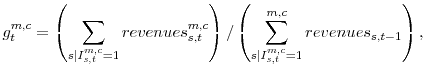
We follow a methodology similar to that employed by the BLS for the U.S. CPI to compute disaggregated price indexes for the IRI sample. We first obtain an estimate of inflation at the IRI market-product category level using a geometric mean formula,
We transform our inflation estimates at the stratum into measures of the price level by calculating these estimates' cumulative product over time. We then scale the price indexes so that their geometric mean equals unity in 2005. We finally obtain a real same-store quantity index at the stratum level by deflating our total revenue index by our geomeans price indexes.23 This approach of computing a quantity index by effectively pooling price and spending data from separate surveys mimics that employed by the BEA for disaggregated real personal consumption expenditures in the U.S. National Income and Product Accounts.
Also echoing the BEA methodology, we aggregate stratum statistics across product categories using a chain-weighted approach. We compute a Fisher quantity index,
![]() , as the geometric average of a Paasche quantity index,
, as the geometric average of a Paasche quantity index,
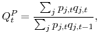
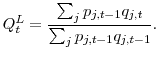
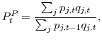
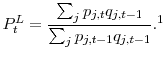
A.3 Comparing the level of prices
One attractive feature of the IRI sample is that we observe item barcodes, which allows us to directly compare the level of prices across stores for specific items or for baskets of items. Let
![]() be a set of items sold simultaneously in stores
be a set of items sold simultaneously in stores ![]() and
and ![]() in period
in period ![]() . Let
. Let
![]() be the number of units of item
be the number of units of item ![]() in the comparison basket.24 The price of purchasing the basket in store
in the comparison basket.24 The price of purchasing the basket in store ![]() relative to the price of purchasing it in store
relative to the price of purchasing it in store
![]() is given by
is given by
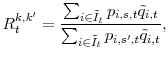
A.4 Adjustments for breaks and seasonal patterns
Several IRI product categories display a jump in the number of barcodes per store at the beginning of 2007. The origin of this jump is not explicated in IRI documentation but it likely reflects a broadening of product category definitions rather than an actual increase in the number of barcodes offered by stores. To prevent spurious breaks in our disaggregated total sales and quantity indexes, we impute total sales growth in the problematic week at the stratum level using average total sales growth of items that are present in both the last week of 2006 and the first week of 2007.25 In addition, a number of stores exiting the IRI sample early report exceptionally large sales--sometimes over ten times normal volumes--during their last couple of weeks in the sample. The reason for such skyrocketing reported sales is unclear to us but their occurrence seems largely orthogonal to the object of our study. For this reason, we systematically drop the last two periods in the sample of stores that exit early to remove any associated breaks in the level of our series.
In addition to controlling for breaks, we often want to control for seasonal variation and holidays when comparing retailing activities during, say, natural disasters, to those during periods in which they are absent. To this end, we filter our stratum-level indexes with a procedure developed by
Cleveland and Scott (2007) for weekly time series. The filter allows us to account for the precise timing of holidays and to exclude particular periods from the computation of the seasonal factors. Our analysis of labor conflicts excludes the strike periods while that of Hurricane Katrina drops the
week immediately before the storm and the entire federal disaster declaration period. For shopping sprees around major snowstorms and hurricanes, we exclude the weeks immediately before, during, and after the storms. National aggregates use all weekly observations. Price and quantity indexes use
multiplicative seasonal factors whereas all other indicators, which are in percent, use additive factors.
Table 1: Posted price adjustments statistics
| Product Category | Mean Weekly Observations | Mean Weekly Sales | Weekly Statistics (in percent): Frequency | Weekly Statistics (in percent): Share decreases | Weekly Statistics (in percent): Mean increase | Weekly Statistics (in percent): Mean decrease | Monthly Statistics (in percent): Frequency | Monthly Statistics (in percent): Share decreases | Monthly Statistics (in percent): Mean increase | Monthly Statistics (in percent): Mean decrease |
|---|---|---|---|---|---|---|---|---|---|---|
| Beer | 196259 | 10346913 | 21.6 | 47.4 | 8.2 | 8.6 | 36.9 | 46.7 | 9.5 | 9.9 |
| Blades | 46388 | 817634 | 17.7 | 47.7 | 18.5 | 20.9 | 31.6 | 45.6 | 17.8 | 21.3 |
| Carbonated Beverages | 360592 | 15307421 | 43.9 | 49.2 | 20.0 | 20.5 | 51.3 | 48.1 | 19.5 | 20.3 |
| Coffee | 155122 | 3609792 | 25.1 | 48.3 | 16.9 | 18.2 | 42.2 | 46.5 | 17.3 | 18.9 |
| Cold Cereal | 274289 | 8381493 | 28.8 | 48.0 | 23.0 | 25.1 | 43.8 | 47.6 | 24.6 | 27.4 |
| Condiments | 64706 | 980701 | 17.8 | 47.8 | 14.7 | 15.9 | 36.6 | 49.9 | 23.5 | 25.2 |
| Deodorant | 138584 | 862847 | 21.4 | 50.0 | 24.0 | 25.2 | 41.4 | 50.7 | 12.1 | 12.9 |
| Diapers | 58779 | 1642245 | 27.7 | 50.2 | 12.3 | 12.8 | 44.3 | 48.8 | 18.8 | 20.4 |
| Facial Tissue | 35411 | 1133320 | 30.4 | 49.4 | 17.3 | 18.2 | 52.8 | 49.4 | 23.6 | 24.7 |
| Frozen Dinner | 387087 | 6781188 | 36.6 | 49.2 | 23.2 | 24.0 | 55.2 | 49.2 | 21.4 | 22.4 |
| Frozen Pizza | 131892 | 3676668 | 40.6 | 49.0 | 21.3 | 22.1 | 34.8 | 48.3 | 17.4 | 19.5 |
| Hot Dogs | 52276 | 2105301 | 36.8 | 48.1 | 27.1 | 28.8 | 47.1 | 46.8 | 25.5 | 28.2 |
| Household Cleaners | 82487 | 969090 | 18.8 | 48.8 | 15.8 | 17.4 | 43.9 | 49.1 | 19.9 | 21.3 |
| Laudry Detergent | 111344 | 3666854 | 29.7 | 48.8 | 19.7 | 21.1 | 42.8 | 45.7 | 19.7 | 22.2 |
| Margarine/Butter | 68568 | 1644178 | 26.4 | 47.5 | 18.3 | 20.0 | 34.3 | 42.7 | 17.5 | 21.3 |
| Mayonnaise | 47705 | 1410940 | 22.1 | 46.1 | 18.4 | 21.0 | 41.2 | 45.6 | 11.3 | 12.9 |
| Milk | 113946 | 13607991 | 26.1 | 47.2 | 10.2 | 11.4 | 31.0 | 46.2 | 16.5 | 18.7 |
| Paper Towels | 40895 | 2664537 | 27.3 | 48.5 | 15.4 | 16.6 | 40.8 | 47.7 | 17.1 | 18.7 |
| Peanut Butter | 49848 | 1180936 | 23.6 | 47.6 | 13.8 | 14.9 | 39.1 | 46.9 | 16.0 | 17.6 |
| Razors | 7444 | 112878 | 23.1 | 49.1 | 16.8 | 18.3 | 38.5 | 48.5 | 16.7 | 19.2 |
| Salty Snack | 364220 | 9506203 | 30.2 | 48.8 | 19.8 | 20.7 | 42.1 | 48.3 | 20.6 | 21.5 |
| Shampoo | 132957 | 976285 | 23.8 | 50.0 | 21.6 | 22.7 | 40.4 | 50.0 | 21.3 | 22.9 |
| Soup | 316460 | 4448335 | 23.7 | 47.9 | 23.2 | 25.1 | 37.9 | 47.1 | 23.7 | 26.2 |
| Spaghetti Sauce | 131143 | 2068199 | 29.0 | 49.0 | 20.6 | 21.6 | 46.3 | 48.6 | 21.8 | 23.1 |
| Sugar Substitutes | 26218 | 438704 | 13.7 | 48.0 | 10.1 | 11.5 | 27.5 | 46.4 | 12.0 | 14.1 |
| Toilet Tissue | 53117 | 4067906 | 32.6 | 48.2 | 15.1 | 16.2 | 46.1 | 47.4 | 16.9 | 18.3 |
| Tooth Brushes | 69569 | 519586 | 22.4 | 49.8 | 24.7 | 26.1 | 36.3 | 50.1 | 26.1 | 28.1 |
| Tooth Paste | 111224 | 1114115 | 23.8 | 49.5 | 21.8 | 23.0 | 38.6 | 49.4 | 22.7 | 24.2 |
| Yogurt | 246642 | 4940942 | 34.2 | 49.5 | 19.4 | 19.8 | 46.7 | 49.0 | 19.7 | 20.7 |
| Total | 3875174 | 108983204 | n.a. | n.a. | n.a. | n.a. | n.a. | n.a. | n.a. | n.a. |
| Mean | 133627 | 3758042 | 26.9 | 48.6 | 18.3 | 19.6 | 41.1 | 47.8 | 19.0 | 20.8 |
| Weighted Mean | n.a. | n.a. | 30.4 | 48.4 | 17.6 | 18.7 | 42.3 | 47.6 | 18.7 | 20.3 |
Table 2: Regular price adjustments statistics
| Product Category | Mean Weekly Observations | Mean Weekly Sales | Weekly Statistics (in percent): Frequency | Weekly Statistics (in percent): Share decreases | Weekly Statistics (in percent): Mean increase | Weekly Statistics (in percent): Mean decrease | Monthly Statistics (in percent): Frequency | Monthly Statistics (in percent): Share decreases | Monthly Statistics (in percent): Mean increase | Monthly Statistics (in percent): Mean decrease |
|---|---|---|---|---|---|---|---|---|---|---|
| Beer | 196259 | 10346913 | 9.3 | 46.4 | 6.6 | 7.3 | 21.2 | 44.6 | 8.1 | 8.7 |
| Blades | 46388 | 817634 | 5.9 | 47.7 | 10.5 | 17.5 | 16.4 | 42.5 | 11.6 | 18.0 |
| Carbonated Beverages | 360592 | 15307421 | 18.6 | 49.2 | 16.1 | 17.2 | 32.0 | 47.4 | 16.6 | 17.9 |
| Coffee | 155122 | 3609792 | 9.9 | 47.1 | 11.3 | 14.2 | 24.8 | 44.1 | 13.0 | 15.3 |
| Cold Cereal | 274289 | 8381493 | 9.3 | 46.6 | 13.0 | 17.6 | 21.1 | 44.9 | 14.8 | 20.0 |
| Condiments | 64706 | 980701 | 7.2 | 46.5 | 10.9 | 13.5 | 18.3 | 43.9 | 13.3 | 16.5 |
| Deodorant | 138584 | 862847 | 5.6 | 57.5 | 15.0 | 22.3 | 15.6 | 52.0 | 16.6 | 22.3 |
| Diapers | 58779 | 1642245 | 8.5 | 55.8 | 8.4 | 11.1 | 21.0 | 53.5 | 9.2 | 11.2 |
| Facial Tissue | 35411 | 1133320 | 10.8 | 49.9 | 11.9 | 14.6 | 23.4 | 47.9 | 14.3 | 17.2 |
| Frozen Dinner | 387087 | 6781188 | 10.7 | 50.1 | 15.1 | 18.2 | 24.7 | 49.2 | 16.7 | 20.0 |
| Frozen Pizza | 131892 | 3676668 | 13.0 | 49.3 | 14.8 | 17.3 | 27.6 | 48.5 | 16.4 | 18.9 |
| Hot Dogs | 52276 | 2105301 | 10.2 | 44.9 | 16.3 | 20.5 | 15.7 | 46.9 | 12.9 | 17.7 |
| Household Cleaners | 82487 | 969090 | 6.0 | 48.9 | 10.9 | 15.5 | 21.6 | 42.2 | 16.8 | 21.9 |
| Laudry Detergent | 111344 | 3666854 | 9.5 | 50.5 | 12.6 | 16.1 | 22.2 | 49.4 | 13.8 | 16.9 |
| Margarine/Butter | 68568 | 1644178 | 9.1 | 43.2 | 10.8 | 13.9 | 21.6 | 40.6 | 12.9 | 16.1 |
| Mayonnaise | 47705 | 1410940 | 8.8 | 41.7 | 10.8 | 14.9 | 20.5 | 37.8 | 11.9 | 16.4 |
| Milk | 113946 | 13607991 | 12.1 | 44.9 | 6.7 | 8.5 | 26.1 | 42.9 | 7.8 | 9.8 |
| Paper Towels | 40895 | 2664537 | 10.1 | 48.7 | 10.1 | 12.9 | 22.3 | 46.4 | 12.3 | 15.2 |
| Peanut Butter | 49848 | 1180936 | 9.6 | 45.2 | 9.5 | 11.3 | 21.4 | 44.2 | 11.2 | 13.3 |
| Razors | 7444 | 112878 | 7.5 | 56.4 | 11.5 | 17.5 | 20.3 | 50.6 | 13.0 | 18.2 |
| Salty Snack | 364220 | 9506203 | 10.3 | 49.5 | 14.7 | 16.9 | 19.8 | 47.3 | 16.2 | 18.7 |
| Shampoo | 132957 | 976285 | 6.6 | 58.0 | 14.3 | 20.3 | 18.1 | 52.9 | 15.5 | 20.4 |
| Soup | 316460 | 4448335 | 8.2 | 46.7 | 13.9 | 17.8 | 20.3 | 44.8 | 15.6 | 19.6 |
| Spaghetti Sauce | 131143 | 2068199 | 9.6 | 48.3 | 13.1 | 15.8 | 23.2 | 46.9 | 14.9 | 17.6 |
| Sugar Substitutes | 26218 | 438704 | 4.7 | 46.2 | 7.4 | 11.4 | 13.2 | 43.1 | 9.4 | 13.6 |
| Toilet Tissue | 53117 | 4067906 | 13.5 | 47.8 | 10.1 | 12.1 | 26.3 | 45.9 | 12.1 | 14.3 |
| Tooth Brushes | 69569 | 519586 | 7.8 | 54.8 | 18.7 | 23.2 | 17.2 | 52.3 | 20.8 | 25.7 |
| Tooth Paste | 111224 | 1114115 | 6.4 | 52.4 | 14.0 | 19.2 | 16.7 | 49.6 | 15.9 | 20.5 |
| Yogurt | 246642 | 4940942 | 9.3 | 49.6 | 12.1 | 14.3 | 21.0 | 48.0 | 13.1 | 15.4 |
| Total | 3875174 | 108983204 | n.a. | n.a. | n.a. | n.a. | n.a. | n.a. | n.a. | n.a. |
| Mean | 133627 | 3758042 | 9.2 | 49.1 | 12.1 | 15.6 | 21.2 | 46.6 | 13.7 | 17.1 |
| Weighted Mean | n.a. | n.a. | 11.2 | 48.0 | 12.0 | 14.5 | 23.7 | 46.1 | 13.3 | 16.0 |
Table 3: Basic chain prices statisics
| Product Category | Posted Prices: Adjustement probability (in percent) Equal to chain price (in percent) | Posted Prices: Adjustement probability (in percent) Unconditional | Posted Prices: Adjustement probability (in percent) Conditional on chain price change | Posted Prices: Adjustement probability (in percent) Conditional on no chain price change | Regular Prices: Adjustement probability (in percent) Equal to chain price (in percent) | Regular Prices: Adjustement probability (in percent) Unconditional | Regular Prices: Adjustement probability (in percent) Conditional on chain price change | Regular Prices: Adjustement probability (in percent) Conditional on no chain price change |
|---|---|---|---|---|---|---|---|---|
| Beer | 66.6 | 24.9 | 73.0 | 10.3 | 67.3 | 12.0 | 49.2 | 6.2 |
| Blades | 77.0 | 18.6 | 70.6 | 9.2 | 76.1 | 9.8 | 39.7 | 4.1 |
| Carbonated Beverages | 65.8 | 42.8 | 90.0 | 17.4 | 68.6 | 17.6 | 67.9 | 11.4 |
| Coffee | 71.5 | 25.1 | 79.4 | 11.9 | 72.3 | 11.9 | 54.1 | 6.2 |
| Cold Cereal | 68.1 | 27.2 | 83.7 | 11.8 | 72.0 | 9.7 | 57.9 | 5.4 |
| Condiments | 78.6 | 24.1 | 73.8 | 10.2 | 74.5 | 11.2 | 30.9 | 4.1 |
| Deodorant | 76.1 | 27.8 | 78.4 | 13.7 | 75.5 | 11.0 | 43.1 | 6.2 |
| Diapers | 70.0 | 27.4 | 84.4 | 13.2 | 73.1 | 10.4 | 60.5 | 6.3 |
| Facial Tissue | 72.8 | 34.6 | 86.5 | 13.6 | 74.8 | 10.7 | 55.1 | 6.4 |
| Frozen Dinner | 71.3 | 37.5 | 87.7 | 17.6 | 74.4 | 11.9 | 58.4 | 8.3 |
| Frozen Pizza | 74.4 | 19.2 | 72.8 | 9.3 | 75.5 | 8.8 | 44.4 | 3.7 |
| Hot Dogs | 72.6 | 35.5 | 90.5 | 13.1 | 79.5 | 9.3 | 69.5 | 5.8 |
| Household Cleaners | 72.0 | 29.1 | 81.9 | 13.0 | 73.5 | 10.5 | 49.0 | 6.3 |
| Laudry Detergent | 71.3 | 24.6 | 84.0 | 9.3 | 74.2 | 9.3 | 63.2 | 4.2 |
| Margarine/Butter | 70.2 | 21.0 | 79.9 | 8.7 | 72.5 | 9.6 | 58.2 | 4.6 |
| Mayonnaise | 67.6 | 25.1 | 81.6 | 11.6 | 70.4 | 13.3 | 64.8 | 6.1 |
| Milk | 72.3 | 17.9 | 74.7 | 8.9 | 74.0 | 9.1 | 53.6 | 4.1 |
| Paper Towels | 71.2 | 23.7 | 83.2 | 11.9 | 74.6 | 9.5 | 61.4 | 5.6 |
| Peanut Butter | 69.1 | 22.4 | 78.9 | 10.7 | 71.1 | 10.7 | 57.1 | 5.3 |
| Razors | 77.1 | 26.5 | 75.4 | 12.7 | 73.5 | 13.0 | 34.0 | 5.9 |
| Salty Snack | 76.4 | 29.5 | 89.6 | 12.4 | 81.4 | 10.0 | 67.5 | 6.3 |
| Shampoo | 79.9 | 25.4 | 77.0 | 10.8 | 77.1 | 10.3 | 35.5 | 4.5 |
| Soup | 72.2 | 22.9 | 79.8 | 9.7 | 74.4 | 9.6 | 54.7 | 4.4 |
| Spaghetti Sauce | 72.2 | 27.9 | 83.1 | 11.8 | 73.9 | 10.2 | 55.3 | 5.6 |
| Sugar Substitutes | 73.8 | 14.0 | 67.0 | 7.0 | 75.2 | 7.4 | 44.9 | 2.7 |
| Toilet Tissue | 65.8 | 29.2 | 85.2 | 13.7 | 69.5 | 12.9 | 65.3 | 7.3 |
| Tooth Brushes | 70.2 | 28.2 | 78.0 | 16.1 | 68.7 | 16.0 | 48.7 | 8.6 |
| Tooth Paste | 77.8 | 24.6 | 78.6 | 11.1 | 77.0 | 9.2 | 40.4 | 4.5 |
| Yogurt | 72.6 | 32.3 | 87.5 | 12.0 | 76.9 | 8.8 | 61.5 | 5.1 |
| Mean | 72.4 | 26.5 | 80.6 | 11.8 | 73.8 | 10.8 | 53.3 | 5.7 |
| Weighted Mean | 71.2 | 28.4 | 82.3 | 12.3 | 73.2 | 11.3 | 58.0 | 6.4 |
| Observations | n.a. | 1193827794 | 838593893 | 355233901 | n.a. | 1193827794 | 1058562164 | 135265593 |
Table 4: Mean Statistics before during and after the 2003-2004 Southern California supermarket strike
| statistic | On Strike: Before | On Strike: During | On Strike: After | Not on Strike: Before | Not on Strike: During | Not on Strike: After |
|---|---|---|---|---|---|---|
| Quantity index | 1.000 | 0.513 | 0.904 | 1.000 | 1.336 | 1.036 |
| Quantity index: std. deviation | (0.004) | (0.020) | (0.004) | (0.005) | (0.018) | (0.006) |
| Price index | 1.000 | 1.013 | 1.012 | 1.000 | 1.021 | 1.009 |
| Price index: std. deviation | (0.002) | (0.003) | (0.001) | (0.002) | (0.002) | (0.001) |
| Frequency of posted price changes | 45.9 | 41.6 | 48.1 | 34.1 | 31.1 | 32.5 |
| Frequency of posted price changes: std. deviation | (0.4) | (0.6) | (0.3) | (0.3) | (0.4) | (0.3) |
| Frequency of regular price changes | 20.0 | 16.1 | 19.4 | 15.2 | 13.4 | 12.7 |
| Frequency of regular price changes: std. deviations | (0.3) | (0.4) | (0.3) | (0.2) | (0.3) | (0.2) |
| Share of items on sale | 23.2 | 22.0 | 25.0 | 18.1 | 16.8 | 18.9 |
| Share of items: std. deviations | (0.3) | (0.5) | (0.2) | (0.2) | (0.3) | (0.2) |
| Mean discount | 9.4 | 9.4 | 10.2 | 8.3 | 6.8 | 8.5 |
| Mean discount: std. deviations | (0.1) | (0.2) | (0.2) | (0.1) | (0.2) | (0.1) |
| Share of revenues from items on sale | 30.4 | 28.2 | 31.4 | 27.3 | 24.2 | 28.1 |
| Share of revenues from items on sale: std. deviation | (0.4) | (0.7) | (0.3) | (0.4) | (0.4) | (0.3) |
| Share of prices equal to chain price | 53.2 | 55.8 | 51.9 | 59.9 | 62.4 | 63.5 |
| Share of prices equal to chain price: std. deviation | (0.4) | (0.5) | (0.3) | (0.3) | (0.3) | (0.2) |
| Addendum: Price index IRI sample ex. striking markets | 1.000 | 1.004 | 1.019 | 1.000 | 1.004 | 1.019 |
Table 5: Mean Statistics before during and after the 2003 St. Louis supermarket strike
| Statistic | On Strike:Before | On Strike: During | On Strike: After | Not on Strike: Before | Not on Strike: During | Not on Strike: After |
|---|---|---|---|---|---|---|
| Quantity index | 1.001 | 0.566 | 0.967 | 1.002 | 1.053 | 0.939 |
| Quantity index: std. deviation | (0.007) | (0.060) | (0.004) | (0.011) | (0.022) | (0.008) |
| Price index | 1.000 | 1.001 | 1.005 | 1.000 | 1.011 | 1.032 |
| Price index: std. deviation | (0.001) | (0.002) | (0.001) | (0.001) | (0.001) | (0.001) |
| Frequency of posted price changes | 24.7 | 22.5 | 24.9 | 22.6 | 21.1 | 22.6 |
| Frequency of posted price changes: std. deviation | (0.3) | (3.1) | (0.2) | (0.3) | (0.8) | (0.2) |
| Frequency of regular price changes | 6.3 | 5.6 | 6.5 | 5.6 | 3.9 | 5.1 |
| Frequency of regular: std. deviation | (0.3) | (1.4) | (0.2) | (0.3) | (0.3) | (0.1) |
| Share of items on sale | 19.7 | 17.9 | 19.5 | 17.8 | 18.4 | 18.2 |
| Share of items on sale: std. deviation | (0.2) | (0.5) | (0.1) | (0.3) | (0.1) | (0.2) |
| Mean discount | 9.7 | 9.1 | 10.3 | 9.6 | 10.8 | 10.8 |
| Mean discount: std. deviation | (0.2) | (0.5) | (0.1) | (0.1) | (0.4) | (0.1) |
| Share of revenues from items on sale | 28.5 | 23.5 | 28.8 | 26.5 | 28.3 | 28.1 |
| Share of revenues from items on sale: std. deviation | (0.4) | (0.9) | (0.2) | (0.4) | (0.5) | (0.3) |
| Share of prices equal to chain price | 94.3 | 92.7 | 94.0 | 87.5 | 87.3 | 87.7 |
| Share of prices equal to chain price: std. deviation | (0.2) | (1.1) | (0.2) | (0.4) | (0.4) | (0.3) |
| Addendum: Price index IRI sample ex. striking markets | 1.000 | 1.001 | 1.017 | 1.000 | 1.001 | 1.017 |
Table 6: Mean statistics before during and after 2005 Hurricane Katrina in New Orleans Louisiana
| statistic | All: Before | All: During | All: After | Food: Before | Food: During | Food: After | Housekeeping and Personal Care: Before | Housekeeping and Personal Care: During | Housekeeping and Personal Care: After |
|---|---|---|---|---|---|---|---|---|---|
| Quantity index | 1.001 | 1.220 | 1.135 | 1.001 | 1.224 | 1.136 | 1.001 | 1.188 | 1.131 |
| Quantity index: std. deviation | (0.008) | (0.019) | (0.009) | (0.008) | (0.021) | (0.010) | (0.010) | (0.049) | (0.007) |
| Price index | 1.000 | 1.014 | 1.030 | 1.000 | 1.015 | 1.031 | 1.000 | 1.004 | 1.025 |
| Price index: std. deviation | (0.001) | (0.002) | (0.002) | (0.001) | (0.002) | (0.002) | (0.002) | (0.003) | (0.003) |
| Frequency of posted price changes | 30.6 | 28.9 | 30.0 | 30.9 | 29.4 | 30.3 | 28.7 | 25.6 | 28.4 |
| Frequency of posted price changes: std. deviaton | (0.3) | (0.5) | (0.3) | (0.4) | (0.6) | (0.3) | (0.6) | (0.8) | (0.5) |
| Mean discount | 5.2 | 3.9 | 5.0 | 4.9 | 4.0 | 4.8 | 7.2 | 3.2 | 6.6 |
| Mean discount: std. deviation | (0.1) | (0.3) | (0.1) | (0.1) | (0.4) | (0.1) | (0.4) | (0.5) | (0.2) |
| Share of items on sale | 14.1 | 13.4 | 14.1 | 14.1 | 13.6 | 13.9 | 13.7 | 11.3 | 15.5 |
| Share of items on sale: std. deviation | (0.3) | (0.6) | (0.1) | (0.3) | (0.6) | (0.2) | (0.4) | (0.8) | (0.3) |
| Share of revenues from items on sale | 18.1 | 15.7 | 17.4 | 17.6 | 15.8 | 16.6 | 21.9 | 15.2 | 22.9 |
| Share of revenues from items on sale: std. deviation | (0.4) | (1.0) | (0.2) | (0.4) | (1.1) | (0.2) | (0.8) | (1.3) | (0.5) |
| Addendum: Price index IRI sample ex. Katrina areas | 1.000 | 1.007 | 1.017 | 1.000 | 1.007 | 1.016 | 1.000 | 1.007 | 1.026 |
| Addendum: Price index matched BLS sample | 1.000 | 1.008 | 1.013 | 1.000 | 1.007 | 1.008 | 1.000 | 1.010 | 1.033 |
Table 7: Effect of major snowstorms and hurricanes on retailing activities
| Quantity index (in logs*100) | Price index (in logs*100) | Frequency of price changes (percent) | Frequency of regular price changes (percent) | Mean discount (percent) | Share of items on sale (percent) | Share of revenues from items on sale (percent) | Share of prices equal to chain price (percent) | |
|---|---|---|---|---|---|---|---|---|
| Major snowstorms: Quantity peak analysis: Pre-storm average | 0.00E+00 | 0.00E+00 | 31.96 | 10.77 | 8.91 | 16.97 | 26.86 | 70.02 |
| Major snowstorms: Quantity peak analysis:Peak week value | 12.88 | 1.20E-01 | 31.53 | 10.30 | 8.46 | 16.85 | 25.93 | 70.15 |
| Major snowstorms: Quantity peak analysis: t-test of zero difference | 14.14 | 1.51E+00 | -1.36 | -2.70 | -3.46 | -0.68 | -3.11 | 0.37 |
| Major snowstorms: Regression results:Estimated coefficients : Week before storm | 0.74 | 0.09 | -0.64 | -0.2 | -0.17 | -0.29 | -0.47 | 0.29 |
| Major snowstorms: Regression results:Estimated coefficients : Week before storm (t-statistics) | (1.47) | (1.85) | (-2.81 ) | (-1.52 ) | (-1.51 ) | (-1.86 ) | (-1.92 ) | (1.09 ) |
| Major snowstorms: Regression results:Estimated coefficients : Week during storm | 11.70 | 0.00 | -0.33 | -0.49 | -0.32 | -0.03 | -0.73 | 0.22 |
| Major snowstorms: Regression results:Estimated coefficients : Week during storm (t-statistics) | (23.36 ) | (-0.02 ) | (-1.47 ) | (-3.69 ) | (-2.88 ) | (-0.17 ) | (-3.04 ) | (0.84 ) |
| Major snowstorms: Regression results:Estimated coefficients: Week after storm | -1.85 | 0.07 | -0.61 | -0.44 | -0.26 | -0.36 | -0.91 | 0.38 |
| Major snowstorms: Regression results:Estimated coefficients: Week after storm (t-statistics) | (-3.69 ) | (1.28 ) | (-2.69 ) | (-3.27 ) | (-2.34 ) | (-2.29 ) | (-3.78 ) | (1.42 ) |
| p-value joint significance | 0.00 | 0.20 | 0.00 | 0.00 | 0.00 | 0.05 | 0.00 | 0.33 |
| Number of snowstorms | 59 | 59 | 59 | 59 | 59 | 59 | 59 | 50 |
| Observations | 1456 | 1456 | 1456 | 1456 | 1456 | 1456 | 1456 | 1213 |
| Hurricanes: Quantity peak analysis: Pre-storm average | 0.00E+00 | 0.00E+00 | 30.19 | 11.05 | 7.22 | 15.73 | 24.08 | 72.91 |
| Hurricanes: Quantity peak analysis: Peak week value | 12.84 | 0.06 | 30.64 | 11.60 | 7.22 | 16.10 | 24.54 | 71.84 |
| Hurricanes: Quantity peak analysis: t-test of zero difference | 9.14 | 0.45 | 0.97 | 1.22 | 0.01 | 1.35 | 1.18 | -2.33 |
| Hurricanes: Regression results: Estimated coefficients : Week before hurricane | 6.44 | -0.18 | -0.2 | 0.41 | 0.09 | -0.1 | -0.35 | -0.12 |
| Hurricanes: Regression results: Estimated coefficients : Week before hurricane (t-statistics) | (7.36 ) | (-2.31 ) | (-0.55 ) | (1.68 ) | (0.49 ) | (-0.44 ) | (-0.91 ) | (-0.29 ) |
| Hurricanes: Regression results: Estimated coefficients : Week during hurricane | 6.03 | 0.13 | 0.71 | 0.82 | -0.34 | -0.34 | -0.64 | -1.02 |
| Hurricanes: Regression results: Estimated coefficients : Week during hurricane (t-statistics) | (6.90 ) | (1.67 ) | (1.96 ) | (3.33 ) | (-2.59 ) | (-1.50 ) | (-1.66 ) | (-2.60 ) |
| Hurricanes: Regression results: Estimated coefficients : Week after hurricane | -0.97 | 0.09 | 0.99 | 1.05 | -0.39 | -0.39 | -1.38 | -0.17 |
| Hurricanes: Regression results: Estimated coefficients : Week after hurricane (t-statistics) | (-1.11 ) | (1.17 ) | (2.72 ) | (4.29 ) | (-2.24 ) | (-1.71 ) | (-3.61 ) | (-0.43 ) |
| p-value joint significance | 0.00 | 0.01 | 0.01 | 0.00 | 0.01 | 0.20 | 0.00 | 0.08 |
| Number of hurricanes | 21 | 21 | 21 | 21 | 21 | 21 | 21 | 14 |
| Observations | 476 | 476 | 476 | 476 | 476 | 476 | 476 | 300 |
Figure 1: Impact of 2003 Southern California supermarket strike on quantities and prices
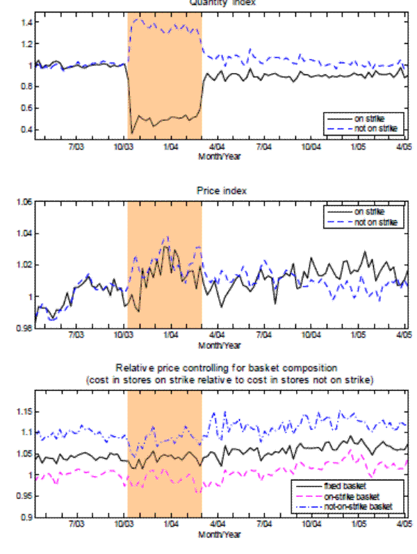 Figure 1 Data
Figure 2: Some key pricing features of the 2003 Southern California supermarket strike
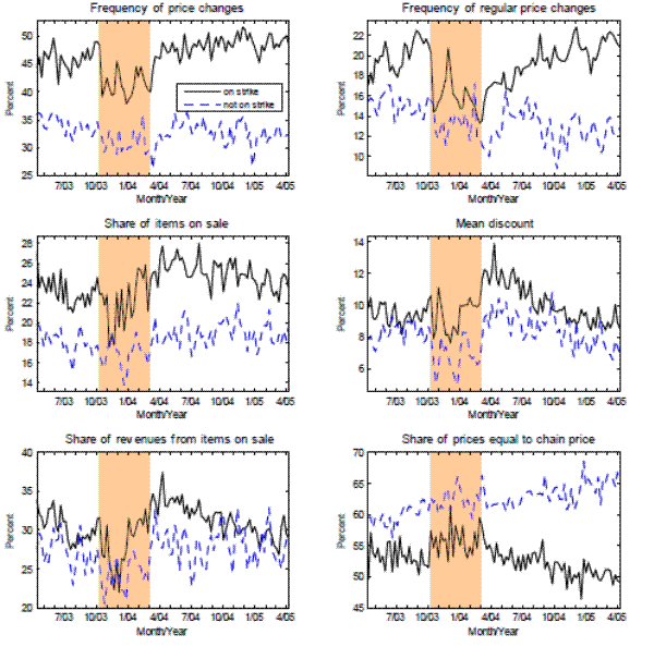 Figure 2 Data
Figure 3: Importance of discounts before, during, and after the 2003 Southern California supermarket strike
 Figure 3 Data
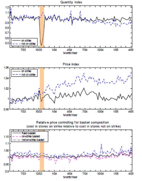
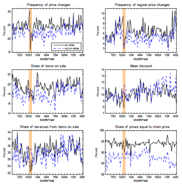
Figure 6: Impact of 2005 Hurricane Katrina on pricing decisions in New Orleans, Louisiana
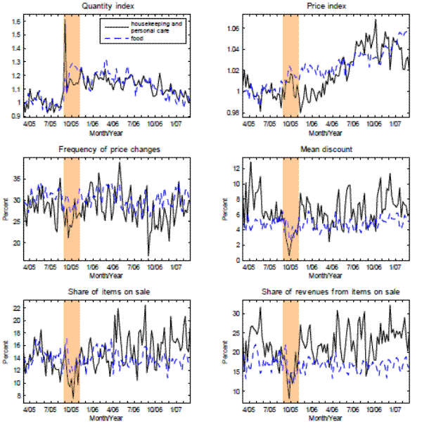 Figure 6 Data