
Board of Governors of the Federal Reserve System
International Finance Discussion Papers
Number 873, August 2006 --- Screen Reader Version*
Monetary Policy, Oil Shocks, and TFP: Accounting for the Decline in U.S. Volatility*
NOTE: International Finance Discussion Papers are preliminary materials circulated to stimulate discussion and critical comment. References in publications to International Finance Discussion Papers (other than an acknowledgment that the writer has had access to unpublished material) should be cleared with the author or authors. Recent IFDPs are available on the Web at http://www.federalreserve.gov/pubs/ifdp/. This paper can be downloaded without charge from the Social Science Research Network electronic library at http://www.ssrn.com/.
Abstract:
An equilibrium model is used to assess the quantitative importance of monetary policy for the post-1984 decline in U.S. inflation and output volatility. The principal finding is that monetary policy played a substantial role in reducing inflation volatility, but a small role in reducing real output volatility. The model attributes much of the decline in real output volatility to smaller TFP shocks. We also investigate the pattern of output and inflation volatility under an optimal monetary policy counterfactual. We find that real output volatility would have been somewhat lower, and inflation volatility substantially lower, had monetary policy been set optimally.
Keywords: Business cycles, optimal monetary policy
JEL Classification: E32, E31, E52
*We thank an anonymous referree, Shaghil Ahmed, Satyajit Chatterjee, Sanjay Chugh, Luca Dedola, Mike Dotsey, James Hamilton, John Leahey, Frank Schorfheide and seminar participants at the 2003 Society for Economic
Dynamics meetings and the 2005 Econometric Society meetings for their comments. We also thank John Fernald for
kindly providing us with his measure of TFP calculated with Susanto Basu and Miles Kimball. The views in this
paper are solely the responsibility of the authors and should not be interpreted as reflecting the views of the Board of
Governors of the Federal Reserve System, of the Federal Reserve Bank of Philadelphia, or of any other person
associated with the Federal Reserve System. Return to text
†Corresponding Author: Keith Sill, Research Department, Federal Reserve Bank of Philadelphia, Philadelphia, PA
19106, USA; Telephone: 215-574-3815; Fax: 215-574-4364; E-mail: [email protected] Return to text
1 Introduction
The volatility of the U.S. economy since the mid-1980s is much lower than it was during the prior 20-year period. The proximate causes of the increased stability and their relative importance remain unsettled, but the sharpness of the volatility decline and its timing has led authors such as Taylor (2000) to argue that a sudden shift in monetary policy is a prime candidate. Many studies in the economic volatility literature date the break in real output growth volatility around 1984, some four years after the beginning of the Volcker chairmanship of the FOMC.1 A growing body of research indicates that systematic monetary policy changed significantly with the onset of the Volcker chairmanship. For example, Gali et al. (2003) examine the Fed's systematic response to technology shocks and its implication for hours, output, and inflation. They find significant differences in the Fed's response pre-1979 and post-1979, and that post-1979 policy is close to optimal.
Has monetary policy played a quantitatively significant role in the volatility decline? Recent work by Boivin and Giannoni (2003) argues yes: their estimated structural models imply a reduced effect of monetary policy shocks in the post-1980 period that is almost entirely explained by an increase in the Fed's responsiveness to inflation and output. Their estimates suggest that the monetary transmission mechanism was different pre-1979 compared to post-1979, with most of the difference traced to a change in the monetary policy rule rather than to a change in private-sector behavior. On the other hand, the VAR analysis in Stock and Watson (2002), Stock and Watson (2003), Ahmed et al. (2004), and Primiceri (2003) indicates that monetary policy played little role in the moderation of output volatility, though it perhaps played a role in lowering the volatility of inflation.2 These studies tend to indicate that smaller shocks hitting the economy are the principal cause of the moderation in U.S. volatility.3
Standard models suggest that, aside from monetary policy, a change in the volatility of TFP may have played a significant role in the increased stability of the U.S. economy. Indeed, recent work by Arias et al. (2006) supports this view. Another plausible candidate for the less-volatile economy is a change in the magnitude and frequency of oil shocks. To assess the relative contributions of shocks and monetary policy to the decline in U.S. economic volatility we build a standard, sticky-price monetary model of the business cycle. The model is simulated over the high-volatility period 1956-1979 and the low-volatility period 1984-1999. The simulations use measured historical TFP, oil shocks, and monetary policy rules. Counterfactual analysis is used to quantify the relative contributions of TFP and oil shocks as well as monetary policy to the decline in output and inflation volatility since 1984.
Our principal finding is that while the change in monetary policy played a role in the postwar moderation of output volatility, most of the decline can be attributed to a reduction in the volatility of TFP and oil shocks. Our benchmark specification suggests that the change in monetary policy accounted for about 17 percent of the fall in output volatility, which is in line with the VAR evidence in Stock and Watson (2002). In contrast, we do find that monetary policy played a relatively more important role in stabilizing inflation, accounting for about 30 percent of the decline in its volatility.
A natural question that arises in our analysis is how the post-war pattern of volatility might have differed had monetary policy been set optimally. This paper is one of the first to investigate the implications of optimal monetary policy in a sticky-price model with endogenous capital accumulation.4 In the counterfactual optimal monetary policy specification, real output volatility would have been significantly lower, and inflation volatility dramatically lower, than what was observed in the postwar data. We find that output volatility would have been 20 to 30 percent lower over the postwar period and inflation volatility would have been nil, had policy been set according to the Ramsey plan.
The paper is organized as follows. Section 2 describes some facts about the recent volatility decline for the U.S. economy. Section 3 presents the model; section 4 describes the optimal monetary policy problem; and sections 5 and 6 discuss calibration and simulation results. Section 7 concludes.
2 Volatility Facts
The facts we wish to account for are the volatility patterns of output and inflation for the postwar U.S. economy. Table 1 shows the standard deviations of quarterly real GDP growth and GDP deflator inflation by decades, as well as for samples with breakpoints in 1979Q4 and 1984Q1.
What stands out for both output growth and inflation volatility are the low values of the 1990s, both of which are about half the level achieved in the 1970s and 1980s. Several studies have identified a breakpoint in real output growth volatility around 1984Q1. The table shows, using that break date, output growth volatility dropped by about half in the post-1984Q1 sample. For the standard deviation of inflation, the 1984 break date implies a dramatic decline on the order of 0.45 percentage points. If the sample is split at 1979Q3, corresponding to a commonly determined monetary policy break date, inflation volatility is seen to decline a more modest 0.13 percentage points. Clearly though, inflation volatility in the 1990s was a good bit lower than over the preceding decades.
As an alternative way of looking at the data, we show time-series plots for rolling standard deviations of HP-filtered real GDP and HP-filtered GDP deflator inflation in Figures 1 and 2. For real GDP, a large drop in volatility occurs in the early 1980s. A similar drop in volatility occurs for inflation, though inflation volatility was also low prior to its run-up in the 1970s.
The volatility of real GDP growth dropped almost 50 percent, and inflation volatility dropped about 30 percent. The way in which the early 1980s recessions are included in the subsamples has implications for the magnitude of calculated volatility. In the analysis below, we follow the literature that puts the volatility break date at the first quarter of 1984, which occurs about four years after the shift in monetary policy regime.
3 Model
The baseline model framework is a standard sticky-price business-cycle model similar to that in Ireland (2001). To investigate the contribution of oil shocks to economic volatility, we append an energy sector to the model so that energy use is tied to capital utilization as in Finn (1995).
The economy consists of a representative household,
representative finished-goods-producing firm, a continuum of
intermediate goods-producing firms indexed by i
![]() [0,1], and a central
bank. Time is discrete and is indexed by t = 0,1, 2...
Each producer of intermediate goods produces a distinct good,
indexed by i. The structure is symmetric, so the
intermediate goods sector can be modeled as a representative firm
that produces a generic intermediate good i.
[0,1], and a central
bank. Time is discrete and is indexed by t = 0,1, 2...
Each producer of intermediate goods produces a distinct good,
indexed by i. The structure is symmetric, so the
intermediate goods sector can be modeled as a representative firm
that produces a generic intermediate good i.
To generate interest-elastic money demand, we assume a cash-good
credit-good economy as in Lucas and Stokey (1987). The
representative household has preferences over consumption sequences
of cash goods ![]() , and
credit goods
, and
credit goods ![]() , and
hours worked
, and
hours worked ![]() :
:
![$\displaystyle E_{0}\sum\limits_{t=0}^{\infty}\beta^{t}[ \alpha_{1} \ln( c_{1,t}-b c_{1,t-1}) +\alpha_{2} \ln( c_{2,t}-b c_{2,t-1}) +\alpha\ln( 1-h_{t}) ]$](img5.gif)
where we allow for the possibility of habit persistence. Households must use cash held in advance to finance cash-good purchases. Consequently, they face the cash-in-advance constraint:
The household earns labor income
![]() , invests in
capital
, invests in
capital ![]() that it
rents to intermediate-goods-producing firms at rental rate
that it
rents to intermediate-goods-producing firms at rental rate
![]() and receives
a nominal dividend
and receives
a nominal dividend ![]() from the firms that it owns. It also gets a lump-sum transfer
from the firms that it owns. It also gets a lump-sum transfer
![]() from the central
bank. The household's budget constraint is:
from the central
bank. The household's budget constraint is:
The household chooses
![]() and
and ![]() to maximize equation (3.1) subject to the cash-in-advance
constraint, equation (3.2)
and the budget constraint equation (3.3).5 Let
to maximize equation (3.1) subject to the cash-in-advance
constraint, equation (3.2)
and the budget constraint equation (3.3).5 Let ![]() be the multiplier on the household's budget
constraint and
be the multiplier on the household's budget
constraint and
![]() be the
multiplier on the cash-in-advance constraint. Define
be the
multiplier on the cash-in-advance constraint. Define
![]() , and
, and
![]() The first-order conditions
for the household optimization problem are:
The first-order conditions
for the household optimization problem are:
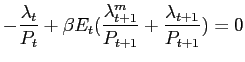
Equation (3.4) characterizes the household choice for cash good consumption, equation (3.5) characterizes the choice for credit good consumption, equation (3.6) characterizes the choice of labor effort, equation (3.7) characterizes the choice of money holdings, and equation (3.8) characterizes the choice for investment.
The representative finished-goods producing firm produces output
![]() using as inputs
the output
using as inputs
the output ![]() of
each intermediate goods producing firm. Each input is purchased at
price
of
each intermediate goods producing firm. Each input is purchased at
price ![]() . The
technology for producing the final good is given by:
. The
technology for producing the final good is given by:
![$\displaystyle y_{t}={\left[ \int_{0}^{1}{y_{t}( i) }^{\frac{\theta-1}{\theta}}di\right] }^{\frac{\theta}{\theta-1}}, \theta>1.$](img26.gif)
|
(3.9) |
Profit maximization implies the demand for each input
![$\displaystyle y_{t}( i) ={\left[ \frac{P_{t}( i) }{P_{t}}\right] }^{-\theta} y_{t}.$](img27.gif)
and the zero profit condition in the final goods sector implies the aggregate price index:
![$\displaystyle P_{t}={\left[ \int_{0}^{1}{P_{t}( i) }^{1-\theta}di\right] }^{\frac {1}{1-\theta}}.$](img28.gif)
|
(3.11) |
Intermediate goods producing firms face a common technology
shock ![]() . They combine
capital
. They combine
capital ![]() ,
capital utilization
,
capital utilization ![]() , and labor
, and labor ![]() to produce good of type
to produce good of type ![]() :
:
We assume that the intermediate goods producing firms' production function takes the Cobb-Douglas form:
The quantity of energy (oil) used by the firm to produce its good is specified as a function of the rate of capital utilization:
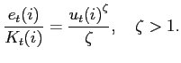
Thus, the firm uses more energy the more intensively it uses its
capital. Capital accumulation is given by
![]() .6
.6
The intermediate goods producing firm also faces a quadratic cost of adjusting its price:
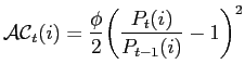
Note that our specification of the adjustment cost function allows for the possibility that firms pay a cost of adjusting price in steady state, so that in steady state the Friedman rule may not be optimal.
Firms choose labor, capital, and utilization to maximize the present discounted value of cash flow:
|
(3.16) |
| (3.17) |
subject to the constraints equation (3.10), equation (3.12, and equation (3.14).
Let
![]() be the
multiplier on constraint equation (3.12) and
be the
multiplier on constraint equation (3.12) and ![]() be the relative price of
energy
be the relative price of
energy
![]() . The
first-order conditions for the firm's optimization problem are then
given by:
. The
first-order conditions for the firm's optimization problem are then
given by:
![\begin{gather*}\begin{array}[c]{rl} \lambda_{t}( 1-\theta) {\left( \frac{P_{t}( i) }{P_{t}}\right) }^{-\theta }\frac{y_{t}}{P_{t}} & +\lambda_{t}\phi( \frac{P_{t}( i) }{P_{t-1}( i) }-1) \frac{1}{P_{t-1}( i) }+\\ \lambda_{t}^{f}{\theta( \frac{P_{t}( i) }{P_{t}}) }^{-\theta-1}\frac{y_{t} }{P_{t}}\mbox{} & +\beta\phi E_{t}\lambda_{t+1}( \frac{P_{t+1}( i) }{P_{t}( i) }-1) \frac{P_{t+1}( i) }{{P_{t}( i) }^{2}}=0 \end{array}\end{gather*}](img48.gif)
Equation (3.18) characterizes the firm's capital rental decision, while equation (3.19) is the optimality condition for its labor input. Equation (3.20) is the optimality condition for utilization, and equation (3.21) describes the firm's optimal pricing decision.
The supply of oil (energy) available to the economy is assumed
exogenous. We interpret this as oil being supplied from a cartel
outside the economy, such as OPEC. In equilibrium, the price of oil
adjusts to equate demand and supply. We examine symmetric
equilibria in which all firms charge the same price and produce the
same quantity of output. Henceforth, we drop the ![]() notation and consider the
representative firm.
notation and consider the
representative firm.
Finally, our benchmark model specification is one for which
historical monetary policy is assumed to have followed a
forward-looking Taylor rule. The central bank sets the nominal
interest rate ![]() as a
function of expected inflation and output:
as a
function of expected inflation and output:
where
![]() is an
inflation target and
is an
inflation target and
![]() is a
measure of potential output. We take potential output to be the
level of output given by a nonmonetary economy (see Woodford (2003)). In the robustness section of the paper, we
also consider a Taylor rule that is a function of contemporaneous
inflation.
is a
measure of potential output. We take potential output to be the
level of output given by a nonmonetary economy (see Woodford (2003)). In the robustness section of the paper, we
also consider a Taylor rule that is a function of contemporaneous
inflation.
In addition to the Taylor rule specifications, the model is also solved and simulated assuming the monetary policymaker is able to commit to an optimal policy. We will then compare the volatility of the economy under optimal policy to the volatility obtained under the historical Taylor rules.
4 Optimal Monetary Policy
Optimal monetary policy is calculated by choosing a money growth rate that maximizes agents' welfare subject to the first-order conditions for the household and the firm and the economy-wide resource constraint. We follow an approach similar to that in Khan et al. (2003) and consider an optimal policy that has been in place for a long enough time that initial conditions do not matter. We use household and firm FOCs' to characterize wages and prices:
 |
||
|
Assume that the cash-in-advance constraint is binding. That, and
the fact that in equilibrium,
![]() allows
gross inflation to be written as
allows
gross inflation to be written as
where
![]() .
Denote
.
Denote
![]() , and
, and
![]() .Combine
the equilibrium conditions to get the following system of
equations:
.Combine
the equilibrium conditions to get the following system of
equations:
| (4.1) | |
| (4.2) | |
|
(4.3) |
|
(4.4) |
![\begin{gather*}\begin{array}[c]{rl} \lambda( 1-\theta) f-\lambda\phi( \frac{g_{-1}c_{1,-1}}{c_{1}}-1) \frac {g_{-1}c_{1,-1}}{c_{1}} & +\lambda^{f}\theta f+\\ \beta E_{t}\lambda^{^{\prime}}( \frac{g c_{1}}{c_{1}^{^{\prime}}}-1) \frac{g c_{1}}{c_{1}^{^{\prime}}} & =0 \end{array}\end{gather*}](img66.gif)
|
(4.5) |
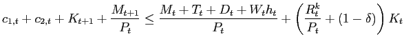
![\begin{gather*}\begin{array}[c]{rl} c_{1}+c_{2}+K^{^{\prime}}-\left( 1-\delta\right) K & +\frac{\lambda^{f} }{\lambda}\frac{f_{u}}{u^{\zeta-1}K}e^{s}+\\ \frac{\phi}{2}{\left( \frac{g_{-1}c_{1,-1}}{c_{1}}-1\right) }^{2} & =f \end{array}\end{gather*}](img67.gif)
|
(4.6) |
Finally, utilization can be expressed as a function of the supply of energy,
4.1 Optimal Policy Lagrangian
Using the lagged multiplier approach as in, for example, Khan et al. (2003), we use equations (23)-(28) to set up a Lagrangian that characterizes the optimal policy problem :
![\begin{displaymath}\begin{array}[c]{rl} \mathcal{L} & =U+\psi_{1}U_{c_{2}}-\psi_{1,-1}\frac{U_{c_{1}}c_{1}} {g_{-1}c_{1,-1}}+ \begin{array}[c]{rl} & \psi_{2}( \lambda^{f}f_{h}+U_{h}) +\psi_{3}U_{c_{2}}+ \end{array} \\ & \psi_{3,-1}\lambda^{f}( f_{k}+\frac{U_{c_{2}}}{\lambda^{f}}\left( 1-\delta\right) -\frac{f_{u}q}{K \zeta}) +\\ & \psi_{4}( U_{c_{2}}( 1-\theta) f-U_{c_{2}}\phi( \frac{g_{-1}c_{1,-1}}{c_{1} }-1) \frac{g_{-1}c_{1,-1}}{c_{1}}+\lambda^{f}\theta f) +\\ & \begin{array}[c]{rl} & \psi_{4,-1}\phi U_{c_{2}}( \frac{g_{-1}c_{1,-1}}{c_{1}}-1) \frac {g_{-1}c_{1,-1}}{c_{1}}+ \end{array} \\ & \begin{array}[c]{rl} & \psi_{5}(c_{1}+c_{2}+K^{^{\prime}}-\left( 1-\delta\right) K+\frac {\lambda^{f}}{U_{c_{2}}}\frac{f_{u}}{q^{\zeta-1}K}e^{s}+\\ & \left. \frac{\phi}{2}{\left( \frac{g_{-1}c_{1,-1}}{c_{1}}-1\right) } ^{2}-f\right) \end{array} \end{array}\end{displaymath}](img70.gif)
|
(4.7) |
The policymaker chooses
![]() to maximize the value of
to maximize the value of
![]() . The
first-order conditions from the maximization problem are linearized
around steady state, and the decision rule for optimal monetary
policy is solved for using a linear system of equations.7 In the simulation exercises, we verify
that the model's outcome does not violate the zero bound on the
nominal interest rate. Because of the assumed form of the
adjustment cost equation, steady state inflation is sufficiently
far from the Friedman rule so that the simulated nominal interest
remains above zero following historical TFP and oil shocks.
. The
first-order conditions from the maximization problem are linearized
around steady state, and the decision rule for optimal monetary
policy is solved for using a linear system of equations.7 In the simulation exercises, we verify
that the model's outcome does not violate the zero bound on the
nominal interest rate. Because of the assumed form of the
adjustment cost equation, steady state inflation is sufficiently
far from the Friedman rule so that the simulated nominal interest
remains above zero following historical TFP and oil shocks.
5 Calibration
We explore several versions of the model: with and without habit
persistence, high and low steady-state markups, forward-looking and
contemporaneous policy rules, and an optimal monetary policy
specification. Utility is specified as in equation (3.1). We chose the parameter
![]() by running a
regression of the consumption velocity of M2 (consumption measured
as nondurables + services) on the 3-month Treasury bill rate. It is
well-known that over the full post-war sample money demand
regressions suffer from parameter instability. We used sample
estimates from a regression estimated over 1964-1979, which
corresponds to the first subsample of our simulation analysis) to
get an implied value of
by running a
regression of the consumption velocity of M2 (consumption measured
as nondurables + services) on the 3-month Treasury bill rate. It is
well-known that over the full post-war sample money demand
regressions suffer from parameter instability. We used sample
estimates from a regression estimated over 1964-1979, which
corresponds to the first subsample of our simulation analysis) to
get an implied value of
![]() . We
then set
. We
then set
![]() .The parameter
.The parameter ![]() on leisure is chosen so that
steady-state hours worked are one-fourth of the time endowment.
on leisure is chosen so that
steady-state hours worked are one-fourth of the time endowment.
On the firm side, we use estimates on markups from Basu and Fernald (1997) to pin down the elasticity of substitution
between goods, ![]() .
Basu and Fernald estimate a markup of about 4 percent for the U.S.
private economy. Our benchmark assumes a steady-state markup of 4
percent -- though our robustness section explores the consequences
of assuming a higher markup of 15 percent. Model parameter values
are reported in Table 2.
.
Basu and Fernald estimate a markup of about 4 percent for the U.S.
private economy. Our benchmark assumes a steady-state markup of 4
percent -- though our robustness section explores the consequences
of assuming a higher markup of 15 percent. Model parameter values
are reported in Table 2.
5.1 TFP Shocks
Variable capital utilization appears to be an empirically important element in calculating an exogenous measure of TFP (see, e.g., paquet and Robidoux (2001)). To compute TFP we follow Burnside and Eichenbaum (1996) and use equation (3.20) to solve for utilization as a function of capital, hours, the real price of oil, and the steady-state markup. We then substitute this expression for utilization into the intermediate goods producing firm's production function. Series on the capital stock, the real price of oil, hours worked, and output are then used to derive an historical measure of TFP. 8
The capital stock series is measured as the net stock of
nonfarm, nonresidential fixed assets and consumer durables. The
aggregate hours series is constructed as average total nonfarm
employment per quarter less employment in the gas and oil
industries times average quarterly hours. The output measure is
real quarterly GDP less farm and housing and ex domestic oil
production. The real oil price series is the price of West Texas
Intermediate divided by the GDP deflator. The oil quantity series
used to calculate GDP ex oil is U.S. crude oil field production.
When solving the model, we assume TFP follows an AR(1) process with
correlation coefficient
![]() .
.
5.2 Price Adjustment
A quadratic price-adjustment specification that has zero cost of adjusting price in steady-state implies a reduced form for inflation
where
![]() ,
mc is the marginal cost of production, and
,
mc is the marginal cost of production, and
![]() is
steady-state inflation. This is the same reduced form as that of
the Calvo (1983) price-setting model, though in the Calvo
specification
is
steady-state inflation. This is the same reduced form as that of
the Calvo (1983) price-setting model, though in the Calvo
specification
![]() with
with
![]() the fixed
probability that a firm must keep its price unchanged in any given
period (see Gali and Gertler (1999)). We calibrated the
price-adjustment cost parameter
the fixed
probability that a firm must keep its price unchanged in any given
period (see Gali and Gertler (1999)). We calibrated the
price-adjustment cost parameter ![]() so that, given
so that, given ![]() and
and
![]() (where
(where
![]() is
chosen to match average GDP deflator inflation), the implied
frequency of price adjustment is four quarters using the mapping
implied by equation (5.1 ).
This led to our setting the price-adjustment cost parameter
is
chosen to match average GDP deflator inflation), the implied
frequency of price adjustment is four quarters using the mapping
implied by equation (5.1 ).
This led to our setting the price-adjustment cost parameter
![]() , which
implies that in steady state, price adjustment costs are about 3
percent of output. To the extent that the price adjustment cost is
high, our model will overpredict the contribution of monetary
policy to the decline in volatility.9
, which
implies that in steady state, price adjustment costs are about 3
percent of output. To the extent that the price adjustment cost is
high, our model will overpredict the contribution of monetary
policy to the decline in volatility.9
Note though that our specification of the adjustment cost function (equation 3.15) implies a positive cost associated with price adjustment in steady state, so that the reduced form for inflation differs somewhat from that in equation (5.1).10 Our results are largely insensitive to these alternative specifications of the price-adjustment cost function. We opted for the cost function (3.15) because it simplifies the comparison of the results with those under optimal monetary policy.11
5.3 Monetary Policy
To characterize historical monetary policy, we assume that systematic policy follows a Taylor rule that sets the short-term nominal interest rate as a function of the output gap and expected inflation (see equation 3.22). We parameterize the policy rule using the estimates in Clarida et al. (2000) for the pre-1979 and the post-1982 periods (see Table 4).12 Clarida et al. estimate a forward-looking rule on GDP deflator inflation and the CBO output gap. Their estimates suggest the Fed increased the nominal funds rate less than one-for-one with expected inflation in the pre-1979 sample which, in their model, leads to indeterminacy. Their post-1982 estimates show that the Fed raised the funds rate more than one-for-one with expected inflation.13
When solving the model using Clarida et al. pre-1979 policy rule estimates, we are able to find a determinate equilibrium even though the Fed responds "passively" to expected inflation. This result is in line with Dupor (2001) who shows that an interest-rate rule for which the monetary authority lowers the real interest rate following a rise in inflation can bring about a unique equilibrium in models with capital accumulation.14
5.4 Oil Sector
Oil supply is treated as exogenous in our simulations, and price is allowed to adjust to changes in supply. To measure exogenous supply, we use the Hamilton (2003) quantitative oil dummy variable that identifies historical episodes in which military conflict led to disruptions in world oil supply. The identified episodes are listed in Table 3.
We treat quantity, rather than price, as exogenous because of the sharp change in the oil market over the postwar period. While Hamilton (1983, 1985) convincingly argues that the price of oil can be taken as exogenous during the period 1948-1972, since the end of the 1970s, the time series properties of the price of oil are much different, and the price appears to be much more affected in the short run by world demand conditions. These facts pose a challenge for a model that assumes exogenous oil prices when accounting for the change in economic volatility over the postwar era. Our solution of treating quantity as exogenous is not without problems though-the method allows domestic TFP to affect the price of oil prior to 1973. We are assuming that treating quantity, rather than price, as exogenous leads to more consistent treatment of the oil market pre-1973 and post-1973.
In the model simulations it is assumed that the quantity of oil
used in the economy is constant except for the disruptions
identified by Hamilton (2003). The quantity
disruptions are assumed to last for one quarter, after which time
the oil quantity series returns to its baseline level. When solving
the model, the oil quantity disruption series is assumed to be
i.i.d.15 We set
the steady state supply of oil so that, conditional on the other
parameter values, the model matches as closely as possible the
decline in real output and inflation volatility between our two
subsamples.16 Finally,
the parameter ![]() , which
governs the elasticity of the energy-capital ratio with respect to
utilization, is set so that the average share of oil in the model
economy matches that in the U.S. data, which is about 3.3
percent.
, which
governs the elasticity of the energy-capital ratio with respect to
utilization, is set so that the average share of oil in the model
economy matches that in the U.S. data, which is about 3.3
percent.
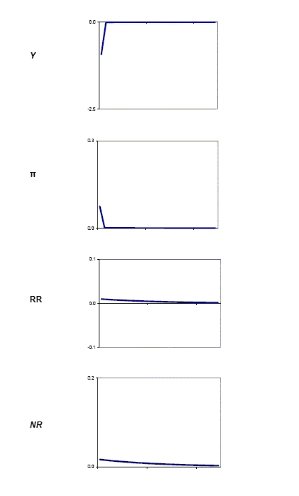
Figure 3 shows the response of output, inflation, and interest rates to a 10 percent decrease in the supply of oil.17 The negative oil shock leads to a transitory drop in real output that lasts about one quarter (recall that the oil quantity shock is i.i.d and so has no persistence). The real interest rises as credit good consumption drops on impact and then increases monotonically back to the steady state. The drop in output puts upward pressure on prices and inflation, which the monetary authority partially offsets by raising the nominal interest rate. Overall, a negative oil shock in our model has similar effects to a temporary drop in TFP.
6 Benchmark Model Results
Our benchmark model is one for which there are no habits in preferences, monetary policy follows a forward-looking rule as in equation (3.22), and the steady-state markup is 4 percent. The model is simulated over two subsamples: 1964Q1 to 1979Q2 and 1984Q2 to 1999Q3. We chose to end the sample in 1999Q3 so that the subsamples are of equal length. The 1979Q3 to 1984Q4 period is dropped from the analysis for two reasons. First, many studies date a break in monetary policy at the beginning of the Volcker regime in October 1979. At the same time, statistical evidence puts the break in real output volatility around 1984Q1, and as seen in Table 1, whether or not the 1980-1983 data are included in the volatility calculations has a significant effect on the resulting statistics. Second, Sims and Zha (2002) argue that the episode from 1980 to 1982 appears to be different in terms of monetary policy, and that it is not the case that there was a dramatic shift in policy between the 1960-78 period and the 1983-2000 period.
The models for which monetary policy is assumed to follow a Taylor rule are linearized and solved using the method described in King and Watson (1998). Solutions are found for the pre-1979 and post-1984 calibrations. The models are then simulated assuming the pre-1979 and post-1984 economies are independent.18 Thus, we implicitly assume that households in the pre-1979 subsample thought the monetary policy rule would forever stay at its pre-1979 calibration. Transition dynamics between the regimes are not modeled. The form of the monetary policy rule requires a measure of potential output. When calculating the level of potential output, we use the state variables that evolve under the assumption that the economy is always in a nonmonetary, flexible-price equilibrium.
6.1 Contributions to the Decline in Volatility
Consider now the model's implications for output and inflation volatility in the pre-1979 and post-1984 periods. Panel A of Table 5 shows that the benchmark model predicts a decline in real output volatility of nearly the same magnitude as the data. Empirically, the standard deviation of real output falls 45 percent, from 2.11 percent to 1.16 percent. The benchmark model implies a fall in real output volatility of 41 percent, from 2.27 percent to 1.35 percent. The model slightly overpredicts the volatility of output in the two subperiods.
Panel B of Table 5 shows that the benchmark specification is close to matching the decline in the standard deviation of inflation from the pre-1979 to the post-1984 period, predicting a decline in inflation volatility of about 51 percent, compared to 54 percent in the data. The model underpredicts the levels of inflation volatility in both sub-periods: the benchmark specification accounts for only 20 percent of the standard deviation of inflation.
Table 6 shows the contribution of monetary policy, oil shocks, and TFP shocks to the decline in real output volatility. These contributions are measured as follows:
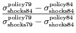
|
||
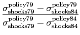
|
where
![]() represents, for example, the standard deviation of hp-filtered
output from a model simulation that has a policy rule parameterized
for the pre-1979 specification and where the post-1984 exogenous
oil and TFP shock series are fed in. Thus, the monetary policy
contribution measures the fraction of the decline in output
volatility that would occur if the pre-1979 monetary policy rule
had been in place in the post-1984 shock environment. Our
contribution measures isolate the effect of changing a single
policy or shock sequence, holding everything else constant. We did
not separately calculate the contribution of oil shocks and TFP
shocks using this decomposition because there are only 3 oil shocks
(by our measure) that occurred over the sample - two in the
pre-1979 period and one in post-1984 period. For the counterfactual
exercises, we found the results were sensitive to where the oil
shocks were placed in time: ie. whether they fell in an expansion
or a recession period.
represents, for example, the standard deviation of hp-filtered
output from a model simulation that has a policy rule parameterized
for the pre-1979 specification and where the post-1984 exogenous
oil and TFP shock series are fed in. Thus, the monetary policy
contribution measures the fraction of the decline in output
volatility that would occur if the pre-1979 monetary policy rule
had been in place in the post-1984 shock environment. Our
contribution measures isolate the effect of changing a single
policy or shock sequence, holding everything else constant. We did
not separately calculate the contribution of oil shocks and TFP
shocks using this decomposition because there are only 3 oil shocks
(by our measure) that occurred over the sample - two in the
pre-1979 period and one in post-1984 period. For the counterfactual
exercises, we found the results were sensitive to where the oil
shocks were placed in time: ie. whether they fell in an expansion
or a recession period.
Table 6 shows that under the benchmark calibration the change in systematic monetary policy accounted for about 17 percent of the decline in real output volatility, implying that the change in the behavior of TFP shocks and oil shocks accounted for 83 percent of the real output volatility drop. For inflation volatility, the change in systematic policy has a bigger effect, accounting for about 29 percent of the drop in the standard deviation of inflation.
Although we did not calculate the direct contribution of oil shocks to the decline in volatility, Table 7 provides evidence on the importance of oil shocks for business cycle volatility in the two sub-periods. To measure that contribution, we compare the volatility predictions of a model that has both TFP and oil shocks to one that has TFP shocks only. In the pre-1979 specification, oil shocks account for about 3 percent of the standard deviation of output and about 4 percent of the standard deviation of inflation. In the post-1984 period, the contribution is larger: 9 percent of the standard deviation of output and 19 percent of the standard deviation of inflation. Thus, our simulations suggest that oil shocks play a substantially larger role in accounting for the business-cycle volatility of output and inflation volatility in the post-1984 period. This occurs not because of an increase in oil shocks in the post-1984 period (in fact, there are fewer), but rather because of the general reduction in volatility due to other shocks.
6.2 Optimal Monetary Policy
Consider now the behavior of the model economy under our calculated optimal policy with commitment. Table 8 shows the volatilities of output and inflation as implied by the model's structure when monetary policy is set optimally. Panel B indicates that under the Ramsey plan, the planner attempts to keep inflation constant. This complements Khan et al. (2003), who find a similar result in a framework without capital. As noted in Khan et al. (2003), there is a tension between eliminating the distortion that arises from price rigidity and eliminating the distortion that arises from a positive nominal interest rate. In our framework, as in theirs, the planner sets the variance of inflation to almost zero, so that the economy's sticky-price distortion is eliminated. Consequently, the Friedman rule is not optimal.
The model predicts that real output volatility would have been lower than what was observed in the historical data had policy been set according to the Ramsey plan. When the planner keeps inflation roughly constant, the decline in real output volatility between the pre-1979 and the post-1984 eras is 41 percent versus the 45-percent decline measured from the U.S. data. Real output volatility in the pre-1979 period drops by about 25 percent under optimal policy compared to the data. By reducing the volatility of inflation, the planner reduces the effects of the inflation tax, which lowers the fluctuations in labor and capital inputs, and ultimately in output.
Figures 4 plots the response of the economy to a negative 1 percent TFP shock under optimal monetary policy, as well as under the benchmark calibration.19 The drop in TFP lowers output below the steady state and puts upward pressure on the rate of inflation. To offset the expected upward pressure on prices, the monetary authority lowers the growth rate of money, which in equilibrium lowers the rate of inflation on impact. Since the post-1984 interest-rate rule places relatively more weight on expected inflation compared to the pre-1979 policy rule, the movement in the inflation rate is more stable in the post-1984 period than in the pre-1979 one. Along the inflation dimension, the post-1984 monetary authority's response to a TFP shock is relatively closer to the optimal response, which keeps the inflation rate constant.
The output and real interest rate responses to the TFP shock are similar across the two non-optimal policy regimes, which bears out the finding that the change in systematic policy plays a relatively small role in accounting for the real output volatility decline. Under optimal monetary policy, the decline in TFP still leads to a drop in output and the real interest rate, but the output response is both muted and smoother than under the benchmark specification.
An important difference between the model under optimal policy and under the pre-1979 or post-1984 Taylor rules is the behavior of markups. King and Goodfriend (1997) argue that markups act like distortionary taxes and that optimal policy should therefore attempt to keep them constant. Indeed, we find that under optimal monetary policy, markup variability is largely eliminated. Output volatility is reduced under optimal monetary policy in part because reducing the volatility of the markup lowers the variation in labor and capital inputs, which ultimately results in more stable real output Model simulations suggest that markup volatility is about 5 percent lower under the post-84 monetary policy rule when compared to the pre-79 policy rule. Hence, the post-84 rule appears to be closer to optimal.
6.3 Sensitivity Analysis
The robustness of the results is checked by analyzing different model specifications. We chose first to vary the type of interest-rate rule that characterizes monetary policy, switching from a forward-looking rule to a contemporaneous rule:
The parameters of the alternative rule are the same as under the benchmark (see Table 4).
Since habit formation has been shown to help explain the impact of monetary shocks on variables, as well as explain several asset-pricing puzzles, we also examine the sensitivity of the results to a specification that introduces internal habits. Accordingly, the utility function is:
In addition, we also examine a specification that calibrates the steady-state markup at 15 percent, which could potentially lead to a higher contribution of monetary policy.
The performance of the alternative specifications and the implied contributions of monetary policy and exogenous shocks under the alternatives are reported in Tables 5 and 6. Table 5, Panel A, shows that the contemporaneous Taylor rule results in an output volatility drop that underpredicts that in the data, while the model with habit persistence generates a slightly larger decline in real output volatility relative to the benchmark and the data. The high markup model shows the smallest drop in real output volatility, since it makes the post-1984 period too volatile.
The implications of the alternative specifications for inflation volatility are reported in Table 5, panel B. All of the specifications continue to underpredict the level of inflation volatility. The high markup specification comes closest to matching inflation volatility in the pre-1979 period, though it overpredicts the decline. The contemporaneous policy rule and habit persistence specifications predict a decline in inflation volatility that is similar to that of the benchmark model.
Overall, Table 6 indicates that the alternative model specifications lead to reasonably similar contributions of monetary policy to the decline in real output and inflation volatility. Though the model with habit persistence predicts that monetary policy's contribution to the decline in output volatility was somewhat higher than the other specifications, reaching 26 percent. For the case of the drop in inflation volatility, the high-markup specification suggests a much larger role for policy as 61 percent of the decline in inflation volatility can be attributed to change in systematic monetary policy.
Finally, Table 8 shows that the introduction of habit formation does not change the benchmark optimal monetary policy results in any significant way.
We conclude that alternative specifications of our model are largely in line with our benchmark findings. Although the change in monetary policy played a role in the postwar moderation of output volatility, most of the decline can be attributed to a reduction in the volatility of TFP and oil shocks. The robustness analysis suggests that the change in monetary policy accounted for 15-25 percent of the fall in output volatility, which is in line with the VAR evidence in Stock and Watson (2002). In contrast, we do find that monetary policy played a relatively more important role in stabilizing inflation, in most cases around 30 percent, but up to 60 percent under higher markups.
7 Conclusion
We used a structural model to assess the relative contributions of monetary policy, TFP shocks, and oil shocks to the decline in volatility of U.S. real output and inflation. In line with the empirical results in Stock and Watson (2002), our benchmark model predicts that monetary policy played a relatively small role in the decline in volatility of real output, accounting for about 17 percent of the drop. On the other hand, it suggests that monetary policy accounted for about 30 percent of the decline in inflation volatility. The model suggests that smaller TFP shocks and oil shocks are the principal cause of the more stable real economy post-1984. An important component of the analysis is the calculation of optimal monetary policy in a model with endogenous capital accumulation. Relative to the estimated historical Taylor rules, optimal policy would have virtually eliminated inflation variability and significantly lowered real output volatility.
References
Ahmed, S., Levin, A., Wilson, B. A., 2004. Recent U.S. macroeconomic stability: Good policies, good practices or good luck. Review of Economics and Statistics 86, 824�832.
Arias, A., Hansen, G., Ohanian, L., 2006. Why have business cycle fluctuations become less volatile? NBER Working Paper 12-79.
Basu, S., Fernald, J. G., 1997. Returns to scale in U.S. production: Estimates and implications. Journal of Political Economy 105, 249�283.
Basu, S., Fernald, J. G., Kimball, M., 2004. Are technology improvements contractionary? National Burea of Economic ResearchWorking Paper No. 10592.
Bils, M., Klenow, P. J., 2002. Some evidence on the importance of sticky prices. National Bureau of Economic Research Working Paper No. 9069.
Blanchard, O., Simon, J., 2001. The long and large decline in U.S. ouput volatility. Brookings Papers on Economic Acitivity 2001:1, 135�164.
Boivin, J., Giannoni, M., 2003. Has monetary policy become more effective? National Bureau of Economic Research Working Paper No. 9459.
Bullard, J., Eusepi, S., 2003. Did the great inflation occur despite policymaker commitment to a taylor rule? Fderal Reserve Bank of St. Louis Working Paper 2003-013.
Burnside, C., Eichenbaum, M., 1996. Factor-hoarding and the propagation of business cycle shocks. American Economic Review 86, 1154�1174.
Christiano, L. J., Eichenbaum, M., Evans, C. L., 2005. Nominal rigidities and the dynamic effects of a shock to monetary policy. Journal of Political Economy 113, 1�45.
Clarida, R., Gali, J., Gertler, M., 2000. Monetary policy rules and macroeconomic stability: Evidence and some theory. Quarterly Journal of Economics 115, 147�180.
Dupor, W., 2001. Investment and interest rate policy. Journal of Economic Theory 98, 85�113.
Erceg, C., Henderson, D. W., Levin, A., 2000. Optimal monetary policy with staggered wage and price contracts. Journal of Monetary Economics 46, 281�313.
Finn, M. G., 1995. Variance properties of solow�s productivity residual and their cyclical implications. Journal of Economic Dynamics and Control 19, 1249�1282.
Gal�, J., Gertler, M., 1999. Inflation dynamics: A structural econometric analysis. Journal of Monetary Economics 44, 195�222.
Gal�, J., L�pez-Salido, Vall�s, J., 2003. Technology shocks and monetary policy: Assessing the fed�s performance. Journal of Monetary Economics 50, 723�743.
Hamilton, J. D., 1983. Oil and the macroeconomy since world war II. Journal of Political Economy 91, 228�248.
Hamilton, J. D., 1985. Historical causes of postwar oil shocks and recessions. Energy Journal 6, 97�116.
Hamilton, J. D., 2003. What is an oil shock? Journal of Econometrics 113, 363�398.Ireland, P., 2001. Sticky-price models of the business cycle: Specification and stability. Journal of Monetary Economics 47, 3�18.
Khan, A., King, R. G., Wolman, A. L., 2003. Optimal monetary policy. Review of Economic Studies 70, 825�860.
Kim, C., Nelson, C., 1999. Has the U.S. economy become more stable? a bayesian approach based on a markov-switching model of the business cycle. The Review of Economics and Statistics 81, 608�616.
King, R. G., Goodfriend, M., 1997. The new neoclassical synthesis and the role of monetary policy. In: NBER Macroeconomics Annual. MIT Press, Cambridge and London, pp. 231�83.
King, R. G., Watson, M. W., 1998. The solution of singular linear difference systems under rational expectations. International Economic Review 39, 1015�1026.
Kollman, R., 2003. Welfare maximizing fiscal and monetary policy rules. Center for Economic Policy Research.
Lubik, T. A., Schorfheide, F., 2004. Testing for indeterminacy: An application to U.S. monetary policy. American Economic Review 94, 190�217.
Lucas, R. E., Stokey, N. L., 1987. Money and interest in a cash-in-advance economy. Econometrica 55 (3), 491�513.
McConnell, M. M., Perez-Quiros, G., 2000. Output fluctuations in the united states: What has changed since the early 1980s. American Economic Review 90, 1464�1476.
Orphanides, A., 2004. Monetary policy rules, macroeconomic stability and inflation: A veiw from the trenches. Journal ofMoney, Credit, and Banking 36, 151�176.
Paquet, A., Robidoux, B., 2001. Issues on the measurement of the solow residual and the testing of its exogeneity: Evidence for canada. Journal of Monetary Economics 47, 595�612.
Primiceri, G. E., 2003. Time varying structural vector autoregressions and monetary policy. Princeton University Working Paper.
Sbordone, A., 2002. Prices and unit labor costs: A new test of price stickiness. Journal of Monetary Economics 49, 265�292.
Schmitt-Groh�, S., Uribe, M., 2004. Optimal simple and implementable monetary and fiscal policy rules. Manuscript, Duke University.
Sims, C. J., Zha, T., 2002. Macroeconomic switching.
Stock, J. H., Watson, M. W., 2002. Has the business cycle changed and why? In: NBER Macroeconomics Annual. National Bureau of Economic Research.
Stock, J. H., Watson, M.W., 2003. Has the business cycle changed? evidence and explanations. In: Monetary Policy and Uncertainty. Federal Reserve Bank of Kansas City.
Taylor, J. B., 2000. Remarks for panel discussion on recent changed in trend and cycle. SIEPR Conference.
Woodford, M., 2003. Interest and Prices: Foundations of a Theory of Monetary Policy. Princeton University Press, Princeton and Oxford.
Table 1: Ouput and Inflation Standard Deviations
| 60s | 70s | 80s | 90s | pre-1979 | Post-1979 | Pre-1984 | post-1984 | |
|---|---|---|---|---|---|---|---|---|
| GDP | 0.879 | 1.094 | 0.969 | 0.531 | 1.008 | 0.777 | 1.081 | 0.485 |
| Inf | 0.381 | 0.529 | 0.604 | 0.239 | 0.664 | 0.538 | 0.699 | 0.250 |
Table 2: Benchmark model calibration
| Parameter | Value |
|---|---|
| 0.99 | |
| 0.65 | |
|
|
0.025 |
| 24.5 | |
| 8.97 | |
| 266.6 | |
| 2.68 | |
| 0.28 | |
| 0.95 | |
|
|
0 |
Table 3: Hamilton (2001) Quantitative oil dummy: Exogenous changes in world oil supply
| Date | Event | Drop in world production |
|---|---|---|
| Nov. 1973 | Arab-Israeli War | 7.8% |
| Dec. 1978 | Iranian Revolution | 8.9% |
| Oct. 1980 | Iran-Iraq War | 7.2% |
| Aug. 1990 | Persian Gulf War | 8.8% |
Table 4: Monetary policy rule parameterization:
| Rule | |||
|---|---|---|---|
| CGG: 69Q2-79Q2 | 0.68 | 0.83 | 0.27 |
| CGG: 83Q1-96Q4 | 0.91 | 1.58 | 0.15 |
Table 5: Output and Inflation Volatility (in %): Panel A: Standard Deviation of Output
| Pre-1979 | Post-1984 | Decline | |
|---|---|---|---|
| Data | 2.11 | 1.16 | -45.0 |
| Models: Benchmark Model | 2.27 | 1.35 | -40.9 |
| Models: Contemporaneous Rule | 2.11 | 1.31 | -38.0 |
| Models: Habit Persistence | 2.11 | 1.12 | -46.6 |
| Models: Higher Markup | 2.11 | 1.61 | -23.6 |
Table 5: Output and Inflation Volatility (in %): Panel B: Standard Deviation of Inflation
| Pre-1979 | Post-1984 | Decline | |
|---|---|---|---|
| Data | 0.37 | 0.17 | -54.1 |
| Models: Benchmark Model | 0.056 | 0.027 | -51.4 |
| Models: Contemporaneous Rule | 0.043 | 0.022 | -48.0 |
| Models: Habit Persistence | 0.050 | 0.025 | -50.5 |
| Models: Higher Markup | 0.189 | 0.045 | -76.2 |
Table 6: Contribution of Monetary Policy to the Decline in Inflation and Output Volatility (in %) (Markup=1.04): Panel A: Output
| Policy | Shocks | |
|---|---|---|
| Models: Benchmark Model | 16.7 | 83.3 |
| Models: Contemporaneous Rule | 14.5 | 85.5 |
| Models: Habit Persistence | 26.3 | 73.7 |
| Models: Higher Markup | 17.6 | 82.4 |
Table 6: Contribution of Monetary Policy to the Decline in Inflation and Output Volatility (in %) (Markup=1.04): Panel B: Inflation
| Policy | Shocks | |
|---|---|---|
| Models: Benchmark Model | 28.6 | 71.4 |
| Models: Contemporaneous Rule | 32.2 | 67.8 |
| Models: Habit Persistence | 32.4 | 67.6 |
| Models: Higher Markup | 61.0 | 39.0 |
Table 7: Business Cycle Contributions of Oil Shocks (in %): Panel A: Standard Deviation of Output
| Pre-1979 | Post-1984 | |
|---|---|---|
| Data | 2.11 | 1.16 |
| Benchmark Model: With tfp and oil shocks | 2.27 | 1.35 |
| Benchmark Model: With tfp shocks only | 2.20 | 1.23 |
| Benchmark Model: Oil shocks contribution | 3.1 | 8.9 |
Table 7: Business Cycle Contributions of Oil Shocks (in %): Panel B: Standard Deviation of Inflation
| Pre-1979 | Post-1984 | |
|---|---|---|
| Data | 0.37 | 0.17 |
| Models: With tfp and oil shocks | 0.056 | 0.027 |
| Models: With tfp shocks only | 0.054 | 0.022 |
| Models: Oil shocks contribution | 3.6 | 18.5 |
Table 8: Output and Inflation Volatility Under Optimal Policy (%): Panel A: Standard Deviation of Output
| Pre-1979 | Post-1984 | |
|---|---|---|
| Data | 2.11 | 1.16 |
| Models: Benchmark Model* | 1.56 | 0.92 |
| Models: Habit Persistence | 1.53 | 0.90 |
Table 8: Output and Inflation Volatility Under Optimal Policy (%): Panel B: Standard Deviation of Inflation
| Pre-1979 | Post-1984 | |
|---|---|---|
| Data | 0.37 | 0.17 |
| Models: Benchmark Model | 0.002 | 0.001 |
| Models: Habit Persistence | 0.002 | 0.001 |
Figure 1: 100*Standard deviation hp-filtered real GDP, 8-quarter rolling window: STD HP-filtered Real GDP
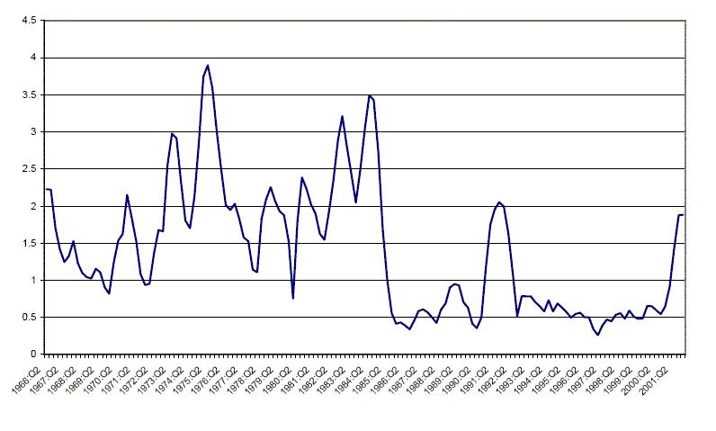
Data for Figure 1: 100*Standard deviation hp-filtered real GDP, 8-quarter rolling window: STD HP-filtered Real GDP
| Standard Deviation of HP-filtered output std(hp(dlog(y))) | |
|---|---|
| 1966:Q1 | 2.019356 |
| 1966:Q2 | 2.228109 |
| 1966:Q3 | 2.220095 |
| 1966:Q4 | 1.697423 |
| 1967:Q1 | 1.416247 |
| 1967:Q2 | 1.24432 |
| 1967:Q3 | 1.3268 |
| 1967:Q4 | 1.527953 |
| 1968:Q1 | 1.230542 |
| 1968:Q2 | 1.098015 |
| 1968:Q3 | 1.041814 |
| 1968:Q4 | 1.023726 |
| 1969:Q1 | 1.154909 |
| 1969:Q2 | 1.105366 |
| 1969:Q3 | 0.90557 |
| 1969:Q4 | 0.817925 |
| 1970:Q1 | 1.235326 |
| 1970:Q2 | 1.533404 |
| 1970:Q3 | 1.623072 |
| 1970:Q4 | 2.151572 |
| 1971:Q1 | 1.843589 |
| 1971:Q2 | 1.533889 |
| 1971:Q3 | 1.084549 |
| 1971:Q4 | 0.93705 |
| 1972:Q1 | 0.952586 |
| 1972:Q2 | 1.369583 |
| 1972:Q3 | 1.678329 |
| 1972:Q4 | 1.658382 |
| 1973:Q1 | 2.551838 |
| 1973:Q2 | 2.976776 |
| 1973:Q3 | 2.913498 |
| 1973:Q4 | 2.330519 |
| 1974:Q1 | 1.80678 |
| 1974:Q2 | 1.70154 |
| 1974:Q3 | 2.121794 |
| 1974:Q4 | 2.862511 |
| 1975:Q1 | 3.744181 |
| 1975:Q2 | 3.898208 |
| 1975:Q3 | 3.589721 |
| 1975:Q4 | 2.996915 |
| 1976:Q1 | 2.477062 |
| 1976:Q2 | 2.015575 |
| 1976:Q3 | 1.946754 |
| 1976:Q4 | 2.031543 |
| 1977:Q1 | 1.830917 |
| 1977:Q2 | 1.577796 |
| 1977:Q3 | 1.525802 |
| 1977:Q4 | 1.14229 |
| 1978:Q1 | 1.109293 |
| 1978:Q2 | 1.830528 |
| 1978:Q3 | 2.088186 |
| 1978:Q4 | 2.254284 |
| 1979:Q1 | 2.06977 |
| 1979:Q2 | 1.929847 |
| 1979:Q3 | 1.877981 |
| 1979:Q4 | 1.532945 |
| 1980:Q1 | 0.753995 |
| 1980:Q2 | 1.800068 |
| 1980:Q3 | 2.386272 |
| 1980:Q4 | 2.230514 |
| 1981:Q1 | 2.020393 |
| 1981:Q2 | 1.899369 |
| 1981:Q3 | 1.625927 |
| 1981:Q4 | 1.545666 |
| 1982:Q1 | 1.918377 |
| 1982:Q2 | 2.345273 |
| 1982:Q3 | 2.880073 |
| 1982:Q4 | 3.213276 |
| 1983:Q1 | 2.801122 |
| 1983:Q2 | 2.433621 |
| 1983:Q3 | 2.046852 |
| 1983:Q4 | 2.484279 |
| 1984:Q1 | 3.045148 |
| 1984:Q2 | 3.495435 |
| 1984:Q3 | 3.427721 |
| 1984:Q4 | 2.73983 |
| 1985:Q1 | 1.695372 |
| 1985:Q2 | 1.000402 |
| 1985:Q3 | 0.55466 |
| 1985:Q4 | 0.413999 |
| 1986:Q1 | 0.432341 |
| 1986:Q2 | 0.390262 |
| 1986:Q3 | 0.338558 |
| 1986:Q4 | 0.452646 |
| 1987:Q1 | 0.585736 |
| 1987:Q2 | 0.607033 |
| 1987:Q3 | 0.567993 |
| 1987:Q4 | 0.500575 |
| 1988:Q1 | 0.424982 |
| 1988:Q2 | 0.602268 |
| 1988:Q3 | 0.686509 |
| 1988:Q4 | 0.903689 |
| 1989:Q1 | 0.947774 |
| 1989:Q2 | 0.93242 |
| 1989:Q3 | 0.703822 |
| 1989:Q4 | 0.632512 |
| 1990:Q1 | 0.4122 |
| 1990:Q2 | 0.354831 |
| 1990:Q3 | 0.498467 |
| 1990:Q4 | 1.162992 |
| 1991:Q1 | 1.750729 |
| 1991:Q2 | 1.95778 |
| 1991:Q3 | 2.051357 |
| 1991:Q4 | 1.995014 |
| 1992:Q1 | 1.639245 |
| 1992:Q2 | 1.096024 |
| 1992:Q3 | 0.51645 |
| 1992:Q4 | 0.786327 |
| 1993:Q1 | 0.784758 |
| 1993:Q2 | 0.784101 |
| 1993:Q3 | 0.708436 |
| 1993:Q4 | 0.650467 |
| 1994:Q1 | 0.581867 |
| 1994:Q2 | 0.730246 |
| 1994:Q3 | 0.579338 |
| 1994:Q4 | 0.686052 |
| 1995:Q1 | 0.631499 |
| 1995:Q2 | 0.569923 |
| 1995:Q3 | 0.495856 |
| 1995:Q4 | 0.544543 |
| 1996:Q1 | 0.562863 |
| 1996:Q2 | 0.502053 |
| 1996:Q3 | 0.500452 |
| 1996:Q4 | 0.338807 |
| 1997:Q1 | 0.261916 |
| 1997:Q2 | 0.390727 |
| 1997:Q3 | 0.471238 |
| 1997:Q4 | 0.446246 |
| 1998:Q1 | 0.534852 |
| 1998:Q2 | 0.555996 |
| 1998:Q3 | 0.482093 |
| 1998:Q4 | 0.590551 |
| 1999:Q1 | 0.510525 |
| 1999:Q2 | 0.480028 |
| 1999:Q3 | 0.487158 |
| 1999:Q4 | 0.652782 |
| 2000:Q1 | 0.650952 |
| 2000:Q2 | 0.596061 |
| 2000:Q3 | 0.545014 |
| 2000:Q4 | 0.646344 |
| 2001:Q1 | 0.912236 |
| 2001:Q2 | 1.421965 |
| 2001:Q3 | 1.877354 |
| 2001:Q4 | 1.883231 |
Figure 2: Standard Deviation of HP-filtered delta ln(P sub t), 8-quarter rolling window
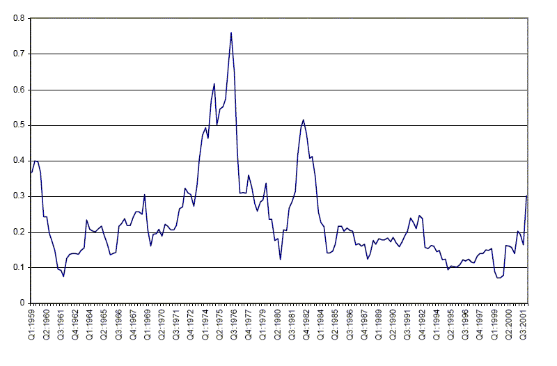
Data for Figure 2: Standard Deviation of HP-filtered delta ln(P sub t), 8-quarter rolling window: STD GDP Deflator Inflation
| Standard Deviation of GDP Inflation | |
|---|---|
| Q1:1959 | 0.366903 |
| Q2:1959 | 0.400108 |
| Q3:1959 | 0.397285 |
| Q4:1959 | 0.367033 |
| Q1:1960 | 0.242286 |
| Q2:1960 | 0.242368 |
| Q3:1960 | 0.198156 |
| Q4:1960 | 0.171372 |
| Q1:1961 | 0.147727 |
| Q2:1961 | 0.096319 |
| Q3:1961 | 0.091823 |
| Q4:1961 | 0.075611 |
| Q1:1962 | 0.126493 |
| Q2:1962 | 0.137781 |
| Q3:1962 | 0.139676 |
| Q4:1962 | 0.139551 |
| Q1:1963 | 0.137659 |
| Q2:1963 | 0.149312 |
| Q3:1963 | 0.155526 |
| Q4:1963 | 0.234629 |
| Q1:1964 | 0.207367 |
| Q2:1964 | 0.202373 |
| Q3:1964 | 0.200331 |
| Q4:1964 | 0.209789 |
| Q1:1965 | 0.216582 |
| Q2:1965 | 0.192603 |
| Q3:1965 | 0.167018 |
| Q4:1965 | 0.137079 |
| Q1:1966 | 0.139969 |
| Q2:1966 | 0.144086 |
| Q3:1966 | 0.216988 |
| Q4:1966 | 0.22342 |
| Q1:1967 | 0.237387 |
| Q2:1967 | 0.217972 |
| Q3:1967 | 0.218485 |
| Q4:1967 | 0.243609 |
| Q1:1968 | 0.256723 |
| Q2:1968 | 0.257122 |
| Q3:1968 | 0.250052 |
| Q4:1968 | 0.305612 |
| Q1:1969 | 0.208666 |
| Q2:1969 | 0.160179 |
| Q3:1969 | 0.19349 |
| Q4:1969 | 0.195346 |
| Q1:1970 | 0.207309 |
| Q2:1970 | 0.188906 |
| Q3:1970 | 0.221789 |
| Q4:1970 | 0.21581 |
| Q1:1971 | 0.205268 |
| Q2:1971 | 0.205289 |
| Q3:1971 | 0.218182 |
| Q4:1971 | 0.266018 |
| Q1:1972 | 0.270046 |
| Q2:1972 | 0.323084 |
| Q3:1972 | 0.308728 |
| Q4:1972 | 0.305325 |
| Q1:1973 | 0.272305 |
| Q2:1973 | 0.328863 |
| Q3:1973 | 0.405704 |
| Q4:1973 | 0.471437 |
| Q1:1974 | 0.491937 |
| Q2:1974 | 0.462226 |
| Q3:1974 | 0.56883 |
| Q4:1974 | 0.615743 |
| Q1:1975 | 0.500311 |
| Q2:1975 | 0.545625 |
| Q3:1975 | 0.552697 |
| Q4:1975 | 0.572078 |
| Q1:1976 | 0.676925 |
| Q2:1976 | 0.75995 |
| Q3:1976 | 0.649201 |
| Q4:1976 | 0.420561 |
| Q1:1977 | 0.308389 |
| Q2:1977 | 0.310796 |
| Q3:1977 | 0.308685 |
| Q4:1977 | 0.360065 |
| Q1:1978 | 0.326436 |
| Q2:1978 | 0.278615 |
| Q3:1978 | 0.258911 |
| Q4:1978 | 0.284006 |
| Q1:1979 | 0.289831 |
| Q2:1979 | 0.337683 |
| Q3:1979 | 0.235254 |
| Q4:1979 | 0.235729 |
| Q1:1980 | 0.176326 |
| Q2:1980 | 0.180984 |
| Q3:1980 | 0.123067 |
| Q4:1980 | 0.205853 |
| Q1:1981 | 0.204433 |
| Q2:1981 | 0.266416 |
| Q3:1981 | 0.286816 |
| Q4:1981 | 0.314904 |
| Q1:1982 | 0.417991 |
| Q2:1982 | 0.492656 |
| Q3:1982 | 0.514754 |
| Q4:1982 | 0.47457 |
| Q1:1983 | 0.407203 |
| Q2:1983 | 0.412463 |
| Q3:1983 | 0.354899 |
| Q4:1983 | 0.256179 |
| Q1:1984 | 0.227942 |
| Q2:1984 | 0.215242 |
| Q3:1984 | 0.141211 |
| Q4:1984 | 0.142108 |
| Q1:1985 | 0.146893 |
| Q2:1985 | 0.165204 |
| Q3:1985 | 0.216186 |
| Q4:1985 | 0.216923 |
| Q1:1986 | 0.20314 |
| Q2:1986 | 0.210725 |
| Q3:1986 | 0.20419 |
| Q4:1986 | 0.202647 |
| Q1:1987 | 0.163871 |
| Q2:1987 | 0.168338 |
| Q3:1987 | 0.160089 |
| Q4:1987 | 0.165723 |
| Q1:1988 | 0.123326 |
| Q2:1988 | 0.137518 |
| Q3:1988 | 0.176375 |
| Q4:1988 | 0.165244 |
| Q1:1989 | 0.182152 |
| Q2:1989 | 0.178309 |
| Q3:1989 | 0.178672 |
| Q4:1989 | 0.18409 |
| Q1:1990 | 0.17278 |
| Q2:1990 | 0.185567 |
| Q3:1990 | 0.169841 |
| Q4:1990 | 0.159271 |
| Q1:1991 | 0.171627 |
| Q2:1991 | 0.191011 |
| Q3:1991 | 0.203266 |
| Q4:1991 | 0.239232 |
| Q1:1992 | 0.225298 |
| Q2:1992 | 0.210137 |
| Q3:1992 | 0.246752 |
| Q4:1992 | 0.238351 |
| Q1:1993 | 0.156539 |
| Q2:1993 | 0.154563 |
| Q3:1993 | 0.16177 |
| Q4:1993 | 0.160753 |
| Q1:1994 | 0.144795 |
| Q2:1994 | 0.149159 |
| Q3:1994 | 0.122308 |
| Q4:1994 | 0.124128 |
| Q1:1995 | 0.094576 |
| Q2:1995 | 0.103978 |
| Q3:1995 | 0.103765 |
| Q4:1995 | 0.102027 |
| Q1:1996 | 0.108011 |
| Q2:1996 | 0.122782 |
| Q3:1996 | 0.118953 |
| Q4:1996 | 0.123356 |
| Q1:1997 | 0.115744 |
| Q2:1997 | 0.112688 |
| Q3:1997 | 0.133279 |
| Q4:1997 | 0.139112 |
| Q1:1998 | 0.138922 |
| Q2:1998 | 0.150985 |
| Q3:1998 | 0.148237 |
| Q4:1998 | 0.154401 |
| Q1:1999 | 0.088386 |
| Q2:1999 | 0.072419 |
| Q3:1999 | 0.071809 |
| Q4:1999 | 0.078264 |
| Q1:2000 | 0.162923 |
| Q2:2000 | 0.160375 |
| Q3:2000 | 0.157714 |
| Q4:2000 | 0.140383 |
| Q1:2001 | 0.203211 |
| Q2:2001 | 0.194013 |
| Q3:2001 | 0.164969 |
| Q4:2001 | 0.302736 |
Figure 3: Responses to a Negative Oil Shock (in %)
The response of the economy were generated under our benchmark calibration, with the post-84 interest rate rule. See Table 4 for details. The impulse-responses are plotted for 25 quarters. Y=output, p=inflation, RR=real interest rate, and NR=nominal interest rate.
Data for Figure 3: Responses to a Negative Oil Shock (in %)
| Output | Inflation | Nominal Interest Rate | Real Interest Rate |
|---|---|---|---|
| -0.926816 | 0.074924 | 0.012324 | 0.009851 |
| -0.000971 | 0.000880 | 0.011416 | 0.009126 |
| -0.000902 | 0.000815 | 0.010575 | 0.008454 |
| -0.000838 | 0.000754 | 0.009795 | 0.007831 |
| -0.000778 | 0.000697 | 0.009073 | 0.007255 |
| -0.000723 | 0.000645 | 0.008404 | 0.006720 |
| -0.000671 | 0.000597 | 0.007785 | 0.006226 |
| -0.000623 | 0.000552 | 0.007211 | 0.005767 |
| -0.000579 | 0.000511 | 0.006680 | 0.005342 |
| -0.000538 | 0.000473 | 0.006187 | 0.004949 |
| -0.000499 | 0.000438 | 0.005731 | 0.004585 |
| -0.000464 | 0.000405 | 0.005309 | 0.004247 |
| -0.000431 | 0.000375 | 0.004917 | 0.003934 |
| -0.000400 | 0.000347 | 0.004555 | 0.003645 |
| -0.000371 | 0.000321 | 0.004219 | 0.003376 |
| -0.000345 | 0.000297 | 0.003908 | 0.003128 |
| -0.000320 | 0.000275 | 0.003620 | 0.002897 |
| -0.000298 | 0.000254 | 0.003353 | 0.002684 |
| -0.000276 | 0.000235 | 0.003106 | 0.002487 |
| -0.000257 | 0.000218 | 0.002877 | 0.002303 |
| -0.000238 | 0.000201 | 0.002665 | 0.002134 |
| -0.000221 | 0.000186 | 0.002469 | 0.001977 |
| -0.000206 | 0.000172 | 0.002287 | 0.001831 |
| -0.000191 | 0.000159 | 0.002118 | 0.001696 |
| -0.000177 | 0.000148 | 0.001962 | 0.001571 |
| -0.000165 | 0.000137 | 0.001818 | 0.001456 |
| -0.000153 | 0.000126 | 0.001684 | 0.001349 |
| -0.000142 | 0.000117 | 0.001560 | 0.001249 |
| -0.000132 | 0.000108 | 0.001445 | 0.001157 |
| -0.000122 | 0.000100 | 0.001338 | 0.001072 |
| -0.000114 | 0.000093 | 0.001239 | 0.000993 |
| -0.000106 | 0.000086 | 0.001148 | 0.000920 |
| -0.000098 | 0.000079 | 0.001064 | 0.000852 |
| -0.000091 | 0.000073 | 0.000985 | 0.000790 |
| -0.000085 | 0.000068 | 0.000913 | 0.000731 |
| -0.000079 | 0.000063 | 0.000845 | 0.000678 |
| -0.000073 | 0.000058 | 0.000783 | 0.000628 |
| -0.000068 | 0.000054 | 0.000725 | 0.000582 |
| -0.000063 | 0.000050 | 0.000672 | 0.000539 |
| -0.000058 | 0.000046 | 0.000622 | 0.000499 |
| -0.000054 | 0.000043 | 0.000576 | 0.000462 |
| -0.000050 | 0.000039 | 0.000534 | 0.000428 |
| -0.000047 | 0.000036 | 0.000495 | 0.000397 |
| -0.000043 | 0.000034 | 0.000458 | 0.000368 |
| -0.000040 | 0.000031 | 0.000424 | 0.000340 |
| -0.000037 | 0.000029 | 0.000393 | 0.000315 |
| -0.000035 | 0.000027 | 0.000364 | 0.000292 |
| -0.000032 | 0.000025 | 0.000337 | 0.000271 |
| -0.000030 | 0.000023 | 0.000312 | 0.000251 |
| -0.000028 | 0.000021 | 0.000289 | 0.000232 |
Figure 4: Responses to a Negative TFP Shock Under Alternative Monetary Policies (in %)
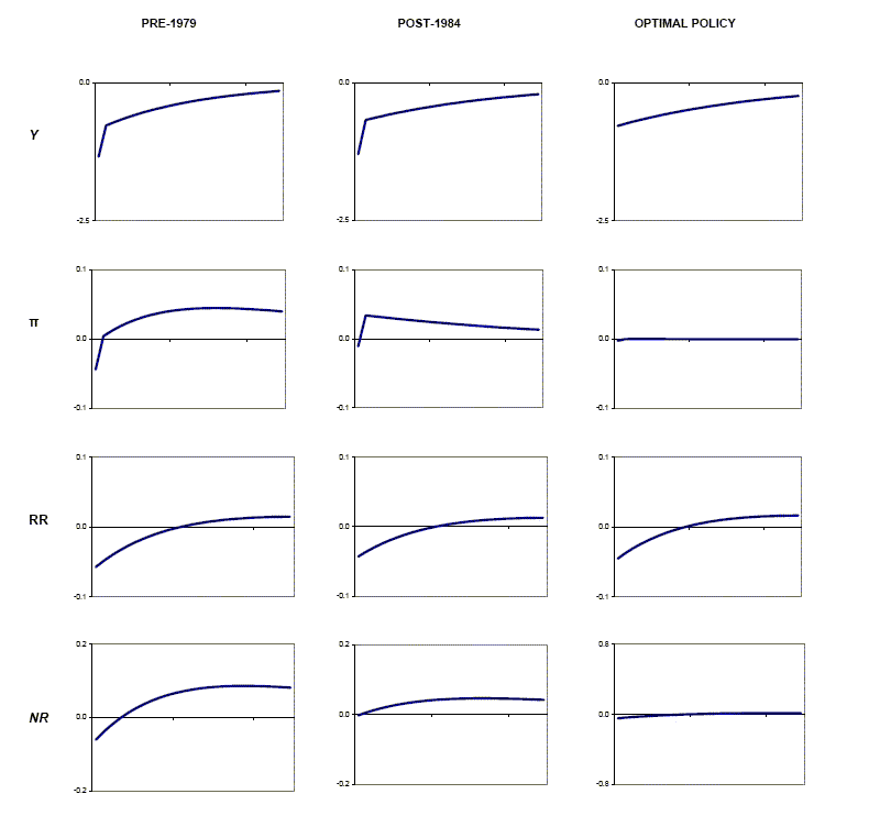
The first two columns report the response of the economy under our benchmark calibration. The interest-rate rules for the pre-1979 and post-1984 period are those estimated by Clarida, Gali, and Gertler (2000). See Table 4 for details. The impulse-responses are plotted for 25 quarters. Y=output, p=inflation, RR=real interest rate, and NR=nominal interest rate.
Data for Figure 4: Responses to a Negative TFP Shock Under Alternative Monetary Policies (in %): Pre-1979
| Output | Inflation | Nominal Interest Rate | Real Interest Rate |
|---|---|---|---|
| -1.339131 | -0.043722 | -0.045427 | -0.057203 |
| -0.774437 | 0.004399 | -0.028881 | -0.048336 |
| -0.719150 | 0.011493 | -0.014310 | -0.040393 |
| -0.667970 | 0.017641 | -0.001525 | -0.033290 |
| -0.620583 | 0.022937 | 0.009650 | -0.026948 |
| -0.576699 | 0.027468 | 0.019373 | -0.021298 |
| -0.536052 | 0.031313 | 0.027788 | -0.016274 |
| -0.498394 | 0.034543 | 0.035028 | -0.011818 |
| -0.463499 | 0.037224 | 0.041211 | -0.007875 |
| -0.431158 | 0.039414 | 0.046447 | -0.004398 |
| -0.401176 | 0.041166 | 0.050834 | -0.001342 |
| -0.373377 | 0.042529 | 0.054462 | 0.001336 |
| -0.347595 | 0.043547 | 0.057412 | 0.003670 |
| -0.323679 | 0.044260 | 0.059758 | 0.005696 |
| -0.301489 | 0.044703 | 0.061567 | 0.007444 |
| -0.280896 | 0.044909 | 0.062900 | 0.008943 |
| -0.261779 | 0.044906 | 0.063811 | 0.010217 |
| -0.244030 | 0.044723 | 0.064350 | 0.011289 |
| -0.227546 | 0.044381 | 0.064563 | 0.012182 |
| -0.212234 | 0.043904 | 0.064489 | 0.012913 |
| -0.198006 | 0.043309 | 0.064165 | 0.013501 |
| -0.184783 | 0.042614 | 0.063624 | 0.013961 |
| -0.172491 | 0.041835 | 0.062895 | 0.014308 |
| -0.161061 | 0.040985 | 0.062006 | 0.014553 |
| -0.150430 | 0.040078 | 0.060979 | 0.014710 |
| -0.140539 | 0.039123 | 0.059838 | 0.014788 |
| -0.131336 | 0.038131 | 0.058600 | 0.014798 |
| -0.122769 | 0.037110 | 0.057282 | 0.014747 |
| -0.114793 | 0.036069 | 0.055901 | 0.014643 |
| -0.107364 | 0.035014 | 0.054470 | 0.014495 |
| -0.100444 | 0.033951 | 0.053001 | 0.014307 |
| -0.093996 | 0.032886 | 0.051504 | 0.014085 |
| -0.087986 | 0.031822 | 0.049990 | 0.013836 |
| -0.082383 | 0.030765 | 0.048466 | 0.013562 |
| -0.077158 | 0.029717 | 0.046939 | 0.013269 |
| -0.072284 | 0.028682 | 0.045417 | 0.012960 |
| -0.067736 | 0.027662 | 0.043905 | 0.012638 |
| -0.063491 | 0.026660 | 0.042407 | 0.012306 |
| -0.059528 | 0.025677 | 0.040929 | 0.011967 |
| -0.055827 | 0.024714 | 0.039472 | 0.011623 |
| -0.052370 | 0.023774 | 0.038041 | 0.011275 |
| -0.049140 | 0.022857 | 0.036638 | 0.010927 |
| -0.046121 | 0.021964 | 0.035265 | 0.010579 |
| -0.043299 | 0.021095 | 0.033924 | 0.010232 |
| -0.040660 | 0.020251 | 0.032616 | 0.009888 |
| -0.038191 | 0.019432 | 0.031342 | 0.009548 |
| -0.035881 | 0.018638 | 0.030103 | 0.009213 |
| -0.033719 | 0.017870 | 0.028900 | 0.008883 |
| -0.031695 | 0.017127 | 0.027732 | 0.008559 |
| -0.029799 | 0.016409 | 0.026601 | 0.008242 |
Data for Figure 4: Responses to a Negative TFP Shock Under Alternative Monetary Policies (in %): Post-1984
| Output | Inflation | Nominal Interest Rate | Real Interest Rate |
|---|---|---|---|
| -1.295011 | -0.010664 | -0.001415 | -0.042850 |
| -0.679706 | 0.033920 | 0.004408 | -0.036190 |
| -0.645915 | 0.032728 | 0.009516 | -0.030195 |
| -0.613800 | 0.031558 | 0.013975 | -0.024810 |
| -0.583278 | 0.030412 | 0.017847 | -0.019979 |
| -0.554270 | 0.029291 | 0.021189 | -0.015654 |
| -0.526702 | 0.028197 | 0.024051 | -0.011791 |
| -0.500502 | 0.027130 | 0.026480 | -0.008348 |
| -0.475603 | 0.026091 | 0.028521 | -0.005287 |
| -0.451940 | 0.025080 | 0.030211 | -0.002574 |
| -0.429452 | 0.024097 | 0.031586 | -0.000178 |
| -0.408080 | 0.023144 | 0.032680 | 0.001932 |
| -0.387770 | 0.022220 | 0.033523 | 0.003781 |
| -0.368469 | 0.021324 | 0.034140 | 0.005394 |
| -0.350127 | 0.020458 | 0.034557 | 0.006794 |
| -0.332697 | 0.019620 | 0.034797 | 0.008001 |
| -0.316132 | 0.018810 | 0.034880 | 0.009033 |
| -0.300391 | 0.018027 | 0.034824 | 0.009908 |
| -0.285432 | 0.017273 | 0.034646 | 0.010642 |
| -0.271217 | 0.016545 | 0.034362 | 0.011248 |
| -0.257709 | 0.015843 | 0.033985 | 0.011741 |
| -0.244873 | 0.015167 | 0.033528 | 0.012130 |
| -0.232674 | 0.014516 | 0.033002 | 0.012429 |
| -0.221083 | 0.013890 | 0.032418 | 0.012645 |
| -0.210068 | 0.013288 | 0.031784 | 0.012789 |
| -0.199602 | 0.012709 | 0.031110 | 0.012869 |
| -0.189655 | 0.012152 | 0.030401 | 0.012892 |
| -0.180204 | 0.011618 | 0.029666 | 0.012864 |
| -0.171224 | 0.011105 | 0.028909 | 0.012792 |
| -0.162690 | 0.010612 | 0.028136 | 0.012682 |
| -0.154581 | 0.010139 | 0.027353 | 0.012538 |
| -0.146875 | 0.009686 | 0.026563 | 0.012366 |
| -0.139554 | 0.009251 | 0.025769 | 0.012168 |
| -0.132596 | 0.008835 | 0.024976 | 0.011949 |
| -0.125986 | 0.008436 | 0.024186 | 0.011713 |
| -0.119704 | 0.008053 | 0.023402 | 0.011462 |
| -0.113735 | 0.007687 | 0.022625 | 0.011198 |
| -0.108064 | 0.007337 | 0.021859 | 0.010925 |
| -0.102675 | 0.007001 | 0.021104 | 0.010645 |
| -0.097554 | 0.006680 | 0.020361 | 0.010359 |
| -0.092689 | 0.006373 | 0.019633 | 0.010069 |
| -0.088066 | 0.006079 | 0.018920 | 0.009777 |
| -0.083673 | 0.005798 | 0.018222 | 0.009484 |
| -0.079499 | 0.005529 | 0.017541 | 0.009191 |
| -0.075534 | 0.005272 | 0.016877 | 0.008899 |
| -0.071765 | 0.005027 | 0.016231 | 0.008610 |
| -0.068185 | 0.004793 | 0.015602 | 0.008323 |
| -0.064783 | 0.004568 | 0.014992 | 0.008040 |
| -0.061551 | 0.004355 | 0.014399 | 0.007762 |
| -0.058480 | 0.004150 | 0.013825 | 0.007488 |
Data for Figure 4: Responses to a Negative TFP Shock Under Alternative Monetary Policies (in %): Optimal Policy
| Output | Inflation | Nominal Interest Rate | Real Interest Rate |
|---|---|---|---|
| -0.782182 | -0.002254 | -0.045160 | -0.045204 |
| -0.742770 | 0.000008 | -0.037049 | -0.037478 |
| -0.705985 | 0.000396 | -0.030272 | -0.030705 |
| -0.672120 | 0.000406 | -0.024307 | -0.024669 |
| -0.640093 | 0.000340 | -0.018993 | -0.019273 |
| -0.609608 | 0.000265 | -0.014251 | -0.014455 |
| -0.580550 | 0.000194 | -0.010025 | -0.010161 |
| -0.552845 | 0.000130 | -0.006269 | -0.006345 |
| -0.526429 | 0.000074 | -0.002939 | -0.002962 |
| -0.501246 | 0.000024 | 0.000002 | 0.000026 |
| -0.477240 | -0.000020 | 0.002592 | 0.002657 |
| -0.454357 | -0.000058 | 0.004862 | 0.004962 |
| -0.432548 | -0.000091 | 0.006842 | 0.006973 |
| -0.411763 | -0.000120 | 0.008560 | 0.008718 |
| -0.391956 | -0.000144 | 0.010041 | 0.010222 |
| -0.373084 | -0.000165 | 0.011308 | 0.011508 |
| -0.355102 | -0.000183 | 0.012382 | 0.012597 |
| -0.337971 | -0.000198 | 0.013282 | 0.013510 |
| -0.321651 | -0.000210 | 0.014026 | 0.014265 |
| -0.306105 | -0.000220 | 0.014629 | 0.014876 |
| -0.291298 | -0.000228 | 0.015106 | 0.015360 |
| -0.277195 | -0.000234 | 0.015471 | 0.015729 |
| -0.263763 | -0.000238 | 0.015735 | 0.015996 |
| -0.250972 | -0.000241 | 0.015910 | 0.016173 |
| -0.238792 | -0.000243 | 0.016006 | 0.016269 |
Footnotes
1. See Kim and Nelson (1999), McConnell and perez-Quiros (2000), and Stock and Watson (2002) Return to text
2. Stock and Watson (2003) investigate counterfactuals in four small macroeconomic models and find that improved monetary policy accounts for less than 10 percent of the decline in output volatility post-1984. The models do suggest, though, that improved policy helps bring down the variance of inflation. Primiceri (2003) estimates a time-varying structural VAR and finds that though the systematic component of monetary policy changed post-1980, the change had a negligible effect on inflation and unemployment Return to text
3. Blanchard and Simon (2001) also argue that the principal reason for a less volatile economy is that it has been hit by smaller shocks. Return to text
4. Schmitt-Grohe and Uribe (2004) and Kollman (2003) examine welfare-maximizing monetary policies in a class of simple, implementable rules in models with endogenous capital accumulation. Our optimal policy analysis does not restrict monetary policy to follow simple Taylor-type rules. Erceg et al. (2000) solve for optimal monetary policy in a model with a fixed aggregate capital stock. Return to text
5. We examine symmetric equilibria. Consequently, it does not matter for the results that household's hold a claim to the dividends of a single firm, rather than to a portfolio of all firms. Return to text
6. We did not specify depreciation
![]() to be a function
of utilization because this tended to lead to model indeterminacy
under our pre-1979 specification for the monetary policy
rule. Return to text
to be a function
of utilization because this tended to lead to model indeterminacy
under our pre-1979 specification for the monetary policy
rule. Return to text
7. We use Matlab's symbolic toolbox to take derivatives of the Lagrangian and then input the resulting analytical first-order conditions into Dynare to solve the model. We also solved the optimal policy problem using a second-order approximation, but found the results to be very similar to those found under the first-order approximation. Return to text
8. Basu et al. (2004) construct a generalized Solow residual that allows for increasing returns, imperfect competition, and variable labor and capital input utilization rates. Their measure is available annually up to 1996. Our constructed TFP series, at an annual frequency, has a correlation of about 0.5 with the BFK measure. The BFK series is a problematic input for our model given that it accounts for, among other things, increasing returns to scale, which the model does not contain. In addition, one might be less confident that an accurate volatility measure can be obtained using annual data for the post-1984 sample, since we would have only 15 observations. For these reasons, we did not input the BFK series into the model. Return to text
9. While our specification of annual price adjustment is common in the literature and close to the findings in Sbordone (2002), it is somewhat longer than the median frequency of price adjustment of 4.3 months reported in Bils and Klenow (2002). We chose the longer duration in part because it allowed us to solve the model under our pre-79 policy rule, in which the coefficient on expected inflation takes a value less than one. Return to text
10. The implied reduced form for inflation takes the form
11. An absence of price-adjustment costs in steady state implies that the Friedman rule is optimal. Since we use a linear algorithm to solve for the optimal monetary policy around the steady state, it would likely be the case that model simulations under optimal policy would violate the zero bound on nominal interest rates. We avoid this problem by assuming a positive price-adjustment cost in steady state. Return to text
12. We use CGG's post-1982 estimates of the policy rule rather than those for the post-1979 period since it lines up more closely with our post-1984 sample. Return to text
13. Orphanides (2004) estimates, using real-time data, that the principal difference between the pre- and post-1979 policy rules is the weight placed on output stabilization, and not the weight placed on inflation. Misperceptions of the size of the output gap coupled with an activist monetary policy would have led to high inflation in the 1970s. See Bullard and Eusepi (2003) for a dynamic, general equilibrium assessment of this view. Return to text
14. Consequently, we do not examine the benefits that accrue from a monetary policy change that eliminates non-fundamental (sunspot) sources of volatility (however, see Boivin and Giannoni (2003) and Lubik and Schorfheide (2004) for investigations along such lines). Although this may be an interesting avenue to explore, it is not clear how to select a particular equilibrium when the equilibrium of the model is locally indeterminate. Return to text
15. Since we use a linear solution method, we do not need to make further distributional assumptions about the oil shock process. Return to text
16. Our minimization criterion for setting the steady state quantity of oil is an equally weighted sum of the deviation of the model-implied standard deviation of output and inflation from their counterparts in the data. Return to text
17. The impulse responses are generated under the benchmark calibration described in section 6, assuming that monetary policy follows the post-1982 rule estimated by Clarida et al. (2000). Return to text
18. We detrend both actual and simulated data using the Hodrick-Prescott filter and calculate standard deviations of the cyclical components. Return to text
19. We do not show the impulse responses to an oil shock under the alternative monetary policies since the overall picture is similar to that of a temporary TFP shock. Return to text
This version is optimized for use by screen readers. Descriptions for all mathematical expressions are provided in LaTex format. A printable pdf version is available. Return to text