
Board of Governors of the Federal Reserve System
International Finance Discussion Papers
Number 905, September 2007--- Screen Reader
Version*
Frequency of Observation and the Estimation
of
Integrated Volatility in Deep and Liquid Financial Markets*
NOTE: International Finance Discussion Papers are preliminary materials circulated to stimulate discussion and critical comment. References in publications to International Finance Discussion Papers (other than an acknowledgment that the writer has had access to unpublished material) should be cleared with the author or authors. Recent IFDPs are available on the Web at http://www.federalreserve.gov/pubs/ifdp/. This paper can be downloaded without charge from the Social Science Research Network electronic library at http://www.ssrn.com/.
Abstract:
Using two newly available ultrahigh-frequency datasets, we investigate empirically how frequently one can sample certain foreign exchange and U.S. Treasury security returns without contaminating estimates of their integrated volatility with market microstructure noise. Using volatility signature plots and a recently-proposed formal decision rule to select the sampling frequency, we find that one can sample FX returns as frequently as once every 15 to 20 seconds without contaminating volatility estimates; bond returns may be sampled as frequently as once every 2 to 3 minutes on days without U.S. macroeconomic announcements, and as frequently as once every 40 seconds on announcement days. With a simple realized kernel estimator, the sampling frequencies can be increased to once every 2 to 5 seconds for FX returns and to about once every 30 to 40 seconds for bond returns. These sampling frequencies, especially in the case of FX returns, are much higher than those often recommended in the empirical literature on realized volatility in equity markets. We suggest that the generally superior depth and liquidity of trading in FX and government bond markets contributes importantly to this difference.
Keywords: Realized volatility, sampling frequency, market microstructure, bond markets, foreign exchange markets, liquidity
JEL classification: C22, G12
1 Introduction
Modeling, measuring, and estimating the volatility of financial asset returns is important for many economic and financial applications, including forecasting and analyzing alternative decisions available to investors and policy makers. One approach to estimating volatility is to use a parametric framework, such as the class of ARCH, GARCH, and stochastic volatility models. If data on returns are available at sufficiently high frequencies, one can also estimate volatility nonparametrically by computing the realized volatility, which is the natural estimator of the ex post integrated volatility. This latter method is appealing both because it is computationally simple and because it is a valid estimator under fairly mild statistical assumptions. In principle, the higher the sampling frequency is, the more precise the estimates of integrated volatility become. In practice, however, the presence of so-called market microstructure features at very high sampling frequencies may create important complications. The finance literature has identified many such features; among them are the fact that financial transactions--and hence price changes and non-zero returns--arrive discretely rather than continuously over time, the fact that buyers and sellers usually face different prices (separated by the bid-ask spread), the presence of negative serial correlation of returns to successive transactions (including the so-called bid-ask bounce), and the price impact of trades. For an overview of many of these market microstructure issues and their importance for financial theory and practice, we refer the reader to, e.g., the books by Hasbrouck (2006), O'Hara (1998), and Campbell et al. (1997, Ch. 3), as well as the journal articles by Roll (1984), Harris (1990, 1991), and Hasbrouck (1991).
The presence of market microstructure features is generally believed to elevate estimates of integrated volatility, especially at the very highest sampling frequencies, relative to the base case of no market microstructure noise. However, this need not always be the case. For example, if an organized stock exchange has designated market makers and specialists, and if these participants are slow in adjusting prices in response to shocks (possibly because the exchange's rules explicitly prohibit them from adjusting prices by larger amounts all at once), it may be the case that realized volatility could drop if it is computed at those sampling frequencies for which this behavior is thought to be relevant.1 In any case, it is widely recognized that market microstructure issues can contaminate estimates of integrated volatility in important ways, especially if the data are sampled at ultra-high frequencies, as is becoming more and more common.
Two different approaches have emerged to dealing with the issue of contamination by market microstructure when estimating integrated volatility. The first approach, which is reportedly the more common one, is simply to sample sufficiently sparsely so that any market microstructure issues should not be a significant concern. This approach is appealing because it permits the use of the intuitive and simple standard realized volatility estimator, and also because it does not require making any assumptions about the nature of the market microstructure noise. However, the choice of sampling frequency is typically somewhat ad hoc, and it could lead to inefficient estimates of integrated volatility if the sampling frequency is chosen too conservatively, i.e., too low. In an attempt to address this concern, Aït-Sahalia et al. (2005) and Bandi and Russell (2006b) have proposed optimal sampling frequency rules that are based on a bias-variance trade-off, viz., between sampling more often and incurring a larger bias and sampling less often and incurring larger variance. Interestingly, whereas much of the early empirical work on estimating integrated volatility was performed using FX market data (e.g., Zhou, 1996, and Andersen, Bollerslev, Diebold, and Labys, 2001), much of the more recent work in this field, especially on the optimal choice of sampling frequency, has been applied to markets for individual stocks (e.g., Bandi and Russell, 2006b, and Hansen and Lunde, 2006).
The second approach is to design alternative estimators of integrated volatility that are less sensitive than the basic realized volatility estimator to the presence of market microstructure noise. This approach, which generally relies on kernel-based or subsampling methods to let researchers use returns sampled at higher frequencies, potentially should allow for a more efficient use of the data. A drawback is that the computation of these estimators may be considerably more complicated than that of the standard realized volatility estimator. Moreover, these more robust estimators may give up some of the standard estimator's appealing simplicity and intuitiveness. These concerns, however, may be overblown in practice. For instance, in this paper we find that a very simple version of a kernel-based estimator can substantially improve upon the performance of the standard estimator, in the sense of permitting the use of much-higher sampling frequencies to estimate integrated volatility without incurring market microstructure-induced bias.
The first aim in the empirical section of our paper is to study, for two specific financial assets, how the standard estimator of integrated volatility is affected by the choice of sampling frequency. The two assets we study are traded in some of the deepest and most liquid financial markets in existence today; they are the spot exchange rate of the dollar/euro currency pair, obtained from Electronic Broking Systems (EBS), and the price of the on-the-run 10-year U.S. Treasury note, traded on BrokerTec. Both of these markets are electronic order book systems, which quite likely represent the future of wholesale financial trading systems. Both markets are strictly inter-dealer. These markets are far larger in terms of total trading volume than markets for individual stocks--even the most liquid handful of stocks traded on the New York Stock Exchange--, and bid-ask spreads are narrower than in typical stock markets. In 2005, bid-ask spreads averaged 1.04 basis points for dollar/euro spot transactions on EBS and 1.68 basis points for 10-year Treasury note transactions on BrokerTec. The two time series are available at ultra-high frequencies--up to the second-by-second frequency.
Our main hypothesis is that, in such deep and liquid markets, market microstructure noise should pose less of a concern for volatility estimation, in the sense that it should be possible to sample returns on such assets more frequently than say, returns on individual stocks, before estimates of integrated volatility encounter significant bias caused by the markets' microstructure features. This thesis is indeed borne out by our empirical work. We show that it is possible to sample the FX data as often as once every 15 to 20 seconds without the standard estimator of integrated volatility showing discernible effects stemming from market microstructure noise. The corresponding sampling interval lengths for returns on 10-year Treasury notes are between 2 and 3 minutes. These intervals are shorter than the sampling intervals of several minutes, usually five or more minutes, that have often been recommended in the empirical literature on estimating integrated volatility for a number of financial markets. These shorter sampling intervals and associated larger sample sizes afford a considerable gain in estimation precision. We conclude that in very deep and liquid markets, microstructure-induced frictions may be much less of an issue for volatility estimation than was previously thought. We also confirm the results of several previous empirical studies that major macroeconomic announcements systematically affect integrated volatility. In addition, we show that the optimal choice of sampling frequency is higher--and the sampling interval lengths are therefore lower--on days with scheduled U.S. macroeconomic announcements.
Although the sampling frequencies at which the standard realized volatility estimator can be used are already very high for the two empirical time series we consider in this paper, it is possible to sample at even higher frequencies by using so-called kernel estimators, which are designed explicitly to control for the effects of market microstructure noise. These estimators can be viewed as the equivalent of so-called robust variance estimators in the traditional time series econometrics literature. We find that by using a very simple version of a kernel estimator, it is possible to sample FX returns at frequencies as high as once every 2 to 5 seconds, and that bond returns can be sampled as frequently as once every 30 to 40 seconds. This estimator, which is almost as easy to compute as the standard realized volatility estimator, thus offers a substantial additional gain in efficiency in terms of how often one can sample on an intraday basis.
Finally, we also examine how certain alternative estimators and measures of daily variation perform for the two time series at hand. These alternative estimators are not based on functions of the standard quadratic variation process, but instead on functions of absolute variation and bipower variation processes. A reason for considering such methods is that they may be more robust than the standard estimator to outlier activity (heavy tails) in the data and, in particular, to jumps that may occur in the price series. In general, these estimators measure somewhat different (but highly relevant) aspects of daily variation than does the standard realized volatility estimator. We find some evidence that these alternative methods are indeed more robust than the standard estimator to the presence of jumps in the returns series. Specifically, estimates of integrated volatility that are based on absolute variation show less dispersion across announcement and non-announcement days than estimates that are based on squared variation. However, we find no evidence that these robust methods are also less sensitive than the standard estimator with regard to bias imparted by market microstructure noise. To the contrary, our results indicate that one should typically sample less frequently when using these robust estimators, relative to the optimal sampling frequency found for the standard volatility estimator.
The remainder of our paper is organized as follows. Section 2 provides some motivation for the use of the standard estimator of integrated volatility, which is based on the quadratic variation of returns. The section also details how market microstructure noise may cause bias in the standard estimator, provides an introduction to kernel-based estimators designed to circumvent this problem, and sets out the use of absolute and bipower variation processes. Section 3 provides an overview of the characteristics of the foreign exchange and bond market data used in our empirical work. Section 4 provides the empirical results for the standard estimator of realized volatility, using volatility signature plots and the Aït-Sahalia et al. (2005) and Bandi and Russell (2006b) rule for choosing sampling frequencies. Section 5 shows the results from the realized kernel estimators. Section 6 provides the estimation results for the robust estimators of realized volatility, such as the one that is based on the absolute variation process. Section 7 provides a discussion of some broader issues raised by our empirical findings, and Section 8 concludes.
2 Motivation and estimation techniques
2.1 Motivation
The fundamental idea behind the use of realized volatility and
high-frequency data is that quadratic variation can be used as a
measure of ex-post variance in a diffusion process. The quadratic
variation ![]() of a process
of a process ![]() is defined as
is defined as
![$\displaystyle QV_{t}=\left[ X,X\right] _{t}=\plim_{n\to\infty}\sum_{j=1} ^{n}\left( X_{t_{j}}-X_{t_{j-1}}\right) ^{2},$](img3.gif)
|
(1) |
for any sequence of partitions
|
(2) |
where
![$\displaystyle \left[ X,X\right] _{t}=\int_{0}^{t}\!\!\!\sigma_{u}^{2}\d u\,.$](img12.gif)
|
(3) |
In this model, which is frequently used in financial economics, the quadratic variation measures the integrated variance over some time interval and is thus a natural way of measuring the ex-post variance. For most of the discussion, and unless otherwise noted, we will maintain the assumption that the logarithm of the price process follows the diffusion process in equation (2). This is not crucial to the analysis in the paper, but it facilitates the exposition of the theoretical concepts outlined below. In Section 2.5 below, we discuss the effects of adding a jump component to equation (2).
Suppose the log-price process ![]() is sampled at
fixed intervals
is sampled at
fixed intervals ![]() over some time
period
over some time
period ![]() . Let
. Let
![]() . The realized
variance, given by
. The realized
variance, given by
|
(4) |
is a natural estimator of the quadratic variation over the interval
![]() . In practice, we usually consider the
integrated volatility, which is the square root of the integrated
variance, and the corresponding realized volatility, which is
obtained by taking the square root of
. In practice, we usually consider the
integrated volatility, which is the square root of the integrated
variance, and the corresponding realized volatility, which is
obtained by taking the square root of ![]() .
.
The properties of ![]() have been analyzed
extensively in the econometrics literature.2 In particular, it
has been shown that under very weak conditions realized variance is
a consistent estimator of quadratic variation. That is, for a fixed
time interval
have been analyzed
extensively in the econometrics literature.2 In particular, it
has been shown that under very weak conditions realized variance is
a consistent estimator of quadratic variation. That is, for a fixed
time interval ![]() ,
,
![]() as
as
![]() . In addition, if
. In addition, if
![]() satisfies equation (2), the limiting
distribution of
satisfies equation (2), the limiting
distribution of ![]() is mixed normal and is
centered on
is mixed normal and is
centered on ![]() :
:
| (5) |
where
![]() is
called the quarticity of
is
called the quarticity of ![]() .
.
2.2 Market microstructure noise
According to the asymptotic result in equation (5), it is
preferable to sample ![]() as frequently as
possible in order to achieve more precise estimates of the
quadratic variation. However, in practice, price changes in
financial assets sampled at very high frequencies are subject to
market frictions--such as the bid-ask bounce and the price impact
of trades--in addition to reacting to more fundamental changes in
the value of the asset. Suppose the observed price
as frequently as
possible in order to achieve more precise estimates of the
quadratic variation. However, in practice, price changes in
financial assets sampled at very high frequencies are subject to
market frictions--such as the bid-ask bounce and the price impact
of trades--in addition to reacting to more fundamental changes in
the value of the asset. Suppose the observed price ![]() can be decomposed as
can be decomposed as
| (6) |
where ![]() is the so-called latent price process
and
is the so-called latent price process
and ![]() represents market microstructure noise.
The object of interest is now the quadratic variation of the
unobserved process
represents market microstructure noise.
The object of interest is now the quadratic variation of the
unobserved process ![]() , which is assumed to
satisfy the diffusion given by equation (2). A standard
assumption is that
, which is assumed to
satisfy the diffusion given by equation (2). A standard
assumption is that ![]() is a white noise
process, independent of
is a white noise
process, independent of ![]() , with mean zero and
constant variance
, with mean zero and
constant variance
![]() . Now, as
. Now, as ![]() ,
the length of sampling intervals, goes to zero, the squared
increments in
,
the length of sampling intervals, goes to zero, the squared
increments in ![]() will be dominated by the
changes in
will be dominated by the
changes in ![]() . This follows because the
increments in
. This follows because the
increments in ![]() are of order
are of order
![]() under
equation (2),
whereas the increments in
under
equation (2),
whereas the increments in ![]() are of
order
are of
order ![]() regardless of sampling
frequency. Calculating the realized variance using extremely high
frequency (such as second-by-second) returns from the observed
price process
regardless of sampling
frequency. Calculating the realized variance using extremely high
frequency (such as second-by-second) returns from the observed
price process ![]() will therefore result in
a biased and inconsistent estimate of the quadratic variation of
the latent price process
will therefore result in
a biased and inconsistent estimate of the quadratic variation of
the latent price process ![]() .
.
2.3 Optimal choice of sampling frequency
The initial reaction to this problem was simply to sample at
frequencies for which market frictions are believed not to play a
significant role. Even with this limitation, daily volatility
estimates can be obtained with some precision. In particular,
sampling prices and returns at the five-minute frequency appears to
have emerged as a popular choice to compute daily-frequency
estimates of volatility. In order to formalize this line of
reasoning, Bandi and Russell (2006b) derive an optimal sampling
frequency rule for the standard realized variance
estimator.3 Their rule is based on a function of
the signal-to-noise ratio between the innovations to the latent
price process and the noise process. Their key assumption is that
by sampling at the highest possible frequency, it may be possible
to obtain a consistent estimate of the variance of the noise,
![]() . For example, let
. For example, let
![]() denote the one-second sampling
frequency, which is the highest possible in our data, and let
denote the one-second sampling
frequency, which is the highest possible in our data, and let
![]() denote the number of
non-zero one-second returns during the day; i.e.,
denote the number of
non-zero one-second returns during the day; i.e.,
![]() counts the number of one-second
periods during the whole day for which there is actual market
activity that moves the price. An estimator of
counts the number of one-second
periods during the whole day for which there is actual market
activity that moves the price. An estimator of
![]() is now given by
is now given by
|
(7) |
where the summation is carried out over the ![]() intervals with nonzero returns. By estimating
intervals with nonzero returns. By estimating
![]() , the strength of the noise in the
returns data can thus be measured. The strength of the signal,
i.e., variations in
, the strength of the noise in the
returns data can thus be measured. The strength of the signal,
i.e., variations in ![]() which come from the
latent price process
which come from the
latent price process ![]() , can be
measured by the quarticity of that process. By relying on data
sampled at a lower frequency, such as once every ten minutes, where
the market microstructure noise should not be an issue, the
quarticity of
, can be
measured by the quarticity of that process. By relying on data
sampled at a lower frequency, such as once every ten minutes, where
the market microstructure noise should not be an issue, the
quarticity of ![]() can be estimated
consistently (though not efficiently) by
can be estimated
consistently (though not efficiently) by
|
(8) |
where
![]() is the number of 10-minute
intervals with non-zero returns in a day. Thus, by using returns
obtained by sampling at different frequencies, it is possible to
assess the relative importance of the signal
is the number of 10-minute
intervals with non-zero returns in a day. Thus, by using returns
obtained by sampling at different frequencies, it is possible to
assess the relative importance of the signal ![]() and the noise
and the noise ![]() . Bandi and
Russell (2006b) show that an approximate rule of thumb for the
optimal sampling frequency,
. Bandi and
Russell (2006b) show that an approximate rule of thumb for the
optimal sampling frequency,
![]() , is
given by
, is
given by
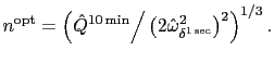
|
(9) |
2.4 Estimators of integrated volatility that are robust to the presence of high-frequency market microstructure noise
The other approach to dealing with the microstructure noise issue is to design estimators that explicitly control for and potentially even eliminate its effects on volatility estimates. At the cost of some loss of simplicity, this approach has the potential of extracting useful information that would otherwise be discarded if a coarser sampling scheme is employed. A number of estimators have been proposed recently to deal with market microstructure noise in this manner; see, for instance, Aït-Sahalia et al. (2005, 2006), Hansen and Lunde (2006), Oomen (2005, 2006), Zhang (2006), and Zhang et al. (2005).4 While these recently-proposed estimators possess several desirable properties, such as asymptotic consistency under their respective maintained assumptions and (in some cases) asymptotic efficiency as well, the actual performance of these estimators in empirical practice remains a topic of ongoing research.
Here, we focus on an estimator proposed by Barndorff-Nielsen, Hansen, Lunde, and Shephard (2006), hereafter BNHLS. Define the realized autocovariation process
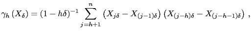
|
(10) |
for ![]() , where the term
, where the term
![]() is a small-sample correction
factor. The realized kernel estimator in BNHLS is given by
is a small-sample correction
factor. The realized kernel estimator in BNHLS is given by
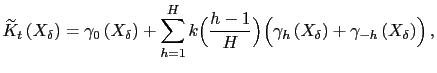
|
(11) |
for some kernel function ![]() satisfying
satisfying
![]() and
and ![]() and for a
suitably chosen lag truncation or bandwidth
parameter
and for a
suitably chosen lag truncation or bandwidth
parameter ![]() .5 The first term in
equation (11),
.5 The first term in
equation (11),
![]() , is
identical to the standard realized variance estimator; the second
term, the weighted sum of autocovariances up to
order
, is
identical to the standard realized variance estimator; the second
term, the weighted sum of autocovariances up to
order ![]() , can thus be viewed as a correction
term which aims to eliminate the serial dependence in returns
induced by microstructure noise. The estimator given in
equation (11)
is obviously a natural analogue of the well-known
heteroskedasticity and autocorrelation consistent (HAC) estimators
of long-run variances in more typical econometric settings.
, can thus be viewed as a correction
term which aims to eliminate the serial dependence in returns
induced by microstructure noise. The estimator given in
equation (11)
is obviously a natural analogue of the well-known
heteroskedasticity and autocorrelation consistent (HAC) estimators
of long-run variances in more typical econometric settings.
Apart from realized kernel estimators, so-called subsampling estimators (e.g., Zhang et al., 2005) have also been proposed to correct for the effects of market microstructure noise. Subsampling estimators are, in fact, very closely related to realized kernel estimators; see Aït-Sahalia et al. (2006), BNHLS, as well as the discussion of the quadratic form representation in Andersen et al. (2006). To keep the empirical exposition below more manageable, we chose to focus only on the kernel approach in this paper. We leave to future research an explicit comparison of the relative performance of kernel estimators and subsampling estimators for the two time series we consider in this paper.
2.5 Absolute power and bipower variation methods
Any estimator that is based on squared values of observations will, to some extent, be sensitive to the occurrence of outliers in the data in general, and, within the framework of financial models, to jumps in asset prices in particular. In the tradition of robust econometric estimation, absolute-value versions of the realized variance estimator have therefore been considered. Barndorff-Nielsen and Shephard (2004b) consider the following normalized versions of realized absolute variation and realized bipower variation. They set
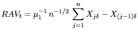
|
(12) |
and
|
(13) |
where
![]() and
and
![]() is a standard normal random variable. In
contrast to the definitions of the realized variance and realized
bipower estimators, it is necessary to use a scaling factor,
is a standard normal random variable. In
contrast to the definitions of the realized variance and realized
bipower estimators, it is necessary to use a scaling factor,
![]() , in equation (12) so that
, in equation (12) so that
![]() converges to a proper limit as
converges to a proper limit as
![]() . The term
. The term
![]() in equation (13) is a
small-sample correction factor.
in equation (13) is a
small-sample correction factor.
In the absence of market microstructure noise and assuming that
equation (2)
holds, Barndorff-Nielsen and Shephard (2004b) show
that ![]() and
and ![]() ,
respectively, are consistent estimators of the quantities
,
respectively, are consistent estimators of the quantities
![]() and
and
![]() . Hence,
realized bipower variation provides an alternative estimator of the
integrated variance of
. Hence,
realized bipower variation provides an alternative estimator of the
integrated variance of ![]() . The usefulness
of realized bipower variation stems from the fact that it has been
shown to provide a consistent estimator of
. The usefulness
of realized bipower variation stems from the fact that it has been
shown to provide a consistent estimator of
![]() under much
more general conditions than realized squared variation does. In
particular, suppose that
under much
more general conditions than realized squared variation does. In
particular, suppose that ![]() exhibits jump
shocks as well as diffusive innovations, such that
exhibits jump
shocks as well as diffusive innovations, such that
|
(14) |
The process ![]() is a jump counting process, which
is assumed to be finite for all
is a jump counting process, which
is assumed to be finite for all ![]() , and the
coefficients
, and the
coefficients ![]() are the sizes of the
associated jumps.6 The quadratic variation of
are the sizes of the
associated jumps.6 The quadratic variation of ![]() is now given by
is now given by
![$\displaystyle \left[ X,X\right] _{t} =\int_{0}^{t}\!\!\! \sigma_{u}^{2} \d u+\sum_{j=1}^{N_{t}} c_{j}^{2} \,,$](img111.gif)
|
(15) |
and the realized variation converges to this term as
![]() . However, the realized
absolute variation and the realized bipower variation are still
consistent estimators of
. However, the realized
absolute variation and the realized bipower variation are still
consistent estimators of
![]() and
and
![]() ,
respectively. By calculating both the realized variation and the
realized bipower variation of
,
respectively. By calculating both the realized variation and the
realized bipower variation of ![]() , one can
separate the total quadratic variation into its continuous and jump
components. This is useful, for instance, in volatility
forecasting, because the jump component of the total quadratic
variation is, in general, far less persistent than the diffusive
component (Andersen et al., 2005).
, one can
separate the total quadratic variation into its continuous and jump
components. This is useful, for instance, in volatility
forecasting, because the jump component of the total quadratic
variation is, in general, far less persistent than the diffusive
component (Andersen et al., 2005).
Even though the limit of the realized absolute variation,
![]() , has no direct
use in most financial applications, such as the pricing of options,
Forsberg and Ghysels (2006) and Ghysels et al. (2006) report
that it is, empirically, a very useful predictor of future
quadratic variation. Since predicting future volatility is
often the ultimate goal, we therefore also discuss in our paper how
often to sample when estimating the absolute variation of the
returns to a financial time series that is obtained from deep and
liquid markets; in particular, we examine how estimates of realized
absolute variation may be affected by market microstructure noise
in such markets. So far, there has been little work aimed at
dealing with the presence of market microstructure noise when
calculating realized absolute and bipower variation. The only
attempt that we are aware of is a paper by Andersen et al.
(2005). They suggest using staggered, or skip-one, returns to
mitigate spurious autocorrelations in the returns that may occur
due to microstructure-induced noise. That is, they suggest using
the following modified version of equation (13),
, has no direct
use in most financial applications, such as the pricing of options,
Forsberg and Ghysels (2006) and Ghysels et al. (2006) report
that it is, empirically, a very useful predictor of future
quadratic variation. Since predicting future volatility is
often the ultimate goal, we therefore also discuss in our paper how
often to sample when estimating the absolute variation of the
returns to a financial time series that is obtained from deep and
liquid markets; in particular, we examine how estimates of realized
absolute variation may be affected by market microstructure noise
in such markets. So far, there has been little work aimed at
dealing with the presence of market microstructure noise when
calculating realized absolute and bipower variation. The only
attempt that we are aware of is a paper by Andersen et al.
(2005). They suggest using staggered, or skip-one, returns to
mitigate spurious autocorrelations in the returns that may occur
due to microstructure-induced noise. That is, they suggest using
the following modified version of equation (13),
|
(16) |
3 The data
3.1 The foreign exchange data
We analyze high-frequency spot dollar/euro exchange rate data from EBS (Electronic Broking System) spanning January through December 2005. EBS operates an electronic limit order book system used by virtually all foreign exchange dealers across the globe to trade in several major currency pairs. Since the late 1990s, inter-dealer trading in the spot dollar/euro exchange rate, the most-traded currency pair, has, on a global basis, become heavily concentrated on EBS. As a result, over our sample period EBS processed a clear majority of the world's inter-dealer transactions in spot dollar/euro. Publicly available estimates of EBS's share of global trading volume in 2005 range from 60% to 90%, and prices on the EBS system were the reference prices used by all dealers to generate FX derivatives prices and spot prices for their customers. Further details on the EBS trading system and the data can be found in Chaboud et al. (2004) and Berger et al. (2005).
The exchange rate data we use are the midpoints of the highest bid and lowest ask quotes in the EBS limit-order book at the top of each second. The exchange rate is expressed as dollars per euro, the market convention. The source of the data is the EBS second-by-second ticker, which is provided to EBS's clients to generate customer quotes and as input for algorithmic trading. These quotes are executable, not just indicative, and they therefore represent a true price series. We consider 5 full 24-hour trading days per week, each one beginning at 17:00 New York time;7 trading occurs around the clock on EBS on those days. We exclude all data collected from Friday 17:00 New York time to Sunday 17:00 New York time from our sample, as trading activity during weekend hours is minimal and is not encouraged by the foreign exchange trading community. We also drop several holidays and days of unusually light trading activity near these holidays in 2005: January 3, Good Friday and Easter Monday, Memorial Day, July 4, Labor Day, Thanksgiving and the following day, December 24-26, and December 30. Similar conventions on holidays have been used in other research on foreign exchange markets, such as by Andersen, Bollerslev, Diebold, and Vega (2003). The resulting number of business days is 251. In the analysis undertaken for this paper, we drop an additional 5 days in order to line up the FX trading days with those in the U.S. bond market, where some additional days are treated as holidays, as described below.
Table 1 presents some summary statistics for dollar/euro returns sampled at 24-hour and 5-minute intervals, where returns are calculated as log-differences of the dollar/euro exchange rate. The mean 24-hour return is about -5 basis points (= -0.05 percent). The standard deviation of the daily returns in 2005 was about 56 basis points (0.56 percent). At the 5-minute frequency, the mean return is, of course, very near zero. In 2005, returns at the 5-minute frequency had a standard deviation of about 3 basis points, and they were extremely leptokurtic.
3.2 The bond data
We analyze high-frequency ten-year on-the-run Treasury cash market data from BrokerTec, also spanning January through December 2005. In the last few years, BrokerTec has become one of the two leading electronic brokers for inter-dealer trading in Treasury securities.8 Estimates of BrokerTec's share of trading in on-the-run Treasury securities in 2005 range from 40 percent to 70 percent. BrokerTec operates an electronic limit order book in which traders can enter bid or offer limit orders (or both) and can also place market orders, similar to EBS .9 We refer our readers to Fleming (2007), Fleming and Rosenberg (2007), and Mizrach and Neely (2006) for discussions of several recent trends in the institutional aspects of trading in U.S. Treasuries. These authors also examine historical factors that underlie the current dominance of electronic trading systems for transacting in on-the-run U.S. Treasury securities.
The ten-year Treasury price data that we use are the mid-point of the highest bid and lowest ask quotes at the top of each second. As in the EBS data, the BrokerTec quotes are executable, not just indicative, and they therefore constitute a true price series. Unlike the EBS data, however, we focus on five 8-hour-long trading days per week, from 08:00 New York time to 16:00 New York time. BrokerTec operates (nearly) continuously on five days each week, from 19:00 New York time to 17:30 New York time, with Monday trading actually beginning on Sunday evening New York time. However, unlike trading in dollar/euro, the vast majority of trading in Treasury securities occurs during New York business hours (Fleming, 1997), and for this reason we limit our analysis to the 08:00 to 16:00 New York time frame. We excluded the same holidays and days of extremely light activity from our sample that we excluded from our EBS data. We also dropped a few additional days, which the U.S. Bond Market Association declared to be market holidays, from the sample.10 The total number of business days retained for the bond data is 246.
Table 2 presents some summary statistics for bond returns sampled at 24-hour and 5-minute intervals, where the bond returns are calculated as log differences of the price of the ten-year on-the-run Treasury note. Daily returns are measured from 16:00 New York time readings. The mean daily price return is about -0.7 basis point (-0.007 percent), as the ten-year Treasury yield changed little on net in 2005. The standard deviation of daily bond returns was about 38 basis points in 2005.11 Returns at the five-minute frequency have a standard deviation of about 3 basis points, and they are also very leptokurtic.
3.3 Range of sample interval lengths and the prevalence of zero-return intervals
The highest available sampling frequency in our datasets is once every second, by construction. In order to have a reasonably large number of samples within each trading day at each frequency we consider, we set the longest sampling interval equal to 30 minutes (1,800 seconds) for the FX returns and to 15 minutes (900 seconds) for bond returns, resulting in within-day sample sizes of 48 and 32, respectively, at the lowest sampling frequencies.
A large fraction of the observed high-frequency returns in both markets under study is equal to zero. A zero return during a given sampling interval can occur either because the price changes during the sampling interval but then returns to its initial level before the interval ends or--much more commonly--because the price does not change at all. Table 3 presents the fraction of sampling intervals with zero returns in both markets, for sampling interval lengths ranging from 1 second to 10 minutes. At the 1-second sampling frequency, about 90 percent of all returns are zero in both series, although the fraction of zero returns is slightly higher for the bond data. At the 1-minute sampling frequency, 45 percent of all bond returns are zero and 26 percent of all exchange rate returns are zero.
Later in this paper, we consider in detail the consequences of the prevalence of sampling intervals with zero returns on the optimal selection of the sampling frequency and on the estimation of integrated volatility using absolute and bipower variation methods.
3.4 U.S. macroeconomic data releases
The impact of scheduled U.S. macroeconomic data releases on the level and volatility of foreign exchange and bond prices has been well documented (e.g., Andersen, Bollerslev, Diebold and Vega, 2003, for foreign exchange, and Fleming and Remolona, 1999, and Balduzzi, Elton, and Green, 2001, for Treasury securities). In parts of the empirical analysis below, we split the full sample into days with certain major U.S. macroeconomic announcements, selected because of their apparent impact on asset prices, and days without announcements. Our chosen monthly scheduled macroeconomic announcements are the employment report (non-farm payrolls and the rate of unemployment), the consumer price index, the producer price index, retail sales, and orders for durable goods. We also select the three quarterly GDP releases (advance, preliminary, final), each released quarterly, and the eight FOMC announcements in 2005. With the exception of the FOMC announcements, which are released at about 14:15 New York time, all announcements considered here are released at 8:30 New York time. Accounting for multiple announcements that occurred on some days in 2005, this gives us a subsample size of 62 days.12 We treat these days as announcement days irrespective of whether the actual data released differed from published market expectations or not.
4 Results for the standard estimator of integrated volatility
4.1 Overview
Figures 1A and 1B show the 2005 time series of daily estimates of the integrated volatility of FX returns and bond returns, based on the standard realized volatility estimator.13 Several conclusions may readily be drawn from these plots. First, for both series there is considerable dispersion in volatility across adjacent days. Second, in 2005 neither volatility series displays a discernible time trend or seasonality pattern, indicating that it may be meaningful to compute (suitably defined) averages in order to study general relationships between sampling frequency and realized volatility. Third, volatility is clearly higher, on average, on days with scheduled major U.S. macroeconomic news announcements, depicted by solid circles in both plots, than on non-announcement days, shown as open squares. This is particularly--but certainly not surprisingly--true for the bond return volatility estimates shown in Figure 1B.
A volatility signature plot, by common convention, graphs sampling frequencies on the horizontal axis and the associated estimates of realized volatility on the vertical axis. Such plots, which appear to have been first used in the context of realized volatility estimation by Andersen et al. (2000), are now used frequently in empirical research on this subject, as they provide an intuitive visual tool for the analysis of the relationships between these two variables. Quite often, it is possible to discern from a volatility signature plot a sampling frequency, which we label the critical sampling frequency, that serves to separate sufficiently-low frequencies (longer sample intervals), for which market microstructure noise does not seem to affect estimates of integrated volatility, from the higher frequencies (shorter sample intervals), for which market microstructure noise does appear to have an effect. We make extensive use of volatility signature plots in our paper. Because of the need to display a very wide range of sampling frequencies in this paper, and because our focus is on the empirical effects of market microstructure noise--which are generally thought to be present in returns only at the higher sampling frequencies--we display the signature plots using a base-2 logarithmic scale on the horizontal axis rather than the standard, i.e., linear scale. The use of a logarithmic scale, by design, gives much more visual prominence to any changes in volatility for the shorter-length sampling intervals (higher sampling frequencies).
We note that the shapes of the daily volatility signature plots can vary considerably across days. Figures 2A, 2B, and 2C show signature plots for FX volatility for three days in 2005: October 3, an average volatility day; July 21, a day of very high volatility;14 and October 18, a day of slightly below-average volatility. It is immediately apparent that these signature plots differ not only in the ranges of their vertical scales but also in their shapes. On October 3 (Figure 2A), realized volatility decreases at first as the sampling interval lengths increase from 1 second to about 15 or 20 seconds, and then shows no further overall trend but a rapidly increasing dispersion as the lengths of the sampling intervals increase further all the way out to 30 minutes (1,800 seconds). On July 21, in contrast, the plot line at first declines slightly as the sampling interval length rises from 1 second to 3 seconds, but then increases on average (and also becomes much more dispersed) as the interval lengths increase further. Yet another pattern prevailed on October 18: the realized volatility at first decreases nearly monotonically as the sampling interval lengths rise from 1 second to about 20 seconds, then is roughly constant as the interval lengths increase to about 4 minutes (240 seconds), and declines once again as the interval lengths rise even more.
Considerable variation in the shape of the dependence of realized volatility on sampling frequency is also evident for bond returns for these three days. On October 3 (Figure 3A), the plot line at first decreases steadily up to a sample length of about 30 seconds, and then becomes quite dispersed for longer sampling intervals. Even though July 21 was not a day with a scheduled major macroeconomic news release, as defined in section 3.4, it was a day with far-above average volatility in bond markets as well, in part because of some spillover from the busy day in FX markets, but also because former Federal Reserve Chairman Greenspan presented a part of the FOMC's semiannual monetary policy report that day. For this day (Figure 3B), realized volatility declines (almost) monotonically as the sample length increases. Finally, on October 18 (Figure 3C), the plot line at first declines sharply until returns are sampled every 30 seconds or so, and settles into a wide range of estimated volatilities for longer sampling intervals.
4.2 The dependence of realized volatility on the sampling frequency
As we noted in the discussion of Figure 1, the realized volatility of FX and bond returns is higher on average on days with scheduled major U.S. macroeconomic news announcements. This result is especially evident when one averages the volatility estimates over time, i.e., if the volatility signature curves are averaged separately for announcement days and non-announcement days.
Figure 4A shows the effect of averaging within each of these two types of days on the relationship between sampling frequency and realized volatility for dollar/euro returns. The plot highlights the stylized fact that if a day falls into the subset of announcement days, realized volatility is elevated relative to the subset of non-announcement days. In addition, the figure also shows that, on average, estimates of realized volatility on non-announcement days are quite insensitive to the choice of sampling interval length, at least as long as it falls into a range from about 20 seconds to about 10 minutes. In contrast, for sampling intervals shorter than 20 seconds, the estimates of integrated volatility are noticeably higher, and they increase progressively as the interval lengths decrease. This suggests that whereas market microstructure noise is present and affects realized volatility at the very highest sampling frequencies, it does not have a noticeable effect on realized volatility for sampling frequencies lower than once every 20 seconds. This same general finding also applies for the subset of days with major scheduled economic announcements: realized volatility increases markedly if returns are sampled more often than once every 15 seconds.15 Note that for the case of FX returns, the critical sampling frequencies, i.e., the frequencies above which market microstructure noise has an increasingly important impact on realized volatility, are roughly the same in the two subsamples.
Figure 4B shows the time-averaged signature plots of bond returns for announcement days and for non-announcement days. One notes immediately that, for any given sampling frequency, integrated volatility is much higher on announcement days than it is on non-announcement days. In addition, it appears that, on average, the contribution of market microstructure noise to realized volatility is considerably larger for bond returns, as the slopes of the (time-averaged) signature plots are steeper at the very highest sampling frequencies than was the case for FX returns. Third, and of the most relevance for the purposes of our paper, the critical sampling frequency is rather different from the FX case, for both announcement and non-announcement days. It is in the range of once every 120 to 180 seconds on days without scheduled major macroeconomic announcements, and about once every 40 seconds on announcement days. We infer that even though volatility is higher on announcements days, the critical sampling frequency is at least three times higher on announcement days than on non-announcement days. This finding clearly suggests that it is preferable to sample bond returns more frequently on announcement days than on non-announcement days, in order to obtain volatility estimates that are more precise yet not affected noticeably by market microstructure noise.
To sum up, when using the standard realized volatility estimator, the signature plots suggest that it is possible to sample FX returns as frequently as once every 20 seconds on non-announcement days (15 seconds on announcement days), and to sample bond returns as often as once every 2 to 3 minutes on non-announcement days (once every 40 seconds on announcement days), without incurring a significant penalty in the form of an upward bias to estimated volatility. Our findings regarding the critical sampling frequency for volatility estimation for FX returns are quite different from those reported by other researchers, who have typically focused on returns to individual equities and have suggested that one should not sample more often than once every 5 minutes or so if one wishes to avoid bias caused by market microstructure dynamics (e.g., Andersen, Bollerslev, Diebold, and Ebens, 2001).
We have already noted that there is considerable variability in the shapes of the daily volatility signature plots, and that some of this variability appears to be associated with the arrival of macroeconomic news. To illustrate that there is considerable variability in the shapes of the signature plots even within the subset of just the non-announcement days, we show the median, the first and third quartiles, and the 5th and 95th percentiles of the distribution of realized volatility estimates, computed from non-announcement days only. To simplify the exposition, we show these quantiles (see Figure 5A for FX and 5B for bonds) standardized by the average of each day's volatility estimates for 9 sampling frequencies in the 4 minute to 6 minute range. For FX returns (Figure 5A), one can again note the wide array of sampling interval lengths, from about 20 seconds to about 10 minutes, for which the median standardized volatility estimate is remarkably insensitive to the choice of sampling frequency. The interquartile range and the 90-percent confidence band become increasingly wider as the sampling frequency moves away from the 4 to 6 minute range. But even at sampling frequencies in the 4 to 6 minute range, one notes that the widths of both the interquartile range and the 90-percent confidence band are not close to zero. This shows that estimates of realized volatility can be quite sensitive to the precise choice of sampling frequency even when these sampling frequencies are very close to each other.
The analogous graph for bond returns, Figure 5B, is qualitatively similar to Figure 5A, but it differs from the FX case in two important ways (in addition to the already-noted narrower range of frequencies, over which the median normalized volatility estimate is close to 1). First, at the 1-second frequency, the median volatility estimate is more than three times larger than the 4-to-6 minute average median estimate. Second, the confidence intervals widen out even more quickly as the sampling intervals move away from the 4-to-6 minute range. Thus, bond return volatility estimates are not only affected more strongly by market microstructure effects than FX returns are, but their heterogeneity is also far larger. We discuss some of the consequences of these observations for applied work in Section 7.
4.3 A formal rule for choosing the optimal sampling frequency
In addition to examining volatility signature plots, one may wish to have a more formal method for establishing the critical sampling frequency. One such method is the optimal sampling rule of Bandi and Russell (2006b), which was introduced in Section 2 and is also very similar to the rule developed by Aït-Sahalia et al. (2005). The optimal sampling frequencies for each day of the sample, based on equation (9), are shown in Figures 6A and 6B. The average sample interval lengths across all days in the full sample are 170 and 310 seconds, respectively, for FX returns and bond returns. Although there is a fair degree of variation from day to day, these averages are nevertheless considerably above those we deduced from the volatility signature plots shown in the previous section. This is especially true for the FX returns.
Signature plots are, of course, informal graphical tools which
cannot by themselves deliver unambiguous answers. Nevertheless,
signature plots are essentially model-free and they rely on much
less stringent assumptions about the nature of the data generating
process than the formal sampling rule. For example, Bandi and
Russell (2006b) assume that there are no jumps in the price
process. Moreover, it is also possible that the variance
![]() of the noise term cannot be
estimated sufficiently accurately from the returns sampled at the
second-by-second frequency, which is the highest-available
frequency in both datasets. Recall that, according to the signature
plots, it may be possible to sample as often as once every 15
to 20 seconds in the FX market without incurring a significant
bias caused by market microstructure features. It may well be the
case that returns sampled at the one-second frequency still contain
too much signal--and hence not enough noise--in order to be able to
estimate
of the noise term cannot be
estimated sufficiently accurately from the returns sampled at the
second-by-second frequency, which is the highest-available
frequency in both datasets. Recall that, according to the signature
plots, it may be possible to sample as often as once every 15
to 20 seconds in the FX market without incurring a significant
bias caused by market microstructure features. It may well be the
case that returns sampled at the one-second frequency still contain
too much signal--and hence not enough noise--in order to be able to
estimate
![]() consistently; Hansen and Lunde
(2006) make a similar point. This issue may be less of a problem
for the bond returns, where the signature plots had indicated
critical sampling intervals in the 2 to 3 minute range. This may
explain why the results from the signature plots and the
Bandi-Russell sampling rule are somewhat closer to each other for
bond returns than they are for FX returns.
consistently; Hansen and Lunde
(2006) make a similar point. This issue may be less of a problem
for the bond returns, where the signature plots had indicated
critical sampling intervals in the 2 to 3 minute range. This may
explain why the results from the signature plots and the
Bandi-Russell sampling rule are somewhat closer to each other for
bond returns than they are for FX returns.
It is interesting to note that the optimal sampling frequencies obtained using the Bandi and Russell rule are higher, i.e., the implied sampling interval lengths are shorter, on days with scheduled major macro announcements. This confirms one of the findings we obtained from the signature plots, which is that even though market microstructure noise is likely to be greater on announcement days (for instance, in terms of a larger bid-ask spread), the signal is even stronger on such days, implying that returns can be sampled more frequently on announcement days.
As was noted in Section 3.3, when returns
are sampled at very high frequencies, many of the FX and bond
returns are zero because there is no price change over many of the
short time intervals. Phillips and Yu (2006a and 2006b) note that
the prevalence of flat pricing over short time intervals implies
that the market microstructure noise and the unobserved efficient
price components of the observed price process are negatively
correlated over these periods, and that these two components may
become perfectly negatively correlated as
![]() . Put differently, the
maintained assumption that the market microstructure noise is
independent of the latent price process, which underlies the
derivation of the Bandi and Russell rule, cannot be strictly valid
if the observed price process is discrete rather than continuous.
In such a framework, sampling at ever-higher frequencies ultimately
does not even produce a consistent estimator of the variance of the
market microstructure noise. If this feature of the data is not
taken into account, the Bandi and Russell rule will tend to lead to
choices of the optimal sampling interval lengths that are too
large. We interpret our empirical results as being fully consistent
with this theoretical observation.
. Put differently, the
maintained assumption that the market microstructure noise is
independent of the latent price process, which underlies the
derivation of the Bandi and Russell rule, cannot be strictly valid
if the observed price process is discrete rather than continuous.
In such a framework, sampling at ever-higher frequencies ultimately
does not even produce a consistent estimator of the variance of the
market microstructure noise. If this feature of the data is not
taken into account, the Bandi and Russell rule will tend to lead to
choices of the optimal sampling interval lengths that are too
large. We interpret our empirical results as being fully consistent
with this theoretical observation.
5 Kernel-based methods
5.1 Autocorrelations in high-frequency returns
The use of the realized kernel estimator of integrated volatility, described in Section 2.4 above, is motivated along lines similar to those for heteroskedasticity and autocorrelation consistent (HAC) estimators of the long-run variance of a time series in traditional econometrics (e.g., Newey and West, 1987). That is, by adding autocovariance terms, an estimator is constructed which better captures the relevant "long-run" variance in the data. Before showing our empirical results for the performance of the BHNLS realized kernel estimator, it is therefore instructive to study the autocorrelation patterns in the high-frequency intraday returns data to build up some intuition that will help guide the interpretation of our empirical results.
Figure 7A shows the average autocorrelation across all days in the FX returns, out to 30 lags, for data sampled at the 1, 10, 30, and 60-second sampling frequencies. That is, for a given lag and sampling frequency, the within-day autocorrelation in high-frequency returns is calculated for each day and is then averaged across all days in the sample. The corresponding results for the bond returns are shown in Figure 7B. When sampling at the 1-second frequency, it is evident that there is some negative autocorrelation in the returns, and that this correlation stretches out for about 10 to 15 lags, i.e., that non-zero serial dependence in 1-second returns persists for about 10 to 15 seconds. For returns sampled at the 10-second frequency, there is still some evidence of negative autocorrelation at the first 2 lags in the FX returns and in the first 4 to 5 lags in the bond returns. For returns sampled at the 30- and 60-second frequencies, there is little evidence of any systematic pattern in the autocorrelations of the FX returns; for the bond returns, only the first two serial correlation coefficients are nonzero for these two sampling frequencies.
The autocorrelation patterns shown in Figure 7 correspond well to the findings using signature plots of how often one can sample returns when using the standard realized volatility estimator. In particular, there is little evidence of any autocorrelation in the FX data for returns sampled at frequencies lower than once every ten seconds. The conclusion from the volatility signature plots shown above was that the critical sampling frequency for FX returns is in the 15 to 20 second range. This finding corresponds very well to the fact that FX return autocorrelations are insignificant for time spans beyond about 20 seconds. Similarly, because there is still a large amount of negative first-order autocorrelation in the one-minute bond returns, it is not surprising that we also obtained a much lower critical sampling frequency for this asset using the signature plot method.
Overall, the results in Figure 7 suggest that in the case of FX returns and for sampling interval lengths shorter than 30 seconds, using kernel estimators should help reduce any bias in realized volatility estimates. For the bond returns, the same would seem to hold for returns sampled at frequencies higher than once every 2 minutes.
5.2 Optimal bandwidth choice
The graphs in Figure 7 give some indication of how many lags one
may want to include in the realized kernel estimator in
equation (11).
However, they do not, by themselves, provide a simple prescription
for action. BNHLS also propose a rule for an optimal choice of the
bandwidth or lag truncation parameter. They show that, in their
framework, the optimal bandwidth is a function of both the sampling
frequency and a scale parameter, ![]() , which is
independent of the sampling frequency;
, which is
independent of the sampling frequency; ![]() must
be estimated, and the details are given in BNHLS. The optimal
bandwidth is then given by
must
be estimated, and the details are given in BNHLS. The optimal
bandwidth is then given by
![]() , although for very high
sampling frequencies (and hence for very large values
of
, although for very high
sampling frequencies (and hence for very large values
of ![]() ) BNHLS recommend setting
) BNHLS recommend setting
![]() . We use this latter
formula for sampling intervals shorter than 30 seconds.
. We use this latter
formula for sampling intervals shorter than 30 seconds.
The time series of optimal bandwidths in 2005 for returns sampled at the 1-second frequency are shown in Figure 8. For FX data (Figure 8A), the optimal bandwidths range between 4 and 7, and for bond returns (Figure 8B), the optimal bandwidths are typically between 6 and 10. There seems to be little systematic variation between announcement and non-announcement days. The optimal bandwidths are roughly similar to, but usually somewhat smaller, than the number of lags for which there seems to be a non-zero autocorrelation in the 1-second returns (Figure 7). As with any kernel estimator, the choice of the value for the bandwidth parameter involves a bias-variance trade-off, with a larger value leading to a smaller bias but also a higher variance. The optimal bandwidth choice incorporates this bias-variance trade-off. It is, in general, not optimal to control for all of the autocorrelation in the data by using a very large value for the bandwidth parameter, as doing so may induce a lot of variance into the estimator.
Calculating the optimal bandwidth parameter ![]() for returns sampled at the 1-minute and lower frequencies, we find
that the result is always a number between 0 and 1, for
both financial asset returns series and for all days in the sample.
Depending on whether one rounds the results up or down--recall that
the bandwidth has to be an integer--the result is thus always an
optimal bandwidth of either 0 or 1 for these lower
sampling frequencies. In fact, all of the optimal bandwidths are
less than
for returns sampled at the 1-minute and lower frequencies, we find
that the result is always a number between 0 and 1, for
both financial asset returns series and for all days in the sample.
Depending on whether one rounds the results up or down--recall that
the bandwidth has to be an integer--the result is thus always an
optimal bandwidth of either 0 or 1 for these lower
sampling frequencies. In fact, all of the optimal bandwidths are
less than ![]() , so that simple rounding would
yield 0 as the optimal number of lags in
equation (11)
for sampling frequencies equal to or less than once a minute.
Throughout the rest of the analysis reported in this section, the
estimate for the optimal bandwidth is always rounded up, so that at
least one lag is always included in the realized kernel estimator
that incorporates the optimally chosen bandwidth for each sampling
frequency.
, so that simple rounding would
yield 0 as the optimal number of lags in
equation (11)
for sampling frequencies equal to or less than once a minute.
Throughout the rest of the analysis reported in this section, the
estimate for the optimal bandwidth is always rounded up, so that at
least one lag is always included in the realized kernel estimator
that incorporates the optimally chosen bandwidth for each sampling
frequency.
In summary, for the very highest sampling frequencies available in our dataset, the bandwidth selection rules of BNHLS suggest that a moderate number of lags should be included, but for lower sampling frequencies the rule indicates that at most one lag should be included.
5.3 Signature plots for realized kernel estimates
In this section we display signature plots for 6 different
choices of ![]() : the standard realized volatility
estimator (which corresponds to the realized kernel estimator with
bandwidth zero), the realized kernel estimator with fixed
bandwidths of 1, 5, 10, and 30, and the realized kernel
estimator that uses a bandwidth optimally chosen for each sampling
frequency.
: the standard realized volatility
estimator (which corresponds to the realized kernel estimator with
bandwidth zero), the realized kernel estimator with fixed
bandwidths of 1, 5, 10, and 30, and the realized kernel
estimator that uses a bandwidth optimally chosen for each sampling
frequency.
As we did in Section 4 for the standard
realized volatility estimator, we begin by studying the volatility
signature plots for three specific business days in 2005.
Signature plots for FX returns on these days are displayed in
Figure 9, while signature plots for bond returns are shown in
Figure 10. Figure 9A shows the signature plot of FX
returns on October 4, 2005, which was a day of average
volatility. For this day, we easily observe the pattern that one
would expect as a result of changing the bandwidth parameter. The
standard estimator, which is obtained by setting ![]() , yields nearly constant estimates of realized volatility
(of about 8.5 percent at an annualized rate) for all sampling
interval lengths between about 15 seconds and about 4 minutes; in
contrast, for sampling frequencies higher than about once every 15
seconds the standard estimator is biased upwards, and it becomes
increasingly more biased as the sampling frequency increases. For
bandwidths greater than 0, the influence of market
microstructure noise on realized volatility becomes increasingly
less pronounced, especially at the highest-available sampling
frequencies. For
, yields nearly constant estimates of realized volatility
(of about 8.5 percent at an annualized rate) for all sampling
interval lengths between about 15 seconds and about 4 minutes; in
contrast, for sampling frequencies higher than about once every 15
seconds the standard estimator is biased upwards, and it becomes
increasingly more biased as the sampling frequency increases. For
bandwidths greater than 0, the influence of market
microstructure noise on realized volatility becomes increasingly
less pronounced, especially at the highest-available sampling
frequencies. For ![]() (the blue short-dashed line), we
find that one can sample as frequently as once every 5 seconds
without incurring any apparent bias in estimated volatility;
setting
(the blue short-dashed line), we
find that one can sample as frequently as once every 5 seconds
without incurring any apparent bias in estimated volatility;
setting ![]() would allow us to sample as frequently
as once every 2 seconds; and if one were to use 30 lags in the
kernel estimator, there is no apparent bias even at the 1-second
sampling frequency. Using the optimal bandwidth produces a
signature plot that is quite similar to the one that results from
using a fixed bandwidth equal to 1.
would allow us to sample as frequently
as once every 2 seconds; and if one were to use 30 lags in the
kernel estimator, there is no apparent bias even at the 1-second
sampling frequency. Using the optimal bandwidth produces a
signature plot that is quite similar to the one that results from
using a fixed bandwidth equal to 1.
Our findings regarding the effects of varying ![]() on realized kernel estimates of volatility are very similar
for October 18, 2005, which was a low-volatility day; see
Figure 9C. In contrast, for the high-volatility day of July
21, 2005, shown in Figure 9B, it is harder to draw any firm
conclusions. On that day, using a value of
on realized kernel estimates of volatility are very similar
for October 18, 2005, which was a low-volatility day; see
Figure 9C. In contrast, for the high-volatility day of July
21, 2005, shown in Figure 9B, it is harder to draw any firm
conclusions. On that day, using a value of ![]() would result in estimates of realized volatility that are actually
slightly larger than those obtained with the standard
estimator, except when the sampling interval lengths are as short
as 1 or 2 seconds. It is worth noting that volatility and
trading volume were both exceptionally high on that day, and hence
it may not even be necessary to employ a kernel-based correction
for this specific day in order to obtain a low-bias estimate of
volatility.
would result in estimates of realized volatility that are actually
slightly larger than those obtained with the standard
estimator, except when the sampling interval lengths are as short
as 1 or 2 seconds. It is worth noting that volatility and
trading volume were both exceptionally high on that day, and hence
it may not even be necessary to employ a kernel-based correction
for this specific day in order to obtain a low-bias estimate of
volatility.
The results for the bond returns on the same three dates are
overall quite similar to those for FX returns, but there are also
some striking differences. In Figure 10A, for the medium-volatility
day of October 5, 2005, we see a pattern that is fairly similar to
the one we observed in Figure 9A for FX returns: setting
![]() already achieves important gains in
terms of the usable critical sampling frequency, from about once
every 20 seconds to once every 4 seconds; by
already achieves important gains in
terms of the usable critical sampling frequency, from about once
every 20 seconds to once every 4 seconds; by ![]() , one can sample as frequently as once every second; and
increasing the bandwidth further to
, one can sample as frequently as once every second; and
increasing the bandwidth further to ![]() produces
little additional gain for any of the higher sampling frequencies
of interest.16 For July 21, 2005, setting
produces
little additional gain for any of the higher sampling frequencies
of interest.16 For July 21, 2005, setting
![]() shortens the critical sampling interval
length from about 2 minutes to about 30 seconds, and setting
shortens the critical sampling interval
length from about 2 minutes to about 30 seconds, and setting
![]() or
or ![]() reduces the
length of this interval further, to about 15 seconds. The patterns
for the low-volatility day of October 18, 2005, shown in
Figure 10C, also suggest that setting
reduces the
length of this interval further, to about 15 seconds. The patterns
for the low-volatility day of October 18, 2005, shown in
Figure 10C, also suggest that setting ![]() or
or
![]() achieves significant gains in terms of
the achievable critical sampling frequency, raising it to about
once every 4 to 8 seconds.
achieves significant gains in terms of
the achievable critical sampling frequency, raising it to about
once every 4 to 8 seconds.
Figure 11 shows the signature plots of FX returns averaged
separately for non-announcement days and announcement days in 2005.
As was discussed in Section 4, when using the
standard realized volatility estimator the critical sampling
interval length for FX returns on non-announcement days and
announcement days, respectively, was between 15 and 20 seconds in
2005. By including just one lag in the realized kernel estimator,
the critical sampling interval length for FX returns drops to about
4 seconds (on average) on non-announcement days. Using the optimal
bandwidth selection rule of BHNLS results in a similar critical
sampling interval length. If one sets ![]() or
or
![]() , even sampling at the 1-second
frequency seems admissible for the purpose of calculating realized
volatility. On the subset of announcement days, shown in the lower
panel of Figure 11, setting
, even sampling at the 1-second
frequency seems admissible for the purpose of calculating realized
volatility. On the subset of announcement days, shown in the lower
panel of Figure 11, setting ![]() shortens the
critical sampling interval length to about 8 seconds, and setting
shortens the
critical sampling interval length to about 8 seconds, and setting
![]() shortens this interval still further, to
about 4 seconds. The results for the bond returns, shown in
Figure 12, are similar in nature to those for FX returns.
Whereas the critical sampling frequency for the standard estimator
of realized volatility on non-announcement days is between once
every 2 to 3 minutes, including just 1 lag in the realized
kernel estimator increases the critical sampling frequency to about
once every 40 seconds on non-announcement days and once every 30
seconds on announcement days; using 30 lags, this frequency climbs
to about once every 8 seconds, on both types of days in 2005.
shortens this interval still further, to
about 4 seconds. The results for the bond returns, shown in
Figure 12, are similar in nature to those for FX returns.
Whereas the critical sampling frequency for the standard estimator
of realized volatility on non-announcement days is between once
every 2 to 3 minutes, including just 1 lag in the realized
kernel estimator increases the critical sampling frequency to about
once every 40 seconds on non-announcement days and once every 30
seconds on announcement days; using 30 lags, this frequency climbs
to about once every 8 seconds, on both types of days in 2005.
5.4 Implications for practical use of realized kernel estimators
The results just presented indicate that there is considerable
scope for achieving much higher critical sampling frequencies, for
FX and bond returns, by using a kernel estimator rather than the
standard estimator of realized volatility, and thereby also
achieving greater precision in the estimates of volatility. There
is, however, a bias-variance trade off for the number of lags
included in the realized kernel estimator. Thus, even though we
find that using 30 lags would allow us to sample at the 1-second
frequency in the case of FX returns and the 8-second frequency for
bond returns, it may not be optimal to do so. Indeed, according to
the BNHLS rule, the (time-averaged) optimal bandwidth at the
1-second frequency is always much smaller than 30. Using the
optimal bandwidth, the critical sampling frequency appears to be
about once every 2 to 5 seconds for FX returns, while for bond
returns it is about once every 30 to 40 seconds.
Unfortunately, calculating the optimal bandwidth is fairly
complicated. However, judging by the results shown in
Figures 9, 10, 11, and 12, our empirical results for the
kernel-based realized volatility estimator using the optimally
chosen bandwidth are very similar for those we found using the
kernel estimator with a fixed lag length of 1. Note that for
![]() the kernel estimator has a very simple
functional form, viz.
the kernel estimator has a very simple
functional form, viz.
| (17) |
because if ![]() we have
we have ![]() in
equation (11).
Therefore, at least for the two financial returns series studied in
this paper, we find that by augmenting the standard realized
volatility estimator with just one additional term, the critical
sampling frequency can be increased considerably without giving up
much in terms of the simplicity of the calculations. This estimator
is, incidentally, also identical to the noise-corrected estimator
proposed in the seminal paper of Zhou (1996).
in
equation (11).
Therefore, at least for the two financial returns series studied in
this paper, we find that by augmenting the standard realized
volatility estimator with just one additional term, the critical
sampling frequency can be increased considerably without giving up
much in terms of the simplicity of the calculations. This estimator
is, incidentally, also identical to the noise-corrected estimator
proposed in the seminal paper of Zhou (1996).
6 Estimation of integrated volatility using absolute power and bipower variation methods
The standard estimator of integrated volatility is potentially quite sensitive to outliers, as it is computed from squared returns. This raises the issue of how robust estimators of volatility, which are functions of absolute rather than squared returns, perform in practice. As discussed before, these estimators converge to measures of the daily variation of the diffusive , or non-jump, part of the returns process. Since much of the difference in daily volatility that was seen for announcement days relative to non-announcement days (Figure 4), may very well stem from jumps rather than diffusive moves in returns, it is particularly interesting to examine how estimates of volatility differ between announcement and non-announcement days when the two robust methods are used. In addition, we also study the degree to which market microstructure noise affects estimates of volatility across sampling frequencies when robust estimators are employed.
6.1 Volatility estimation using absolute variation methods
The realized absolute variation of a continuous time diffusion
process ![]() , sampled over
, sampled over ![]() at
intervals
at
intervals ![]() , was introduced earlier as
, was introduced earlier as
|
(18) |
The factor
![]() is needed to obtain an estimate
of the mean absolute variation of
is needed to obtain an estimate
of the mean absolute variation of ![]() over
over
![]() ,
,
![]() , under the
diffusion model (2),
rather than of the average absolute return of
, under the
diffusion model (2),
rather than of the average absolute return of ![]() over that period.17 Because a diffusion process has
unbounded absolute variation, scaling by
over that period.17 Because a diffusion process has
unbounded absolute variation, scaling by ![]() is required to obtain an estimator that converges to
a proper limit as the sample size,
is required to obtain an estimator that converges to
a proper limit as the sample size, ![]() , increases
to infinity. Because real data are generated discretely and not
continuously, the term sample size needs to be interpreted
carefully in empirical work. When data are generated discretely,
there will be time intervals during which no new data arrive and
hence returns are zero. Furthermore, the relative frequency of
zero-return intervals increases as sampling frequency
rises.18 With discretely-generated data,
then, one must take care not to use the theoretical sample size,
, increases
to infinity. Because real data are generated discretely and not
continuously, the term sample size needs to be interpreted
carefully in empirical work. When data are generated discretely,
there will be time intervals during which no new data arrive and
hence returns are zero. Furthermore, the relative frequency of
zero-return intervals increases as sampling frequency
rises.18 With discretely-generated data,
then, one must take care not to use the theoretical sample size,
![]() , that corresponds to
a given sampling interval length
, that corresponds to
a given sampling interval length ![]() , as
more and more of the sample periods will be characterized by zero
returns as
, as
more and more of the sample periods will be characterized by zero
returns as
![]() . Instead, one must use
the effective sample size, i.e., the number of intervals within a
day during which a transaction occurred.
. Instead, one must use
the effective sample size, i.e., the number of intervals within a
day during which a transaction occurred.
We compute estimates of the daily variation based on the realized absolute variation of FX and bond returns using the same range of sampling frequencies as in the preceding section, and we also average separately across announcement and non-announcement days. The resulting signature plots are shown in Figures 13A and 13B. These plots share certain similarities with the ones shown in Figures 4A and 4B, but they also exhibit some important differences. First, we find that the estimates of daily variation that are based on absolute returns differ by less, on average, across announcement and non-announcement days than is the case for the volatility estimates that are based on squared returns. This suggests that the jump components of returns, which presumably are both more frequent and more pronounced on announcements days, indeed disproportionately affect the standard realized volatility estimator, as the asymptotic theory for this estimator would predict. This effect is particularly strong for FX returns (Figure 13A): volatility estimates show little difference across the two subsamples when they are computed using absolute returns.
A second important difference between the signature plots for the robust estimators in Figures 13A and 13B and those for the standard realized volatility estimator in Figures 4A and 4B lies in their response to the variations in the sampling frequency. For both FX and bond returns, and both on announcement days and on non-announcement days, realized volatility increases faster with the sampling frequency if it is computed as a functions of absolute returns than as a function of squared returns. While we can not offer a detailed explanation for this finding, we conjecture that this difference may offer important clues to the nature of the market microstructure noise process that affects returns at the very highest frequencies.
Judging from the absolute variation signature plots, the critical sampling frequency, which separates those estimates which are affected noticeably by market microstructure noise from those which are not, is about 4 to 5 minutes for both FX and bond returns, and for both announcement and non-announcement days. These estimates of the critical sampling frequencies are substantially lower, and the associated sampling interval lengths are therefore substantially longer, than those we found when computing realized volatility using squared returns. Exploring the causes of this pronounced difference is also left to future research.
6.2 Integrated volatility estimated from bipower variation
We now turn to volatility signature plots obtained from the bipower variation of processes. As discussed in Section 2, bipower variation is calculated from the products of adjacent absolute returns, rather than simple squared returns, and it is therefore more robust to large outliers such as non-diffusive jumps. Figures 14A and 14B show the signature plots for FX and bond returns using the realized bipower variation estimator defined in equation (13).19
The patterns shown in the bipower signature plots are strikingly different from those shown in the signature plots that are based on squared or absolute returns, as the bipower-based signature plots exhibit what appears to be a downward bias to estimated volatility at higher sampling frequencies.20 Although we cannot rule out that market microstructure noise could account for a part of this difference, the most likely determinant of this feature is the fact that, as the sampling frequency increases, the fraction of sampling intervals with zero returns increases as well. Because the bipower variation estimator is calculated from the sum of the products of adjacent absolute returns, 2 consecutive non-zero returns are required to obtain a non-zero increment to the estimate of volatility. Because the prevalence of such consecutive pairs of non-zero returns declines sharply as the sampling frequency increases, the result is a decline in estimated volatility.21
The critical frequency, at which the signature plots indicate that it is safe to sample without incurring a penalty from market microstructure noise, thus reflects both the actual properties of the microstructure noise process as well as the relative scarcity of non-zero observations at various sampling frequencies. For the bipower-based volatility of FX returns, this frequency appears to be around 15 to 30 seconds on announcement days and around one minute on non-announcement days. For bond returns, the critical frequencies are around one and two minutes, respectively, on announcement and non-announcement days.
Figures 15A and 15B show the signature plots for the realized bipower variation using the skip-one returns defined in equation (16). Rather than computing products of adjacent absolute returns, this estimator relies on products of absolute returns with one sample period left out in between the terms. The intuition for this method is that, by "skipping over" one term, one may be able to eliminate some of the serial correlation in returns that could be caused by market microstructure features. Unfortunately, the actual volatility estimates we obtain using the skip-one method are not straightforward to interpret. Across most sampling frequencies and for both FX and bond returns, estimated volatility using the skip-one bipower method tends to be lower than if it is computed on the basis of the standard bipower estimator. This result could be due to a successful elimination of market microstructure noise. However, we find that this result is also present at longer sampling interval lengths, for which microstructure noise is thought to play a less significant role. Hence, the lower levels of the volatility estimates using the skip-one method almost certainly also reflect patterns in the latent efficient-price component of the observed returns process. For instance, if large absolute returns tend to cluster in practice, the skip-one estimator is likely to be biased downward irrespective of the chosen sampling frequency.
In summary, we find that it is hard to assess the impact of market microstructure noise on volatility estimated from the realized bipower variation of a process. The primary cause of this difficulty appears to be the issue of zero returns in samples that are drawn from discretely generated data. Nevertheless, it is evident that the choice of sampling frequency is important for this class of volatility estimators as well. There is some evidence that using the skip-one estimator may help eliminate some of the noise, as suggested by the fairly flat signature plots for bond returns in Figure 15B, but this estimator may also induce a downward bias that depends on the conditional distribution of the efficient-price component of the returns process. Given the increasing popularity of the bipower volatility estimator, an important topic for future research is the development of formal rules for choosing the critical or optimal sampling frequency. In addition, it would appear to be useful to develop kernel-based or subsampling-based extensions to volatility estimators that are based on the absolute power variation and bipower variation of the returns process.
7 Discussion
Using volatility signature plots, we have found that the critical or optimal sampling frequency, which affords estimation of integrated volatility without incurring a penalty in the form of an upward bias caused by market microstructure noise, is considerably higher and the resulting intraday sample lengths are considerably lower, by a factor of at least six, for FX returns than for bond returns. What are some of the--not necessarily independent--factors that may explain this striking difference? Both markets are based on electronic order book systems, and both have achieved large market shares in their respective fields. However, the number of active trading terminals is considerably larger on EBS than on BrokerTec, as is the number of transactions per day. In contrast, the average size of each transaction is lower on EBS than it is on BrokerTec, suggesting that the price impact of EBS transactions may also be lower on average. In addition, the bid-ask spread in the dollar/euro exchange rate pair is, on average, only about sixty percent the size of that of the 10-year Treasury note. All of these factors may explain the observed differences in the critical sampling frequencies.22
Judging from the volatility signature plots, the critical sampling frequencies for estimating the realized volatility of the returns to the 10-year Treasury securities and, even more so, of the returns to the dollar/euro pair are much higher, and the associated critical sampling interval lengths are therefore shorter, than those reported in the empirical literature for all but the most liquid of exchange-traded shares (e.g., Bandi and Russell, 2006b). Lower bid-ask spreads and other lower transaction costs, a smaller price impact of trades, and the fact that the number of distinct assets traded on these two systems is quite small--which, ceteris paribus, should raise their liquidity--are all good candidates for explaining why their critical sampling frequencies are so much higher than those in some other financial markets.
Two additional findings reported in this paper are that there is, in general, substantial heterogeneity in the shapes of the daily volatility signature plots and that, on any given day, the realized volatilities computed from adjacent sampling frequencies can differ considerably from each other. A related finding, we believe, is that the sampling interval lengths chosen by the rules proposed by Bandi and Russell (2006b) and Aït-Sahalia et al. (2005) are generally considerably longer than those that would be chosen visually, i.e., on the basis of the signature plots. We conjecture that a key to interpreting these findings is to recall that financial returns--and especially those sampled at very high frequencies--tend to be very leptokurtic. Empirically, returns that occur during possibly just a handful of intraday periods may make disproportionate contributions to estimates of realized volatility, and these contributions can depend strongly on the precise choice of sampling frequency. The heterogeneity in the shapes of the daily signature volatility plots may also be a byproduct of the high kurtosis present in high-frequency data. We suggest that one of the practical uses of computing realized volatility via robust methods--such as those that are based on the absolute power, bipower, and multipower variation of returns--may be to shed more light on the role leptokurtosis of returns plays in driving the heterogeneity present in daily (squared) realized volatility signature plots.
Volatility is higher, for both of our returns series, on days with scheduled major macroeconomic data releases and news announcements. This finding is fully consistent with virtually all of the existing literature on this subject; see, e.g., Fleming and Remolona (1999) for a review of the impact of economic news in the U.S. Treasury market. The method we use to capture the impact of macro and news events on volatility--partitioning the full sample into two subsets, based on whether a day has a scheduled major news announcement or not--is admittedly simplistic, and it is not meant to represent a full accounting of the ways that news and data affect financial market returns and their volatility. For instance, there are many days with scheduled economic news announcements--such as Chairman Greenspan's delivery of the FOMC's semiannual monetary policy report on July 21, 2005--that are not captured explicitly in the econometric work performed for this paper. In addition, there are also many unscheduled announcements--such as the decision by Chinese government officials to revalue their currency against the dollar on July 21, 2005. Obviously, unscheduled announcements may be every bit as important for returns and volatility as scheduled announcements are. Clearly, an examination of the actual historical news arrival record, of the news content (or surprise component) of scheduled announcements and data releases, and of the relative importance of various data releases and news announcements (and any shifts over time of their relative importance), is essential for developing a fuller understanding of the relationships between news and realized volatility.
8 Conclusion
In this paper, we use various methods to examine the dependence of estimates of realized volatility on the sampling frequency and to determine if the data suggest that there exist critical sampling frequencies, beyond which estimates of integrated volatility become increasingly contaminated by market microstructure noise. We study returns on the dollar/euro exchange rate pair and on the on-the-run 10-year U.S. Treasury security in 2005, at intraday sampling frequencies as high as once every second. We detect strong evidence of an upward bias in estimated volatility at the very highest sampling frequencies. Time-averaged volatility signature plots suggest that FX returns may be sampled as frequently as once every 15 to 20 seconds, respectively, on days with and without scheduled major U.S. economic data releases and news announcements, without the standard realized volatility estimator incurring market microstructure-induced bias. In contrast, returns on the 10-year Treasury security should be sampled no more frequently than once every 2 to 3 minutes on non-announcement days, and about once every 40 seconds on announcement days, if one wishes to avoid obtaining upwardly-biased estimates of realized volatility.
If one uses realized kernel estimators, which explicitly eliminate some of the serial correlation in the returns that is induced by market microstructure noise, the critical sampling frequencies increase even further. By using the simplest possible realized kernel estimator, which simply adds the first-order autocovariance term to the standard estimator, the critical sampling frequency for FX returns is about once every 2 to 5 seconds, and it is about once every 30 to 40 seconds for bond returns.
References
Aït-Sahalia, Y., P.A. Mykland, and L. Zhang, 2005. How often to sample a continuous-time process in the presence of market microstructure noise, Review of Financial Studies 18, 351-416.
Aït-Sahalia, Y., P.A. Mykland, and L. Zhang, 2006. Ultra-high frequency volatility estimation with dependent microstructure noise, Manuscript, Department of Economics, Princeton University.
Andersen, T.G., T. Bollerslev, and F.X. Diebold, 2005. Roughing it up: Including jump components in the measurement, modeling and forecasting of return volatility, Manuscript, Department of Economics, University of Pennsylvania.
Andersen, T.G., T. Bollerslev, F.X. Diebold, and H. Ebens, 2001. The distribution of realized stock return volatility, Journal of Financial Economics 61, 43-76.
Andersen, T.G., T. Bollerslev, F.X. Diebold, and P. Labys, 2000. Great realizations, Risk 13, 105-108.
Andersen, T.G., T. Bollerslev, F.X. Diebold, and P. Labys, 2001. The distribution of realized exchange rate volatility, Journal of the American Statistical Association 96, 42-55.
Andersen, T.G., T. Bollerslev, F.X. Diebold, and P. Labys, 2003. Modeling and forecasting realized volatility, Econometrica 71, 579-625.
Andersen, T.G., T. Bollerslev, F.X. Diebold, and C. Vega, 2003. Micro effects of macro announcements: Real-time price discovery in foreign exchange, American Economic Review 93, 38-62.
Andersen, T.G., T. Bollerslev, and N. Meddahi, 2006. Realized Volatility Forecasting and Market Microstructure Noise, Manuscript, Department of Economics, Duke University.
Balduzzi, P., E.J. Elton, and T.C. Green, 2001. Economic news and bond prices: Evidence from the U.S. Treasury market, Journal of Financial and Quantitative Analysis 36, 523-543.
Bandi, F.M., and J.R. Russell, 2006a. Volatility, in J.R. Birge and V. Linetsky (Eds.), Handbooks in Operations Research and Management Science: Financial Engineering. Elsevier North-Holland.
Bandi, F.M., and J.R. Russell, 2006b. Separating microstructure noise from volatility, Journal of Financial Economics 79, 655-692.
Barndorff-Nielsen, O.E., P.R. Hansen, A. Lunde, and N. Shephard, 2006. Designing realized kernels to measure the ex-post variation of equity prices in the presence of noise, Manuscript, Nuffield College, Oxford.
Barndorff-Nielsen, O.E., and N. Shephard, 2001. Non-Gaussian Ornstein-Uhlenbeck-based models and some of their uses in financial economics (with Discussion), Journal of the Royal Statistical Society, Series B 63, 167-241.
Barndorff-Nielsen, O.E., and N. Shephard, 2002a. Econometric analysis of realized volatility and its use in estimating stochastic volatility models, Journal of the Royal Statistical Society, Series B 64, 253-280.
Barndorff-Nielsen, O.E., and N. Shephard, 2002b. Estimating quadratic variation using realized variance, Journal of Applied Econometrics 17, 457-477.
Barndorff-Nielsen, O.E., and N. Shephard, 2003. Realized power variation and stochastic volatility models, Bernoulli 9, 243-265 and 1109-1111.
Barndorff-Nielsen, O.E., and N. Shephard, 2004a. Econometric analysis of realized covariation: High frequency based covariance, regression, and correlation in financial economics, Econometrica 72, 885-925.
Barndorff-Nielsen, O.E., and N. Shephard, 2004b. Power and bipower variation with stochastic volatility and jumps, Journal of Financial Econometrics 2, 1-37.
Barndorff-Nielsen, O.E., and N. Shephard, 2005. Variation, jumps, market frictions and high frequency data in financial econometrics, Manuscript, Nuffield College, Oxford.
Barndorff-Nielsen, O.E., and N. Shephard, 2006. Econometrics of testing for jumps in financial economics using bipower variation, Journal of Financial Econometrics 4, 1-30.
Berger, D.W., A. Chaboud, S. Chernenko, E. Howorka, R. Iyer, D. Liu, and J. Wright, 2005. Order flow and exchange rate dynamics in electronic brokerage system data. International Finance Discussion Paper # 830, Board of Governors of the Federal Reserve System, Washington DC.
Calvet, L., and A. Fisher, 2002. Multifractality in asset returns: Theory and evidence. Review of Economics and Statistics 84, 381-406.
Campbell, J.Y., A.W. Lo, and A.C. MacKinlay, 1997. The econometrics of financial markets. Princeton NJ: Princeton University Press.
Chaboud, A., S. Chernenko, E. Howorka, R. Iyer, D. Liu, and J. Wright, 2004. The high-frequency effects of U.S. macroeconomic data releases on prices and trading activity in the global interdealer foreign exchange market. International Finance Discussion Paper # 823, Board of Governors of the Federal Reserve System, Washington DC.
Fleming, M.J., 1997. The round-the-clock market for U.S. Treasury securities. Federal Reserve Bank of New York Economic Policy Review 3, 9-32.
Fleming, M.J., 2007. Who buys Treasury securities at auction? Federal Reserve Bank of New York, Current Issues in Economics and Finance 13, 1-7.
Fleming, M.J., and E.M. Remolona, 1999. Price formation and liquidity in the U.S. Treasury market: The response to public information. Journal of Finance 54, 1901-1915.
Fleming, M.J., and J.V. Rosenberg, 2007. How do Treasury dealers manage their positions? Federal Reserve Bank of New York Staff Reports No. 299, August.
Forsberg, L., and E. Ghysels, 2006. Why do absolute returns predict volatility so well?, Working Paper, Department of Economics, University of North Carolina.
Ghysels E., P. Santa-Clara, and R. Valkanov, 2006. Predicting volatility: Getting the most out of return data sampled at different frequencies, Journal of Econometrics 131, 59-95.
Hansen, P.R., and A. Lunde, 2006. Realized variance and market microstructure noise, Journal of Business and Economic Statistics 24, 127-161.
Harris, L., 1990. Estimation of stock variance and serial covariance from discrete observations, Journal of Financial and Quantitative Analysis 25, 291-306.
Harris, L., 1991. Stock price clustering and discreteness, Review of financial studies 4, 389-415.
Hasbrouck, J., 1991. Measuring the information content of stock trades, Journal of Finance 46, 179-207.
Hasbrouck, J., 2006. Empirical market microstructure. The institutions, economics, and econometrics of securities trading. New York: Oxford University Press.
Mizrach, B. and C.J. Neely, 2006. The transition to electronic networks in the secondary Treasury market, Federal Reserve Bank of Saint Louis Review Nov./Dec., 527-541.
Newey, W., and K. West, 1987. A simple, positive semi-definite, heteroskedasticity and autocorrelation consistent covariance matrix, Econometrica 55, 703-708.
O'Hara, M., 1998. Market microstructure theory. Cambridge: Blackwell.
Oomen, R.A.A., 2005. Properties of bias corrected realized variance in calender time and business time, Journal of Financial Econometrics 3, 555-577.
Oomen, R.A.A., 2006. Properties of realized variance under alternative sampling schemes, Journal of Business and Economic Statistics 24, 219-237.
Phillips, P.C.B. and J. Yu (2006a). Comment [on Hansen and Lunde], Journal of Business and Economic Statistics 26, 202-208.
Phillips, P.C.B. and J. Yu (2006b). Information loss in volatility measurement with flat price trading, Manuscript, Singapore Management University.
Roll, R., 1984. A simple model of the implicit bid-ask spread in an efficient market, Journal of Finance 39, 1127-1139.
Zhang, L., 2006. Efficient estimation of stochastic volatility using noisy observations: A multi-scale approach, Bernoulli 12, 1019-1043.
Zhang, L., P.A. Mykland, and Y. , 2005. A tale of two time scales: Determining integrated volatility with noisy high-frequency data, Journal of the American Statistical Association 100, 1394-1411.
Zhou, B., 1996. High-frequency data and volatility in foreign-exchange rates. Journal of Business and Economic Statistics 14, 45-52.
Table 1: Summary statistics for dollar/euro returns
All summary statistics expressed as basis points of the price.
| Summary Statistics | Sampling Interval Length: 24 Hours | Sampling Interval Length: 5 Minutes |
|---|---|---|
| Mean | -4.94 | -0.014 |
| Absolute mean | 43.31 | 2.16 |
| Standard deviation | 55.71 | 3.30 |
| Skewness | 0.23 | -0.14 |
| Kurtosis | 3.27 | 22.17 |
| Minimum | -139.1 | -61.19 |
| Maximum | 169.8 | 76.26 |
Table 2: Summary statistics for 10-year Treasury note returns
All summary statistics expressed as basis points of the price.
| Summary Statistics | Sampling Interval Length: 24 Hours | Sampling Interval Length: 5 Minutes |
|---|---|---|
| Mean |
-0.68
|
0.001
|
| Absolute mean |
30.20
|
2.05
|
| Standard deviation |
37.91
|
3.15
|
| Skewness |
-0.24
|
-0.57
|
| Kurtosis |
2.87
|
24.09
|
| Minimum |
-109.04
|
-55.14
|
| Maximum |
80.66
|
38.84
|
Table 3: Frequencies of zero returns in foreign exchange and Treasury note data
| Data | Sampling Interval Length: 1 second | Sampling Interval Length: 5 seconds | Sampling Interval Length: 15 seconds | Sampling Interval Length: 30 seconds | Sampling Interval Length: 60 seconds | Sampling Interval Length: 300 seconds | Sampling Interval Length: 600 seconds |
|---|---|---|---|---|---|---|---|
| FX | 0.861 | 0.652 | 0.478 | 0.365 | 0.263 | 0.108 | 0.070 |
| 10-year T-Note | 0.924 | 0.789 | 0.652 | 0.549 | 0.450 | 0.239 | 0.174 |
Figure 1. Realized Volatility
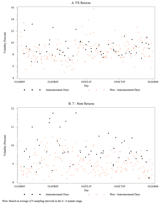
Figure 2. FX Realized Volatility Signature Plots for 3 Specific Dates
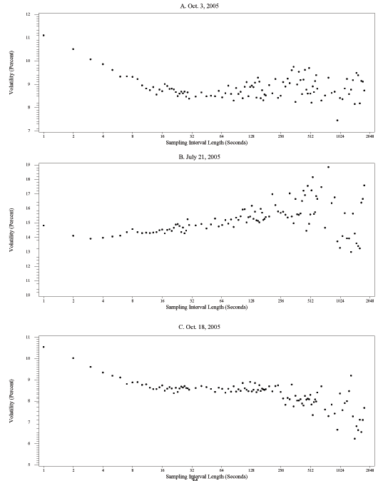
Figure 3. T-Note Realized Volatility Signature Plots for 3 Specific Dates
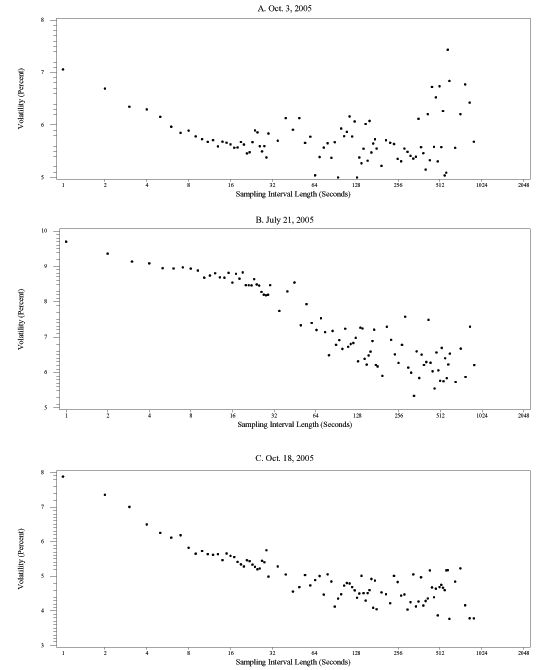
Figure 4. Realized Volatility Signature Plots and Announcement Effects
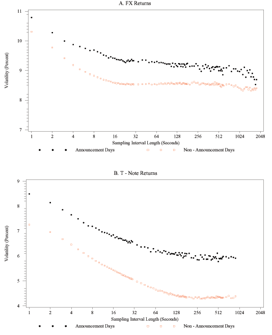
Figure 5. Dispersion of Estimates of Realized Volatility
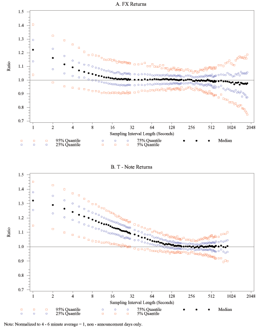
Figure 6. Optimal Sampling Frequencies Suggested by the Bandi-Russell Model
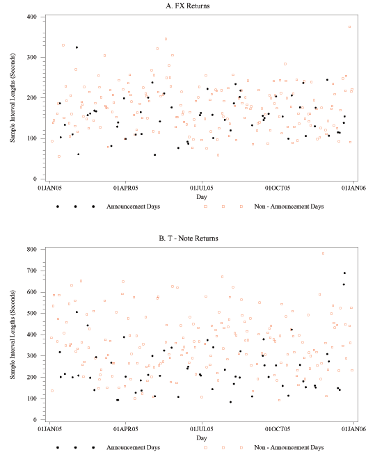
Figure 7. Autocorrelation Functions of Returns, Various Sampling Frequencies
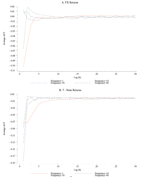
Figure 8. Optimal Choice of Bandwidth Parameter H, One-Second Returns
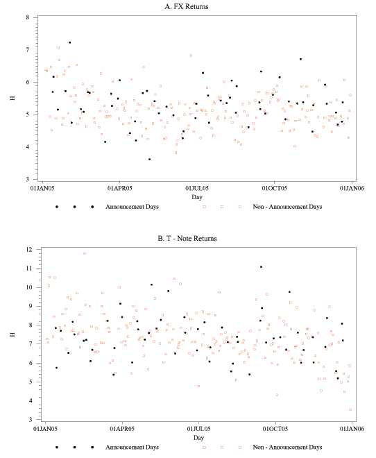
Figure 9. Kernel - Based Realized Volatility Signature Plots for FX Returns on 3 Specific Dates
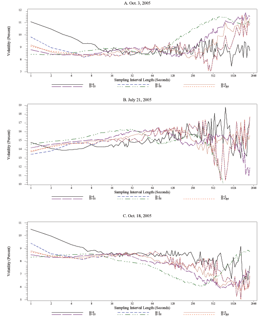
Figure 10. Kernel - Based Realized Volatility Signature Plots for T-Note Returns on 3 Specific Dates
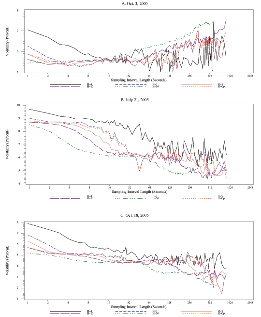
Figure 11. FX Time - Averaged Kernel - Based Realized Volatility Signature Plots
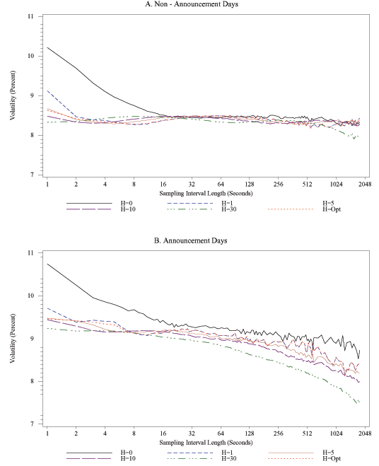
Figure 12. T-Note Time - Averaged Kernel - Based Realized Volatility Signature Plots
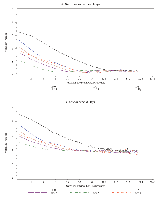
Figure 13. Realized Absolute Variation Signature Plots
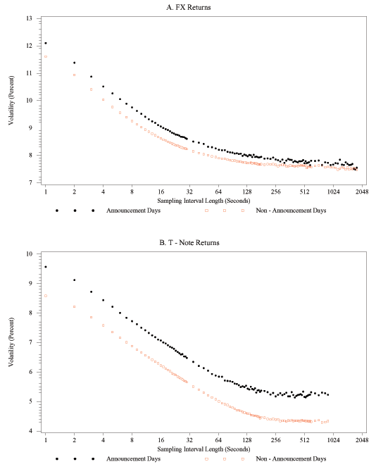
Figure 14. Realized Bipower Variation Signature Plots
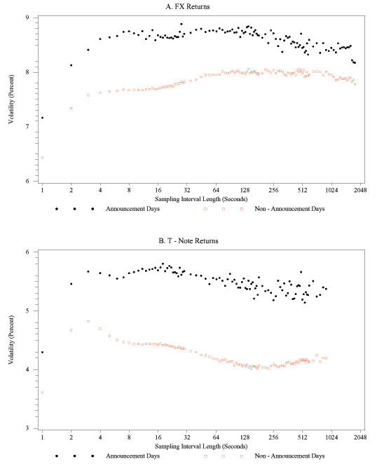
Figure 15. Realized Bipower Variation Signature Plots, Using Skip - One Returns
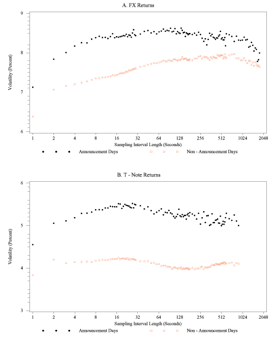
Footnotes
* Chaboud, Chiquoine, and Hjalmarsson are with the Division of International Finance, Federal Reserve Board, Washington DC 20551, USA. Loretan is with the Bank for International Settlements, Representative Office for Asia and the Pacific, 78/F Two International Finance Centre, 8 Finance Street, Central, Hong Kong SAR. Corresponding author: Erik Hjalmarsson; tel.: +1-202-452-2426; fax: +1-202-263-4850; email: [email protected]. The views in this paper are solely the responsibility of the authors and should not be interpreted as reflecting the views of the Board of Governors of the Federal Reserve System, of any other person associated with the Federal Reserve System, or of any other person associated with the Bank for International Settlements. Joshua Hausman provided excellent research assistance on an early version of this paper. We thank EBS (now part of ICAP) for the high-frequency foreign exchange data, and we are grateful to Jennifer Roush and Michael Fleming for providing access to the BrokerTec data. Celso Brunetti, Dobrislav Dobrev, Jacob Gyntelberg, Sam Ouliaris, Jun Yu, and seminar participants at Singapore Management University and National University of Singapore provided helpful comments and discussions. Any remaining errors are obviously our own. Return to text
1. In fact, Hansen and Lunde (2006) record as one of their empirical "facts" that market microstructure noise is negatively correlated with the returns, and hence biases the estimated volatility downward. However, as we show in this paper, this empirical stylized fact--which is based on their analysis of high-frequency stock returns--does not seem to carry over to the foreign exchange and bond markets. Return to text
2. The asymptotic properties of realized volatility and other related estimators have been primarily developed in a series of papers by Barndorff-Nielsen and Shephard (e.g., 2001, 2002ab, 2003, 2004ab, 2006). Other important contributions include, for instance, Andersen, Bollerslev, Diebold, and Labys (2001, 2003). A survey of this literature is given in Barndorff-Nielsen and Shephard (2005). Return to text
3. Aït-Sahalia et al. (2005)
study optimal sampling frequency rules that are similar to that
given by Bandi and Russell (2006b). Based on the market
microstructure model of Roll (1984), they suggest that the variance
of the market microstructure noise can be calculated from the
bid-ask spread in the data. In particular, if ![]() is the bid-ask spread in the market (expressed in percent of the
price), then
is the bid-ask spread in the market (expressed in percent of the
price), then
![]() . However, as
Aït-Sahalia et al. (2005) point out, by estimating
. However, as
Aït-Sahalia et al. (2005) point out, by estimating
![]() strictly from the bid-ask spread,
the contributions of any other sources to microstructure noise are
ignored. The resulting estimate of
strictly from the bid-ask spread,
the contributions of any other sources to microstructure noise are
ignored. The resulting estimate of
![]() should therefore be interpreted as
a lower bound on the actual variance of the noise. Return to text
should therefore be interpreted as
a lower bound on the actual variance of the noise. Return to text
4. Related studies include Andersen, Bollerslev, Diebold, and Ebens (2001) and Zhou (1996). Bandi and Russell (2006a) and Barndorff-Nielsen and Shephard (2005) provide surveys. Return to text
5. In our empirical work, we rely
exclusively on the Modified Tukey-Hanning kernel defined in BNHLS,
which additionally satisfies
![]() and is
asymptotically the most efficient of the kernels considered by
them. The Modified Tukey-Hanning kernel function is given by
and is
asymptotically the most efficient of the kernels considered by
them. The Modified Tukey-Hanning kernel function is given by
![]() ,
, ![]() . The bandwidth parameter
. The bandwidth parameter ![]() is set equal to
is set equal to
![]() , where
, where ![]() is a constant given in BNHLS. In the case when all
(or almost all) available data are used, i.e., when the data
sampled at or close to the highest available frequency, BNHLS
recommend using
is a constant given in BNHLS. In the case when all
(or almost all) available data are used, i.e., when the data
sampled at or close to the highest available frequency, BNHLS
recommend using
![]() ; we will rely on this
bandwidth choice for sampling intervals shorter than 30
seconds. Return to text
; we will rely on this
bandwidth choice for sampling intervals shorter than 30
seconds. Return to text
6. Equation (2) is thus a
special case of (14), with
![]() or, equivalently,
or, equivalently,
![]() for all
for all ![]() .
The assumption that
.
The assumption that ![]() is finite for
all
is finite for
all ![]() rules out certain processes, such as
stable-Lévy processes. Stable-Lévy processes are
characterized by an infinite number of jumps in any time interval.
See Calvet and Fisher (2002) for an overview of the theory and
empirical evidence of multifractal asset returns in finance;
multifractal processes are also characterized by an uncountable
number of jumps. Return to text
rules out certain processes, such as
stable-Lévy processes. Stable-Lévy processes are
characterized by an infinite number of jumps in any time interval.
See Calvet and Fisher (2002) for an overview of the theory and
empirical evidence of multifractal asset returns in finance;
multifractal processes are also characterized by an uncountable
number of jumps. Return to text
7. In the FX market, by global convention, the value date changes at 17:00 New York time (whether or not Daylight Saving time is in effect). This cutoff thus represents the threshold between two trading days. Return to text
8. The other leading electronic communication network (ECN) for trading in U.S. Treasuries is eSpeed. Return to text
9. Brokertec and EBS have both been acquired by ICAP in recent years. BrokerTec was acquired in 2003, EBS in 2006. Return to text
10. There are also several days in the sample for which the Bond Market Association recommended a 14:00 closing time. We account for these days in our calculations of realized volatilities by limiting the day to 08:00 to 14:00 New York time and scaling the estimated volatilities appropriately. Return to text
11. As a rule of thumb, in the present case a 1-percent change in the price of the bond corresponds to about a 13 basis point change in the yield. Return to text
12. Hence, the number of non-announcement days in the full sample is 184. Return to text
13. These realized volatilities are not
computed for a single sampling interval of, say, 5 minutes.
Instead, they are the averages of 9 separate volatility estimates,
obtained from returns for sample lengths of 4 minutes, 4'15",
4'30", ![]() , 5'45", and 6 minutes. We
elected to show these averaged realized volatility estimates
because, as we demonstrate in greater detail later, on any given
day these estimates can vary considerably even across
closely-spaced sampling frequencies. Return to text
, 5'45", and 6 minutes. We
elected to show these averaged realized volatility estimates
because, as we demonstrate in greater detail later, on any given
day these estimates can vary considerably even across
closely-spaced sampling frequencies. Return to text
14. On July 21, 2005, after close of business in China but before the start of the business day in North America, the Chinese authorities revalued their currency, the renminbi, by 2.1 percent against the U.S. dollar. On that day, foreign exchange market volatility was quite elevated in most major currency pairs. Return to text
15. We also observe that, in contrast to the case of non-announcement days, where the plot line is virtually flat for frequencies lower than the critical frequency, the plot line declines steadily (though only slightly) as the sampling interval length increases beyond 15 seconds. This suggests that FX trading dynamics on announcement days in 2005 may also have been characterized by a small amount of mean reversion at medium frequencies rather than just at the highest frequencies (as would be the case if the dynamics were purely of the microstructure variety). Return to text
16. For the bond returns, kernel estimates
with ![]() are not reported for the lowest
sampling frequencies, i.e. the longest sampling intervals, since
there are not enough observations available at these frequencies to
form an estimate when using
are not reported for the lowest
sampling frequencies, i.e. the longest sampling intervals, since
there are not enough observations available at these frequencies to
form an estimate when using ![]() lags. Return to text
lags. Return to text
17. For a Brownian diffusion,
![]() . For
dollar/euro returns from January 1999 to September 2006, the ratio
of the standard deviation of daily returns to the mean absolute
daily return was equal to 1.31, with yearly estimates of this
ratio falling in the interval
. For
dollar/euro returns from January 1999 to September 2006, the ratio
of the standard deviation of daily returns to the mean absolute
daily return was equal to 1.31, with yearly estimates of this
ratio falling in the interval
![]() . For 2005, this ratio
was 1.29, and it is this value, rather than
. For 2005, this ratio
was 1.29, and it is this value, rather than
![]() , that we use in the empirical
work on the volatility of FX returns in this section; for
daily-frequency returns on the 10-year Treasury note, the
corresponding ratio was 1.26 in 2005. The returns of many financial time series are generally much
more heavy-tailed than draws from a normal distribution are,
especially when the returns are sampled at very high frequencies.
For the case of the Student-
, that we use in the empirical
work on the volatility of FX returns in this section; for
daily-frequency returns on the 10-year Treasury note, the
corresponding ratio was 1.26 in 2005. The returns of many financial time series are generally much
more heavy-tailed than draws from a normal distribution are,
especially when the returns are sampled at very high frequencies.
For the case of the Student-![]() distribution (a
well-known class of heavy-tailed distributions), the ratio of the
distribution's standard deviation to its absolute first moment is a
function of
distribution (a
well-known class of heavy-tailed distributions), the ratio of the
distribution's standard deviation to its absolute first moment is a
function of ![]() , the degrees of freedom
parameter. For values of
, the degrees of freedom
parameter. For values of ![]() equal to 3,
5, and 10, this ratio is close to 1.57, 1.36,
and 1.29, respectively. In principle, this dependence of the
conversion factor on the distribution's tail shape parameter, and
the fact that the leptokurtosis of returns increases with the
sampling frequency, both indicate that that one should use a
conversion factor that varies systematically with the sampling
frequency. A full treatment of this issue is left to future
research. Return to text
equal to 3,
5, and 10, this ratio is close to 1.57, 1.36,
and 1.29, respectively. In principle, this dependence of the
conversion factor on the distribution's tail shape parameter, and
the fact that the leptokurtosis of returns increases with the
sampling frequency, both indicate that that one should use a
conversion factor that varies systematically with the sampling
frequency. A full treatment of this issue is left to future
research. Return to text
18. For a 24-hour (8-hour) trading day and a 1-second sampling frequency, the theoretical sample size is 86,400 (28,800). As is shown in Table 3, on an average trading day in 2005 the effective sample size for FX and bond returns at this frequency was only 13.9 percent and 7.6 percent, respectively, as large as the theoretical sample size. We note that these numbers represent averages across all trading days within the year. The fraction of 1-second intervals with non-zero returns within a day can vary considerably across days. Return to text
19. The volatility, rather than variance,
estimates are shown, i.e., results for
![]() are displayed. Return to text
are displayed. Return to text
20. This downward bias at higher sampling frequencies is especially prominent for FX returns. It is somewhat less pronounced for bond returns, except at the very highest sampling frequencies. Return to text
21. Note that in the case of the absolute power variation method, a natural way for adjusting the estimator for changes in the prevalence of intervals with zero returns is to adjust the sample size, i.e., to set the sample size equal to the number of intervals with non-zero returns. No such simple adjustment is available for the estimator that is based on the bipower variation of returns. We conjecture that, when computing the bipower variation of a discretely-generated process, a practical method for dealing with the incidence of intervals with zero returns is to discard all samples that have zero returns prior to calculating the bipower products. Return to text
22. It is also possible that the workup process on BrokerTec affects bond price dynamics in a way that makes market microstructure noise persist longer than in FX markets. BrokerTec has recently changed the mechanics of its workup process significantly. Return to text
This version is optimized for use by screen readers. Descriptions for all mathematical expressions are provided in LaTex format. A printable pdf version is available. Return to text