
Board of Governors of the Federal Reserve System
International Finance Discussion Papers
Number 915, December 2007 --- Screen Reader
Version*
Testing for Cointegration Using the Johansen Methodology when Variables are Near-Integrated *
NOTE: International Finance Discussion Papers are preliminary materials circulated to stimulate discussion and critical comment. References in publications to International Finance Discussion Papers (other than an acknowledgment that the writer has had access to unpublished material) should be cleared with the author or authors. Recent IFDPs are available on the Web at http://www.federalreserve.gov/pubs/ifdp/. This paper can be downloaded without charge from the Social Science Research Network electronic library at http://www.ssrn.com/.
Abstract:
We investigate the properties of Johansen's (1988, 1991) maximum eigenvalue and trace tests for cointegration under the empirically relevant situation of near-integrated variables. Using Monte Carlo techniques, we show that in a system with near-integrated variables, the probability of reaching an erroneous conclusion regarding the cointegrating rank of the system is generally substantially higher than the nominal size. The risk of concluding that completely unrelated series are cointegrated is therefore non-negligible. The spurious rejection rate can be reduced by performing additional tests of restrictions on the cointegrating vector(s), although it is still substantially larger than the nominal size.
Keywords: Cointegration, near-unit-roots, spurious rejection, Monte Carlo simulations
JEL classification: C12, C15, C32
1 Introduction
Cointegration methods have been very popular tools in applied economic work since their introduction about twenty years ago. However, the strict unit-root assumption that these methods typically rely upon is often not easy to justify on economic or theoretical grounds. For instance, variables such as inflation, interest rates, real exchange rates and unemployment rates all appear to be highly persistent, and are frequently modelled as unit root processes. But, there is little a priori reason to believe that these variables have an exact unit root, rather than a root close to unity. In fact, these variables often show signs of mean reversion in long enough samples.1 Since unit-root tests have very limited power to distinguish between a unit-root and a close alternative, the pure unit-root assumption is typically based on convenience rather than on strong theoretical or empirical facts. This has led many economists and econometricians to believe near-integrated processes, which explicitly allow for a small (unknown) deviation from the pure unit-root assumption, to be a more appropriate way to describe many economic time series; see, for example, Stock (1991), Cavanagh et al., (1995) and Elliott (1998).2
Near-integrated and integrated time series have implications for estimation and inference that are similar in many respects. For instance, spurious regressions are a problem when variables are near-integrated as well as integrated, and therefore, it is also relevant to discuss cointegration of near-integrated variables; see Phillips (1988) for an analytical discussion regarding these issues. Unfortunately, inferential procedures designed for data generated by unit-root processes tend not to be robust to deviations from the unit-root assumption. For instance, Elliott (1998) shows that large size distortions can occur when performing inference on the cointegration vector in a system where the individual variables follow near-unit-root processes rather than pure unit-root processes.
The purpose of this paper is to investigate the effect of deviations from the unit-root assumption on the determination of the cointegrating rank of the system using Johansen's (1988, 1991) maximum eigenvalue and trace tests. Unlike inference regarding the cointegrating vectors, this issue has not been investigated much in the literature. The first contribution of the current paper is therefore to document the rejection rates for standard tests of cointegration, using the Johansen framework, in a system where the variables are near-integrated. Through extensive Monte Carlo simulations, we show that the probability of reaching an erroneous conclusion regarding the cointegrating rank of the system is generally substantially higher than the nominal size. That is, the nominal size of the test can vastly understate the risks of finding a spurious relationship between unrelated near-integrated variables. In a simple bivariate system, the spurious rejection rate can approach 20 and 40 percent for the maximum eigenvalue and trace tests respectively, using a nominal size of five percent. Even higher rejection rates are found in a trivariate system. The second contribution is to show how a sequence of additional tests on the cointegrating vector(s) can help improve the performance of the tests and reduce the spurious rejection rate. However, even after taking these extra steps, the rejection rate of the test is still considerably larger than the nominal size. This is particularly true for the trivariate system where spurious rejection rates between 15 and 20 percent are documented for nominal five percent tests.
Overall, the performance of the trace test appears worse than that of the maximum eigenvalue test. Both tests, however, have large enough deviations from the nominal size that practitioners should be aware of the problems associated with Johansen's procedures under these circumstances. The proposed sequence of additional tests helps alleviate some of the sensitivity of the Johansen procedures to deviations from the strict unit-root assumption. They do not, however, eliminate the problem.
The remainder of this paper is organised as follows: Section 2 gives a brief introduction to Johansen's methodology and Section 3 presents the Monte Carlo study. In Section 4, we present an empirical illustration of the problems associated with near-integrated variables using U.S. data on CPI inflation and the short nominal interest rate. Section 5 concludes.
2 Testing for Cointegration Using Johansen's Methodology
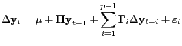
Johansen's methodology takes its starting point in the vector
autoregression (VAR) of order ![]() given by
given by
| (1) |
where
![]() is an
is an ![]() x1
vector of variables that are integrated of order one - commonly
denoted I(1) - and
x1
vector of variables that are integrated of order one - commonly
denoted I(1) - and
![]() is an
is an
![]() x1 vector of innovations. This VAR can be
re-written as
x1 vector of innovations. This VAR can be
re-written as
|
(2) |
where
 and
and
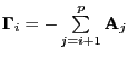 . . |
(3) |
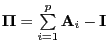
If the coefficient matrix
![]() has reduced rank
has reduced rank
![]() , then there exist
, then there exist ![]() x
x![]() matrices
matrices
![]() and
and
![]() each with rank
each with rank
![]() such that
such that
![]() and
and
![]() is
stationary.
is
stationary. ![]() is the number of cointegrating
relationships, the elements of
is the number of cointegrating
relationships, the elements of
![]() are known as the
adjustment parameters in the vector error correction model and each
column of
are known as the
adjustment parameters in the vector error correction model and each
column of
![]() is a cointegrating
vector. It can be shown that for a given
is a cointegrating
vector. It can be shown that for a given ![]() , the
maximum likelihood estimator of
, the
maximum likelihood estimator of
![]() defines the
combination of
defines the
combination of
![]() that yields the
that yields the
![]() largest canonical correlations of
largest canonical correlations of
![]() with
with
![]() after correcting
for lagged differences and deterministic variables when
present.3 Johansen proposes two different
likelihood ratio tests of the significance of these canonical
correlations and thereby the reduced rank of the
after correcting
for lagged differences and deterministic variables when
present.3 Johansen proposes two different
likelihood ratio tests of the significance of these canonical
correlations and thereby the reduced rank of the
![]() matrix: the trace test
and maximum eigenvalue test, shown in equations (4) and (5)
respectively.
matrix: the trace test
and maximum eigenvalue test, shown in equations (4) and (5)
respectively.
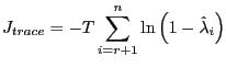
|
(3) |
| (4) |
Here ![]() is the sample size and
is the sample size and
![]() is the
is the ![]() :th largest canonical correlation. The trace test tests the
null hypothesis of
:th largest canonical correlation. The trace test tests the
null hypothesis of ![]() cointegrating vectors
against the alternative hypothesis of
cointegrating vectors
against the alternative hypothesis of ![]() cointegrating
vectors. The maximum eigenvalue test, on the other hand, tests the
null hypothesis of
cointegrating
vectors. The maximum eigenvalue test, on the other hand, tests the
null hypothesis of ![]() cointegrating vectors
against the alternative hypothesis of
cointegrating vectors
against the alternative hypothesis of ![]() cointegrating vectors. Neither of these test statistics follows a
chi square distribution in general; asymptotic critical values can
be found in Johansen and Juselius (1990) and are also given by most
econometric software packages. Since the critical values used for
the maximum eigenvalue and trace test statistics are based on a
pure unit-root assumption, they will no longer be correct when the
variables in the system are near-unit-root processes.4 Thus,
the real question is how sensitive Johansen's procedures are
to deviations from the pure-unit root assumption.
cointegrating vectors. Neither of these test statistics follows a
chi square distribution in general; asymptotic critical values can
be found in Johansen and Juselius (1990) and are also given by most
econometric software packages. Since the critical values used for
the maximum eigenvalue and trace test statistics are based on a
pure unit-root assumption, they will no longer be correct when the
variables in the system are near-unit-root processes.4 Thus,
the real question is how sensitive Johansen's procedures are
to deviations from the pure-unit root assumption.
Although Johansen's methodology is typically used in a setting
where all variables in the system are I(1), having
stationary variables in the system is theoretically not an issue
and Johansen (1995) states that there is little need to pre-test
the variables in the system to establish their order of
integration. If a single variable is I(0) instead of I(1), this will
reveal itself through a cointegrating vector whose space is spanned
by the only stationary variable in the model. For instance, if the
system in equation (2)
describes a model in which
![]() where
where ![]() is I(1) and
is I(1) and ![]() is I(0), one should expect to find that there is one
cointegrating vector in the system which is given by
is I(0), one should expect to find that there is one
cointegrating vector in the system which is given by
![]() . In the case where
. In the case where
![]() has full rank, all
has full rank, all
![]() variables in the system are
stationary.5
variables in the system are
stationary.5
The fact that stationary variables in a system will introduce restricted cointegrating vectors is something that should be kept in mind in empirical work. That is, it is good econometric practice to always include tests on the cointegrating vectors to establish whether relevant restrictions are rejected or not. If such restrictions are not tested, a non-zero cointegrating rank might mistakenly be taken as evidence in favour of cointegration between variables. This is particularly relevant when there are strong prior opinions regarding which variables "have to" be in the cointegrating relationship. An obvious example is the literature on equilibrium real exchange rates. For example, in studies using the so-called BEER approach - which relates the real exchange rate to its fundamental determinants - cointegration techniques are extremely common.6 After finding support for a cointegrating vector in a system, it is almost always the case in that literature that the coefficient on the real exchange rate is normalized to one, thereby forcing it to be part of the cointegrating relationship. However, tests of whether all other coefficients in the cointegrating vector are zero are rarely performed. Even rarer are tests of whether the only cointegrating vector is due to the stationarity of some other variable in the system, despite the fact that the proposed determinants of real exchange rates in many cases can be argued to be stationary.
The lack of need to a priori distinguish between
I(1) and I(0)
variables is based on the assumption that any variable that is not
I(1), or a pure
unit-root process, is a stationary I(0) process. This apparent
flexibility, therefore, does not make the method robust to
near-integrated variables, since they fall into neither of these
two classifications. However, the above specification tests of the
cointegrating vector suggest a way of making inference more robust
in the potential presence of near-unit-root variables. For
instance, considering the bivariate case described above,
explicitly testing whether
![]() will help to rule out spurious relationships that are not rejected
by the initial maximum eigenvalue or trace test.7 Although we argue
that such specification tests should be performed in almost every
kind of application, they are likely to be extra useful in cases
where the variables are likely to have near-unit-roots and the
initial test of cointegration rank is biased.8
will help to rule out spurious relationships that are not rejected
by the initial maximum eigenvalue or trace test.7 Although we argue
that such specification tests should be performed in almost every
kind of application, they are likely to be extra useful in cases
where the variables are likely to have near-unit-roots and the
initial test of cointegration rank is biased.8
3 Monte Carlo Study
3.1 Setup
The data generating process (DGP) for the ![]() x1
vector
x1
vector
![]() is given by
is given by
| (5) |
where ![]() is the local-to-unity parameter that, for
simplicity, is assumed to be common to all variables,
is the local-to-unity parameter that, for
simplicity, is assumed to be common to all variables,
![]() is the
is the ![]() x
x![]() identity matrix, and
identity matrix, and
![]() is an
is an
![]() x1 vector of normally distributed iid
disturbances such that
x1 vector of normally distributed iid
disturbances such that
![]() and
and
![]() . We investigate the spurious rejection frequency of the Johansen
maximum eigenvalue and trace tests for systems of size
. We investigate the spurious rejection frequency of the Johansen
maximum eigenvalue and trace tests for systems of size
![]() and set the sample size to
and set the sample size to
![]() , which covers most empirically relevant cases. For all
combinations of
, which covers most empirically relevant cases. For all
combinations of ![]() and
and ![]() , we let
, we let
![]() take on values between 0 and -60.9 The
nominal size of all tests is set to five percent.
take on values between 0 and -60.9 The
nominal size of all tests is set to five percent.
We estimate the VAR in equation (2). Given the DGP
in equation (6), lag
length in the VAR is set to the correct value of ![]() . Furthermore, we use the empirically most common
specification, which allows for a constant in the cointegrating
relationship but no deterministic trend in the data. For notational
convenience, the constant term will be suppressed in the following
analysis.
. Furthermore, we use the empirically most common
specification, which allows for a constant in the cointegrating
relationship but no deterministic trend in the data. For notational
convenience, the constant term will be suppressed in the following
analysis.
Since the variables in the system are completely unrelated, the
frequency with which evidence of a cointegrating relationship is
found should ideally be equal to the nominal size.10
However, rejection of the null hypothesis,
![]() , does not automatically lead to
the false conclusion that there is cointegration between the
variables in the system. In the bivariate case, rejecting
, does not automatically lead to
the false conclusion that there is cointegration between the
variables in the system. In the bivariate case, rejecting
![]() will not lead to a rejection of
the null hypothesis of no cointegration if:
will not lead to a rejection of
the null hypothesis of no cointegration if:
a) H0 : r = 1 is also rejected. For the DGP
considered above, this implies that both variables are stationary
as the matrix
![]() has full rank.
has full rank.
b) H0 : r = 1 cannot be rejected but the
restriction
![]() or ii)
or ii)
![]() cannot be rejected either. In either of these cases, we would
conclude that there is no cointegration between
cannot be rejected either. In either of these cases, we would
conclude that there is no cointegration between ![]() and
and ![]() . If the restriction in
. If the restriction in
![]() is judged valid, the conclusion is that
is judged valid, the conclusion is that
![]() is stationary and that it does not
have a long-run relationship with
is stationary and that it does not
have a long-run relationship with ![]() . If the
restriction in ii) is instead judged valid, the conclusion
drawn would be symmetric.
. If the
restriction in ii) is instead judged valid, the conclusion
drawn would be symmetric.
In the trivariate case, rejecting
![]() will not lead to a rejection of
the null hypothesis of no cointegration if:
will not lead to a rejection of
the null hypothesis of no cointegration if:
c) H0 : r = 1 and H0 : r = 2 are also rejected. For the DGP
considered above, this implies that all three variables are
stationary as the matrix
![]() has full rank.
has full rank.
d) H0 : r = 1 cannot be rejected but the
restriction iii)
![]() , iv)
, iv)
![]() or
or
![]() also cannot be rejected. Similar to the bivariate case
also cannot be rejected. Similar to the bivariate case ![]() , we would conclude that the only cointegrating vector in
the system is due to a stationary variable rather than
cointegration between variables.
, we would conclude that the only cointegrating vector in
the system is due to a stationary variable rather than
cointegration between variables.
e) H0 : r = 1 is rejected but H0 : r = 2 is not, at the same time as the
restrictions vi)
 , vii)
 or viii)
 cannot be rejected. Just like in
 ![]() and
and
![]() , we would conclude that there is no
cointegration between variables and that the cointegrating vectors
are due to stationary variables.
, we would conclude that there is no
cointegration between variables and that the cointegrating vectors
are due to stationary variables.
The interpretation of the restrictions on the cointegrating
vector offered above - that variables may be integrated of
different orders - is clearly not strictly correct since we know
that all variables are near-integrated with the same local-to-unity
parameter. However, it is the interpretation that an applied
researcher, working within the implicit assumptions of the Johansen
framework, would draw. Finally, it should be pointed out that the
above testing scheme raises some concerns regarding the properties
of the tests under the alternative of cointegration. In particular,
when the matrix
![]() is found to have full
rank - and all
is found to have full
rank - and all ![]() variables in the system accordingly
are judged stationary - the abilitiy to actually detect
cointegration among stationary near-integrated variables is
limited. Although outside the scope of this paper, such issues
clearly need to be addressed in a formal extension of the Johansen
framework to near-integrated variables.
variables in the system accordingly
are judged stationary - the abilitiy to actually detect
cointegration among stationary near-integrated variables is
limited. Although outside the scope of this paper, such issues
clearly need to be addressed in a formal extension of the Johansen
framework to near-integrated variables.
3.2 Results
Figures 1 and 2 show the spurious rejection frequencies for the
bivariate and trivariate systems respectively. The left columns in
both figures show the spurious rejection frequencies when the
cointegrating rank of the system alone is taken as evidence of
cointegration between variables. This is simply when we conclude
that ![]() in the bivariate case and either
in the bivariate case and either
![]() or
or ![]() in the
trivariate case. Recall that
in the
trivariate case. Recall that ![]() or
or ![]() both imply that a correct conclusion has been drawn since
the variables in the systems here are completely unrelated. In the
right column, on the other hand, the additional tests in
both imply that a correct conclusion has been drawn since
the variables in the systems here are completely unrelated. In the
right column, on the other hand, the additional tests in
![]() ,
, ![]() or
or ![]() are also conducted. This means that the correct conclusion
of no cointegration between variables can be drawn also for
are also conducted. This means that the correct conclusion
of no cointegration between variables can be drawn also for
![]() in the bivariate case and for
in the bivariate case and for
![]() or
or ![]() in the
trivariate case and not only for
in the
trivariate case and not only for ![]() or
or ![]() .
.
Figure 1. Spurious rejection frequency for bivariate system.
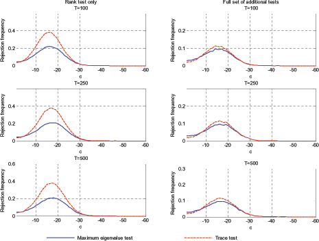
Figure 2. Spurious rejection frequency for trivariate system.
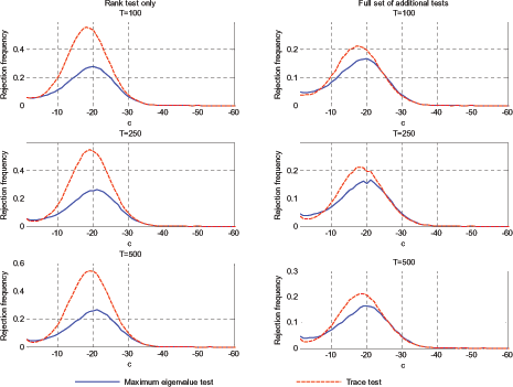
Conisdering the bivariate system in Figure 1, it is clear from
the left column that if one relies exclusively on the estimated
rank of the system for inference, there is a large risk of
spuriously concluding that completely unrelated variables are
cointegrated. When ![]() is small in absolute value,
the rejection frequency is close to the nominal size. However, it
is evident already for
is small in absolute value,
the rejection frequency is close to the nominal size. However, it
is evident already for ![]() that the tests are
severely over rejecting; in particular, the trace test has very
poor properties with a spurious rejection frequency of
approximately 18 percent. The problem reaches a peak for a value of
that the tests are
severely over rejecting; in particular, the trace test has very
poor properties with a spurious rejection frequency of
approximately 18 percent. The problem reaches a peak for a value of
![]() , where the maximum eigenvalue and
trace tests reach spurious rejection frequencies of approximately
21 and 38 percent respectively, regardless of sample size. As
, where the maximum eigenvalue and
trace tests reach spurious rejection frequencies of approximately
21 and 38 percent respectively, regardless of sample size. As
![]() becomes even larger in absolute value, the
rejection frequency falls and approaches zero for
becomes even larger in absolute value, the
rejection frequency falls and approaches zero for ![]() . The reason for this is that both the maximum
eigenvalue and trace test correctly conclude that
. The reason for this is that both the maximum
eigenvalue and trace test correctly conclude that ![]() ; that is, that both variables are stationary. The top row
of Figure A1 in the Appendix further illustrates this phenomenon by
showing the results for the individual rank tests in the case of
; that is, that both variables are stationary. The top row
of Figure A1 in the Appendix further illustrates this phenomenon by
showing the results for the individual rank tests in the case of
![]() . Turning to the right column in Figure
1, it can be seen that if tests of
. Turning to the right column in Figure
1, it can be seen that if tests of
![]() and
and
![]() are conducted, after failing to reject that
are conducted, after failing to reject that ![]() , the spurious rejection frequency falls dramatically for
both tests. However, while the problem is alleviated, it is still
concluded that there is a cointegrating relationship around ten
percent of the time when
, the spurious rejection frequency falls dramatically for
both tests. However, while the problem is alleviated, it is still
concluded that there is a cointegrating relationship around ten
percent of the time when ![]() is in the neighbourhood of
-17; this is the case regardless of the test used.
is in the neighbourhood of
-17; this is the case regardless of the test used.
The results for the trivariate system shown in Figure 2 are
qualitatively very similar to those from the bivariate system, but
the problem of spurious rejection is quantitatively worse for the
larger system. There is a large interval of values for ![]() , for which both the maximum eigenvalue and trace tests have
very high spurious rejection frequencies, regardless of whether we
look solely at the rank (left column) or conduct the additional
tests after determining the rank (right column). For a
, for which both the maximum eigenvalue and trace tests have
very high spurious rejection frequencies, regardless of whether we
look solely at the rank (left column) or conduct the additional
tests after determining the rank (right column). For a ![]() of approximately -18 to -20, the rejection frequency is at
its highest. Even if the additional tests on the cointegrating
vectors are conducted, the maximum eigenvalue and trace tests have
unacceptably high rejection rates: 16 and 21 percent respectively
regardless of sample size. Finally, for
of approximately -18 to -20, the rejection frequency is at
its highest. Even if the additional tests on the cointegrating
vectors are conducted, the maximum eigenvalue and trace tests have
unacceptably high rejection rates: 16 and 21 percent respectively
regardless of sample size. Finally, for ![]() or
smaller, the spurious rejection frequency is virtually zero as both
tests always conclude that the rank of
or
smaller, the spurious rejection frequency is virtually zero as both
tests always conclude that the rank of
![]() is equal to three.
This is again further illustrated in the bottom row of Figure A1 in
the Appendix.
is equal to three.
This is again further illustrated in the bottom row of Figure A1 in
the Appendix.
Summing up, neither the maximum eigenvalue nor the trace test is
reliable in terms of assessing whether variables are cointegrated
when the data do not have exact unit roots. For reasonable values
of ![]() , the spurious rejection frequency can be
several times higher than the nominal size.
, the spurious rejection frequency can be
several times higher than the nominal size.
4 An Empirical Illustration
We next turn to an empirical application where it can be argued that the DGP underlying the series is potentially near-integrated. Given the high persistence of nominal interest rates and inflation in many countries, a popular approach to test the Fisher hypothesis in more recent years has been to employ cointegration techniques; see, for example, MacDonald and Murphy (1989), Wallace and Warner (1993), Crowder and Hoffman (1996) and Junttila (2001). This makes sense to some extent as it has been pointed out that the Fisher hypothesis is better interpreted as a long-run equilibrium condition (Summers, 1983). However, much research has questioned the implicit or explicit assumption in these papers that inflation and the nominal interest rate are I(1); see, for example, Wu and Zhang (1996), Culver and Papell (1997), Lee and Wu (2001), Wu and Chen (2001) and Basher and Westerlund (2006). The existence of exact unit-roots in either inflation or nominal interest rates is thus far from certain, and it is interesting to revisit the question of cointegration between them in the light of the above Monte Carlo study.
Figure 3. Data
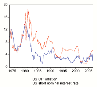
We use monthly data on the US short nominal interest rate, given
by the three month treasury bill and denoted ![]() , and CPI inflation,
, and CPI inflation, ![]() , from
January 1974 to October 2006. Data were provided by the Board of
Governors of the Federal Reserve System and are shown in Figure
3.
, from
January 1974 to October 2006. Data were provided by the Board of
Governors of the Federal Reserve System and are shown in Figure
3.
Table 1 shows the results from the Augmented Dickey-Fuller (Said
and Dickey, 1984) unit root test, where lag length has been
established using the Akaike (1974) information criterion. As can
be seen, the null hypothesis of a unit root cannot be rejected for
either variable. In addition, Table 1 shows the 95% confidence
intervals for the local-to-unity parameter ![]() and the
corresponding autoregressive root
and the
corresponding autoregressive root ![]() =1
=1![]() , for each of the variables.
These are obtained by inverting the ADF test statistic as described
in Stock (1991). The range of possible values for
, for each of the variables.
These are obtained by inverting the ADF test statistic as described
in Stock (1991). The range of possible values for ![]() clearly covers the values for which the largest spurious rejection
rates were recorded in the Monte Carlo study.
clearly covers the values for which the largest spurious rejection
rates were recorded in the Monte Carlo study.
Table 1. Results from Augmented Dickey-Fuller test.
Variable | τADF | 95% confidence interval for c | 95% confidence interval for ρ |
|---|---|---|---|
| πt | -2.271 (0.182) | [-18.019, 2.776] | [0.954, 1.007] |
| it | -2.722 (0.071) | [-24.144, 1.680] | [0.939, 1.004] |
Note: p-value in parentheses ().
Next, we turn to the issue of determining the cointegrating rank
of the system, which is done by estimating equation (2) with
![]() . Lag length is set to
. Lag length is set to ![]() based on the Akaike
information criterion and the constant is restricted to allow for
an intercept in the cointegrating relationship but no deterministic
trend in the data. Table 2 shows the results from the cointegration
tests. Both tests reject the null of zero cointegrating vectors.
The hypothesis that there is one cointegrating vector cannot be
rejected on the other hand; that is, based on the cointegration
test, there is no support for both variables in the system being
stationary. Based solely on the evidence in Table 2, we would
conclude that there exists a cointegrating relationship.
based on the Akaike
information criterion and the constant is restricted to allow for
an intercept in the cointegrating relationship but no deterministic
trend in the data. Table 2 shows the results from the cointegration
tests. Both tests reject the null of zero cointegrating vectors.
The hypothesis that there is one cointegrating vector cannot be
rejected on the other hand; that is, based on the cointegration
test, there is no support for both variables in the system being
stationary. Based solely on the evidence in Table 2, we would
conclude that there exists a cointegrating relationship.
Table 2. Results from cointegration test.
Null hypothesis | Jtrace | Jmax |
|---|---|---|
| r = 0 | 22.045 (0.028) | 16.402 (0.042) |
| r = 1 | 5.642 (0.220) | 5.642 (0.220) |
Note: p-value in parentheses ().
Typically, finding that the rank of
![]() is one in the system
above is taken as evidence for cointegration between the nominal
interest rate and inflation. Following good econometric practice,
we should, however, also test whether the cointegrating vector
satisfies either the restriction
is one in the system
above is taken as evidence for cointegration between the nominal
interest rate and inflation. Following good econometric practice,
we should, however, also test whether the cointegrating vector
satisfies either the restriction
![]() or
or
![]() . As shown in the Monte Carlo study above, these additional tests
also substantially reduce the risk of spuriously concluding that
near-integrated variables are cointegrated. The results are given
in Table 3 and, as can be seen,
. As shown in the Monte Carlo study above, these additional tests
also substantially reduce the risk of spuriously concluding that
near-integrated variables are cointegrated. The results are given
in Table 3 and, as can be seen,
![]() is rejected whereas the restriction
is rejected whereas the restriction
![]() is not. Our conclusion is hence that the above finding of a
cointegrating vector does not lend support for cointegration
between the nominal interest rate and inflation. Instead, based on
conducted tests, the empirical evidence points to the nominal
interest rate and inflation being integrated of different orders.
In such a case, no long-run equilibrium relationship can exist
between the two.11
is not. Our conclusion is hence that the above finding of a
cointegrating vector does not lend support for cointegration
between the nominal interest rate and inflation. Instead, based on
conducted tests, the empirical evidence points to the nominal
interest rate and inflation being integrated of different orders.
In such a case, no long-run equilibrium relationship can exist
between the two.11
Table 3. Results from hypothesis tests on the cointegrating vector.
Restriction | Test statistic |
|---|---|
| | 6.911 (0.009) |
| | 0.391 (0.532) |
Note: p-value in parentheses ().
5 Conclusion
This paper has investigated the properties of Johansen's maximum eigenvalue and trace tests for cointegration under the empirically relevant situation of near-integrated variables. Overall, the results show that there is a substantial probability, much larger than the nominal size of the test, of falsely concluding that completely unrelated series are cointegrated. We find that a systematic check of additional tests on the cointegrating vector(s) - based on Johansen's claim that there is little need to pre-test variables for unit roots - helps reduce the spurious rejection frequency. However, the spurious rejection frequency remains large and appears to increase with the number of variables in the system, even after applying such specification tests.
The results are obtained in a Monte Carlo simulation under perfect circumstances. That is, the data are normally distributed and the lag-length in the VAR in levels is known and equal to one. In practice, we do not have the benefit of being given the correct model - neither in terms of the variables in the system nor the lag length - and the problems shown in this paper are likely to be exacerbated.
The findings in this paper further illustrate the sensitivity of cointegration methods to deviations from the pure unit-root assumption, as originally noted by Elliott (1998) in regards to inference on the cointegrating vectors. Since unit-root tests cannot easily distinguish between a unit root and close alternatives, this raises a precautionary note to the interpretation of results from cointegration studies. In particular, it raises questions regarding the conclusions drawn in previous studies that have relied on cointegrating methods despite having found evidence of stationarity of the included variables; see, for example, Crowder and Hoffman (1996) and Granville and Mallick (2004). One way of making the Johansen procedure more robust to near-unit-roots may be through a Bonferroni type bounds procedure as proposed by Cavanagh et al. (1995) for inference on the cointegrating vector and by Hjalmarsson and Österholm (2007) for residual-based tests of cointegration.
References
Akaike, H. (1974), "A New Look at the Statistical Model Identification", IEEE Transactions on Automatic Control 19, 716-723.
Bagchi, D., Chortareas, G. E. and Miller, S. M. (2004), "The Real Exchange Rate in Small, Open, Developed Economies: Evidence from Cointegration Analysis", Economic Record 80, 76-88.
Basher, S. and Westerlund, J. (2006), "Is there Really a Unit Root in the Inflation Rate? More Evidence from Panel Data Models", Forthcoming in Applied Economics Letters.
Campbell, J.Y., and Yogo M. (2006), "Efficient Tests of Stock Return Predictability", Journal of Financial Economics 81, 27-60.
Cardoso, E. (1998), "Virtual Deficits and the Patinkin Effect", IMF Staff Papers 45, 619-646.
Cavanagh, C., Elliot, G., and Stock J. (1995). "Inference in Models with Nearly Integrated Regressors", Econometric Theory 11, 1131-1147.
Clark, P. B. and MacDonald, R. (1999), "Exchange Rates and Economic Fundamentals: A Methodological Comparison of BEERs and FEERs", In: MacDonald, R. and Stein, J. L. (eds) Equilibrium Exchange Rates. Kluwer Academic Press, Norwell.
Crowder, W. J. and Hoffman, D. L. (1996), "The Long-Run Relationship between Nominal Interest Rates and Inflation: The Fisher Equation Revisited", Journal of Money, Credit and Banking 28, 102-118.
Culver, S. E. and Papell, D. H. (1997), "Is there a Unit Root in the Inflation Rate? Evidence from Sequential Break and Panel Data Models", Journal of Applied Econometrics 12, 436-444.
Elliott, G. (1998), "On the Robustness of Cointegration Methods When Regressors Almost Have Unit Roots", Econometrica 66, 149-158.
Granville, B. and Mallick, S. (2004), "Fisher Hypothesis: UK Evidence over a Century", Applied Economics Letters 11, 87-90.
Hjalmarsson, E. and Österholm, P. (2007), "Residual-Based Tests of Cointegration for Near-Unit-Root Variables", International Finance Discussion Papers 907, Board of Governors of the Federal Reserve System.
Johansen, S. (1988), "Statistical Analysis of Cointegration Vectors", Journal of Economic Dynamics and Control 12, 231-254.
Johansen, S. (1991), "Estimation and Hypothesis Testing of Cointegration Vectors in Gaussian Vector Autoregressive Models", Econometrica 59, 1551-1580.
Johansen, S. (1995), Likelihood-Based Inference in Cointegrated Vector Autoregressive Models. Oxford University Press, New York.
Johansen, S. and Juselius, K. (1990), "Maximum Likelihood Estimation and Inference on Cointegration - with Applications to the Demand for Money", Oxford Bulletin of Economics and Statistics 52, 169-210.
Jonsson, G. (2001), "Inflation, Money Demand, and Purchasing Power Parity in South Africa", IMF Staff Papers 48, 243-265.
Junttila, J. (2001), "Testing an Augmented Fisher Hypothesis for a Small Open Economy: The Case of Finland", Journal of Macroeconomics 23, 577-599.
Khamis, M. and Leone, A. M. (2001), "Can Currency Demand Be Stable under a Financial Crisis? The Case of Mexico", IMF Staff Papers 48, 344-366.
Lee, H.-Y. and Wu, J.-L. (2001), "Mean Reversion of Inflation Rates: Evidence from 13 OECD Countries", Journal of Macroeconomics 23, 477-487.
MacDonald, R. and Murphy, P. D. (1989), "Testing the Long Run Relationship between Nominal Interest Rates and Inflation Using Cointegration Techniques", Applied Economics 21, 439-447.
Malley, J. and Moutos, T. (1996), "Unemployment and Consumption", Oxford Economic Papers 48, 584-600.
Österholm, P. (2004), "Killing Four Unit Root Birds in the US Economy with Three Panel Unit Root Test Stones", Applied Economics Letters 11, 213-216.
Phillips, P. C. B. (1988), "Regression Theory for Near-Integrated Time Series", Econometrica 56, 1021-1043.
Rose, A. K. (1988), "Is the Real Interest Rate Stable?", Journal of Finance 43, 1095-1112.
Song, F. M. and Wu, Y. (1997), "Hysteresis in Unemployment: Evidence from 48 US States", Economic Inquiry 35, 235-243.
Song, F. M. and Wu, Y. (1998), "Hysteresis in Unemployment: Evidence from OECD Countries", Quarterly Review of Economics and Finance 38,181-192.
Stock, J.H. (1991), "Confidence Intervals for the Largest Autoregressive Root in U.S. Economic Time-Series", Journal of Monetary Economics 28, 435-460.
Summers, L. H. (1983), "The Nonadjustment of Nominal Interest Rates: A Study of the Fisher Effect", In: Tobin, J. (ed) Macroeconomics, Prices and Quantities: Essays in Memory of Arthur M. Okun. Blackwell, Oxford.
Taylor, M. P. and Sarno, L. (1998), "The Behaviour of Real
Exchange Rates During
the Post-Bretton Woods Period", Journal of International
Economics 46, 281-312.
Wallace, M. and Warner, J. (1993), "The Fisher Effect and the Term Structure of Interest Rates: Test of Cointegration", Review of Economics and Statistics 75, 320-324.
Wu, Y. and Zhang, H. (1996), "Mean Reversion in Interest Rates: New Evidence from a Panel of OECD Countries", Journal of Money, Credit and Banking 28, 604-621.
Appendix
Figure A1. Frequency with which it is concluded that the cointegrating rank r.
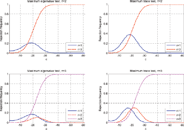
Note: Sample size is T=500. Nominal size is 5%.
Footnotes
* We are grateful to Meredith Beechey, Lennart Hjalmarsson and Randi Hjalmarsson for valuable comments on this paper and to Benjamin Chiquoine for excellent research assistance. sterholm gratefully acknowledges financial support from Jan Wallanders and Tom Hedelius foundation. The views in this paper are solely the responsibility of the authors and should not be interpreted as reflecting the views of the Board of Governors the Federal Reserve System or of any other person associated with the Federal Reserve System. Return to text
♣ Division of International Finance, Federal Reserve Board, Mail Stop 20, Washington, DC 20551, USA, email: [email protected] Phone: +1 202 452 2426. Return to text
# Department of Economics, Uppsala University, Box 513, 751 20 Uppsala, Sweden, e-mail: [email protected] Phone: +1 202 378 4135. Return to text
1. For studies relying on cointegration methods, see, for instance, Wallace and Warner (1993), Malley and Moutos (1996), Cardoso (1998), Bremnes et al. (2001), Jonsson (2001), Khamis and Leone (2001) and Bagchi et al. (2004). Studies arguing the stationarity of these variables include Song and Wu (1997, 1998), Taylor and Sarno (1998), Wu and Chen (2001) and Basher and Westerlund (2006). Return to text
2. Phillips (1988) considers both processes that have roots smaller than unity ("strongly autoregressive") and larger than unity ("mildly explosive") in his analysis of near-integrated processes. In this paper, however, we only consider the empirically most relevant case of processes with roots less than unity. Return to text
3. For a detailed description of the procedure, see, for example, Johansen (1995). Return to text
4. Based on previous studies - see, for example, Elliott, 1998 - it is no far stretch to conjecture that the Brownian motions in the limiting distribution given in, for instance, Johansen (1988) equation (18) would simply be replaced by the corresponding Ornstein-Uhlenbeck process to which near-unit-root variables converge. As always with near-unit-root variables, the problem is that the local-to-unity parameter is unknown and thus also the percentiles of the limiting distribution. Return to text
5. This means that the Johansen test can be used as a panel unit root test as suggested by Taylor and Sarno (1998) and Österholm (2004). Return to text
6. See, for example, Clark and MacDonald (1999) for a discussion of estimation of equilibrium real exchange rates. Return to text
7. One way of viewing tests of such
restictions is as unit-root tests within the VAR. Thus, if the
first stage rank test is a form of overall panel test of the
unit-root assumption in the data, the tests on the cointegrating
vector act as supplementary unit-root tests in the cases where
either a full set of unit-roots is not found (that is, ![]() or where stationarity of the entire system (that is,
or where stationarity of the entire system (that is,
![]() is not found. Return to text
is not found. Return to text
8. It should be stressed that specification tests on the cointegrating vector are also biased when the variables have near-unit-roots; see Elliott (1998). This may potentially reduce the usefulness of these additional specification tests but does not invalidate them as robustness checks. Return to text
9. This range for ![]() covers
most of the plausible values documented in the literature; see, for
example, Stock (1991) and Campbell and Yogo (2006). Return to text
covers
most of the plausible values documented in the literature; see, for
example, Stock (1991) and Campbell and Yogo (2006). Return to text
10. An alternative viewpoint is that the
problem arising from near integrated variables is one of power
rather than size, and that whenever ![]() the
correct conclusion is
the
correct conclusion is ![]() . However, in empirical
applications, cointegration tests are typically used to evaluate
whether there is a relation between the variables in the system -
not to test whether all variables in the system are stationary -
and we accordingly believe that it is most relevant to view the
issue as a matter of size. In our subsequent analysis, we will also
test for the outcome
. However, in empirical
applications, cointegration tests are typically used to evaluate
whether there is a relation between the variables in the system -
not to test whether all variables in the system are stationary -
and we accordingly believe that it is most relevant to view the
issue as a matter of size. In our subsequent analysis, we will also
test for the outcome ![]() in order to improve the
overall size properties of the test, as discussed in detail in the
main text. Return to text
in order to improve the
overall size properties of the test, as discussed in detail in the
main text. Return to text
11. Stationary inflation but integrated nominal interest rate is consistent with a unit root in the real interest rate. Support for a unit root in the real interest rate can be found in, for example, Rose (1988). Return to text
This version is optimized for use by screen readers. Descriptions for all mathematical expressions are provided in LaTex format. A printable pdf version is available. Return to text