Skip to: [Printable Version (PDF)]

Board of Governors of the Federal Reserve System
International Finance Discussion Papers
Number 919, February 2008--- Screen Reader Version*

Optimal Fiscal and Monetary Policy in Customer Markets

David M. Arseneau^† and Sanjay K. Chugh^‡

NOTE: International Finance Discussion Papers are preliminary materials circulated to stimulate discussion and critical comment. References in publications to International Finance Discussion Papers (other than an acknowledgment that the writer has had access to unpublished material) should be cleared with the author or authors. Recent IFDPs are available on the Web at http://www.federalreserve.gov/pubs/ifdp/. This paper can be downloaded without charge from the Social Science Research Network electronic library at http://www.ssrn.com/.

Abstract:

A growing body of evidence suggests that ongoing relationships between consumers and firms may be important for understanding price dynamics. We investigate whether the existence of such customer relationships has important consequences for the conduct of both long-run and short-run policy. Our central result is that when consumers and firms are engaged in long-term relationships, the optimal rate of price inflation volatility is very low even though all prices are completely flexible. This finding is in contrast to those obtained in first-generation Ramsey models of optimal fiscal and monetary policy, which are based on Walrasian markets. Echoing the basic intuition of models based on sticky prices, unanticipated inflation in our environment causes a type of relative price distortion across markets. Such distortions stem from fundamental trading frictions that give rise to long-lived customer relationships and makes pursuing inflation stability optimal.

Keywords: Inflation stability, Ramsey model, search models

JEL classification: E30, E50, E61, E63

1  Introduction

A growing body of evidence suggests that ongoing relationships between consumers and firms may be important for understanding price dynamics. In this paper, we investigate whether the existence of such customer relationships has important consequences for the conduct of both long-run and short-run policy. We explore this question using the Ramsey framework of optimal fiscal and monetary policy, in the tradition of Lucas and Stokey (1983) and Chari, Christiano, and Kehoe (1991), because it is a powerful laboratory for uncovering properties of optimal policy. Our central result is that long-term relationships between consumers and firms, which we model using search-based frictions in goods markets, make keeping inflation variability low an important goal of policy. This finding is in contrast to first-generation Ramsey models, which are based on Walrasian markets and thus are ill-suited to handle long-lived relationships. Our results are very similar to those delivered by virtually any model with nominal rigidities, even though all prices in our environment are completely flexible and not subject to any menu costs.

The basic reason that any model with nominal rigidities recommends inflation stability as the optimal policy is that variations in inflation affect relative prices of goods. Given technologically identical goods -- as virtually all sticky-price-based models assume -- it is transparent that allowing relative prices to deviate from unity as a result of variations in inflation is welfare-reducing. Hence the prescription to stabilize inflation. As a general tenet, we think this core intuition recommending inflation stability is sound. Our model and results show, however, that one does not need a typical sticky-price model to reach this prediction. In the model we use to study optimal policy, fundamental trading frictions lead to some goods being purchased in the context of long-term customer relationships, while other goods are purchased in the spot goods markets used as the basis for nearly all macroeconomic models. In this environment, volatile inflation induces a similar type of relative price distortion as in sticky-price models. Optimal policy thus stabilizes inflation.

Our environment builds on the quantitative search-based model of goods markets developed in Arseneau and Chugh (2007b). Their model, as does Hall's (2007) model, uses the search-and-matching framework familiar from the labor search literature as a basis for a model of goods markets. In both Arseneau and Chugh (2007b) and Hall (2007), the search frictions that both consumers and firms must overcome before goods trade can occur make customer relationships valuable to both parties. We extend Arseneau and Chugh (2007b) to a monetary environment, motivating money demand by layering over it a cash good/credit good structure, in the spirit of Lucas and Stokey (1983). In our model here, then, some search goods can be acquired only with cash, while others may be acquired using credit. As in a basic cash/credit model, there is no explicitly-modeled reason why some goods have to be purchased using cash. By situating a familiar cash/credit structure in a clearly-defined concept of customer relationships, however, we are able to show that goods trading frictions per se, even independent from those that generate an endogenous role for money, may have important consequences for policy recommendations.

Our primary result -- that realized (ex-post) inflation is quite stable over time in the face of business-cycle magnitude shocks -- is in contrast to the very volatile ex-post inflation rates found by Chari, Christiano, and Kehoe (1991) that have become the benchmark for the Ramsey monetary literature. Inflation volatility is high in the benchmark Ramsey model because surprise movements in the price level allow the government to synthesize real state-contingent debt payments from nominally risk-free government bonds without distorting relative prices. The government then need not change other, distortionary, tax rates much in response to shocks.

In our model, in contrast, real activity is distorted by ex-post inflation because inflation affects relative activity across goods markets in an inefficient manner. The inefficiency arises because (large) movements in inflation causes dispersion in the degree of market tightness -- the relative number of traders on opposite sides of the market -- across search markets. Well-known from standard search theory is that such dispersion is inefficient. Associated with this distortion in relative market tightness is a distortion in relative prices of goods across search markets -- hence we speak of inflation causing a relative-price distortion. Such an effect is one that a basic flexible-price Ramsey monetary model cannot articulate. Quantitatively, we find that the welfare cost of this relative-price distortion dominates the insurance value of generating state-contingent debt in our model, rendering inflation an order of magnitude more stable than in first-generation Ramsey models. Varying one key parameter that governs the importance of goods-trading frictions in our model allows us to trace out the spectrum between the optimal inflation volatility result of Chari, Christiano, and Kehoe (1991) and the optimal inflation stability result of a standard sticky-price model. Deep frictions underlying goods trade thus provide novel justification for the optimality of inflation stability.

Our second main result is that a deviation from the Friedman Rule of a zero net nominal interest rate may be optimal in the long run. The optimality of positive nominal interest rates is taken almost for granted by central bankers and those studying monetary policy using sticky-price-based models, in which the attendant deflation associated with the Friedman Rule is undesirable, but it is a result that usually has been difficult to obtain in flexible-price models. Two distinct reasons lead to a departure from the Friedman Rule in our model, and each connects naturally with recent results in the Ramsey literature. First, a positive nominal interest rate can be used to indirectly tax monopolistic producers' profits, a policy channel first identified by Schmitt-Grohe and Uribe (2004a). Second, a positive nominal interest rate can be used to offset inefficient search activity, similar to findings in the labor-search models of Cooley and Quadrini (2004) and Arseneau and Chugh (2007a) and the money-search model of Rocheteau and Wright (2005). As in all of these previous studies, allowing for policy instruments that directly tax monopoly profits and inefficient search activity restores the optimality of the Friedman Rule.

Other than Hall (2007) and Arseneau and Chugh (2007b), other studies have also taken the view that deeper models of relationships between consumers and firms, even if not applied to studying policy issues, may be important for understanding price dynamics. Such a view is motivated by the survey evidence of, for example, Blinder et al (1998) and Fabiani et al (2006), that firms often try to avoid upsetting their existing customers when considering price changes. Recent theoretical models that fall into this broadly-defined area are the deep habits models of Ravn, Schmitt-Grohe, and Uribe (2006) and Nakamura and Steinsson (2007) and the switching-cost model of Kleschelski and Vincent (2007). The main way in which our framework, along with Hall's (2007), differs from these other frameworks is that we embed customer relationships as a feature of the trading structure of the environment, rather than altering preferences to account for them. We also differ here, of course, in emphasis, using our framework to study optimal policy.

The Lucas and Stokey (1983) and Chari, Christiano, and Kehoe (1991) studies -- henceforth LS and CCK, respectively -- are the benchmark for Ramsey models of optimal fiscal and monetary policy. The LS/CCK framework is particularly effective at uncovering the welfare consequences of stabilizing inflation over the business cycle, an issue about which central bankers have strong priors. In a recent outburst of work in this area, Schmitt-Grohe and Uribe (2004a, 2004b, 2005), Siu (2004), and Chugh (2006, 2007) enrich the original Walrasian-based LS and CCK models along a number of dimensions, with a focus on studying the dynamics of optimal inflation. However, premised as they are on a fundamentally Walrasian view of markets, the primitive desirability of inflation volatility embedded in the basic LS/CCK structure underlies them all.

In a different recent direction of the Ramsey literature, Arseneau and Chugh (2007a) and Aruoba and Chugh (2006) study the dynamics of optimal inflation when key markets feature fundamental trading frictions -- frictions underlying labor market relationships in the former, and frictions underlying monetary trade in the latter. Our work here continues the theme begun in these two studies by employing a deeper description of trade in goods markets. Taken together, this emerging second generation of Ramsey models uncovers several novel insights regarding the economic forces that may shape policy, in particular monetary policy.

Although we use the canonical Ramsey framework of optimal taxation, the primary goal we set out to achieve is not the design of an efficient tax system. That is obviously one natural -- and the original -- objective to pursue using the Ramsey framework. Our model of course does have implications for optimal (regular) fiscal policy, the most basic being an echo of the standard Ramsey prescription of smoothing proportional labor tax rates over time. Instead, our primary goal here is to shed some light on how conventional thinking regarding the forces affecting monetary policy may be quite different once one treats non-Walrasian frictions in goods markets seriously, which we can isolate from a serious treatment of frictions underlying monetary trade. As second-generation and the most recent of the first-generation Ramsey monetary models have demonstrated, and as we mentioned at the outset, the Ramsey laboratory is effective at isolating such forces; Chugh (2007b) provides more discussion on this point.

The rest of our work is organized as follows. Section 2 lays out our model, which is a cash/credit version of the search-based model of goods markets developed in Arseneau and Chugh (2007b). Section 3 presents the Ramsey problem, and Section 4 presents and analyzes our steady-state and dynamic results. Section 5 summarizes and offers possible avenues for continued research.

2  The Economy

The environment builds on Arseneau and Chugh (2007b), which posits that, for some goods trades, households and firms each have to expend time and resources finding individuals on the other side of the market with whom to trade. A fraction of goods market exchange is thus explicitly bilateral, in contrast to all trades happening against the anonymous Walrasian auctioneer. The modeling device used by Arseneau and Chugh (2007b) and Hall (2007) to tractably capture these search frictions in goods markets is to adapt the aggregate matching function ubiquitous in the labor search literature.

To motivate money demand, we build on this idea by imposing a LS/CCK type of cash/credit margin on top of the search markets. Our model of money demand is as simple as existing cash/credit structures, and we think this makes our results readily comparable with most existing optimal-policy studies. We proceed to describe in turn the environment faced by households, the environment faced by firms, the determination of prices, aggregate matching dynamics, the nature of the consolidated fiscal-monetary government, and the private-sector equilibrium. At the end of the presentation of the household side of the model, we discuss the intuition for why the dynamics of Ramsey-optimal inflation have the potential to be quite different in our environment than in a baseline LS/CCK model.

2.1  Households

There is a measure one of identical, infinitely-lived households in the economy, each composed of a measure one of individuals. In a given period, an individual member of the representative household can be engaged in one of six activities: purchasing goods (shopping) at a cash location, purchasing goods (shopping) at a credit location, searching for cash goods, searching for credit goods, working, or enjoying leisure. More specifically, $l_{t}$ members of the household are working in a given period; $s_{1t}$ ($s_{2t})$ members are searching for firms from which to buy cash (credit) goods; $N^{h}_{1t}$ ( $N^{h}_{2t}$) members are shopping at firms with which they previously formed cash (credit) relationships; and $1 - l_{t} - s_{1t} - s_{2t} - N^{h}_{1t} - N^{h}_{2t}$ members are enjoying leisure.

We make more precise the distinction between cash shoppers and credit shoppers below; for now, note our more general distinction between shopping and searching for goods. Individuals who are searching are looking to form relationships with firms, which takes time. Individuals who are shopping were previously successful in forming customer relationships, but the act of acquiring and bringing home goods itself takes time.¹ We assume that all members of a household share equally the consumption that shoppers acquire.

Defining $N^{h}_{t} = N^{h}_{1t} + N^{h}_{2t}$ and $s_{t} = s_{1t} + s_{2t}$, the household's discounted lifetime utility is given by

$$E_{0} \sum_{t=0}^{\infty} \beta^{t} \left[ u(x_{1t}, x_{2t}) + \vartheta v\left( \int_{0}^{N^{h}_{1t}} c_{i1t} di, \int_{0} ^{N^{h}_{2t}} c_{i2t} di \right) + g(1-l_{t}-s_{t}-N^{h}_{t}) \right] ,$$ (1)

where $x_{1}$ is consumption of a standard Walrasian cash good, $x_{2}$ is consumption of a standard Walrasian credit good, and $c_{i1t}$ and $c_{j2t}$ are the quantities of the search cash and search credit good, respectively, that cash shopper $i$ and credit shopper $j$ bring back to the household. Instantaneous utility of leisure is $g(.)$, and the parameter $\vartheta$ governs how the household prefers to divide its total consumption between search and non-search goods.

As in Arseneau and Chugh (2007b), note that consumption of search goods potentially has two dimensions: an extensive margin (the number of cash (credit) shoppers that buy goods) and an intensive margin (the number of cash (credit) goods that each cash (credit) shopper buys). Given the complexity of our model and to keep the focus on the extensive margin of search consumption, we close down adjustment at the intensive margin and assume that the intensive quantity of either cash or credit goods obtained in a match is always $\bar{c} = 1$. Arseneau and Chugh (2007b) show the technical details one requires to open up the intensive margin; extending those requirements to our more complicated environment here is straightforward in principle, but we refrain from doing so to illustrate as clearly as possible how some conventional thinking regarding policy may change due to the presence of just the search (extensive) margin of consumption. However, we keep the notation general and continue writing $c_{ijt}$, but it will be understood from here on that $c_{ijt} = \bar{c} = 1$ $\forall i,j,t$.

The household faces the sequence of flow budget constraints,

$$\lefteqn{M_{t} - M_{t-1} + B_{t} - R_{t-1} B_{t-1} = }$$ (2)

$$(1-\tau^{l}_{t-1})W_{t-1} l_{t-1} - P_{t-1} x_{1t-1} - P_{t-1} x_{2t-1} - \int_{0}^{N^{h}_{1t-1}} P_{i1t-1} c_{i1t-1} di - \int_{0}^{N^{h}_{2t-1}} P_{i2t-1} c_{i2t-1} di + P_{t-1} d_{t-1},$$

where $M_{t-1}$ is the nominal money the household brings into period $t$, $B_{t-1}$ is nominal bonds brought into period $t$, $P_{t}$ is the nominal price level (equivalently, the nominal price of both Walrasian cash and Walrasian credit goods), $R_{t}$ is the gross nominal interest rate on nominally risk-free government bonds held between $t$ and $t+1$, $\tau^{l} _{t}$ is the tax rate on labor income, and $d_{t}$ is real dividends distributed lump-sum by firms to households. All of these objects are standard in the line of cash/credit models begun by LS and CCK and recently used by Siu (2004), Chugh (2006, 2007a), and Arseneau and Chugh (2007a). Finally, the nominal prices of cash search goods and credit search goods purchased by cash shopper $i$ and credit shopper $j$, respectively, are $P_{i1t}$ and $P_{j2t}$.

The household also faces the sequence of cash-in-advance constraints,

$$P_{t} x_{1t} + \int_{0}^{N^{h}_{1t}} P_{i1t} c_{i1t} di \leq M_{t},$$ (3)

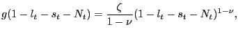
that apply to both a subset of Walrasian goods and a subset of search goods. As in LS, CCK, and the subsequent literature, the purchase of some goods requires the use of money for an unstated reason; it is a reduced-form way of motivating money demand. We extend this idea to cover both a subset of standard Walrasian goods and a subset of goods acquired via ongoing customer relationships. We point out that these ideas are quite different from those emphasized by Lagos and Wright (2005) and the related literature, in which search-type frictions in some goods trades lead endogenously to a welfare-enhancing role for fiat money. That is not the case here, as we do not use search frictions to motivate a fundamental role for money.² We interpret our setup as one that separates search frictions in goods markets from the (to use a term favored in the money-search class of models) "essentiality" of money central to money-search-based models like Lagos and Wright (2005). Our cash in advance constraint, applied to both search and non-search goods, nevertheless forms the basis of our central hypothesis that inflation variability is undesirable in the environment we study; we discuss this hypothesis further after we complete our description of the household problem.

Apart from the obvious differences due to our inclusion of search markets, the timing of both the budget constraints and cash-in-advance constraints conforms to that of LS and CCK and the ensuing literature. In addition to these constraints, the representative household also faces perceived laws of motion for the numbers of active cash customer relationships and credit customer relationships in which it is engaged,

$$N^{h}_{1t+1} = (1-\rho^{x}) ( N^{h}_{1t} + s_{1t} k^{h}(\theta_{1t}) )$$ (4)

and

$$N^{h}_{2t+1} = (1-\rho^{x}) ( N^{h}_{2t} + s_{2t} k^{h}(\theta_{2t}) ).$$ (5)

The probability that a searching individual forms a cash (credit) relationship is $k^{h}$, which in turn depends on aggregate market tightness $\theta_{1}$ ( $\theta_{2}$) in cash (credit) search markets. Market tightness, defined as the aggregate number of advertisements per searching individual in a given market, is taken as given by the household, hence matching probabilities are taken as given by the household. With fixed probability $\rho^{x}$, which is known to both households and firms, an existing customer relationship dissolves at the beginning of a period.³

This completes the basic description of the environment households face. We relegate more formal details of the household optimization problem to Appendix A; we proceed here directly to the optimality conditions. Before presenting household optimality conditions, a few points are in order. First, we restrict attention to equilibria that are symmetric across all cash relationships and symmetric across all credit relationships -- that is, $P_{i1t} = P_{i^{\prime}1t} = P_{1t}$ $\forall$ $i \neq i^{\prime}$ and $P_{j2t} = P_{j^{\prime}2t} = P_{2t}$ $\forall$ $j \neq j^{\prime}$. Second, define $p_{1t} \equiv P_{1t} / P_{t}$ and $p_{2t} \equiv P_{2t} / P_{t}$ as the symmetric equilibrium relative prices of search cash and search credit goods, respectively. Third, to conserve on notation, from here on let $v_{it}$ stand for $v_{i}\left( \int_{0}^{N^{h}_{1t}} c_{i1t} di, \int_{0}^{N^{h}_{2t}} c_{i2t} di \right)$ , $g^{\prime}_{t}$ stand for $g^{\prime}(1-l_{t}-s_{t}-N^{h}_{t})$, and $u_{it}$ stand for $u_{i}(x_{1t}, x_{2t})$

Three household optimality conditions are identical to those in standard cash/credit models: the consumption-leisure optimality condition

$$\frac{g^{\prime}_{t}}{u_{2t}} = (1-\tau ^{l}_{t}) w_{t},$$ (6)

the (Walrasian) cash-good/credit-good optimality condition

$$\frac{u_{1t}}{u_{2t}} = R_{t},$$ (7)

and an Euler equation that prices a one-period nominally risk-free bond

$$1 = R_{t} E_{t} \left[ \frac{\beta u_{1t+1}}{u_{1t}} \frac {1}{\pi_{t+1}} \right] ,$$ (8)

where $\pi_{t} \equiv P_{t} / P_{t-1}$ is the gross inflation rate between periods $t-1$ and $t$.

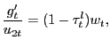
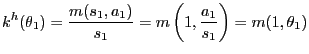
In search markets, the household's choice of $s_{it}$ to hit a target $N^{h}_{it+1}$ make shopping decisions akin to investment decisions, just as in Arseneau and Chugh (2007b) and Hall (2007). The optimal shopping condition for cash goods is

$$\frac{g^{\prime}_{t}}{k^{h}(\theta_{1t})} = \beta(1-\rho^{x}) E_{t} \left\{ c_{1t+1} \left[ \vartheta v_{1t+1} - p_{1t+1} u_{1t+1} \right] - g^{\prime}_{t+1} + \frac{g^{\prime}_{t+1}}{k^{h} (\theta_{1t+1})} \right\} ,$$ (9)

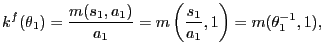
and the optimal shopping condition for credit goods is

$$\frac{g^{\prime}_{t}}{k^{h}(\theta_{2t})} = \beta(1-\rho^{x}) E_{t} \left\{ c_{2t+1} \left[ \vartheta v_{2t+1} - p_{2t+1} u_{2t+1} \right] - g^{\prime}_{t+1} + \frac{g^{\prime}_{t+1}}{k^{h} (\theta_{2t+1})} \right\} .$$ (10)

The cash (credit) shopping condition simply states that at the optimum, the household sends a number of individuals out to search for cash (credit) goods such that the expected marginal cost of shopping for a cash (credit) good equals the expected marginal benefit of forming a cash (credit) relationship. The expected marginal benefit of a cash (credit) relationship is composed of two parts: the utility gain from obtaining $c_{1t}$ ($c_{2t}$) more cash (credit) goods via the search market rather than via the Walrasian market (net of the direct disutility $g^{\prime}$ of shopping) and the asset value to the household of having one additional pre-existing cash (credit) customer relationship entering period $t+1$.

Because it will be useful in understanding our optimal policy results, note that the shopping conditions (9) and (10) can be condensed into a household shopping margin,

$$\frac{E_{t} \left\{ c_{1t+1} \left[ \vartheta v_{1t+1} - p_{1t+1} u_{1t+1} \right] - g^{\prime}_{t+1} + \frac{g^{\prime}_{t+1}}{k^{h}(\theta_{1t+1})} \right\} } {E_{t} \left\{ c_{2t+1} \left[ \vartheta v_{2t+1} - p_{2t+1} u_{2t+1} \right] - g^{\prime }_{t+1} + \frac{g^{\prime}_{t+1}}{k^{h}(\theta_{2t+1})} \right\} } = \frac{k^{h}(\theta_{2t})}{k^{h}(\theta_{1t})},$$ (11)

which emphasizes that, when sending members out to shop for goods, the household faces a cash-search/credit-search decision margin. The relevant "price" influencing this margin is relative matching probabilities. The higher is the matching probability $k^{h}(\theta_{2t})$ in the credit market, the more costly it is, ceteris paribus, for a household to assign an additional member to search in the cash market. Furthermore, because we assume Cobb-Douglas matching technologies, the relative matching probability depends only on relative market tightness, $\theta_{1t}/\theta_{2t}$. From the point of view of the Ramsey government, then, relative market tightness is a "price" that can be manipulated. As we point out when we discuss how $p_{1t}$ and $p_{2t}$ are determined, $\theta_{it}$ and $p_{it}$, $i=1,2$ are tightly linked, as is well-understood in standard search theory. Hence, $\theta _{1t}/\theta_{2t}$ is closely-linked to $p_{1t}/p_{2t}$, which is why we refer to $\theta_{1t}/\theta_{2t}$ as a relative price.

We now return to a point we mentioned earlier: our central hypothesis can be seen in our model's cash-in-advance constraint. As in nearly all cash-in-advance models, we focus on an equilibrium in which the cash-in-advance constraint binds. In a symmetric equilibrium, the time-$t$ and $t-1$ versions of (3) can thus be combined to yield

$$\pi_{t} \left[ \frac{x_{1t} + p_{1t} N_{1t} c_{1t} }{x_{1t-1} + p_{1t-1} N_{1t-1} c_{1t-1}} \right] = \mu_{t},$$ (12)

where $\mu_{t} \equiv M_{t} / M_{t-1}$ is the gross growth rate of the nominal money stock. If there were no search frictions, this would reduce to $\pi_{t} (x_{1t}/x_{1t-1}) = \mu_{t}$, the standard condition relating inflation to money growth in cash-in-advance models. In a deterministic steady state, the monetarist condition $\pi= \mu$ pins down inflation. Despite search frictions, the simple monetarist relation obviously continues to hold in the steady state of our model. But dynamics in the search market complicate the dynamic relationship between fluctuations in money growth and inflation. In particular, and this forms the basis for the central hypothesis of our project, note that (12) links realized inflation $\pi_{t}$ to the relative price $p_{1t}$. Fluctuations in $\pi_{t}$ thus have the potential to transmit into fluctuations in $p_{1t}$, which in turn may disrupt search markets. This means that state-contingent movements in $\pi_{t}$ under the Ramsey plan may be undesirable in a way that does not occur in a baseline LS/CCK model. We can only assess this conjecture quantitatively.

Finally, define

$$\Xi_{t+1\vert t} = \frac{\beta u_{2t+1}}{u_{2t}}$$ (13)

as the conditional real discount factor between period $t$ and $t+1$, which will be useful in constructing firms' optimization problems, to which we turn next.

2.2  Walrasian Firms

To make pricing labor simple, we assume that there is a representative firm that buys labor in and sells the Walrasian goods $x_{1}$ and $x_{2}$ in competitive spot markets. The firm operates a linear production technology subject to aggregate TFP fluctuations. Profit-maximization yields the standard results that the real wage is equated to the marginal product of labor,

$$w_{t} = z_{t},$$ (14)

where $z_{t}$ is the period-$t$ realization of aggregate TFP. All participants in the economy, including the non-Walrasian firms described next, take this $w_{t}$ as given.

2.3  Non-Walrasian Firms

There is a measure one of identical firms that sell goods through bilateral relationships with customers. Bilateral relationships are classified as either cash relationships or credit relationships, and a given relationship is always one or the other for as long as it remains intact. For each good that it sells through either a cash or a credit relationship, the firm must first attract a customer. To attract customers, the firm must advertise, and how any given level of cash (credit) advertisements it posts maps into how many cash (credit) customers it finds is governed by matching technologies to be described below. Owing to frictions associated with finding customers, be they cash customers or credit customers, the firm views existing customers as assets. Its total stocks of cash customers and credit customers evolve according to the perceived laws of motion

$$N^{f}_{1t+1} = (1-\rho^{x}) (N^{f}_{1t} + a_{1t} k^{f}(\theta_{1t}))$$ (15)

and

$$N^{f}_{2t+1} = (1-\rho^{x}) (N^{f}_{2t} + a_{2t} k^{f}(\theta_{2t})),$$ (16)

which are obviously analogous to the customer laws of motion facing households; $k^{f}$ denotes a firm's probability of attracting a customer through an advertisement, which in turn depends on the aggregate tightness of the market in which the advertisement is placed.

As with competitive firms, search firms' production technology is linear in labor and subject to aggregate productivity $z_{t}$. Because we assume a constant-returns production technology with no fixed costs of production (there is a fixed cost of advertising, but no fixed cost of producing), its real marginal cost of production is constant and coincides with average cost. Denoting period-$t$ marginal production cost by $mc_{t}$, we can express the firm's total production costs as the sum of production costs across all of its active customer relationships, $\int_{0}^{N^{f}_{1t}} mc_{t} c_{i1t} di + \int_{0}^{N^{f}_{2t}} mc_{t} c_{i2t} di$ .

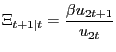
With this structure in place, total nominal profits of the representative search firm in a given period $t$ are

$$\int_{0}^{N^{f}_{1t}} P_{i1t} c_{i1t} di + \int_{0}^{N^{f}_{2t}} P_{i2t} c_{i2t} di - \int_{0}^{N^{f}_{1t}} P_{t} mc_{t} c_{i1t} di - \int_{0} ^{N^{f}_{1t}} P_{t} mc_{t} c_{i1t} di - P_{t} \gamma(a_{1t} + a_{2t}),$$ (17)

where $\gamma$ is the flow cost of posting an advertisement in either the cash market or the credit market.⁴The firm's customer bases $N^{f}_{1t}$ and $N^{f}_{2t}$ are pre-determined entering period $t$. Discounted lifetime nominal profits of the firm are thus

$$E_{0} \sum_{t=0}^{\infty} \left( \Xi_{t\vert}\frac{P_{0} }{P_{t+1}}\right) \left[ \int_{0}^{N^{f}_{1t}} P_{i1t} c_{i1t} di + \int _{0}^{N^{f}_{2t}} P_{i2t} c_{i2t} di - \int_{0}^{N^{f}_{1t}} P_{t} mc_{t} c_{i1t} di - \int_{0}^{N^{f}_{2t}} P_{t} mc_{t} c_{i2t} di - P_{t} \gamma(a_{1t} + a_{2t}) \right] ,$$ (18)

where $\left( \Xi_{t\vert} \frac{P_{0}}{P_{t+1}} \right)$ is the period-0 value to the household of a period-$t$ nominal unit, which we assume the firm uses to discount nominal profit flows because households are the ultimate owners of firms.⁵

Firms maximize (18) subject to the customer evolution constraints (15) and (16) by choosing $\left\{ a_{1t}, a_{2t}, N^{f}_{1t+1}, N^{f}_{2t+1} \right\}$. Optimization leads to what we refer to (following Arseneau and Chugh (2007b)) as the firm's optimal advertising conditions: one for advertising in cash markets,

$$\frac{\gamma}{k^{f}(\theta_{1t})} = (1-\rho^{x}) E_{t} \left\{ \Xi_{t+1\vert t} \left( p_{1t+1} c_{1t+1} - mc_{t+1} c_{1t+1} + \frac{ \gamma}{k^{f}(\theta_{1t+1})} \right) \right\} ,$$ (19)

and one for advertising in credit markets,

$$\frac{\gamma}{k^{f}(\theta_{2t})} = (1-\rho^{x}) E_{t} \left\{ \Xi_{t+1\vert t} \left( p_{2t+1} c_{2t+1} - mc_{t+1} c_{2t+1} + \frac{ \gamma}{k^{f}(\theta_{2t+1})} \right) \right\} .$$ (20)

The term $\Xi_{t+1\vert t} \equiv\Xi_{t+1\vert} / \Xi_{t\vert}$ is the household real discount factor (again, technically, the real interest rate) between period $t$ and $t+1$. In equilibrium, $\Xi_{t+1\vert t} = \frac{\beta E_{t+1} \phi_{t+2} }{E_{t} \phi_{t+1}}$ , which in turn by the household's optimal choice of Walrasian credit goods, is $\Xi_{t+1\vert t} = \frac{\beta u_{2t+1}}{u_{2t}}$ -- see Appendix A for more details. In writing (19) and (20), we have imposed symmetry across all cash relationships and across all credit relationships.

Finally, a firm's allocation of total advertising across cash and credit markets is described by

$$\frac{E_{t} \left\{ \Xi_{t+1\vert t} \left( p_{1t+1} c_{1t+1} - mc_{t+1} c_{1t+1} + \frac{ \gamma}{k^{f} (\theta_{1t+1})} \right) \right\} } {E_{t} \left\{ \Xi_{t+1\vert t} \left( p_{2t+1} c_{2t+1} - mc_{t+1} c_{2t+1} + \frac{ \gamma}{k^{f}(\theta_{2t+1})} \right) \right\} } = \frac{k^{f}(\theta_{2t})}{k^{f}(\theta_{1t})},$$ (21)

obtained by combining (19) and (20). Just like condition (11), the allocation of activity across cash search and credit search markets is governed only by $\theta _{1t}/\theta_{2t}$ due to our assumption that matching functions are Cobb-Douglas.

2.4  Price Determination

Because it is widely-understood, we employ Nash bargaining over price in both cash relationships and credit relationships as the price-determination mechanism. Appendix B provides the details behind the solutions that we present here. The relative prices $p_{1t}$ and $p_{2t}$ of cash search goods and credit search goods, respectively, that emerge from Nash bargaining are

$$p_{1t} c_{1,t} = (1-\eta) \left( \frac{\tilde {v}^{1}(c_{1t})}{\beta E_{t} \phi_{t+1} + \lambda_{t}} \right) + \eta(mc_{t} c_{1,t} - \gamma\theta_{1t})$$ (22)

and

$$p_{2t} c_{2,t} = (1-\eta) \left( \frac{\tilde {v}^{2}(c_{2t})}{\beta E_{t} \phi_{t+1}} \right) + \eta(mc_{t} c_{2,t} - \gamma\theta_{2t}),$$ (23)

where $\eta$ is the Nash bargaining power of customers in both cash and credit relationships. The total payment $p_{it} c_{it}$ a customer hands over to a firm is a convex combination of the customer's valuation of the goods obtained (given by the first terms in parentheses on the right-hand-side of (22) and (23)) and the firm's effective marginal cost of selling those goods (given by the second terms in parentheses on the right-hand-side of (22) and (23)), which takes into account both the production cost and the resources spent finding the customer in the first place. The function $\tilde{v}^{1}(.)$ is the marginal utility to the household of obtaining cash consumption from the $i$-th match, and $\tilde {v}^{2}(.)$ is the marginal utility to the household of obtaining credit consumption from the $i$-th match. Hence, $\tilde{v}^{i}(.) \equiv v_{it}(.)$, $i = 1,2$.

The main difference between (22) and (23) is in the factor by which the household discounts $\tilde{v}^{i}(.)$. Let $\phi_{t}/P_{t-1}$ denote the Lagrange multiplier on the household's budget constraint (2) and $\lambda_{t} / P_{t}$ the Lagrange multiplier on the cash-in-advance constraint (3). Because cash must be used, by definition, for cash relationships, the relevant discount takes into account both these multipliers. For credit relationships, only the multiplier on the wealth constraint is relevant because cash does not need to be held. In equilibrium, by the household first-order conditions on Walrasian cash goods and Walrasian credit goods (presented in Appendix A), $\beta E_{t} \phi_{t+1} = u_{2t}$ and $\beta E_{t} \phi_{t+1} + \lambda_{t} = u_{1t}$, which are standard in cash/credit models.⁶ Recalling condition (7), these equilibrium relations mean that the nominal interest rate $R_{t}$ implicitly affects the price ratio $p_{1t} / p_{2t}$.

2.5  Goods Market Matching

The numbers of new customer-firm cash relationships and credit relationships that form in any period $t$ are described by a pair of aggregate matching functions $m^{1}(s_{1t}, a_{1t})$ and $m^{2}(s_{2t}, a_{2t})$. We assume symmetry across the matching technologies (although we again point out that one could relax this assumption), so from here on we write $m(.) = m^{1}(.) = m^{2}(.)$. As is standard in a Mortensen-Pissarides type of framework, the matching technology is Cobb-Douglas, $m(s_{t}, a_{t})$. With Cobb-Douglas matching, the probabilities that shoppers and firms, respectively, find partners in the cash market are

$$k^{h}(\theta_{1}) = \frac{m(s_{1}, a_{1})}{s_{1}} = m\left( 1, \frac{a_{1}}{s_{1}}\right) = m(1, \theta_{1})$$ (24)

and

$$k^{f}(\theta_{1}) = \frac{m(s_{1}, a_{1})}{a_{1}} = m\left( \frac{s_{1}}{a_{1}}, 1\right) = m(\theta_{1}^{-1}, 1),$$ (25)

with $\theta_{1} \equiv a_{1}/s_{1}$ a measure of how tight (the ratio of firms searching for customers to individuals searching for goods in the cash market) the cash goods market is. Matching probabilities and market tightness in the credit search market are defined in the obvious way, with $s_{2}$ replacing $s_{1}$, $a_{2}$ replacing $a_{1}$, and $\theta_{2}$ replacing $\theta_{1}$.

As in the labor search literature and as adapted by Hall (2007) and Arseneau and Chugh (2007b), the matching function is meant to be a reduced-form way of capturing the idea that it takes resources, be it time or otherwise, for parties on opposite sides of the market to meet. Rogerson, Shimer, and Wright (2005, p. 968) note that the ability to be agnostic about the actual mechanics of the process by which parties make contact with each other may be a virtue. Our modeling motivation is very much in line with this idea.

With the matching functions describing the flow of new customer relationships, the aggregate numbers of active cash customer relationships and credit customer relationships evolve according to

$$N_{1t+1} = (1-\rho^{x}) (N_{1t} + m(s_{1t}, a_{1t}))$$ (26)

and

$$N_{2t+1} = (1-\rho^{x}) (N_{2t} + m(s_{2t}, a_{2t})).$$ (27)

2.6  Government

The government's flow budget constraint is

$$M_{t} + B_{t} + \tau^{l}_{t-1} P_{t-1} w_{t-1} l_{t-1} = M_{t-1} + R_{t-1} B_{t-1} + P_{t-1} g_{t-1},$$ (28)

where $g_{t}$ denotes exogenous government consumption in period $t$. The government finances its spending through proportional labor income taxation, issuance of nominal one-period debt, and money creation. Note that government consumption is a credit good, following Chari, Christiano, and Kehoe (1991), because $g_{t-1}$ is not paid for until period $t$.

2.7  Resource Constraint

Cash goods and credit goods are technologically identical. Furthermore, Walrasian consumption goods and search consumption goods are also technologically identical. Hence, the only "differentiation" along both dimensions is in terms of transactions methods/trading structures. The resource constraint of the economy is thus

$$x_{1t} + x_{2t} + \int_{0}^{N_{1t}} c_{i1t} di + \int_{0}^{N_{2t}} c_{i2t} di + g_{t} + \gamma(a_{1t} + a_{2t}) = z_{t} l_{t}.$$ (29)

In symmetric equilibrium,

$$x_{1t} + x_{2t} + N_{1t} c_{1t} + N_{2t} c_{2t} + g_{t} + \gamma(a_{1t} + a_{2t}) = z_{t} l_{t}.$$ (30)

2.8  Private-Sector Equilibrium

A private-sector equilibrium is made up of endogenous processes
$\left\{ x_{1t}, x_{2t}, l_{t}, s_{1t}, s_{2t}, a_{1t}, a_{2t}, N_{1t+1}, N_{2t+1}, p_{1t}, p_{2t}, \pi_{t}, R_{t}, w_{t} \right\}$ that satisfy the household optimality conditions (6), (7), (8), (9), and (10); efficiency in the labor market (14); the firm advertising conditions (19) and (20); the Nash pricing conditions (22) and (23); the aggregate laws of motion for active cash relationships and active credit relationships (26) and (27); the government budget constraint (28); and the aggregate resource constraint (30) for given exogenous processes $\left\{ z_{t}, g_{t}, \tau^{l}_{t}, \mu_{t} \right\}$. Furthermore, the restriction $R_{t} \geq1$, which states that the net nominal interest rate cannot be less than zero, is a requirement for a monetary equilibrium. Also, as we have already pointed out, $c_{1t} = c_{2t} = \bar{c} = 1$ $\forall t$.

3  Ramsey Problem

In standard Ramsey models with flexible prices, a well-known result is that household optimality conditions can be condensed into a single, present-value implementability constraint (PVIC) that encodes all of the equilibrium conditions that, apart from the resource frontier, must be respected by Ramsey allocations. In more complicated environments, such as Schmitt-Grohe and Uribe (2004b), Chugh (2006), and Arseneau and Chugh (2007a), it is not always possible to construct a PVIC, meaning that, in principle, all of the household (and other) optimality conditions must be imposed explicitly as constraints on the Ramsey problem.

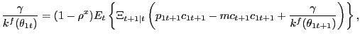
Our environment presents an intermediate case. We can construct a PVIC using the "standard" household optimality conditions (6), (7), and (8), but the household and firm optimality conditions surrounding the search markets cannot easily be captured by it. Thus, we adopt a hybrid approach, constructing a Ramsey problem that is constrained by the resource frontier, the PVIC, as well as all conditions surrounding search and pricing activities in the non-Walrasian markets. As we show in Appendix D, starting with the household flow budget constraint (2), conditions (6), (7>), and (8) can be condensed into the PVIC,

$${\small E_{0} \sum_{t=0}^{\infty} \beta^{t} \left[ u_{1t} x_{1t} + u_{2t} x_{2t} - g^{\prime}_{t} l_{t} + (u_{1t} - u_{2t}) p_{1t} N_{1t} c_{1t} + u_{2t} mc_{t} N_{1t} c_{1t} + u_{2t} mc_{t} N_{2t} c_{2t} + u_{2t} \gamma(a_{1t} + a_{2t}) \right] = A_{0}.}$$ (31)

In constructing (31), we impose a binding cash-in-advance constraint (which is standard in Ramsey analyses based on a cash/credit structure) and substitute in the symmetric equilibrium expression for real firm dividend payments, $d_{t} = (p_{1t} - mc_{t}) N_{1t} c_{1t} + (p_{2t} - mc_{t}) N_{2t} c_{2t} - \gamma(a_{1t} + a_{2t})$ . If there were no search frictions and hence no customer relationships, we would have $\gamma= N_{1} = N_{2} = 0$, in which case the PVIC would roll back to $E_{0} \sum _{t=0}^{\infty} \beta^{t} \left[ u_{1t} x_{1t} + u_{2t} x_{2t} - g^{\prime }_{t} l_{t} \right] = A_{0}$ , identical to that in LS and CCK.

The Ramsey problem is thus to choose state-contingent processes
$\{x_{1t}, x_{2t}, l_{t}, s_{1t}, s_{2t}, \theta_{1t}, \theta_{2t}, N_{1t+1}, N_{2t+1}, p_{1t}, p_{2t}\}_{t=0}^{\infty}$ to maximize (1) subject to the PVIC (31), the resource constraint (30), the household shopping conditions (9) and (10), the firm advertising conditions (19) and (20), the Nash pricing conditions (22) and (23), and the aggregate laws of motion of cash and credit customer relationships (26) and (27). By using the resource constraint and the household budget constraint (which is embedded inside (31)), we do not need to specify the government budget constraint (28) as a constraint on the Ramsey problem because it is implied. The Ramsey government takes as given the exogenous processes $\{z_{t}, g_{t}\}_{t=0}^{\infty}$. Given the Ramsey allocation, we can then construct the policy processes $\{\tau^{l}_{t}, R_{t}, \pi_{t}\}_{t=0} ^{\infty}$ using (6), (7), and (8); the Ramsey-optimal money growth rate process $\{\mu _{t}\}_{t=0}^{\infty}$ can be constructed using (12).

In principle, we must also impose the inequality condition

$$u(c_{1t}, c_{2t}) - u(c_{1t}, c_{2t}) \geq1$$ (32)

as a constraint on the Ramsey problem, which would guarantee (in terms of allocations -- refer to condition (7)) that the zero-lower-bound on the net nominal interest rate is not violated. We thus refer to constraint (32) as the ZLB constraint. The ZLB constraint in general is an occasionally-binding constraint.

Because our model likely is too complex, given current technology, to solve using global approximation methods (as we describe below, we use a locally-accurate approximation method) that would be able to properly handle occasionally-binding constraints, for our dynamic results we drop the ZLB constraint and then check whether the ZLB constraint is ever violated during simulations. For our benchmark calibration, it turns out the ZLB is never violated, meaning we are justified in dropping it. For our steady-state results, keeping the ZLB constraint in place poses no computational problem because we use a non-linear equation solver. Finally, throughout, we assume that the first-order conditions of the Ramsey problem are necessary and sufficient and that all allocations are interior.

4  Optimal Policy

We characterize both the Ramsey steady-state and dynamic policies and allocations numerically. Before turning to our results, we describe how we parameterize our model. Because our model weds a standard cash/credit foundation to a search-based view of (some) goods trades, we draw on two different literatures in choosing our baseline parameter settings. Parameters surrounding the basic cash/credit structure are drawn from LS, CCK, and Siu (2004), while the parameters surrounding search in goods markets are drawn from Arseneau and Chugh (2007b) and Hall (2007).

4.1  Parameterization

The time unit in our model is one quarter, so we set the subjective time discount factor to $\beta=0.9924$, in line with an average real interest rate of three percent. For instantaneous utility over Walrasian cash and credit goods, we choose

$$u(x_{1t}, x_{2t}) = \frac{\left\{ \left[ (1-\kappa_{x}) x_{1t}^{\phi_{x}} + \kappa_{x} x_{2t}^{\phi_{x}}\right] ^{1/\phi_{x}}\right\} ^{1-\sigma_{x}} - 1}{1-\sigma_{x}};$$ (33)

such a CES aggregate of cash and credit goods nested inside CRRA utility is standard in cash/credit models. Following Siu (2004), we set $\phi_{x} = 0.79$, and, consistent with many macro models, we set $\sigma_{x} = 1$, making utility log in the consumption aggregate. For instantaneous utility over leisure, we choose

$$g(1-l_{t}-s_{t}-N_{t}) = \frac{\zeta}{1-\nu} (1-l_{t}-s_{t}-N_{t})^{1-\nu},$$ (34)

also standard. We set $\nu= 0.4$, which makes our calibration of the elasticity of leisure with respect to the real wage consistent with most macro models; however, we point out that this does not necessarily mean that the wage elasticity of labor supply is the same as in standard models because in addition to labor and leisure, searching and shopping are part of a household's "time constraint" as well. Given the rest of our calibration, $N + s$ is much smaller than either labor or leisure, so our parameter setting seems not grossly misleading. We set $\zeta=4.3$ so that $l = 0.28$ in the deterministic Ramsey steady state of our benchmark specification.

To make preferences symmetric across Walrasian and non-Walrasian goods, instantaneous utility $v$ is

$$v\left( \int_{0}^{N_{1t}} c_{i1t} di, \int_{0}^{N_{2t}} c_{i2t} di\right) = \frac{\left\{ \left[ (1-\kappa_{c}) \left[ \int_{0}^{N_{1t}} c_{i1t} di\right] ^{\phi_{c}} + \kappa_{c} \left[ \int_{0}^{N_{2t}} c_{i2t} di\right] ^{\phi _{c}}\right] ^{1/\phi_{c}}\right\} ^{1-\sigma_{c}} - 1}{1-\sigma_{c}},$$ (35)

again a CES aggregate of cash (search) and credit (search) goods nested inside CRRA utility. Natural baseline setting are $\phi_{c} = \phi_{x} = 0.79$ and $\sigma_{c} = \sigma_{x} = 1$; to finish making $u$ and $v$ as symmetric as possible, we would want $\kappa_{c} = \kappa_{x}$. Siu (2004) estimates $\kappa_{x} = 0.62$, and this value is adopted by Chugh (2006, 2007) and Arseneau and Chugh (2007a). In the interest of making things really symmetric, however, we will set as our baseline $\kappa_{c} = \kappa_{x} = 0.5$, delivering symmetry along the cash/credit dimensions of both search goods and non-search goods; this parameter choice will help in understanding some of the core forces at work in the model. We explore sensitivity to asymmetric preferences in some of our experiments.

We set the preference parameter $\vartheta= 1$, which governs the composition of search consumption in total consumption, as a baseline. With this baseline setting and given the rest of our calibration, the fraction of total consumption that is comprised of consumption obtained through search is about 25 percent in the Ramsey equilibrium. That is, $\vartheta= 1$ delivers $\frac{N_{1} c_{1} + N_{2} c_{2}}{N_{1} c_{1} + N_{2} c_{2} + x_{1} + x_{2} }=0.25$ , which does not seem unreasonable; however, we do not have direct evidence on this share. Varying $\vartheta$ varies this share, and doing so helps illuminate some forces at work in our model, especially for our dynamic results. In the limit, $\vartheta= 0$ collapses our model to a standard LS/CCK cash/credit model in which all goods are exchanged via Walrasian trade. Our calibration also delivers $\frac{N_{1} + s_{1} + N_{2} + s_{2}}{\l } = 0.32$, meaning that households spend about one-third as much time in shopping-related activities as they do working. As discussed in Arseneau and Chugh (2007b), this is close to the evidence in the American Time Use Survey that the average individual spends about one hour in shopping activities for every four hours of work.

As we stated earlier, we choose a standard Cobb-Douglas matching function,

$$m(s,a) = \psi s^{\xi_{s}} a^{1-\xi_{s}}$$ (36)

and set the elasticity to $\xi_{s}=0.5$. We calibrate $\psi$ so that the steady-state quarterly probability a searching individual successfully forms a customer relationship is 90 percent, $k^{h} = 0.9$. For the Nash bargaining weight $\eta$, we choose $\eta= \xi_{s} = 0.5$, which has the virtue, well-known to search theorists since Hosios (1990), that it makes the underlying search equilibrium socially-efficient. We of course do not know if an efficient search equilibrium in the goods market is the best description of the data, but Hosios efficiency seems useful as a starting point for our theoretical investigation. Hosios efficiency, or the lack thereof, turns out to be one of the important forces at work in our model shaping the long-run Ramsey policy.

We set the cost $\gamma$ to a firm of posting an advertisement such that total advertising expenditures $\gamma(a_{1} + a_{2})$ absorb about four percent of output in the Ramsey equilibrium, consistent with, although a bit higher than, the evidence presented in Arseneau and Chugh (2007b) that advertising expenditures make up about 2.5 percent of GDP. The reason we calibrate a bit higher is that given our cash/credit structure, we think that some "long-term cash relationships" may be a product of relatively informal advertising expenditures that would not be recorded in the data.⁷ Finally, absent direct evidence, we simply set $\rho^{x} = 0.10$, which states that a firm loses ten percent of its existing customers in any given period. Equivalently, this parameter setting means that a newly-formed customer-firm relationship is expected to last for $1/\rho^{x} = 10$ periods (quarters), which we think does not seem implausible.

The exogenous productivity and government spending shocks follow AR(1) processes in logs,

$$\ln z_{t} = \rho_{z} \ln z_{t-1} + \epsilon^{z}_{t},$$ (37)

$$\ln g_{t} = (1-\rho_{g})\ln\bar{g} + \rho_{g} \ln g_{t-1} + \epsilon^{g}_{t},$$ (38)

where $\bar{g}$ denotes the steady-state level of government spending, which we calibrate in our baseline model to constitute 18 percent of steady-state output in the Ramsey allocation. The resulting value is $\bar{g} = 0.06$, which we hold constant as we try other specifications of our model. The innovations $\epsilon^{z}_{t}$ and $\epsilon^{g}_{t}$ are distributed $N(0, \sigma^{2}_{\epsilon^{z}})$ and $N(0, \sigma^{2}_{\epsilon^{g}})$, respectively, and are independent of each other. We choose parameters $\rho_{z} = 0.95$, $\rho_{g}=0.97$, $\sigma_{\epsilon^{z}}=0.006$, and $\sigma_{\epsilon^{g}}=0.03$, consistent with the RBC literature and CCK. Also regarding policy, we assume that the steady-state government debt-to-GDP ratio (at an annual frequency) is 0.5, in line with evidence for the U.S. economy and with the calibrations of Schmitt-Grohe and Uribe (2004b) and Siu (2004).

4.2  Ramsey Steady State

We begin by describing the deterministic Ramsey steady state, presented in the top panel of Table 1. The most interesting feature of the Ramsey policy is that the optimal nominal interest rate, at an annual rate of 5.6 percent, violates the Friedman Rule of a zero net nominal interest rate that is optimal in a wide class of models. We explain next why a deviation from the Friedman Rule occurs in our environment. In terms of allocations, however, given that a positive nominal interest rate is in place, it is quite intuitive that activity in the cash search market is depressed compared to activity in the credit search market. That is, $N$, $s$, and $a$ are all lower in the cash sector than in the credit sector. The intuition behind this result is quite simple: a positive nominal interest rate directs activity away from the cash search market and towards the credit search market, in the same way that it directs activity away from Walrasian cash-good markets and towards Walrasian credit-good markets.

Table 1:  Steady-state Ramsey and socially-efficient allocations. Nominal interest rate, inflation rate, and shadow nominal interest rate reported in annualized percentage points.

Allocation	$R-1$	$\pi-1$	$\tau^{l}$	$R^{*}-1$	$s_{1}$	$s_{2}$	$a_{1}$	$a_{2}$	$N_{1}$	$N_{2}$	$\theta_{1}$	$\theta_{2}$	$gdp$
Ramsey policy and allocation	5.6561	2.4864	0.2776	-3.4060	0.0133	0.0160	0.0156	0.0175	0.0248	0.0288	1.1718	1.0934	0.2734
Ramsey policy and allocation with 100% profit tax	3.1750	0.0797	0.1973	-1.8079	0.0140	0.0155	0.0177	0.0188	0.0270	0.0293	1.2601	1.2149	0.2929
Ramsey policy and allocation with 100% profit tax and search tax	0	-3	0.1648	0	0.0126	0.0126	0.0191	0.0191	0.0266	0.0266	1.5097	1.5097	0.2995
Socially-efficient allocation	0	-3	0	0	0.0146	0.0146	0.0221	0.0221	0.0308	0.0308	1.5135	1.5135	0.3372

In order to understand the sub-optimality of the Friedman Rule, it is crucial to first understand the consequences of a positive labor income tax rate in our model because, as must be the case in a non-trivial Ramsey policy, we have $\tau^{l} > 0$. As we demonstrate in detail in Appendix E, a labor income tax distorts not only labor supply in our model, but also household shopping behavior because shopping and leisure are both alternatives to labor as uses of a household's time. As in any standard model, ceteris paribus, a positive labor income tax rate causes households to substitute out of labor, $l$, and into leisure, which in our model is $1-l-s_{1}-s_{2}-N_{1}-N_{2}$. The resulting decline in the marginal utility of leisure, $g^{\prime }(1-l-s_{1}-s_{2}-N_{1}-N_{2})$, means that the cost of engaging in additional search activity falls as well, inducing households to spend more time searching for goods.⁸ Thus, even though the typical Hosios parameterization for search efficiency ( $\eta= \xi_{s}$) is in place in our model, household search activity is inefficiently high. This type of labor-tax-policy-induced violation of Hosios-efficiency was first described by Arseneau and Chugh (2006).

With this understanding of how $\tau^{l}$ influences shopping behavior, a strictly positive net nominal interest rate $R-1$ has three effects in our model. One effect of $R>1$ is the standard wedge created in the margin between Walrasian cash goods $x_{1}$ and Walrasian credit goods $x_{2}$. A second effect is that $R>1$ plays a role in guiding search markets towards their Hosios-efficient outcomes. Specifically, as we pointed out above, higher levels of $R$ direct household search activity away from the cash sector and towards the credit sector. This novel effect of a positive nominal interest rate mitigates part of the inefficiently-high search behavior induced by $\tau^{l} > 0$ and is one of the reasons for the optimality of a positive nominal interest rate in our environment. The ability of a positive nominal interest rate to guide the economy closer towards Hosios efficiency is related to that found by Cooley and Quadrini (2004) and Arseneau and Chugh (2007a) in labor-search models and Rocheteau and Wright (2005) in a money-search model. We describe in more detail how this policy channel operates in our model in Appendix E.

A third effect of $R>1$ in our model is that it taxes the positive flow profits of firms. Absent a direct confiscatory tax on firm profits, a positive nominal interest rate indirectly taxes monopoly profits, which, because profits stem from a fixed "monopoly factor," is desirable from a Ramsey point of view.⁹ This point has been well-understood in Ramsey monetary models since Schmitt-Grohe and Uribe (2004a). Thus, indirect taxation of profits is the second reason for the optimality of a positive nominal interest rate in our environment.

Given these two distinct policy channels, we can recover the optimality of the Friedman Rule by allowing both direct confiscatory profit taxation and direct taxation on household search activity. The second and third panels of Table 1 demonstrate that allowing for both types of instruments -- but not just one in isolation -- restores the optimality of the Friedman Rule. Appendix F describes how we introduce these alternative instruments in our model. Our findings thus connect the auxiliary role for nominal interest rates discovered by Schmitt-Grohe and Uribe (2004a) with the auxiliary role discovered by Cooley and Quadrini (2004), Arseneau and Chugh (2007a), and Rocheteau and Wright (2005).

Finally, the bottom panel of Table 1 displays the socially-efficient allocation and the implied policy computed residually from equilibrium conditions. By social efficiency, we mean those allocations that are subject to the technological constraints imposed by production and search and matching but which are not necessarily implementable as a decentralized equilibrium with proportional taxes, a requirement which of course is imposed on the Ramsey planner. Thus, Pareto-optimal allocations are the solution of the planning problem that maximizes (1) subject to (26), (27), and (30). The main result to note is that the Pareto-optimal allocation features complete symmetry across cash-search and credit-search markets. In contrast, under the Ramsey policy, symmetry across sectors occurs only if the Friedman Rule can be achieved. Of course, total economic activity in even a Ramsey equilibrium featuring the Friedman Rule is depressed compared to the Pareto optimum because of positive labor income taxation.

For interested readers, we also document in Appendix G how the Ramsey equilibrium varies with a few novel parameters associated with search markets, namely $\eta$, $\vartheta$, and $\kappa_{c}$.

4.3  Ramsey Dynamics

To study dynamics, we approximate our model by linearizing in levels the Ramsey first-order conditions for time $t > 0$ around the non-stochastic steady-state of these conditions. We use our approximated decision rules to simulate time-paths of the Ramsey equilibrium in the face of a complete set of TFP and government spending realizations, the shocks to which we draw according to the parameters of the laws of motion described above. Our numerical method is our own implementation of the perturbation algorithm described by Schmitt-Grohe and Uribe (2004c). As in Khan, King, and Wolman (2003) and others, we assume that the initial state of the economy is the asymptotic Ramsey steady state. As we mentioned above, we assume throughout, as is common in the literature, that the first-order conditions of the Ramsey problem are necessary and sufficient and that all allocations are interior. We also point out that because we assume full commitment on the part of the Ramsey planner, the use of state-contingent inflation is not a manifestation of time-inconsistent policy. The "surprise" in surprise inflation is due solely to the unpredictable components of government spending and technology and not due to a retreat on past promises.

We conduct 5000 simulations, each 200 periods long. For each simulation, we then compute first and second moments and report the medians of these moments across the 5000 simulations. We divide the discussion of results into two parts: we first analyze the dynamics of policy variables, and we then discuss the dynamics of key allocation variables. For all of our dynamic experiments, we assume that the alternative tax instruments (the direct profit and search taxes) are unavailable.

4.3.1  Ramsey Policies and Prices

The upper panel of Table 2 reports key first and second moments for Ramsey policy and price variables. The first row shows that the labor tax rate has a standard deviation of 0.1 percent around its mean of about 28 percent. The low volatility of the labor tax rate is in line with benchmark tax-smoothing findings in the Ramsey literature -- for example, Chari and Kehoe (1999, p. 1737), Schmitt-Grohe and Uribe (2004a, p. 204), and Siu (2004, p. 595) all report very similar results. In search-based models, Arseneau and Chugh (2007a) find substantially more volatility in labor tax rates in the presence of labor matching frictions, while Aruoba and Chugh (2006) find about the same or even lower volatility in labor tax rates in the presence of frictions underlying monetary exchange. Also as in the basic LS/CCK environment, the labor tax rate inherits the serial correlation of the exogenous shocks; when we simulate a version of our model with zero persistence in TFP and government spending shocks, the first-order autocorrelation of $\tau^{l}$ is virtually zero. Furthermore, the serial correlation of real government debt obligations, defined as $b_{t} \equiv B_{t} / P_{t}$, also inherits from the assumed persistence of the exogenous shocks, again just as in a baseline LS/CCK model.

The second row of Table 2 displays our central result: the volatility of the optimal inflation rate, at 0.67 percent around a mean of 2.5 percent (all on an annual basis), is an order of magnitude lower than benchmark results in the Ramsey literature. Optimal inflation policy in our environment stands in sharp contrast to the extremely volatile optimal inflation rate first found by CCK in a flexible-price Ramsey model and recently verified in, among others, the flexible-price versions of the models of Schmitt-Grohe and Uribe (2004a, 2004b), Siu (2004), and Chugh (2006, 2007a, 2007b).¹⁰

In these flexible-price Ramsey models, unanticipated inflation does not distort relative prices of goods. It is easiest to understand this in the basic cash/credit economy absent the search frictions of our model. In a basic cash/credit economy, the nominal price of both cash and credit goods is $P$, and the relative price depends only on the nominal interest rate, reflecting the opportunity cost of the money used to purchase the cash good. In other words, given a nominal interest rate, dynamic fluctuations in the price level do not alter the relative price between cash and credit goods and therefore have little effect on equilibrium dynamics. In these baseline models, then, the driving force behind price-level dynamics is just the (desirable) ability of price-level fluctuations to tailor the real returns on nominal government debt, thus avoiding the need to change other distortionary taxes in the face of shocks to the government budget.

Table 2:  Simulation-based moments in the Ramsey equilibrium. Inflation rate, nominal interest rate and money growth rate reported in annualized percentage points - Panel 1:  Ramsey policies and prices

Variable	Mean	Std. Dev.	Auto corr.	Corr$(x,gdp)$	Corr$(x,z)$	Corr$(x,g)$
$\tau^{l}$	0.2776	0.0010	0.8854	-0.0586	0.6871	-0.6832
$\pi-1$	2.4874	0.6744	-0.0433	-0.0942	-0.1446	-0.0001
$R-1$	5.6567	0.0394	0.9556	0.1225	0.7478	-0.4788
$R^{*}-1$	-3.4044	0.0595	0.9677	0.4344	0.9480	-0.2239
$p_{1}$	1.4534	0.0063	0.2577	0.4067	0.6892	-0.0546
$p_{2}$	1.4380	0.0067	0.2670	0.4051	0.6972	-0.0634
$E p_{1}^{\prime}$	1.4534	0.0029	0.9376	0.6108	0.9981	-0.0373
$\mu-1$	2.4848	0.1059	0.1470	-0.0597	0.0747	-0.1449

Table 2:  Simulation-based moments in the Ramsey equilibrium. Inflation rate, nominal interest rate and money growth rate reported in annualized percentage points - Panel 2:  Ramsey allocations

Variable	Mean	Std. Dev.	Auto corr.	Corr$(x,gdp)$	Corr$(x,z)$	Corr$(x,g)$
$gdp$	0.2734	0.0049	0.9335	1	0.6425	0.7358
$l$	0.2734	0.0038	0.9395	0.5159	-0.2705	0.9544
$\theta_{1}$	1.1715	0.0190	0.9125	0.5983	0.9979	-0.0522
$\theta_{2}$	1.0931	0.0180	0.9142	0.5977	0.9980	-0.0529
$N_{1}$	0.0248	0.0002	0.9203	0.3718	0.8806	-0.2501
$N_{2}$	0.0288	0.0003	0.9147	0.3821	0.8839	-0.2393
$s_{1}$	0.0133	0.0001	0.0788	-0.0629	0.3018	-0.3462
$s_{2}$	0.0160	0.0001	0.0377	-0.0240	0.3233	-0.3127
$a_{1}$	0.0156	0.0003	0.6903	0.4664	0.9211	-0.1632
$a_{2}$	0.0175	0.0004	0.6688	0.4671	0.9152	-0.1576
$x_{1}$	0.0599	0.0009	0.9342	0.4857	0.9787	-0.1815
$x_{2}$	0.0779	0.0014	0.9045	0.4999	0.9819	-0.1661

With search frictions, this result is overturned because inflation affects activity across search markets. To see this, recall expression (12), which, as we noted above, contained our central hypothesis. The (binding) cash-in-advance constraint links realized inflation to the dynamics of the relative price, $p_{1}$, of search cash goods. As we discussed when we presented condition (12), fluctuations in $\pi_{t}$ may potentially transmit into fluctuations in $p_{1t}$, which in turn may cause inefficiency in search markets.

The deeper mechanism seems to be that, because $p_{it}$ is linked to $\theta_{it}$ ($i=1,2$) through Nash bargaining, large state-contingent variations in inflation may cause tightness to comove inefficiently across the two search markets. In search models, the relative number of traders on opposite sides of the market -- our variables $\theta_{1t}$ for cash search markets and $\theta_{2t}$ for credit search markets -- is the key variable governing efficiency. Indeed, this was the important contribution of Hosios (1990), who proved that efficiency in search markets is all about getting $\theta$ "right."¹¹ Our model features two market tightness variables. This implies, loosely speaking, that not only is it important for policy to engineer the "right" level and dynamics of tightness in one market, but it is also important for policy to engineer the "right" level and dynamics of relative tightness across markets.

To demonstrate this intuition, it is useful to know what a social planner, as we defined it above, would choose in the face of shocks to technology and government spending. The top row of Figure 1 displays, for a representative draw of technology and government spending realizations, the Pareto-optimal percentage deviations (from steady state) of tightness in the cash search market and tightness in the credit search market. The correlation between deviations in $\theta_{1t}$ and and deviations in $\theta_{2t}$ is unity, as is clear from the fact that the two series are indistinguishable in the top left panel of Figure 1. Given the perfect symmetry we assumed across the cash and credit search technologies -- and this is why chose to focus on the perfectly symmetric case -- it is quite intuitive why a social planner would have tightness, and hence all activity in search markets, co-move perfectly.

The bottom row of Figure 1 displays the Ramsey equilibrium dynamics for the same set of shocks. The Ramsey solution does not feature perfect correlation between $\theta_{1t}$ and $\theta_{2t}$, but, at 0.99 across all our simulations, it is near-perfect. Associated with this is near-perfect covariation between the prices of cash search goods and credit search goods, displayed in the lower right panel.

Figure 1:  Log deviations of Pareto-optimal tightness in cash and credit sectors (top row) and Ramsey-optimal tightness and prices in cash and credit sectors (bottom row)

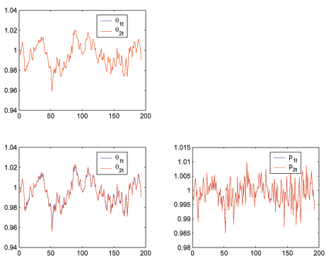
While market tightness, and hence relative market tightness, is of course not a price in the typically-understood sense, it is a market-based signal that coordinates the activity of both firms and households. Recall that expressions (11) and (12) showed that relative market tightness governs the composition of search and advertising activity across cash search and credit search markets. To the extent that unanticipated inflation would cause an inefficient composition of search activity, unanticipated inflation is undesirable. At its core, this type of mechanism is quite similar to that articulated by any basic sticky-price model: with sticky prices, the typical intuition behind the optimality of low variability of inflation is that it supports an efficient composition of output.¹² It is this tight analogy that motivates us to refer to $\theta_{1t}/\theta_{2t}$ as a relative price.

Figure 2:  Log deviations of restricted-Ramsey-optimal tightness and prices in cash and credit sectors with restriction that $R_{t} = \bar{R}$ $\forall t$.

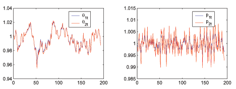
For comparison, we also construct an alternative, restricted-Ramsey, equilibrium in which money growth and hence inflation are more volatile than under the Ramsey policy. The alternative policy we consider is one in which the nominal interest rate is always constant at its steady-state level, implying that all shifts in monetary policy must be accommodated by (larger) variations in the money growth rate, which would tend to be associated with larger state-contingent variations in inflation.¹³ For the same set of shocks as in Figure 1, Figure 2 displays how tightness and prices move under this restricted-Ramsey policy. The correlation between $\theta _{1t}$ and $\theta_{2t}$ is 0.95 under this arbitrary policy; while still high in an absolute sense, it is clearly lower than under the fully-optimal policy. The standard deviation of the inflation rate under this alternative dynamic policy is 1.29, double that under the true Ramsey policy. Thus, the key idea we want to point out with this arbitrary policy is that higher variability of unanticipated inflation is associated with lower correlation between the market tightness variables $\theta_{1t}$ and $\theta_{2t}$, further suggesting that pursuing a policy of low inflation volatility is optimal.

Figure 3:  Optimal inflation volatility (standard deviation in annualized percentage points) as a function of $\vartheta$.

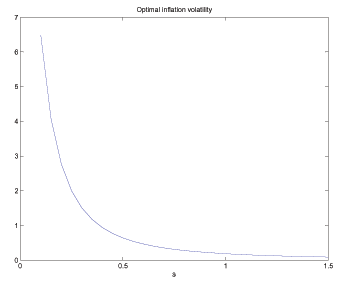
Figure 3 demonstrates a different dimension of our results, illustrating the quantitative power of the search friction in shaping optimal policy. In Figure 3, we plot the standard deviation of the Ramsey inflation rate as a function of $\vartheta$, which, recall from the specification of household preferences in (1), governs how valuable search goods are to the household; all other parameter values are held constant at their benchmark levels. In the absence of direct evidence, recall that we set as our baseline $\vartheta=1$. In the limit, setting $\vartheta= 0$ collapses our model to a standard CCK model.

Figure 3 clearly shows that as we move our environment close to that of CCK (by lowering $\vartheta$), their benchmark inflation volatility result re-emerges. As $\vartheta$ rises from very low values, optimal inflation volatility falls quickly, approaching a basic sticky-price model's prediction of near-zero inflation volatility for sufficiently-large $\vartheta$. We encountered numerical difficulty in solving for very small and very large values of $\vartheta$, hence we limit the results in Figure 3 to $\vartheta\in[0.1, 1.5]$, but the main message seems clear: as the importance of goods obtained in long-term relationships grows (governed by increasing $\vartheta$), stabilizing inflation becomes an ever-more important goal of policy.

4.3.2  Ramsey Allocations

In terms of the dynamics of allocations, the first row of the lower panel of Table 2 shows that the volatility of GDP, at about 1.8 percent, is in line with the empirical evidence for the U.S. economy presented in King and Rebelo (1999) and with many DSGE models, so there is nothing unusual about the macrodynamics of our model. Table 2 also shows that the dynamics of $a_{1}$ follow very closely the dynamics of $a_{2}$, the dynamics of $s_{1}$ follow very closely the dynamics of $s_{2}$, the dynamics of $N_{1}$ follow very closely the dynamics of $N_{2}$, and the dynamics of $\theta_{1}$ follow very closely the dynamics of $\theta_{2}$. These results all seem natural given the symmetry of our calibration across the cash search and credit search sectors. Also, the correlation between $s_{1t}$ and $s_{2t}$ is virtually unity, as is that between $a_{1t}$ and $a_{2t}$, confirming the no-arbitrage relationships across the cash and credit sectors. We leave our discussion of Ramsey allocations at that, but Table 2 presents some other moments calculated from our simulations.

5  Conclusion

The idea that unanticipated inflation is undesirable because it distorts relative prices is a well-established one. It is an idea articulated in basic undergraduate textbooks, and it is embedded in a very simple way - through the assumption of sticky prices -- in the modern New Keynesian models that provide the basis for much of the model-based discussions of monetary policy issues. We show that deep-rooted frictions underlying goods-market trades lead to much the same effect. We adapted a standard cash/credit model, one that has been a workhorse in Ramsey studies of monetary policy, to include fundamental transactions frictions in what we view is at least one very natural way. With this simple extension, we show that achieving inflation stability is an important objective of policy. The importance of inflation stability stems from a type of relative-price distortion that arises absent such a policy; this relative-price distortion governs the composition of search activity across markets. even though there are no nominal rigidities of any sort. Our results thus complement the standard view that sticky prices must be at the core of any practical DSGE model of monetary policy.

A natural extension to pursue would be to consider alternative pricing arrangements. We employed Nash bargaining in our model of goods markets, as do Arseneau and Chugh (2007b) and Hall (2007), because it is well-understood in search and matching frameworks. For goods market trades, allowing for price-posting by firms along with directed search by households -- a combination of features referred to in the search literature as competitive search equilibrium (see Rogerson, Shimer, and Wright (2005)) -- seems very natural. To our knowledge, no DSGE search-based models (we have in mind here the recent vintages of DSGE labor-search models) have yet incorporated competitive search equilibrium. In a competitive search equilibrium, the relationship between prices and market tightness is different than in Nash bargaining. It may be important to know how and to what extent our results carry over to such an environment.

As we mentioned at the outset, our work builds on the theme begun in Arseneau and Chugh (2007a) and Aruoba and Chugh (2006) of studying optimal policy in environments with deep-rooted frictions in key markets. With the lessons learned by studying optimal policy in the face of fundamental trading frictions in labor markets (Arseneau and Chugh (2007b)), in one type of financial market (money markets -- Aruoba and Chugh (2006)), and now here in product markets, an obvious interesting next step would be to characterize optimal policy in the presence of more than one of these frictions. Such a project would move this emerging second-generation of Ramsey-based optimal policy models even closer to the medium- and large-scale quantitative models favored by central banks as one input in their policy-making process. Some of the insights to be learned may be quite similar to those from existing models; some of the lessons are likely to be quite different.

Appendix A:  Household Problem

The representative household's problem in the baseline model is to choose state-contingent rules for $l_{t}$, $x_{1t}$, $x_{2t}$, $M_{t}$, $B_{t}$, $N^{h}_{1t+1}$, $N^{h}_{2t+1}$, $s_{1t}$, and $s_{2t}$ to maximize

$$E_{0} \sum_{t=0}^{\infty} \beta^{t} \left[ u(x_{1t}, x_{2t}) + \vartheta v\left( \int_{0}^{N^{h}_{1t}} c_{i1t} di, \int_{0} ^{N^{h}_{2t}} c_{i2t} di \right) + g(1-l_{t}-s_{t}-N^{h}_{t}) \right]$$ (39)

subject to the sequence of flow budget constraints

$$\lefteqn{M_{t} - M_{t-1} + B_{t} - R_{t-1} B_{t-1} = }$$ (40)

$$(1-\tau^{l}_{t-1})W_{t-1} l_{t-1} - P_{t-1} x_{1t-1} - P_{t-1} x_{2t-1} - \int_{0}^{N^{h}_{1t-1}} P_{i1t-1} c_{i1t-1} di - \int_{0}^{N^{h}_{2t-1}} P_{i2t-1} c_{i2t-1} di + P_{t-1} d_{t-1},$$

the sequence of cash-in-advance constraints

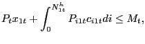
$$P_{t} x_{1t} + \int_{0}^{N^{h}_{1t}} P_{i1t} c_{i1t} di \leq M_{t},$$ (41)

perceived laws of motion for the number of active cash relationships,

$$N^{h}_{1t+1} = (1-\rho^{x}) ( N^{h}_{1t} + s_{1t} k^{h}(\theta_{1t}) )$$ (42)

and credit relationships

$$N^{h}_{2t+1} = (1-\rho^{x}) ( N^{h}_{2t} + s_{2t} k^{h}(\theta_{2t}) ),$$ (43)

as well as the identities

$$N^{h}_{t} = N^{h}_{1t} + N^{h}_{2t}$$ (44)

and

$$s_{t} = s_{1t} + s_{2t}.$$ (45)

Substitute the identities (44) and (45) directly into the utility function. Associate the sequence of multipliers $\phi_{t} / P_{t-1}$, $\lambda_{t} / P_{t}$, $\mu ^{h}_{1t}$, and $\mu^{h}_{2t}$ to the remaining constraints, respectively. The first-order conditions with respect to $l_{t}$, $x_{1t}$, $x_{2t}$, $M_{t}$, $B_{t}$, $N^{h}_{1t+1}$, $N^{h}_{2t+1}$, $s_{1t}$, and $s_{2t}$ are, respectively,

$$-g^{\prime}_{t} + (1-\tau^{l}_{t}) w_{t} \beta E_{t} \phi_{t+1} = 0,$$ (46)

$$u_{1t} - \lambda_{t} - \beta E_{t} \phi_{t+1} = 0,$$ (47)

$$u_{2t} - \beta E_{t} \phi_{t+1} = 0,$$ (48)

$$-\frac{\phi_{t}}{P_{t-1}} + \frac{\lambda_{t}}{P_{t}} + \beta E_{t} \left( \frac{\phi_{t+1}}{P_{t}}\right) = 0,$$ (49)

$$-\frac{\phi_{t}}{P_{t-1}} + \beta R_{t} E_{t}\left( \frac{\phi_{t+1}}{P_{t}}\right) = 0,$$ (50)

$$\beta E_{t} \left\{ \vartheta v_{1t+1} c_{1t+1} \right\} - \beta E_{t} g^{\prime}_{t+1} - \mu^{h}_{1t} + \beta(1-\rho^{x}) E_{t} \mu^{h}_{1t+1} - \beta E_{t} \left\{ \lambda_{t+1} \frac{P_{1t+1} }{P_{t+1}} c_{1t+1} \right\} - \beta E_{t} \left\{ \beta\phi_{t+2} \frac{P_{1t+1}}{P_{t+1}} c_{1t+1} \right\} = 0,$$ (51)

$$\beta E_{t} \left\{ \vartheta v_{2t+1} c_{2t+1} \right\} - \beta E_{t} g^{\prime}_{t+1} - \mu^{h}_{2t} + \beta(1-\rho^{x}) E_{t} \mu^{h}_{2t+1} - \beta E_{t} \left\{ \beta\phi_{t+2} \frac{P_{2t+1} }{P_{t+1}} c_{2t+1} \right\} = 0,$$ (52)

$$-g^{\prime}_{t} + (1-\rho^{x}) \mu^{h}_{1t} k^{h}(\theta_{1t}) = 0,$$ (53)

$$-g^{\prime}_{t} + (1-\rho^{x}) \mu^{h}_{2t} k^{h}(\theta_{2t}) = 0.$$ (54)

The first-order conditions (46) through (50) are completely standard in cash/credit models; they imply a standard consumption-leisure optimality condition

$$\frac{g^{\prime}(1-l_{t}-s_{t}-N^{h}_{t} )}{u_{2t}} = (1-\tau^{l}_{t}) w_{t},$$ (55)

a (Walrasian) cash-good/credit-good optimality condition

$$\frac{u_{1t}}{u_{2t}} = R_{t},$$ (56)

and a pricing formula for a one-period nominally risk-free bond

$$1 = R_{t} E_{t} \left[ \frac{\beta u_{1t+1}}{u_{1t}} \frac{1}{\pi_{t+1}} \right] ,$$ (57)

where $\pi_{t} \equiv P_{t} / P_{t-1}$ is the gross inflation rate between periods $t-1$ and $t$.

Regarding the search markets, the first-order conditions (51) and (53) yield an optimal shopping condition for cash goods,

$$\frac{g^{\prime}_{t}}{k^{h}(\theta_{1t})} = \beta(1-\rho^{x}) E_{t} \left\{ c_{1t+1} \left[ \vartheta v_{1t+1} - p_{1t+1} u_{1t+1} \right] - g^{\prime}_{t+1} + \frac{g^{\prime}_{t+1}}{k^{h} (\theta_{1t+1})} \right\} ,$$ (58)

which is expression (9) in the text; and the first-order conditions (52) and (54) yield an optimal shopping condition for credit goods,

$$\frac{g^{\prime}_{t}}{k^{h}(\theta_{2t})} = \beta(1-\rho^{x}) E_{t} \left\{ c_{2t+1} \left[ \vartheta v_{2t+1} - p_{2t+1} u_{2t+1} \right] - g^{\prime}_{t+1} + \frac{g^{\prime}_{t+1}}{k^{h} (\theta_{2t+1})} \right\} ,$$ (59)

which is expression (10) in the text.

Appendix B:  Nash Bargaining

The marginal value to the household of a family member who is actively engaged in a cash relationship with a firm (in nominal terms):

$$\mathbf{M^{1}_{t}} = \frac{P_{t} \tilde{v}^{1}(c_{i1t})}{\beta E_{t} \phi_{t+1} + \lambda_{t}} - \frac{P_{t} g^{\prime}(1-l_{t}-s_{t}-N_{t})}{\beta E_{t} \phi_{t+1} + \lambda_{t}} - P_{i1t} c_{i1t} + E_{t} \left[ \left( \Xi_{t+1\vert t}\frac{P_{t}}{P_{t+1}} \right) ( (1-\rho^{x}) \mathbf{M^{1}_{t+1}} + \rho^{x} \mathbf{S^{1}_{t+1}} ) \right] .$$ (60)

The marginal value to the household of a family member who is actively engaged in a credit relationship with a firm (in nominal terms):

$$\mathbf{M^{2}_{t}} = \frac{P_{t} \tilde{v}^{2}(c_{i2t})}{\beta E_{t} \phi_{t+1}} - \frac{P_{t} g^{\prime}(1-l_{t}-s_{t}-N_{t})}{\beta E_{t} \phi_{t+1}} - P_{i2t} c_{i2t} + E_{t} \left[ \left( \Xi_{t+1\vert t}\frac{P_{t} }{P_{t+1}} \right) ( (1-\rho^{x}) \mathbf{M^{2}_{t+1}} + \rho^{x} \mathbf{S^{1}_{t+1}} ) \right] .$$ (61)

The function $\tilde{v}^{1}(.)$ is the marginal utility to the household of obtaining cash consumption from the $i$-th match, and $\tilde{v}^{2}(.)$ is the marginal utility to the household of obtaining credit consumption from the $i$-th match. Hence, $\tilde{v}^{i}(.) \equiv v_{it}(.)$, $i = 1,2$. Captured in these Bellman equations is the assumption that if a given customer relationship survives separation, it continues to be a cash (credit) relationship if it was previously a cash (credit) relationship. Note that the discount used for $\mathbf{M^{1}_{t}}$ is different from the discount used for $\mathbf{M^{2}_{t}}$. Because of our assumption that a cash relationship is always a cash relationship and a credit relationship is always a credit relationship, the nominal interest rate needs to be taken account of in defining these two asset values. Because in equilibrium, $\beta E_{t} \phi_{t+1} = u_{2t}$, $\beta E_{t} \phi_{t+1} + \lambda_{t} = u_{1t}$, and $u_{1t}/u_{2t} = R_{t}$, defining the asset values this way does this.

For tractability and in line with our assumption that cash (credit) relationships are always cash (credit) relationships, we assume that a cash (credit) relationship can result only from purposeful search in the cash (credit) market. An extension one may want to later pursue is to allow crossover from search in one market into active relationships in the other market. The marginal value to the household of an individual searching for a cash relationship and an individual searching for a credit relationship thus are, respectively,

$$\mathbf{S^{1}_{t}} = -\frac{P_{t} g^{\prime}(1-l_{t}-s_{t}-N_{t})}{\beta E_{t} \phi_{t+1} + \lambda_{t}} + E_{t} \left[ \left( \Xi_{t+1\vert t} \frac{P_{t} }{P_{t+1}}\right) \left( \theta_{1t} k^{f}(\theta_{1t}) (1-\rho^{x}) \mathbf{M^{1}_{t+1}} + (1-\theta_{1t}k^{f}(\theta_{1t})(1-\rho^{x} ))\mathbf{S^{1}_{t+1}} \right) \right]$$ (62)

and

$$\mathbf{S^{2}_{t}} = -\frac{P_{t} g^{\prime}(1-l_{t}-s_{t}-N_{t})}{\beta E_{t} \phi_{t+1}} + E_{t} \left[ \left( \Xi_{t+1\vert t} \frac{P_{t}}{P_{t+1}}\right) \left( \theta_{2t} k^{f}(\theta_{2t}) (1-\rho^{x}) \mathbf{M^{2}_{t+1}} + (1-\theta_{2t}k^{f}(\theta_{2t})(1-\rho^{x}))\mathbf{S^{2}_{t+1}} \right) \right] .$$ (63)

By the properties of the Cobb-Douglas matching function, $k^{h}(\theta_{it}) = \theta_{it} k^{f}(\theta_{it})$. Notice that in these formulations of $\mathbf{S^{1}_{t}}$ and $\mathbf{S^{2}_{t}}$, we make the assumption that if an individual is not successful in forming a lasting customer relationship, he is assigned back to search in the next period. In principle, a given atomistic individual unsuccessful in forming a customer relationship could be assigned by the household to labor or leisure in the next period, as well. Our specification is without loss of generality, however, because the household in every period optimally allocates its members between cash-search and credit-search. That is, as we allude to in the text, there is essentially a "no-arbitrage" condition between cash search and credit search a the household level, making the precise identities of those assigned to search in one sector versus the other irrelevant. Thus, without loss of generality, we can suppose that an individual who continues to search from one period to the next does so in the same sector.

The values to a firm of an existing cash customer and an existing credit customer are, respectively,

$$\mathbf{A^{1}_{t}} = P_{i1t} c_{i1t} - mc_{t} c_{i1t} + E_{t} \left[ \left( \Xi_{t+1\vert t} \frac{P_{t}}{P_{t+1}}\right) (1-\rho^{x}) \mathbf{A^{1}_{t+1}} \right]$$ (64)

and

$$\mathbf{A^{2}_{t}} = P_{i2t} c_{i2t} - mc_{t} c_{i2t} + E_{t} \left[ \left( \Xi_{t+1\vert t} \frac{P_{t}}{P_{t+1}}\right) (1-\rho^{x}) \mathbf{A^{2}_{t+1}} \right] .$$ (65)

Bargaining occurs every period between a given customer and the firm with which he is engaged in a relationship. For $i=1,2$, the firm and customer maximize the Nash product

$$(\mathbf{M^{i}_{t}} - \mathbf{S^{i}_{t}})^{\eta}\mathbf{A^{i}_{t}}^{1-\eta},$$ (66)

where $\eta\in(0,1)$ is the fixed weight given to the customer's (equivalently, the household's) surplus and identical across cash and credit relationships. Make the following changes of variables: divide $\mathbf{M^{i} _{t}}$, $\mathbf{S^{i}_{t}}$, and $\mathbf{A^{i}_{t}}$ by $P_{t}$, define $p_{it} = P_{it}/P_{t}$ as the relative price of a search good, and re-interpret the asset values to be real, rather than nominal, asset values. With these changes, the first-order condition of the Nash product with respect to $p_{it}$ is

$$\eta(\mathbf{M^{i}_{t}}-\mathbf{S^{i}_{t}})^{\eta-1} \left( \frac {\partial\mathbf{M^{i}_{t}}}{\partial p_{it}} - \frac{\partial\mathbf{S^{i} _{t}}}{\partial p_{it}}\right) \mathbf{A^{i}_{t}}^{1-\eta} + (1-\eta) (\mathbf{M^{i}_{t}}-\mathbf{S^{i}_{t}})^{\eta} \mathbf{A^{i}_{t}}^{-\eta} \frac{\partial\mathbf{A^{i}_{t}}}{\partial p_{it}} = 0,$$ (67)

which can be condensed as usual to

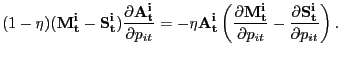
$$(1-\eta) (\mathbf{M^{i}_{t}} - \mathbf{S^{i}_{t}}) \frac{\partial \mathbf{A^{i}_{t}}}{\partial p_{it}} = -\eta\mathbf{A^{i}_{t}} \left( \frac{\partial\mathbf{M^{i}_{t}}}{\partial p_{it}} - \frac{\partial \mathbf{S^{i}_{t}}}{\partial p_{it}} \right) .$$ (68)

Using the value functions above and going through several tedious steps of algebra, all of which are identical to those in Arseneau and Chugh (2007b), we have

$$p_{1t} c_{1,t} = (1-\eta) \left( \frac{\tilde{v}^{1}(c_{1t})}{u_{1t}} \right) + \eta(mc_{t} c_{1,t} - \gamma\theta_{1t})$$ (69)

and

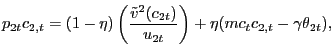
$$p_{2t} c_{2,t} = (1-\eta) \left( \frac{\tilde{v}^{2}(c_{2t})}{u_{2t}} \right) + \eta(mc_{t} c_{2,t} - \gamma\theta_{2t}),$$ (70)

which are expressions (22) and (23) in the text.

Appendix C  Private-Sector Equilibrium

Here, we collect the conditions characterizing a symmetric search equilibrium defined in Section 2.8. They are:

• Resource constraint:

  $$x_{1t} + x_{2t} + N_{1t} c_{1t} + N_{2t} c_{2t} + g_{t} + \gamma(a_{1t} + a_{2t}) = z_{t} l_{t}$$ (71)

  
  
• The standard (Walrasian) cash-credit optimality condition:

  $$\frac{u_{1t}}{u_{2t}} = R_{t}$$ (72)

  
  
• The standard consumption-leisure optimality condition:

  $$\frac{g^{\prime}_{t}}{u_{2t}} = (1-\tau^{l}_{t}) w_{t}$$ (73)

  
  
• The standard bond Euler equation (pricing formula for a one-period nominally risk-free bond):

  $$1 = R_{t} E_{t} \left[ \frac{\beta u_{1t+1}}{u_{1t}} \frac{1}{\pi_{t+1}} \right]$$ (74)

  
  
• The (two different) shopping conditions for cash relationships and credit relationships:

  $$\frac{g^{\prime}_{t}}{k^{h}(\theta_{t})} = (1-\rho^{x}) E_{t} \left\{ c_{1t+1} \left[ \vartheta v_{1t+1} - p_{1t+1} u_{1t+1} \right] - g^{\prime}_{t+1} + \frac{g^{\prime}_{t+1}}{k^{h}(\theta_{t+1})} \right\}$$ (75)

  
  

  $$\frac{g^{\prime}_{t}}{k^{h}(\theta_{t})} = (1-\rho^{x}) E_{t} \left\{ c_{2t+1} \left[ \vartheta v_{2t+1} - p_{2t+1} u_{2t+1} \right] - g^{\prime }_{t+1} + \frac{g^{\prime}_{t+1}}{k^{h}(\theta_{t+1})} \right\}$$ (76)

  
  
• The (two different) advertising conditions for cash relationships and credit relationships:

  $$\frac{\gamma}{k^{f}(\theta_{t})} = \beta(1-\rho^{x}) E_{t} \left\{ \Xi_{t+1\vert t} \left( p_{1t+1} c_{1t+1} - mc_{t+1} c_{1t+1} + \frac{ \gamma }{k^{f}(\theta_{t+1})} \right) \right\}$$ (77)

  
  

  $$\frac{\gamma}{k^{f}(\theta_{t})} = \beta(1-\rho^{x}) E_{t} \left\{ \Xi_{t+1\vert t} \left( p_{2t+1} c_{2t+1} - mc_{t+1} c_{2t+1} + \frac{ \gamma }{k^{f}(\theta_{t+1})} \right) \right\}$$ (78)

  
  
• Nash-pricing equations to pin down $p_{1t}$ and $p_{2t}$:

  $$p_{1t} c_{1,t} = (1-\eta) \left( \frac{\tilde{v}^{1}(c_{1t})}{u_{1t}} \right) + \eta(mc_{t} c_{1,t} - \gamma\theta_{1t})$$ (79)

  
  

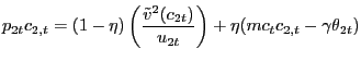
  $$p_{2t} c_{2,t} = (1-\eta) \left( \frac{\tilde{v}^{2}(c_{2t})}{u_{2t}} \right) + \eta(mc_{t} c_{2,t} - \gamma\theta_{2t})$$ (80)

  
  
• Aggregate laws of motion for active cash and credit customer relationships:

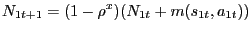
  $$N_{1t+1} = (1-\rho^{x}) (N_{1t} + m(s_{1t}, a_{1t}))$$ (81)

  
  

  $$N_{2t+1} = (1-\rho^{x}) (N_{2t} + m(s_{2t}, a_{2t}))$$ (82)

  
  
• Condition describing nominal price inflation:

  $$\pi_{t} \left[ \frac{x_{1t} + p_{1t} N_{1t} c_{1t}}{x_{1t-1} + p_{1t-1} N_{1t-1} c_{1t-1}} \right] = \mu_{t},$$ (83)

  
  
• Efficient labor market:

  $$w_{t} = z_{t}$$ (84)

  
  

Appendix D  Derivation of PVIC

The derivation of the Ramsey present-value implementability constraint (PVIC) proceeds quite similarly to derivations in standard flexible-price Ramsey models. Unlike standard flexible-price Ramsey models, and as we mentioned in Section 3, the PVIC in our model does not encode all of the equilibrium conditions of the economy; in particular, it does not encode the conditions describing search and pricing activity in the cash and credit search markets.

To derive the PVIC, start as usual with the household flow budget constraint in symmetric equilibrium. Diving each term through by $P_{t-1}$, multiplying each term by $\beta^{t} \phi_{t}$, and summing from $t=0$ to infinity gives

$$\lefteqn{ \sum_{t=0}^{\infty} \beta^{t} \phi_{t} x_{1t-1} + \sum_{t=0} ^{\infty} \beta^{t} \phi_{t} x_{2t-1} + \sum_{t=0}^{\infty} \beta^{t} \phi_{t} p_{1t-1} N_{1t-1} c_{1t-1} + \sum_{t=0}^{\infty} \beta^{t} \phi_{t} p_{2t-1} N_{2t-1} c_{2t-1} + \sum_{t=0}^{\infty} \beta^{t} \phi_{t} \frac{M_{t} }{P_{t-1}} }$$

$$+ \sum_{t=0}^{\infty} \beta^{t} \phi_{t} \frac{B_{t}}{P_{t-1}} = \sum_{t=0}^{\infty} \beta^{t} \phi_{t} (1-\tau^{l}_{t-1}) w_{t-1} l_{t-1} + \sum_{t=0}^{\infty} \beta^{t} \phi_{t} \frac{M_{t-1}}{P_{t-1}} + \sum _{t=0}^{\infty} \beta^{t} \phi_{t} R_{t-1} \frac{B_{t-1}}{P_{t-1}} + \sum_{t=0}^{\infty} \beta^{t} \phi_{t} d_{t-1}.$$

Use the household first-order condition (49) to substitute into the last term on the first line and use the household first-order condition (50) to substitute into the first term on second line; this yields

$$\lefteqn{ \sum_{t=0}^{\infty} \beta^{t} \phi_{t} x_{1t-1} + \sum_{t=0} ^{\infty} \beta^{t} \phi_{t} x_{2t-1} + \sum_{t=0}^{\infty} \beta^{t} \phi_{t} p_{1t-1} N_{1t-1} c_{1t-1} + \sum_{t=0}^{\infty} \beta^{t} \phi_{t} p_{2t-1} N_{2t-1} c_{2t-1} }$$

$$+ \sum_{t=0}^{\infty} \beta^{t} \lambda_{t} \frac{M_{t}}{P_{t}} + \sum_{t=0}^{\infty} \beta^{t} \beta\phi_{t+1} \frac{M_{t}}{P_{t}} + \sum _{t=0}^{\infty} \beta^{t} \beta\phi_{t+1} R_{t} \frac{B_{t}}{P_{t}}$$

$$= \sum_{t=0}^{\infty} \beta^{t} \phi_{t} (1-\tau^{l}_{t-1}) w_{t-1} l_{t-1} + \sum_{t=0}^{\infty} \beta^{t} \phi_{t} \frac{M_{t-1}}{P_{t-1}} + \sum_{t=0}^{\infty} \beta^{t} \phi_{t} R_{t-1} \frac{B_{t-1}}{P_{t-1}} + \sum_{t=0}^{\infty} \beta^{t} \phi_{t} d_{t-1}.$$

Canceling like summations, pulling out the $t=0$ terms from several summations, and adjusting indices of summation yields

$$\lefteqn{ \sum_{t=0}^{\infty}\beta^{t} \beta\phi_{t+1} x_{1t} + \sum _{t=0}^{\infty}\beta^{t} \beta\phi_{t+1} x_{2t} + \sum_{t=0}^{\infty}\beta^{t} \beta\phi_{t+1} p_{1t}N_{1t}c_{1t} + \sum_{t=0}^{\infty}\beta^{t} \beta \phi_{t+1} p_{2t}N_{2t}c_{2t} + \sum_{t=0}^{\infty}\beta^{t} \lambda_{t} \frac{M_{t}}{P_{t}} }$$

$$= \sum_{t=0}^{\infty} \beta^{t} \beta\phi_{t+1} (1-\tau^{l}_{t})w_{t} l_{t} + \sum_{t=0}^{\infty} \beta^{t} \beta\phi_{t+1} d_{t}$$

$$+ \phi_{0} \left[ \frac{M_{-1} + R_{-1} B_{-1}}{P_{-1}} + (1-\tau^{l} _{-1}) w_{-1} l_{-1} - x_{1,-1} - x_{2,-1} - p_{1,-1}N_{1,-1}c_{1,-1} - p_{2,-1}N_{2,-1}c_{2,-1} + d_{-1} \right] .$$

Define

$${\small A_{0} = \phi_{0} \left[ \frac{M_{-1} + R_{-1} B_{-1}}{P_{-1}}\right] + \phi_{0} \left[ (1-\tau^{l}_{-1}) w_{-1} l_{-1} - mc_{-1} N_{1,-1} c_{1,-1} - mc_{-1} N_{2,-1} c_{2,-1} - \gamma(a_{1,-1} + a_{2,-1}) - x_{1,-1} - x_{2,-1} \right] .}$$ (85)

With this definition, substitute into the previous expression the symmetric equilibrium expression for real dividend payments of the firm, $d_{t} = (p_{1t} - mc_{t}) N_{1t} c_{1t} + (p_{2t} - mc_{t})N_{2t} c_{2t} - \gamma(a_{1t} + a_{2t})$ , which gives

$$\lefteqn{ \sum_{t=0}^{\infty}\beta^{t} \beta\phi_{t+1} x_{1t} + \sum _{t=0}^{\infty}\beta^{t} \beta\phi_{t+1} x_{2t} + \sum_{t=0}^{\infty}\beta^{t} \beta\phi_{t+1} p_{1t}N_{1t}c_{1t} + \sum_{t=0}^{\infty}\beta^{t} \beta \phi_{t+1} p_{2t}N_{2t}c_{2t} + \sum_{t=0}^{\infty}\beta^{t} \lambda_{t} \frac{M_{t}}{P_{t}} }$$

$$= \sum_{t=0}^{\infty} \beta^{t} \beta\phi_{t+1} (1-\tau^{l}_{t})w_{t} l_{t} + \sum_{t=0}^{\infty} \beta^{t} \beta\phi_{t+1} (p_{1t}-mc_{t}) N_{1t}c_{1t}$$

$$+ \sum_{t=0}^{\infty} \beta^{t} \beta\phi_{t+1} (p_{2t}-mc_{t} )N_{2t}c_{2t} - \sum_{t=0}^{\infty} \beta^{t} \beta\phi_{t+1} \gamma (a_{1t}+a_{2t}) + A_{0}.$$

Using the cash-in-advance constraint holding with equality, $\frac{M_{t} }{P_{t}} = x_{1t} + p_{1t} N_{1t} c_{1t}$, to substitute out the term involving $\frac{M_{t}}{P_{t}}$ yields

$$\lefteqn{ \sum_{t=0}^{\infty}\beta^{t} \beta\phi_{t+1} x_{1t} + \sum _{t=0}^{\infty} \beta^{t} \lambda_{t} x_{1t} + \sum_{t=0}^{\infty}\beta^{t} \beta\phi_{t+1} x_{2t} + \sum_{t=0}^{\infty}\beta^{t} \beta\phi_{t+1} p_{1t}N_{1t}c_{1t} + \sum_{t=0}^{\infty}\beta^{t} \lambda_{t} p_{1t} N_{1t}c_{1t} }$$

$$+ \sum_{t=0}^{\infty}\beta^{t} \beta\phi_{t+1} p_{2t}N_{2t}c_{2t} = \sum_{t=0}^{\infty} \beta^{t} \beta\phi_{t+1} (1-\tau^{l}_{t})w_{t} l_{t} + \sum_{t=0}^{\infty} \beta^{t} \beta\phi_{t+1} (p_{1t}-mc_{t}) N_{1t}c_{1t}$$

$$+ \sum_{t=0}^{\infty} \beta^{t} \beta\phi_{t+1} (p_{2t}-mc_{t} )N_{2t}c_{2t} - \sum_{t=0}^{\infty} \beta^{t} \beta\phi_{t+1} \gamma (a_{1t}+a_{2t}) + A_{0}.$$

Next, using the household first-order conditions $\beta E_{t} \phi_{t+1} = u_{2t}$ and $\beta E_{t} \phi_{t+1} + \lambda_{t} = u_{1t}$, we have

$$\lefteqn{ \sum_{t=0}^{\infty}\beta^{t} u_{1t} x_{1t} + \sum_{t=0}^{\infty }\beta^{t} u_{2t}x_{2t} + \sum_{t=0}^{\infty}\beta^{t} u_{1t} p_{1t} N_{1t}c_{1t} + \sum_{t=0}^{\infty}\beta^{t} u_{2t}p_{2t}N_{2t}c_{2t} }$$

$$= \sum_{t=0}^{\infty} \beta^{t} u_{2t} (1-\tau^{l}_{t})w_{t} l_{t} + \sum_{t=0}^{\infty} \beta^{t} u_{2t} (p_{1t}-mc_{t}) N_{1t}c_{1t} + \sum _{t=0}^{\infty} \beta^{t} u_{2t} (p_{2t}-mc_{t})N_{2t}c_{2t} - \sum _{t=0}^{\infty} \beta^{t} u_{2t} \gamma(a_{1t}+a_{2t}) + A_{0}.$$

Finally, use the consumption-leisure optimality condition to substitute $g^{\prime}_{t} = u_{2t}(1-\tau^{l}_{t})w_{t}$ and rearrange terms to arrive at the PVIC,

$$E_{0} \sum_{t=0}^{\infty} \beta^{t} \left[ u_{1t} x_{1t} + u_{2t} x_{2t} - g^{\prime}_{t} l_{t} + (u_{1t} - u_{2t}) p_{1t} N_{1t} c_{1t} + u_{2t} mc_{t} N_{1t} c_{1t} + u_{2t} mc_{t} N_{2t} c_{2t} + u_{2t} \gamma(a_{1t} + a_{2t}) \right] = A_{0},$$ (86)

which is expression (31) in the text.

When we allow for the profit tax and search taxes, the household flow budget constraint is modified to

$$\lefteqn{M_{t} - M_{t-1} + B_{t} - R_{t-1} B_{t-1} = \tau^{s_{1}}_{t-1} s_{1t-1} + \tau^{s_{2}}_{t-1} s_{2t-1} }$$ (87)

$$+ (1-\tau^{l}_{t-1})W_{t-1} l_{t-1} - P_{t-1} x_{1t-1} - P_{t-1} x_{2t-1}$$ (88)

$$- \int_{0}^{N^{h}_{1t-1}} P_{i1t-1} c_{i1t-1} di - \int_{0}^{N^{h}_{2t-1}} P_{i2t-1} c_{i2t-1} di + (1-\tau^{pr}_{t-1}) P_{t-1} d_{t-1}.$$

Proceeding just as before, except refraining from combining the equilibrium expression for $d_{t}$ as we did above, we have that the PVIC is

$$\lefteqn{ \sum_{t=0}^{\infty} \beta^{t} \left[ u_{1t} x_{1t} + u_{2t} x_{2t} + u_{1t} p_{1t} N_{1t} c_{1t} + u_{2t} p_{2t} N_{2t} c_{2t} - g'_{t} l_{t} - u_{2t} \tau^{s_{1}} s_{1t} - u_{2t} \tau^{s_{2}} s_{2t} \right] }$$ (89)

$$- \sum_{t=0}^{\infty}\beta^{t} \left[ (1-\tau^{pr}_{t}) \left( u_{2t}(p_{1t}-mc_{t})N_{1t}c_{1t} + u_{2t}(p_{2t}-mc_{t})N_{2t}c_{2t} - u_{2t} \gamma(a_{1t} + a_{2t}) \right) \right] = A_{0}.$$ (90)

Setting $\tau^{s_{1}}_{t} = \tau^{s_{2}}_{t} = \tau^{pr}_{t} = 0$ $\forall t$ and combining several terms collapses this modified PVIC back to expression (31).

Appendix E  Effects of Exogenous Policy on Search Behavior

In the standard CCK model, a deviation from the Friedman Rule is costly because it distorts the marginal rate of substitution between cash and credit goods. Implementing the Friedman Rule requires the Ramsey planner to raise the funds to finance the attendant deflation via the labor tax.¹⁴ In the standard CCK model, financing a deflation with proportional labor income taxation does not generate any other distortions that undermine the optimality of the Friedman Rule. This conclusion does not carry over to our model for two reasons. To elucidate them, it is helpful to first consider how completely exogenous tax rates and nominal interest rates affect search behavior in our environment, channels of course not present in a standard model of goods markets.

First, due to the presence of search frictions and the fact that search and leisure are both alternatives to labor as uses of a household's time, the labor income tax distorts not only labor supply but also household shopping behavior. This is true even though ostensibly the Hosios parameterization for search efficiency is in place. Just as in the standard CCK model, all else equal, a higher labor tax rate causes households to substitute out of labor ($l$) and into leisure $(1-l-s_{1}-s_{2}-N_{1}-N_{2} )$. However, in our environment, the resulting decline in the marginal utility of leisure, $g^{\prime}(1-l-s_{1}-s_{2}-N_{1}-N_{2})$, means that the cost of engaging in additional search activity falls as well, inducing households to spend more time searching for goods.¹⁵ That is, $s_{1}$ and $s_{2}$ both rise as $\tau^{l}$ rises. To isolate this effect, we plot in the top row of Figure 4 the long-run responses of $s_{1}$ and $s_{2}$ to exogenous changes in the labor tax rate, holding monetary policy fixed at the Friedman Rule.¹⁶ The resulting slackness in product markets (by which we mean a fall in $\theta_{1}$ and $\theta_{2}$) induces firms to reduce advertising expenditures because a given level of advertising now more readily yields new customers.¹⁷ On net, the decline in advertising expenditures dominates, causing the number of active customer relationships ($N_{1}$ and $N_{2}$) to fall. Thus, because the labor tax distorts household labor supply, it also directly distorts shopping behavior and indirectly distorts advertising behavior. These latter effects, absent in a standard CCK model, make the welfare consequences of running the Friedman deflation financed via a labor tax quite different in our environment.

Figure 4:  Steady-state household search behavior under exogenous policy. First row: money growth fixed at $\mu= \beta$. Second row: labor tax rate fixed at $\tau^{l}=0$.

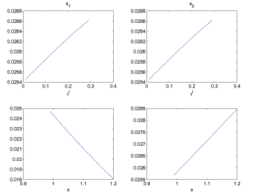
The second reason that a CCK type of argument does not carry over to our environment is that search frictions also result in welfare costs of anticipated inflation absent in a standard model. In a standard model, long-run inflation simply distorts the marginal rate of substitution between cash and credit goods. In our model, long-run inflation also affects the household shopping margin between cash search goods and credit search goods. Here, it is helpful to think in terms of the household shopping margin that we constructed in (11). In a high-inflation (and hence high nominal interest rate) steady state, the return to searching for and entering into a long-run credit relationship is greater than the return to searching for and entering into a long-run cash relationship, simply because the latter requires the use of money, whose value erodes with inflation, while the former does not. Substituting (7) into (11) and imposing steady state shows that a higher "regular" nominal interest rate $R$, ceteris paribus, results in a lower shadow nominal interest rate $R^{*}$.¹⁸ With $R^{*}$ defined as the relative probability $k^{h}(\theta _{2})/k^{h}(\theta_{1})$ a household matches in the credit market versus in the cash market, anticipated inflation thus directs household search away from the cash sector and towards the credit sector. We confirm these effects in the bottom row of Figure 4 by plotting the long-run responses of $s_{1}$ and $s_{2}$ to exogenous changes in the inflation rate (governed by the long-run money growth rate), holding the labor tax fixed at $\tau^{l}=0$. In summary, labor income taxation and anticipated inflation have consequences for search-market outcomes that a standard model cannot articulate, and these effects are important in shaping the Ramsey policy.

Appendix F  Restoring the Friedman Rule Through Alternative Instruments

The deviation from the Friedman Rule is due to two distinct reasons, each related to recent results in the optimal policy literature: a positive nominal interest rate indirectly taxes firm profits and also serves to guide search markets towards efficiency. To assess the contribution of each of these auxiliary roles of the nominal interest rate to the magnitude of the departure from the Friedman Rule, we introduce in succession two alternative tax instruments to the environment.

First, we allow the Ramsey planner access to a proportional tax on profit income. The way in which we allow for a profit tax follows closely Schmitt-Grohe and Uribe (2004a): we assume that household receipts of dividend payments by firms are taxed at the rate $\tau^{pr}_{t}$. Formally, in the household flow budget constraint (2), we modify the last term on the right hand side to read $(1-\tau^{pr}_{t-1}) P_{t-1} d_{t-1}$. Note that the presence of this profit tax does not affect any of the private-sector equilibrium conditions -- because households take $d_{t}$ as given -- which is the key to understanding how it operates. The way in which the profit tax alters the PVIC is shown at the end of Appendix D.

As in Schmitt-Grohe and Uribe (2004a), assuming a natural upper bound of $\tau^{pr}$ of 100 percent, it is easy to show that the Ramsey planner would set $\tau^{pr}=1$ because that achieves maximum relaxation of the PVIC.¹⁹ The third row of Table 1 shows that with a 100 percent profit tax, the nominal interest rate falls from 5.65 percent to 3.18 percent. The labor income tax rate also falls because part of revenue is now raised through the profit tax, but we still have $\tau^{l} > 0$. Thus, over 2 percent of the positive nominal interest rate in the second row of Table 1 is a proxy for a profit tax. Just as in Schmitt-Grohe and Uribe (2004a), Ramsey taxation of profits is non-distortionary in our environment, hence desirable. Taxation of long-run profit flows are non-distortionary in our environment because the pre-determined customer bases $N_{1}$ and $N_{2}$, which are the source of firm revenue and hence profit, cannot be altered.²⁰ In the absence of a direct tax on this fixed profit flow, the nominal interest rate can indirectly tax it. The fact that the nominal interest rate falls upon introduction of a profit tax is thus consistent with Schmitt-Grohe and Uribe (2004a); the fact that it does not fall all the way to zero is different from their result. There is thus yet another motivation for setting a positive nominal interest rate in our environment.

This second motivation stems from inefficiently-high $s_{1}$ and $s_{2}$ induced by the positive labor income tax, an effect we documented, recall, for the exogenous-policy case in the top row of Figure 4. The natural instrument to correct inefficiently-high search is a tax directly on search. Denote by $\tau^{s_{1} }$ ( $\tau^{s_{2}}$) a proportional tax on cash (credit) search activity. We introduce search taxation by including $\tau^{s_{1}}_{t-1} s_{1t-1} + \tau^{s_{2}}_{t-1} s_{2t-1}$ on the left-hand-side of the household budget constraint (2). For generality, we allow for differential search taxation, reflected in our notation, on cash search and credit search, but it turns out that $\tau^{s_{1}} = \tau^{s_{2}}$. Unlike the profit tax, search taxes do affect equilibrium conditions. Specifically, they modify the equilibrium versions of the cash and credit shopping conditions to

$$\frac{g^{\prime}_{t} + u_{2t} \tau^{s_{i}}_{t}}{k^{h}(\theta_{it})} = \beta(1-\rho^{x}) E_{t} \left\{ c_{it+1}\left[ \vartheta v_{it+1} - p_{it+1} u_{it+1}\right] - g^{\prime}_{t+1} + \frac{g^{\prime}_{t+1} + u_{2t+1} \tau^{s_{i}}_{t+1}}{k^{h}(\theta_{it+1})} \right\} ,$$ (91)

for $i = 1,2$, which is a straightforward and intuitive modification of the shopping conditions (9) and (10): search taxes add to the marginal cost of searching (the left-hand-side), but also add to the expected future marginal benefit of successfully forming a customer relationship (the right-hand-side) by allowing the household to save on future search taxes. We also introduce $\tau^{s_{1}}_{t} s_{1t} + \tau^{s_{2}}_{t} s_{2t}$ as a revenue item in the government budget constraint, making it part of the optimal government financing problem. This means that the PVIC includes the search taxes; we show at the end of Appendix D how search taxes alter the PVIC.

Optimizing directly in the Ramsey problem with respect to $\tau^{s_{1}}_{t}$ and $\tau^{s_{2}}_{t}$, we find the optimal steady-state search tax rates are $\tau^{s_{1}} = \tau^{s_{2}} = 0.48$. At first glance, this seems quite high, but on further reflection one realizes that because we do not seem to observe search taxes at all in reality, there really is no basis for judging whether or not it is "high." In any case, our main interest here is not in the search taxes themselves, but rather in what their presence implies for the rest of the Ramsey policy mix. The bottom row of Table 1 presents the Ramsey policy and allocation in the presence of these search taxes and the 100-percent profit tax. The most important result here is that optimality of the Friedman Rule is restored. We omit it from the table, but we also computed the Ramsey solution in the presence of just search taxes and $\tau^{pr} = 0$. Here, we found $100(R - 1)= 5.6601$ (virtually identical to that in the second row of Table 1), $\tau^{l} = 0.2198$, $\tau^{s_{1}} = 0.5593$, and $\tau^{s_{2}} = 0.7258$. Thus, both profit taxes and search taxes are required to restore the optimality of the Friedman Rule. The deviation from the Friedman Rule in our environment thus has connections with the findings of both Schmitt-Grohe and Uribe (2004a) and with those of Cooley and Quadrini (2004), Arseneau and Chugh (2007a), and Rocheteau and Wright (2005).

In terms of welfare, steady-state utility (not shown) is strictly increasing as we move down Table 1 from the Ramsey equilibrium with neither profit nor search taxes to the Ramsey equilibrium with profit taxes but no search taxes to the Ramsey equilibrium with both profit and search taxes. Qualitatively examining how allocations vary as instruments are successively added, it is clear that allocations move closer to the Pareto optimum shown in the first row of Table 1. Of course, the Ramsey equilibrium can never get all the way to the Pareto optimum because $\tau^{l} > 0$ is required under any Ramsey equilibrium.

Having demonstrated that positive nominal interest rates proxy for multiple instruments in our environment, the main analysis in the text omits these alternative instruments. Our reason for omitting the alternative instruments is that in studying Ramsey dynamics, given that we drop the ZLB constraint from the dynamic solution, we want to ensure our equilibrium does not pierce the zero lower bound during simulations. Results obtained by Cooley and Quadrini (2004) and Arseneau and Chugh (2007a) suggest that causing such a level-shift in policy in this way does not blur interpretation of dynamics.

Appendix G  Varying Search Parameters

It is interesting to examine how the Ramsey equilibrium varies with a few novel parameters associated with search markets. Figures 5 and 6 analyze the Ramsey steady state along the bargaining-power dimension, plotting key policy and allocation variables as a function of customer bargaining power $\eta$. Varying $\eta$ away from 0.5 moves the economy away from the usual notion of Hosios efficiency. This type of departure from search efficiency is the one most related to the existing labor-search or money-search literature, in contrast to our demonstration above that labor-income taxation also makes outcomes in search markets inefficient, which is a more novel, policy-induced, type of departure from Hosios efficiency.²¹

Based on our results that the optimal nominal interest rate can proxy for direct search taxes, it is natural to expect that the nominal interest rate will vary with $\eta$. Indeed, as the upper left panel of Figure 5 shows, the optimal nominal interest rate is increasing in $\eta$. This response arises because the Ramsey government tries to mitigate households' increased search activity induced by higher $\eta$. Absent the policy response shown in the upper left panel of Figure 5, the rise in the sum of $s_{1}$ and $s_{2}$ (each of which is shown in Figure 6) would be even larger, which we can confirm by running the corresponding experiments in the exogenous (non-Ramsey) policy environment.²² In terms of how other allocation variables vary with $\eta$ (i.e., $a_{1}$ and $a_{2}$ depend negatively on $\eta$, $p_{1}$ and $p_{2}$ depend negatively on $\eta$, and so on), the results in Figures 5 and 6 match up with those of Arseneau and Chugh (2007b), so we refer the reader there for more analysis.

Figure 5:  Steady-state Ramsey policy and allocation variables as function of customer bargaining power $\eta$.

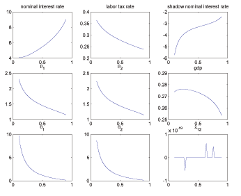
Figure 6  Steady-state Ramsey policy and allocation variables as function of customer bargaining power $\eta$.

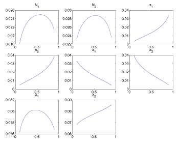
Figures 7 and 8 display how the Ramsey steady-state depends on $\vartheta$, which, recall from the specification of household preferences in (1), governs how valuable search goods are to the household. In the absence of direct evidence, recall that we set as our baseline $\vartheta= 1$. Setting $\vartheta= 0$ eliminates search markets and collapses our model to a standard CCK cash/credit economy. The optimal nominal interest rate, shown in the upper left panel of Figure 7, rises as $\vartheta$ rises because profits generated from search markets (not shown) grow with $\vartheta$. A larger profit base makes taxing profits more attractive to the Ramsey planner, and we already showed above that the nominal interest rate has the ability to indirectly tax profits. The responses of search-market allocation variables as $\vartheta$ rises (i.e., $N_{i}$, $a_{i}$, and $s_{i}$, $i=1,2$, all increase) all are intuitive: the more important (all) search goods are in preferences, the more resources the economy directs to search activities.

Figure 7:  Steady-state Ramsey policy and allocation variables as function of importance of search goods, governed by $\vartheta$.

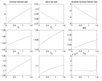
Figure 8:  Steady-state Ramsey policy and allocation variables as function of importance of search goods, governed by $\vartheta$.

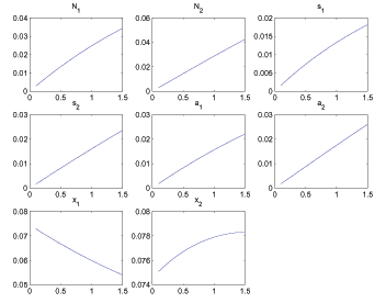
Finally, our baseline calibration has $\kappa_{c} = \kappa_{x} = 0.5$, meaning the importance of cash and credit goods in preferences is symmetric across search and non-search markets. A natural conjecture may be that cash transactions are less important in markets with long-lived relationships. Because of repeat interactions, a firm may be more willing to "extend credit" to a good customer. We can probe this idea by varying $\kappa_{c}$, holding all other parameters fixed at their baseline values; Figures 9 and 10 plot the Ramsey steady state as we vary $\kappa_{c}$. Higher values of $\kappa_{c}$ mean that cash is less intensively used for goods acquired in bilateral transactions. The results are again quite intuitive. As $\kappa_{c}$ rises, cash search goods are valued less and less, so activity in the cash search market disappears, as evidenced by the fact that $N_{1}$ (the number of active cash relationships), $s_{1}$ (the number of individuals searching for cash goods), and $a_{1}$ (advertisements posted in the cash search market) all tend towards zero. For $\kappa_{c} > 0.6$, the ZLB binds, revealed by the fact that the Ramsey multiplier on the ZLB constraint (denoted $\lambda_{12}$ and displayed in the lower right panel of Figure 9) rises above zero.

Figure 9:  Steady-state Ramsey policy and allocation variables as function of share parameter $\kappa_{c}$.

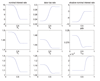
Figure 10:  Steady-state Ramsey policy and allocation variables as function of share parameter $\kappa_{c}$.

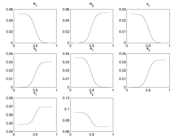
References

Arseneau, David M. and Sanjay K. Chugh. 2006. "Ramsey Meets Hosios: The Optimal Capital Tax and Labor Market Efficiency." International Finance Discussion Paper no. 870, Board of Governors of the Federal Reserve System.

Arseneau, David M. and Sanjay K. Chugh. 2007a. "Optimal Fiscal and Monetary Policy with Costly Wage Bargaining." International Finance Discussion Paper no. 893, Board of Governors of the Federal Reserve System.

Arseneau, David M. and Sanjay K. Chugh. 2007b. "Bargaining, Fairness, and Price Rigidity in a DSGE Environment." International Finance Discussion Paper no. 898, Board of Governors of the Federal Reserve System.

Aruoba, S. Boragan and Sanjay K. Chugh. 2006. "Optimal Fiscal and Monetary Policy When Money is Essential." International Finance Discussion Paper no. 880, Board of Governors of the Federal Reserve System.

Blinder, Alan S., Elier D. Canetti, David E. Lebow, and Jeremy B. Rudd. 1998. Asking About Prices: A New Approach to Understanding Price Stickiness. Russell Sage Foundation.

Chugh, Sanjay K. 2006. "Optimal Fiscal and Monetary Policy with Sticky Wages and Sticky Prices." Review of Economic Dynamic, Vol. 9, pp. 683-714.

Chugh, Sanjay K. 2007a. "Optimal Inflation Persistence: Ramsey Taxation with Capital and Habits." Journal of Monetary Economics, Vol. 54, pp. 1809-1836.

Chugh, Sanjay K. 2007b. "Does the Timing of the Cash-in-Advance Constraint Matter for Optimal Fiscal and Monetary Policy?." University of Maryland.

Cooley, Thomas F. and Vincenzo Quadrini. 2004. "Optimal Monetary Policy in a Phillips-Curve World." Journal of Economic Theory, Vol. 118, pp. 174-208.

Fabiani, Silvia, Martine Druant, Ignacio Hernando, Claudia Kwapil, Bettina Landau, Claire Loupias, Fernando Martins, Thomas Matha, Roberto Sabbatini, Harald Stahl, and Ad Stokman. 2006. "What Firms' Surveys Tell Us About Price-Setting Behavior in the Euro Area." International Journal of Central Banking, Vol. 2, pp. 3-47.

Hall, Robert E. 2007. "Equilibrium Sticky Prices." Stanford University.

Hosios, Arthur J. 1990. "On the Efficiency of Matching and Related Models of Search and Unemployment." Review of Economic Studies, Vol. 57, pp. 279-298.

Khan, Aubhik, Robert G. King and Alexander L. Wolman. 2003. "Optimal Monetary Policy." Review of Economic Studies, Vol. 70, pp. 825-860.

King, Robert G. and Sergio T. Rebelo. 1999. "Resuscitating Real Business Cycles." In Handbook of Macroeconomics, John B. Taylor and Michael Woodford, Vol. 1B. Elsevier.

Kishor, N. Kundan and Levis A. Kochin. 2007. "The Success of the Fed and the Death of Monetarism." Economic Inquiry, Vol. 45, pp. 56-70.

Kleshchelski, Isaac and Nicolas Vincent. 2007. "Market Share and Price Rigidity." Northwestern University.

Lagos, Ricardo and Randall Wright. 2005. "A Unified Framework for Monetary Theory and Policy Analysis." Journal of Political Economy, Vol. 113, pp. 463-484.

Lucas, Robert E. Jr. and Nancy L. Stokey. 1983. "Optimal Fiscal and Monetary Policy in an Economy Without Capital." Journal of Monetary Economics, Vol. 12, pp. 55-93.

Nakamura, Emi and Jon Steinsson. 2007. "Price Setting in Forward-Looking Customer Markets." Harvard University.

Pissarides, Christopher A. 2000. Equilibrium Unemployment Theory. MIT Press.

Ravn, Morten, Stephanie Schmitt-Grohe, and Martin Uribe. 2006. "Deep Habits." Review of Economic Studies, Vol. 73, pp. 195-218.

Rocheteau, Guillaume and Randall Wright. 2005. "Money in Search equilibrium, in Competitive Equilibrium, and in Competitive Search Equilibrium." Econometrica, Vol. 73, pp. 175-202.

Rogerson, Richard, Robert Shimer, and Randall Wright. 2005. "Search-Theoretic Models of the Labor Market: A Survey." Journal of Economic Literature, Vol. 43, pp. 959-988.

Schmitt-Grohe, Stephanie and Martin Uribe. 2004a. "Optimal Fiscal and Monetary Policy Under Imperfect Competition." Journal of Macroeconomics, Vol. 26, pp. 183-209.

Schmitt-Grohe, Stephanie and Martin Uribe. 2004b. "Optimal Fiscal and Monetary Policy Under Sticky Prices." Journal of Economic Theory, Vol. 114, pp. 198-230.

Schmitt-Grohe, Stephanie and Martin Uribe. 2004c. "Solving Dynamic General Equilibrium Models Using a Second-Order Approximation to the Policy Function." Journal of Economic Dynamics and Control, Vol. 28, pp. 755-775.

Schmitt-Grohe, Stephanie and Martin Uribe. 2005. "Optimal Fiscal and Monetary Policy in a Medium-Scale Macroeconomic Model." NBER Macroeconomics Annual 2005.

Footnotes

^†  Email address: [email protected]. Return to text

^‡  Email address: [email protected]. Return to text

1.  For example, even if one knows exactly where to go to buy certain goods, one may still have to walk around the aisles, stand in the checkout line, etc. Return to text

2.  One crucial way in which our environment is different from Lagos and Wright (2005) and related models is that during the course of a long-term relationship, a customer and a firm are not anonymous. Anonymity of buyers and sellers is a crucial feature underlying the role for money in money-search types of models. Return to text

3.  To keep things symmetric, we assume $\rho^{x}$ is identical across cash and credit relationships, and, as we present below, we assume a number of other features of the environment are symmetric across the two types of relationships. One could easily relax such assumptions, but we think it makes the most sense to begin with as symmetric an environment as possible. Return to text

4.  Echoing a point we made earlier, allowing $\gamma$ to differ across the two markets might be another natural feature in which to introduce asymmetry across cash and credit relationships. Return to text

5.  Technically, of course, it is the real interest rate with which firms discount profits, and in equilibrium the real interest rate between time zero and time $t$ is measured by $\Xi_{t\vert}$. Because there will be no confusion using this equilibrium result "too early," we skip this intermediate level of notation and structure. Return to text

6.  Again, more details are provided in Appendices A and B. Return to text

7.  For example, the advertising expenditures -- a colorful banner, a hand-written sign showing sale prices -- of a hot dog vendor one goes to every day, one that accepts only cash, on a street corner of New York City probably do not get recorded in advertising data. Return to text

8.  Recall from the household shopping conditions (9) and (10) that $g^{\prime}(.)$ measures the marginal cost of shopping. Return to text

9.  The "fixed factor" in our model arises from the search and matching frictions, which generate local monopolies between customers and firms. Return to text

10.  From their simulation experiments, Chari and Kehoe (1999) report a mean inflation rate of -0.44 percent with a standard deviation of 19.93; Schmitt-Grohe and Uribe (2004a) report a mean inflation rate of -3.39 percent with a standard deviation of 7.47 percent; Siu (2004) reports a mean inflation rate of -2.59 percent with a standard deviation of 5.08 percent; and Chugh (2006) reports a mean inflation rate of -4.01 percent with a standard deviation of 6.96 percent. Each of these models is calibrated in a slightly different way from the others, but the general result that comes through is clear: with flexible prices, the Ramsey inflation rate is quite volatile. Return to text

11.  The Hosios (1990) proof also depends on constant returns to scale in matching, which Cobb-Douglas matching of course satisfies. Return to text

12.  In particular, given the symmetry across differentiated intermediate goods built into the Dixit-Stiglitz aggregator commonly employed in modern sticky-price models, unanticipated inflation would give rise to relative price distortions across producers, which would then lead to an inefficient mix of goods production. See, for example, Woodford (2003, p. 406). Return to text

13.  Formally, the way in which we construct this restricted-Ramsey equilibrium is to impose the constraint $R_{t} = \bar{R}$ when solving for the dynamics of the model, where $\bar{R}$ is the (unrestricted) Ramsey-optimal steady-state nominal interest rate. Return to text

14.  Simply because of the Ramsey assumption that no direct lump-sum instruments of any sort exist. Thus, $\pi$ and $\tau^{l}$ are tightly linked through the government budget constraint, as is the case in any Ramsey monetary model. Return to text

15.  Recall from the household shopping conditions (9) and (10) that $g^{\prime}(.)/k^{h}(.)$ measures the marginal cost of shopping. Return to text

16.  To emphasize, Figure 4 presents non-Ramsey responses. Return to text

17.  Cobb-Douglas matching means that firm matching rates $k^{f}(\theta_{i})$ increase as $\theta_{i}$ falls. For brevity, we do not plot all of these equilibrium responses, but we have confirmed them. Return to text

18.  The ceteris paribus is important here; as we show below in an experiment where we vary the parameter $\eta$, a positive association between $R$ and $R^{*}$ can arise in the Ramsey equilibrium. It is of course more difficult to make analytical statements regarding the Ramsey equilibrium because the binding government budget constraint renders very few things ceteris paribus. This is a general statement about Ramsey models, not one about just our model. Return to text

19.  More precisely, maximum relaxation of the PVIC would occur at that profit tax rate at which the multiplier on the PVIC in the Ramsey problem is zero. At this profit tax rate, the planner would be able to implement a zero labor income tax rate because all government spending would be financed through the non-distortionary profit tax. In our baseline model, the profit tax rate at which the Ramsey multiplier on the PVIC shrinks to zero is 140 percent. This result is not very interesting because it means that we effectively are no longer considering a Ramsey equilibrium, defined as one in which at least some distortionary instruments must be used. Hence the natural cap on $\tau^{pr}$ at 100 percent. Schmitt-Grohe and Uribe (2004a) also impose this natural upper limit, but we suspect that an unconstrained optimization over $\tau^{pr}$ must similarly yield $\tau^{pr} > 1$ in their model. Return to text

20.  In Schmitt-Grohe and Uribe (2004a), the fixity of firm profits stems from the exogenous Dixit-Stiglitz-style monopoly power firms wield. Return to text

21.  Arseneau and Chugh (2006) also demonstrate that policy-induced departures from Hosios efficiency lead to auxiliary roles for other "standard" tax instruments; their focus was on a capital income tax. Return to text

22.  Specifically, in the exogenous-policy environment, we find, computationally, $\partial s_{i} / \partial\eta> 0$, $i=1,2$, which is intuitive (a higher return to search, measured by higher bargaining power, induces a household to increase its search), and also that $\partial s / \partial\pi< 0$, where $s = s_{1} + s_{2}$. The latter can also be seen in the bottom row of Figure 4, in which $s_{1}$ falls by more than $s_{2}$ rises as $\pi$ rises, meaning $s_{1} + s_{2}$ falls. Return to text

This version is optimized for use by screen readers. Descriptions for all mathematical expressions are provided in LaTex format. A printable pdf version is available. Return to text

Home | Economic research and data | Publications and education resources
Accessibility | Contact us
Last update: February 7, 2008