
Board of Governors of the Federal Reserve System
International Finance Discussion Papers
Number 938, July 2008--- Screen Reader
Version*
Political Disagreement, Lack of Commitment and the Level of Debt*
NOTE: International Finance Discussion Papers are preliminary materials circulated to stimulate discussion and critical comment. References in publications to International Finance Discussion Papers (other than an acknowledgment that the writer has had access to unpublished material) should be cleared with the author or authors. Recent IFDPs are available on the Web at http://www.federalreserve.gov/pubs/ifdp/. This paper can be downloaded without charge from the Social Science Research Network electronic library at http://www.ssrn.com/.
Abstract:
We analyze how public debt evolves when successive policymakers have different policy goals and cannot make credible commitments about their future policies. We consider several cases to be able to disentangle and quantify the respective effects of imperfect commitment and political disagreement. Absent political turnover, imperfect commitment drives the long-run level of debt to zero. With political disagreement, debt is a sizeable fraction of GDP and increasing in the degree of polarization among parties, no matter the degree of commitment. The frequency of political turnover does not produce quantitatively relevant effects. These results are consistent with much of the existing empirical evidence. Finally, we find that in the presence of political disagreement the welfare gains of building commitment are lower.
Keywords: Time-consistency, political disagreement
JEL classification: C61, E61, E62, P16
1 Introduction
1.1 Motivation
In the fiscal policy literature, there is not a clear theoretical understanding of the forces driving the observed patterns of public debt. This paper explores how debt evolves when governments cannot make credible commitments about future policies and when policymakers with different policy goals alternate in office. We consider several cases to be able to disentangle and quantify the respective effects of imperfect commitment and political disagreement.
As it is well known, the evolution of debt matters in a world where the provision of public goods has to be financed by raising distortionary taxes.1 In this context, as shown e.g. in the works of Barro (1979), Lucas and Stokey (1983) and Aiyagari et al. (2002), debt is used to smooth over time the deadweight losses associated with such distortions. These models can account for many aspects of the evolution of debt for many countries. However, these theories do not provide a complete explanation of some basic and stylized facts, like why public debt is a sizeable fraction of GDP in many developed countries and why there is a substantial variation in the debt/GDP ratio across countries with similar economic conditions.2
In macroeconomic models, the optimal (second-best) allocations are usually characterized as the solution to a Ramsey problem. It is assumed that the same planner is always in charge and that he can commit to future policies, maximizing the welfare of an infinitely lived representative agent.3 Under these assumptions and with complete financial markets, as shown by Lucas and Stokey (1983), the long-run level of debt crucially depends on the initial conditions.4 Countries starting with high debt will have high debt forever, and countries with low debt will have low debt forever. Since initial conditions are exogenous to the model and empirically difficult to determine, such a theory can not explain what induces countries to accumulate debt.
Policymaking in practice departs from the idealized environment described in Lucas and Stokey (1983) in many dimensions. In this work, we investigate how imperfect commitment and disagreement among successive policymakers can provide an incentive to accumulate debt. There are important reasons to think that these two forces may considerably affect the behavior of debt.
First, the role of commitment is related to the time-inconsistency problem in optimal policy choices, as illustrated in the seminal works of Kydland and Prescott (1977) and Barro and Gordon (1983). In our context, the solution under full-commitment is time inconsistent because a planner, at a given point in time, is willing to abandon his previous plans to manipulate the interest rate. For example, if the planner needs to issue debt, he has an incentive to reduce the interest rate. Hence, the planner is willing to lower current taxes, in order to foster current consumption. Because of a smoothing motive, this leads to an increase in the demand for savings and thus to a reduction in the interest rate. As a consequence, because of the lower tax revenues, in a one-time deviation from the full-commitment solution, the planner runs deficits and accumulates debt.5 Therefore, it seems worth exploring how debt evolves when the planner cannot make credible commitments about his future policies.6 We thus check whether a positive long-run level of debt may be the outcome of the optimal policy under the no-commitment assumption and other imperfect commitment settings.
Second, some studies in the political economy literature (see e.g. Alesina and Tabellini (1990) and Persson and Svensson (1989)), have emphasized how the presence of political disagreement may provide incentives to accumulate an inefficient level of debt. In a world characterized by political disagreement, the assumption of full-commitment seems unrealistic. Due to this reason, the literature assumed that governments always lack commitment. However, it would still be reasonable to assume that governments may have commitment during their tenures, but cannot commit on behalf of their successors, who have different objectives. In this paper, we consider a framework with political disagreement among successive policymakers, where commitment plays an important role in the strategic game between policymakers and private agents.7 In this context, the incumbent policymaker makes different choices depending on his ability to commit while staying in office. This allows us to explicitly analyze the effects of commitment in a world with political disagreement among successive policymakers.
We build on the simple Lucas and Stokey (1983) model, introducing endogenous government expenditure, which has to be financed by raising a proportional income tax and/or by issuing debt. We develop a framework that allows us to disentangle and quantify the effects of imperfect commitment, frequency of turnover and political disagreement in a dynamic context. In this respect, our contribution is methodological. Our framework can be used to analyze the effects of commitment in a wide set of infinite-horizon optimal policy problems, where policymakers with different objectives alternate in office. In other words, the methodology developed here allows us to integrate the analysis about the time-inconsistency of optimal policy choices, typical of the dynamic macroeconomic literature, into a political economy model. By doing so, we are able to measure the implications of building commitment in the presence of political disagreement.
From an economic point of view, the main contribution and findings of our analysis are the following. First, abstracting from political disagreement, we study the optimal fiscal policy under the no-commitment assumption. Under a wide set of initial conditions and parameterizations, we find that debt goes to zero in the long-run. Perhaps surprisingly, this means that there is a striking difference in the behavior of debt in a one-time deviation from commitment and in the no-commitment (time-consistent) solution. As we will discuss later, reducing debt over time is the only way the planner with no-commitment can favorably affect the interest rate.
Second, we study the behavior of debt in cases where the planner has access to a commitment technology, but under some circumstances, say because of political pressures, big shocks etc., he may renege on his past promises. This is what we call the loose commitment setting. Because of the striking difference in the behavior of debt between the full-commitment and the no-commitment cases, it seems worth checking how debt evolves under loose commitment. We find that in this last case the level of debt still converges to zero in the long-run. This suggests that the steady-state dependency on initial conditions found in Lucas and Stokey (1983) is not robust to small deviations from the full-commitment case. In addition, our results suggest that departing from the full-commitment assumption cannot help explaining why the level of debt is a sizeable fraction of GDP.
Third, we also find that debt is increased in periods when the planner reneges on his past promises and reduced over the periods of commitment.
This result is interesting since it suggests that the simple expectation that the planner may surprise the economy at a future date induces him to commit to reduce debt over time.
Fourth, we investigate one case where the imperfect commitment assumption is natural, i.e. when successive planners have different policy goals. We find that in the presence of political disagreement, debt is a sizeable fraction of GDP, regardless of the commitment assumptions. In our numerical exercises, political disagreement seems to be the main driving force for accumulating deficits. On the contrary, the effects of imperfect commitment and political turnover have a small impact on the level of debt. Our predictions are consistent with most of the existing empirical evidence. Indeed, while there is a large consensus on the positive relationship between the degree of political polarization and debt accumulation, the empirical findings about the effects of the frequency of political turnover are less clear-cut. More importantly, our results suggest that when testing empirically the effects of political instability on the level of debt, it is important to control both for measures of polarization among parties and measures of political turnover, rather than using any of them as a generic indicator of political instability.
Finally, when analyzing welfare implications, we find that the gains from commitment are lower in the presence of political disagreement than in a no-disagreement case. From an intuitive point of view, this happens because in the absence of political disagreement governments with more commitment will maximize overall social welfare. However, with political disagreement a better commitment technology can be used by each party to maximize specific groups' welfare.
1.2 Related literature
Krusell et al. (2006) analyze the time-consistent solution of the otherwise standard Lucas and Stokey (1983) model, where government expenditures are exogenous. The authors find as a solution a multiplicity of steady-states and discontinuous policy functions, where debt adjusts for one or two periods and then remains constant. Their main finding is that under no-commitment the equilibrium is close to the solution under commitment. In our paper, we also build on the Lucas and Stokey (1983) model, but consider the case where government expenditure is endogenous. The presence of this additional instrument in the hands of the policymaker widens the set of his feasible choices. In section 3, we extensively discuss how this makes a difference. We obtain continuous policy functions, and we find that in the absence of commitment debt goes to zero. This result is surprising because it is usually the case that in a one-time deviation from commitment debt increases.
In the literature, several papers have analyzed the effects of lack of commitment on debt in monetary economies. When nominal debt is present, the monetary authority usually has an incentive to raise the price level to reduce the real value of the outstanding debt. The first period of the full-commitment solution reveals such incentives, since debt is eroded in real terms. Martin (2006a) and Diaz-Gimenez et al. (2006) analyze monetary economies under discretion where the cash-in-advance constraint is key to determine the level of debt. They find that the steady-state level of debt can be positive, negative or zero depending on the parametrization of the utility function. If it is easy (difficult) for households to substitute cash goods then government holds assets (debt).8 As in Krusell et al. (2006) we focus on a real economy without a cash-in-advance constraint. Since in most countries central banks are independent and committed to price stability, we believe that focusing on a real economy is a reasonable assumption. Our result that debt converges to zero is not due to the presence of nominal bonds nor it is achieved with surprise inflation.
Some studies in the political economy literature, like Alesina and Tabellini (1990), have analyzed how policy decisions are formulated when policymakers with different political views alternate in office. Azimonti-Renzo (2004), as we do here, extends the previous works to an infinite horizon problem, but in a context where commitment about future policy does not affect private agents' choices. The author considers a fiscal policy model with balanced budget, and public but no private capital. Instead, we focus on the effects of political disagreement on the level of government debt. Our main contribution with respect to this literature is to study optimal policy where commitment plays a role in the strategic interactions between agents and the policymakers. Moreover, we solve the problem under different commitment settings. We indeed consider the case where parties cannot commit at all, but we also assume that parties can credibly commit for the future, in case they are reappointed in office. This allows to disentangle and quantify the effects of imperfect commitment, political disagreement and frequency of political turnover on the level of debt. Finally, it allows to measure the welfare gains from commitment in the presence of political disagreement.
In recent work, Song et al. (2006) and Battaglini and Coate (2008) study the evolution of debt in a dynamic political economy framework, and provide an explanation for the presence of a long-run positive level of debt. They consider models with political conflicts over public goods redistribution, either across generations or across geographical districts. In these works, however, the interest rate is exogenous and the commitment problem arises because of repeated voting. In our work, we instead study an infinite horizon problem, where the disagreement is about the composition of a public good, while considering a simpler voting mechanism. More importantly, we analyze a case where policy choices are time-inconsistent because of the policymaker's incentive to manipulate the interest rate, which would be present even in the absence of repeated voting or political turnover. In such context, we study the strategic interactions between policymakers with different objectives alternating in office.
The paper is organized as follows: in section 2 we introduce the model and, as a benchmark for our analysis, we recover the solution under full-commitment. In section 3, we describe the solution under no-commitment, i.e. the time-consistent solution. In section 4, we illustrate the behavior of debt under the less extreme assumption of loose commitment. In section 5, we study the joint implications of political disagreement and imperfect commitment and we compare our findings with the existing empirical literature. Finally, we discuss welfare implications. Section 6 concludes.
2 The model
We build our analysis on a simple model, as in Lucas and Stokey (1983), where time-inconsistency issues arise.
For the time being, we abstract from uncertainty and political
disagreement between successive governments.9 We consider an
economy where labor is the only factor of production, and
technology is linear, and output can be used either for private
consumption ![]() or for public consumption
or for public consumption
![]() . The economy's aggregate budget
constraint is therefore
. The economy's aggregate budget
constraint is therefore
| (1) |
The public good is provided by a benevolent government and
financed through a proportional tax ![]() on labor
income and by issuing a one-period bond
on labor
income and by issuing a one-period bond ![]() with
price
with
price ![]() . At any point in time, the government
budget constraint is
. At any point in time, the government
budget constraint is
| (2) |
In a decentralized equilibrium, given taxes, prices and the quantities of public expenditure, the representative household chooses consumption, savings and leisure by solving the following problem:

|
|
|
| (3) |
where ![]() is the price at time
is the price at time ![]() of private bond holdings (
of private bond holdings (![]() ), paying
one unit of consumption at time t+1.
), paying
one unit of consumption at time t+1.
The household's first order conditions are
| (4) | ||
 |
(5) |
together with the budget constraint (3). Equation (4) and (5) represent the equilibrium condition in the labor market and the bond market, respectively.
In what follows, we analyze the problem of the government and characterize its solution under the assumption of full-commitment. This will serve as a benchmark for our discussion in subsequent sections.
2.1 The case of full-commitment
If the government has full-commitment, for a given initial level
of debt (![]() ), it solves the following problem
), it solves the following problem
|
||
| (6) |
where we made use of the household's optimality conditions
(3)-(5), the resource
constraint (1) and the market
clearing condition
![]() , to substitute for
taxes, public expenditure, leisure and government debt. We rule out
Ponzi schemes, by imposing the transversality condition
, to substitute for
taxes, public expenditure, leisure and government debt. We rule out
Ponzi schemes, by imposing the transversality condition
| (7) |
For our purposes it is worth recalling some features of the
resulting equilibrium. As discussed in Lucas and Stokey (1983), in the full-commitment case after an
initial jump, all the allocations, including the amount of debt,
reach their steady-state level, and remain constant from then on.
This is because, apart from ![]() , all the periods
are identical and the government is willing to smooth private and
public consumption over time. However, the steady-state allocations
depend on the initial condition
, all the periods
are identical and the government is willing to smooth private and
public consumption over time. However, the steady-state allocations
depend on the initial condition ![]() . In other
words, countries starting with high debt will have high debt
forever, and countries with low debt will have low debt forever.
Because of this dependency on initial conditions, which are
exogenous to the model and empirically difficult to determine, this
theory cannot explain why countries accumulate debt to start with.
Moreover, it cannot explain why the level of debt is so different
across countries with similar economic conditions.
. In other
words, countries starting with high debt will have high debt
forever, and countries with low debt will have low debt forever.
Because of this dependency on initial conditions, which are
exogenous to the model and empirically difficult to determine, this
theory cannot explain why countries accumulate debt to start with.
Moreover, it cannot explain why the level of debt is so different
across countries with similar economic conditions.
The first-period allocations are different, because of the
time-inconsistency problem typical of this setting. The government,
when making its plans at period ![]() , would like to
use taxes and public expenditure to manipulate the bond price. This
is because of the following. For a generic
, would like to
use taxes and public expenditure to manipulate the bond price. This
is because of the following. For a generic ![]() ,
current consumption influences both
,
current consumption influences both ![]() and
and
![]() . As a consequence, if the government
uses taxes and public expenditure to increase the price of the bond
. As a consequence, if the government
uses taxes and public expenditure to increase the price of the bond
![]() , other things equal, it also decreases
, other things equal, it also decreases
![]() . At an optimum, it turns out that the
costs of such a procedure offset the benefits. However, at
. At an optimum, it turns out that the
costs of such a procedure offset the benefits. However, at
![]() things are different, because consumers'
savings and previous prices (
things are different, because consumers'
savings and previous prices (![]() ) are given.
Therefore, if the government inherits a positive level of debt, it
can benefit from an increase in the price of the bond without
incurring any additional cost. For example, by setting its policies
such that current consumption is higher than in the future, the
government is able to foster the demand for savings, thus selling
bonds at a more convenient price.10 These incentives to
increase initial consumption prevail whenever the government is
allowed to make a new plan. This is why the solution to this
problem is in general time-inconsistent.
) are given.
Therefore, if the government inherits a positive level of debt, it
can benefit from an increase in the price of the bond without
incurring any additional cost. For example, by setting its policies
such that current consumption is higher than in the future, the
government is able to foster the demand for savings, thus selling
bonds at a more convenient price.10 These incentives to
increase initial consumption prevail whenever the government is
allowed to make a new plan. This is why the solution to this
problem is in general time-inconsistent.
Figure 1: Debt dynamics under full-commitment
Note: The figure plots, for different level of initial debt, the level of consumption in the first period (solid line) and the steady-state level of consumption (dashed line). The reported values correspond to the calibration specified in table A-2.
Data for Figure 1
| Probability | Consumption at steady state | Initial Consumption |
|---|---|---|
| 0.00 | 0.24682 | 0.24682 |
| 0.25 | 0.24361 | 0.25940 |
| 0.50 | 0.24087 | 0.27259 |
| 0.75 | 0.23853 | 0.28527 |
| 1.00 | 0.23648 | 0.29707 |
To explain better the mechanism described above, in figure
1 we plot the
level of consumption at ![]() (
(![]() ) and
the steady-state level of consumption (
) and
the steady-state level of consumption (![]() ), for a
given positive initial level of debt (
), for a
given positive initial level of debt (
![]() ), under the full-commitment
assumption.11 We can see that the higher is debt,
the bigger is the difference between current and future
consumption, and thus the higher is the drop in the interest rate.
This happens because the higher is debt the larger is the base on
which the improved interest rate is applied. As a consequence, the
higher is the inherited level of debt, the greater is the
willingness to manipulate the interest rate.
), under the full-commitment
assumption.11 We can see that the higher is debt,
the bigger is the difference between current and future
consumption, and thus the higher is the drop in the interest rate.
This happens because the higher is debt the larger is the base on
which the improved interest rate is applied. As a consequence, the
higher is the inherited level of debt, the greater is the
willingness to manipulate the interest rate.
Now we can look at the behavior of debt in the first period, by
looking at the government budget constraint in equation (2).
On the one hand, the tax cut necessary to foster initial
consumption reduces the tax revenues of the government. On the
other hand, the resulting lower interest rate allows the government
to sell bonds at a higher price. Whether
![]() depends on the composite
effect of these two forces. In figure 2, we plot the
level of debt chosen in the first period (and thus the steady-state
level of debt), as a function of
depends on the composite
effect of these two forces. In figure 2, we plot the
level of debt chosen in the first period (and thus the steady-state
level of debt), as a function of ![]() . For low
levels of
. For low
levels of ![]() , the government accumulates debt.
However, if the initial level of debt is large enough, the increase
in bond prices applies to a larger base. As a consequence, the tax
cut can be self-financed and the level of debt can also
decrease.
, the government accumulates debt.
However, if the initial level of debt is large enough, the increase
in bond prices applies to a larger base. As a consequence, the tax
cut can be self-financed and the level of debt can also
decrease.
Figure 2: Debt dynamics under full-commitment
Note: The figure plots the steady-state level of debt (bs s), that is the level of debt prevailing from the first period on, as a function of the initial debt (b0). The reported values correspond to the parameterization specified in table A-2.
3 The time-consistent solution
In this section, we analyze the problem of a benevolent planner which, as opposed to the case of the previous section, does not have access to a commitment technology. More precisely, we consider the case in which the current planner cannot make credible promises about his future actions. We keep the assumption that the planner can credibly commit to repay his loans.12 In what follows, we also assume that reputation mechanisms are not operative, focusing only on Markov-Perfect equilibria, as defined for instance in Klein et al. (2004).
In this case the problem of the planner is
| (8) | ||
| (9) |
The function
![]() in constraint (9)
determines the quantity of consumption the consumer expects for
period
in constraint (9)
determines the quantity of consumption the consumer expects for
period ![]() as a function of the debt level
as a function of the debt level
![]() outstanding at the beginning of next
period. This represents the main difference with respect to the
full-commitment case. Since the current planner cannot make
credible commitments about his future actions, the future stream of
consumption is not under his direct control. By taking as given the
policy
outstanding at the beginning of next
period. This represents the main difference with respect to the
full-commitment case. Since the current planner cannot make
credible commitments about his future actions, the future stream of
consumption is not under his direct control. By taking as given the
policy
![]() of his successor (or himself in
the next period), the current planner can only influence future
consumption through his current debt policy. Being the function
of his successor (or himself in
the next period), the current planner can only influence future
consumption through his current debt policy. Being the function
![]() unknown, the solution of this
problem relies on solving a fixed point problem in
unknown, the solution of this
problem relies on solving a fixed point problem in
![]() .13
.13
We can now look at the first order conditions of the associated Lagrangian, and in particular at the generalized Euler equation (GEE)
| (10) |
where
![]() indicates the Lagrange multiplier
attached to constraint (9).14
indicates the Lagrange multiplier
attached to constraint (9).14![]() 15 The
inspection of the previous equation allows us to describe the
behavior of the economy in a (deterministic) steady-state. In
particular, for the GEE to be satisfied in steady-state, it must be
that
15 The
inspection of the previous equation allows us to describe the
behavior of the economy in a (deterministic) steady-state. In
particular, for the GEE to be satisfied in steady-state, it must be
that
| (11) |
We can identify three different cases in which such relationship holds, as illustrated in figure 3. This figure, together with the steady-states implied by eq. (11), gives a qualitative representation of the transition dynamics obtained in our numerical experiments.
Figure 3: Debt dynamics in the time-consistent Case
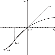
Note: The figure is a qualitative representation of debt equilibrium dynamics resulting from our numerical experiments.
First, we have the case in which ![]() . This
means that constraint (9)
is not binding, and we are at an unconstrained optimum. From an
economic point of view, this is saying that the planner can avoid
to raise distortionary taxes and can finance his public expenditure
through the interest payments received on his outstanding assets.
This represents the first-best solution.16
. This
means that constraint (9)
is not binding, and we are at an unconstrained optimum. From an
economic point of view, this is saying that the planner can avoid
to raise distortionary taxes and can finance his public expenditure
through the interest payments received on his outstanding assets.
This represents the first-best solution.16
Second, we have the case in which
![]() . This can happen when a marginal
change in the level of debt does not induce any change in the
equilibrium level of private consumption. This case cannot be ruled
out. However, given the presence of distortionary taxation, this is
not due to Ricardian equivalence. On the contrary, when a planner
inherits a higher level of debt, he has to raise more distortionary
taxes. Because of the bigger distortions created, by a substitution
effect, this will reduce hours worked and private consumption. An
increase in debt also creates a wealth effect that decreases hours
worked and increases private consumption.
. This can happen when a marginal
change in the level of debt does not induce any change in the
equilibrium level of private consumption. This case cannot be ruled
out. However, given the presence of distortionary taxation, this is
not due to Ricardian equivalence. On the contrary, when a planner
inherits a higher level of debt, he has to raise more distortionary
taxes. Because of the bigger distortions created, by a substitution
effect, this will reduce hours worked and private consumption. An
increase in debt also creates a wealth effect that decreases hours
worked and increases private consumption.
Both the wealth and substitution effects lead to a reduction in
hours worked as debt increases. The composite effect on private
consumption can be understood by examining the aggregate resource
constraint. By differentiating equation (1) with respect to
debt (![]() ) it holds
) it holds
|
(12) |
In a model where public expenditure is exogenous, the effects on
consumption must be equal to the ones on hours worked. As a
consequence, in such case, ![]() cannot be
zero. But in our framework, there is another way for the planner to
cope with the higher burden created by the higher debt. That is, by
reducing the amount of public good provision. As a result, it is
possible that a marginal change in the level of debt does not
produce any effect on the level of equilibrium consumption (i.e.
cannot be
zero. But in our framework, there is another way for the planner to
cope with the higher burden created by the higher debt. That is, by
reducing the amount of public good provision. As a result, it is
possible that a marginal change in the level of debt does not
produce any effect on the level of equilibrium consumption (i.e.
![]() ) as long as the effects on leisure
(
) as long as the effects on leisure
(![]() ) and public expenditure (
) and public expenditure (![]() )
exactly offset each other.
)
exactly offset each other.
Finally, we have a steady-state, associated with a level of debt equal to zero. When debt is zero, the government does not have any incentive to manipulate the interest rate. At this point, policymakers' commitment is irrelevant and thus debt remains constant at a zero level, as in the full-commitment case.
We now turn to explain the transition dynamics of the model. Under full-commitment, after the initial period debt is constant. With no-commitment the pictures change significantly and this is due temptation to influence the interest rate not only in the first period, as in the full-commitment case, but in every period. As illustrated in Figure 3 we find that, in the (more relevant) cases in which the government initially holds a positive amount of debt or relatively small amount of assets, the economy will converge to the steady-state with zero debt.
As explained for the full-commitment case, whenever a government
inherits a positive amount of debt, it has the incentive to use the
instruments at its disposal to reduce the interest rate payments
or, equivalently, to increase the selling price of bonds, as given
by (5). To
do so, the demand for savings should increase, which will happen if
current consumption increases more than future consumption. A
government with full-commitment could promise the desired level of
future consumption regardless of the debt level, as long as the
allocation is feasible. In the no-commitment case this is no longer
true. The government can only influence future actions through the
state variables, which in our case is debt. The higher the
inherited debt, the higher will be the incentive in the next period
to increase consumption again, in order to manipulate bond prices.
Therefore, to face favorable bond prices, the current government
needs to leave a lower debt to its successor. If it does not do so,
the successor will raise consumption even more, and the anticipated
positive consumption growth would harm the current bond price. It
follows that debt is reduced until a level of zero debt is reached.
At this point, the incentive to manipulate the interest rate
vanishes. A symmetric argument also explains why a government that
starts with assets, but to the right of the point where
![]() , would instead reduce the asset
holdings to manipulate the bond price, until the zero debt level is
reached.
, would instead reduce the asset
holdings to manipulate the bond price, until the zero debt level is
reached.
The mechanism that we explained above relies on the temptation
that every government has to manipulate the bond price. If a
government reduces debt, then tomorrow's government will face a
smaller temptation to manipulate the bond price, and consequently
consumption will be lower than today's. However, there is a second
effect. As we mentioned before, when debt is lowered, the
government can afford to lower taxes. As a consequence, leisure
decreases, output increases and the economy can increase both
private and public consumption. According to this effect, if
tomorrow's government has lower debt then it will increase private
consumption. Notice that this second effect goes in an opposite
direction of the first one. At the point
![]() the two effects exactly cancel
out. To the left of
the two effects exactly cancel
out. To the left of
![]() the second effect dominates, i.e.
when assets are accumulated (debt is reduced) consumption
increases. The amount of debt at which
the second effect dominates, i.e.
when assets are accumulated (debt is reduced) consumption
increases. The amount of debt at which
![]() depends on the marginal rate of
substitution between private and public consumption and between
consumption and leisure.17 Under our baseline calibration, as
it can be seen in Figure 3 the point where
depends on the marginal rate of
substitution between private and public consumption and between
consumption and leisure.17 Under our baseline calibration, as
it can be seen in Figure 3 the point where
![]() is associated with government
asset holdings (
is associated with government
asset holdings (![]() ). In this case, the
steady-state with
). In this case, the
steady-state with
![]() is unstable, while the steady
state with
is unstable, while the steady
state with ![]() is stable.18
is stable.18
From a theoretical point of view, it is also possible to have
![]() at a point where debt is positive.
In that case, such steady-state with positive debt is stable, while
the steady-state with
at a point where debt is positive.
In that case, such steady-state with positive debt is stable, while
the steady-state with ![]() is unstable. In other
words, whenever the government starts with debt it would converge
to the point
is unstable. In other
words, whenever the government starts with debt it would converge
to the point
![]() . And, whenever the government
starts with assets it would accumulate further assets, until public
expenditures can be financed only through the associated interest
payments. In our numerical exercises, we found that for
calibrations implying a plausible level of public expenditure the
case depicted in Figure 3 is the relevant
one. In particular, one can obtain that the steady-state with zero
debt is unstable only when the steady-state public expenditures are
unreasonably low.19 In what follows we abstract from
considering these cases and focus on the case where the
steady-state with
. And, whenever the government
starts with assets it would accumulate further assets, until public
expenditures can be financed only through the associated interest
payments. In our numerical exercises, we found that for
calibrations implying a plausible level of public expenditure the
case depicted in Figure 3 is the relevant
one. In particular, one can obtain that the steady-state with zero
debt is unstable only when the steady-state public expenditures are
unreasonably low.19 In what follows we abstract from
considering these cases and focus on the case where the
steady-state with ![]() is stable.
is stable.
To provide a more concrete description of the behavior of our economy, we solve the model numerically by assuming the following functional form for the utility function:20
![$\displaystyle u(c,x,g)=(1-\phi_{g})\left[ \phi_{c}\frac{c^{1-\sigma_{c}}-1}{1-\sigma_{c} }+(1-\phi_{c})\frac{x^{1-\sigma_{x}}-1}{1-\sigma_{x}}\right] +\phi_{g} \frac{g^{1-\sigma_{g}}-1}{1-\sigma_{g}},$](img82.gif)
|
(13) |
where ![]() and
and ![]() denote
the preference weights on private and public consumption.
denote
the preference weights on private and public consumption.
We use a standard calibration for an annualized model of the US economy in order to match long-run ratios of our variables. Table A-2 summarizes the parameter values.21
The evolution of the allocations over time is illustrated in figures 4 and 5 where, for comparison, we also display the solution under full-commitment. For a given level of initial debt, we can observe a decreasing pattern of private consumption and an increasing interest rate.22 This is achieved by lowering taxation and increasing public consumption over time.
Figure 4: Commitment vs. no-commitment: time pattern of allocations
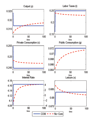
Note: The figure plots the equilibrium allocations over time, giving an initial condition of b = .16 which is roughly 50% of GDP under our parameterization. The interest rate (lower-left panel) for the full-commitment case (continuous line) has to be referred to the right-hand scale.
Data for Figure 4
| Time | Output: Discretion | Output: Commitment | Taxes: Discretion | Taxes: Commitment | Private Consumption: Discretion | Private Consumption: Commitment | Public Consumption: Discretion | Public Consumption: Commitment | Leisure: Discretion | Leisure: Commitment |
|---|---|---|---|---|---|---|---|---|---|---|
| 0 | 0.3127 | 0.3241 | 0.2398 | 0.1598 | 0.2484 | 0.2547 | 0.0643 | 0.0694 | 0.6873 | 0.6759 |
| 1 | 0.3130 | 0.3168 | 0.2395 | 0.2490 | 0.2483 | 0.2447 | 0.0647 | 0.0720 | 0.6870 | 0.6832 |
| 2 | 0.3133 | 0.3168 | 0.2391 | 0.2490 | 0.2482 | 0.2447 | 0.0651 | 0.0720 | 0.6867 | 0.6832 |
| 3 | 0.3135 | 0.3168 | 0.2388 | 0.2490 | 0.2481 | 0.2447 | 0.0654 | 0.0720 | 0.6865 | 0.6832 |
| 4 | 0.3137 | 0.3168 | 0.2385 | 0.2490 | 0.2481 | 0.2447 | 0.0657 | 0.0720 | 0.6863 | 0.6832 |
| 5 | 0.3139 | 0.3168 | 0.2382 | 0.2490 | 0.2480 | 0.2447 | 0.0660 | 0.0720 | 0.6861 | 0.6832 |
| 6 | 0.3141 | 0.3168 | 0.2379 | 0.2490 | 0.2479 | 0.2447 | 0.0662 | 0.0720 | 0.6859 | 0.6832 |
| 7 | 0.3143 | 0.3168 | 0.2377 | 0.2490 | 0.2479 | 0.2447 | 0.0664 | 0.0720 | 0.6857 | 0.6832 |
| 8 | 0.3145 | 0.3168 | 0.2374 | 0.2490 | 0.2478 | 0.2447 | 0.0667 | 0.0720 | 0.6855 | 0.6832 |
| 9 | 0.3146 | 0.3168 | 0.2372 | 0.2490 | 0.2478 | 0.2447 | 0.0669 | 0.0720 | 0.6854 | 0.6832 |
| 10 | 0.3148 | 0.3168 | 0.2369 | 0.2490 | 0.2477 | 0.2447 | 0.0670 | 0.0720 | 0.6852 | 0.6832 |
| 11 | 0.3149 | 0.3168 | 0.2367 | 0.2490 | 0.2477 | 0.2447 | 0.0672 | 0.0720 | 0.6851 | 0.6832 |
| 12 | 0.3151 | 0.3168 | 0.2365 | 0.2490 | 0.2477 | 0.2447 | 0.0674 | 0.0720 | 0.6849 | 0.6832 |
| 13 | 0.3152 | 0.3168 | 0.2363 | 0.2490 | 0.2476 | 0.2447 | 0.0675 | 0.0720 | 0.6848 | 0.6832 |
| 14 | 0.3153 | 0.3168 | 0.2361 | 0.2490 | 0.2476 | 0.2447 | 0.0677 | 0.0720 | 0.6847 | 0.6832 |
| 15 | 0.3154 | 0.3168 | 0.2359 | 0.2490 | 0.2476 | 0.2447 | 0.0678 | 0.0720 | 0.6846 | 0.6832 |
| 16 | 0.3155 | 0.3168 | 0.2357 | 0.2490 | 0.2475 | 0.2447 | 0.0680 | 0.0720 | 0.6845 | 0.6832 |
| 17 | 0.3156 | 0.3168 | 0.2355 | 0.2490 | 0.2475 | 0.2447 | 0.0681 | 0.0720 | 0.6844 | 0.6832 |
| 18 | 0.3157 | 0.3168 | 0.2354 | 0.2490 | 0.2475 | 0.2447 | 0.0682 | 0.0720 | 0.6843 | 0.6832 |
| 19 | 0.3158 | 0.3168 | 0.2352 | 0.2490 | 0.2475 | 0.2447 | 0.0683 | 0.0720 | 0.6842 | 0.6832 |
| 20 | 0.3159 | 0.3168 | 0.2350 | 0.2490 | 0.2474 | 0.2447 | 0.0684 | 0.0720 | 0.6841 | 0.6832 |
| 21 | 0.3160 | 0.3168 | 0.2349 | 0.2490 | 0.2474 | 0.2447 | 0.0685 | 0.0720 | 0.6840 | 0.6832 |
| 22 | 0.3160 | 0.3168 | 0.2347 | 0.2490 | 0.2474 | 0.2447 | 0.0686 | 0.0720 | 0.6840 | 0.6832 |
| 23 | 0.3161 | 0.3168 | 0.2346 | 0.2490 | 0.2474 | 0.2447 | 0.0687 | 0.0720 | 0.6839 | 0.6832 |
| 24 | 0.3162 | 0.3168 | 0.2344 | 0.2490 | 0.2474 | 0.2447 | 0.0688 | 0.0720 | 0.6838 | 0.6832 |
| 25 | 0.3163 | 0.3168 | 0.2343 | 0.2490 | 0.2474 | 0.2447 | 0.0689 | 0.0720 | 0.6837 | 0.6832 |
| 26 | 0.3163 | 0.3168 | 0.2342 | 0.2490 | 0.2473 | 0.2447 | 0.0690 | 0.0720 | 0.6837 | 0.6832 |
| 27 | 0.3164 | 0.3168 | 0.2340 | 0.2490 | 0.2473 | 0.2447 | 0.0691 | 0.0720 | 0.6836 | 0.6832 |
| 28 | 0.3165 | 0.3168 | 0.2339 | 0.2490 | 0.2473 | 0.2447 | 0.0692 | 0.0720 | 0.6835 | 0.6832 |
| 29 | 0.3165 | 0.3168 | 0.2338 | 0.2490 | 0.2473 | 0.2447 | 0.0692 | 0.0720 | 0.6835 | 0.6832 |
| 30 | 0.3166 | 0.3168 | 0.2337 | 0.2490 | 0.2473 | 0.2447 | 0.0693 | 0.0720 | 0.6834 | 0.6832 |
| 31 | 0.3166 | 0.3168 | 0.2336 | 0.2490 | 0.2473 | 0.2447 | 0.0694 | 0.0720 | 0.6834 | 0.6832 |
| 32 | 0.3167 | 0.3168 | 0.2335 | 0.2490 | 0.2473 | 0.2447 | 0.0694 | 0.0720 | 0.6833 | 0.6832 |
| 33 | 0.3167 | 0.3168 | 0.2334 | 0.2490 | 0.2473 | 0.2447 | 0.0695 | 0.0720 | 0.6833 | 0.6832 |
| 34 | 0.3168 | 0.3168 | 0.2333 | 0.2490 | 0.2472 | 0.2447 | 0.0696 | 0.0720 | 0.6832 | 0.6832 |
| 35 | 0.3168 | 0.3168 | 0.2332 | 0.2490 | 0.2472 | 0.2447 | 0.0696 | 0.0720 | 0.6832 | 0.6832 |
| 36 | 0.3169 | 0.3168 | 0.2331 | 0.2490 | 0.2472 | 0.2447 | 0.0697 | 0.0720 | 0.6831 | 0.6832 |
| 37 | 0.3169 | 0.3168 | 0.2330 | 0.2490 | 0.2472 | 0.2447 | 0.0697 | 0.0720 | 0.6831 | 0.6832 |
| 38 | 0.3170 | 0.3168 | 0.2329 | 0.2490 | 0.2472 | 0.2447 | 0.0698 | 0.0720 | 0.6830 | 0.6832 |
| 39 | 0.3170 | 0.3168 | 0.2328 | 0.2490 | 0.2472 | 0.2447 | 0.0698 | 0.0720 | 0.6830 | 0.6832 |
| 40 | 0.3171 | 0.3168 | 0.2327 | 0.2490 | 0.2472 | 0.2447 | 0.0699 | 0.0720 | 0.6829 | 0.6832 |
| 41 | 0.3171 | 0.3168 | 0.2326 | 0.2490 | 0.2472 | 0.2447 | 0.0699 | 0.0720 | 0.6829 | 0.6832 |
| 42 | 0.3171 | 0.3168 | 0.2325 | 0.2490 | 0.2472 | 0.2447 | 0.0700 | 0.0720 | 0.6829 | 0.6832 |
| 43 | 0.3172 | 0.3168 | 0.2324 | 0.2490 | 0.2472 | 0.2447 | 0.0700 | 0.0720 | 0.6828 | 0.6832 |
| 44 | 0.3172 | 0.3168 | 0.2324 | 0.2490 | 0.2472 | 0.2447 | 0.0701 | 0.0720 | 0.6828 | 0.6832 |
| 45 | 0.3173 | 0.3168 | 0.2323 | 0.2490 | 0.2471 | 0.2447 | 0.0701 | 0.0720 | 0.6827 | 0.6832 |
| 46 | 0.3173 | 0.3168 | 0.2322 | 0.2490 | 0.2471 | 0.2447 | 0.0702 | 0.0720 | 0.6827 | 0.6832 |
| 47 | 0.3173 | 0.3168 | 0.2321 | 0.2490 | 0.2471 | 0.2447 | 0.0702 | 0.0720 | 0.6827 | 0.6832 |
| 48 | 0.3174 | 0.3168 | 0.2321 | 0.2490 | 0.2471 | 0.2447 | 0.0702 | 0.0720 | 0.6826 | 0.6832 |
| 49 | 0.3174 | 0.3168 | 0.2320 | 0.2490 | 0.2471 | 0.2447 | 0.0703 | 0.0720 | 0.6826 | 0.6832 |
| 50 | 0.3174 | 0.3168 | 0.2319 | 0.2490 | 0.2471 | 0.2447 | 0.0703 | 0.0720 | 0.6826 | 0.6832 |
| 51 | 0.3175 | 0.3168 | 0.2318 | 0.2490 | 0.2471 | 0.2447 | 0.0703 | 0.0720 | 0.6825 | 0.6832 |
| 52 | 0.3175 | 0.3168 | 0.2318 | 0.2490 | 0.2471 | 0.2447 | 0.0704 | 0.0720 | 0.6825 | 0.6832 |
| 53 | 0.3175 | 0.3168 | 0.2317 | 0.2490 | 0.2471 | 0.2447 | 0.0704 | 0.0720 | 0.6825 | 0.6832 |
| 54 | 0.3175 | 0.3168 | 0.2316 | 0.2490 | 0.2471 | 0.2447 | 0.0705 | 0.0720 | 0.6825 | 0.6832 |
| 55 | 0.3176 | 0.3168 | 0.2316 | 0.2490 | 0.2471 | 0.2447 | 0.0705 | 0.0720 | 0.6824 | 0.6832 |
| 56 | 0.3176 | 0.3168 | 0.2315 | 0.2490 | 0.2471 | 0.2447 | 0.0705 | 0.0720 | 0.6824 | 0.6832 |
| 57 | 0.3176 | 0.3168 | 0.2315 | 0.2490 | 0.2471 | 0.2447 | 0.0706 | 0.0720 | 0.6824 | 0.6832 |
| 58 | 0.3177 | 0.3168 | 0.2314 | 0.2490 | 0.2471 | 0.2447 | 0.0706 | 0.0720 | 0.6823 | 0.6832 |
| 59 | 0.3177 | 0.3168 | 0.2313 | 0.2490 | 0.2471 | 0.2447 | 0.0706 | 0.0720 | 0.6823 | 0.6832 |
| 60 | 0.3177 | 0.3168 | 0.2313 | 0.2490 | 0.2471 | 0.2447 | 0.0706 | 0.0720 | 0.6823 | 0.6832 |
| 61 | 0.3177 | 0.3168 | 0.2312 | 0.2490 | 0.2471 | 0.2447 | 0.0707 | 0.0720 | 0.6823 | 0.6832 |
| 62 | 0.3178 | 0.3168 | 0.2312 | 0.2490 | 0.2471 | 0.2447 | 0.0707 | 0.0720 | 0.6822 | 0.6832 |
| 63 | 0.3178 | 0.3168 | 0.2311 | 0.2490 | 0.2471 | 0.2447 | 0.0707 | 0.0720 | 0.6822 | 0.6832 |
| 64 | 0.3178 | 0.3168 | 0.2311 | 0.2490 | 0.2470 | 0.2447 | 0.0708 | 0.0720 | 0.6822 | 0.6832 |
| 65 | 0.3178 | 0.3168 | 0.2310 | 0.2490 | 0.2470 | 0.2447 | 0.0708 | 0.0720 | 0.6822 | 0.6832 |
| 66 | 0.3178 | 0.3168 | 0.2310 | 0.2490 | 0.2470 | 0.2447 | 0.0708 | 0.0720 | 0.6822 | 0.6832 |
| 67 | 0.3179 | 0.3168 | 0.2309 | 0.2490 | 0.2470 | 0.2447 | 0.0708 | 0.0720 | 0.6821 | 0.6832 |
| 68 | 0.3179 | 0.3168 | 0.2309 | 0.2490 | 0.2470 | 0.2447 | 0.0709 | 0.0720 | 0.6821 | 0.6832 |
| 69 | 0.3179 | 0.3168 | 0.2308 | 0.2490 | 0.2470 | 0.2447 | 0.0709 | 0.0720 | 0.6821 | 0.6832 |
| 70 | 0.3179 | 0.3168 | 0.2308 | 0.2490 | 0.2470 | 0.2447 | 0.0709 | 0.0720 | 0.6821 | 0.6832 |
| 71 | 0.3179 | 0.3168 | 0.2307 | 0.2490 | 0.2470 | 0.2447 | 0.0709 | 0.0720 | 0.6821 | 0.6832 |
| 72 | 0.3180 | 0.3168 | 0.2307 | 0.2490 | 0.2470 | 0.2447 | 0.0709 | 0.0720 | 0.6820 | 0.6832 |
| 73 | 0.3180 | 0.3168 | 0.2307 | 0.2490 | 0.2470 | 0.2447 | 0.0710 | 0.0720 | 0.6820 | 0.6832 |
| 74 | 0.3180 | 0.3168 | 0.2306 | 0.2490 | 0.2470 | 0.2447 | 0.0710 | 0.0720 | 0.6820 | 0.6832 |
| 75 | 0.3180 | 0.3168 | 0.2306 | 0.2490 | 0.2470 | 0.2447 | 0.0710 | 0.0720 | 0.6820 | 0.6832 |
| 76 | 0.3180 | 0.3168 | 0.2305 | 0.2490 | 0.2470 | 0.2447 | 0.0710 | 0.0720 | 0.6820 | 0.6832 |
| 77 | 0.3181 | 0.3168 | 0.2305 | 0.2490 | 0.2470 | 0.2447 | 0.0711 | 0.0720 | 0.6819 | 0.6832 |
| 78 | 0.3181 | 0.3168 | 0.2304 | 0.2490 | 0.2470 | 0.2447 | 0.0711 | 0.0720 | 0.6819 | 0.6832 |
| 79 | 0.3181 | 0.3168 | 0.2304 | 0.2490 | 0.2470 | 0.2447 | 0.0711 | 0.0720 | 0.6819 | 0.6832 |
| 80 | 0.3181 | 0.3168 | 0.2304 | 0.2490 | 0.2470 | 0.2447 | 0.0711 | 0.0720 | 0.6819 | 0.6832 |
| 81 | 0.3181 | 0.3168 | 0.2303 | 0.2490 | 0.2470 | 0.2447 | 0.0711 | 0.0720 | 0.6819 | 0.6832 |
| 82 | 0.3181 | 0.3168 | 0.2303 | 0.2490 | 0.2470 | 0.2447 | 0.0711 | 0.0720 | 0.6819 | 0.6832 |
| 83 | 0.3182 | 0.3168 | 0.2303 | 0.2490 | 0.2470 | 0.2447 | 0.0712 | 0.0720 | 0.6818 | 0.6832 |
| 84 | 0.3182 | 0.3168 | 0.2302 | 0.2490 | 0.2470 | 0.2447 | 0.0712 | 0.0720 | 0.6818 | 0.6832 |
| 85 | 0.3182 | 0.3168 | 0.2302 | 0.2490 | 0.2470 | 0.2447 | 0.0712 | 0.0720 | 0.6818 | 0.6832 |
| 86 | 0.3182 | 0.3168 | 0.2301 | 0.2490 | 0.2470 | 0.2447 | 0.0712 | 0.0720 | 0.6818 | 0.6832 |
| 87 | 0.3182 | 0.3168 | 0.2301 | 0.2490 | 0.2470 | 0.2447 | 0.0712 | 0.0720 | 0.6818 | 0.6832 |
| 88 | 0.3182 | 0.3168 | 0.2301 | 0.2490 | 0.2470 | 0.2447 | 0.0712 | 0.0720 | 0.6818 | 0.6832 |
| 89 | 0.3182 | 0.3168 | 0.2300 | 0.2490 | 0.2470 | 0.2447 | 0.0713 | 0.0720 | 0.6818 | 0.6832 |
| 90 | 0.3183 | 0.3168 | 0.2300 | 0.2490 | 0.2470 | 0.2447 | 0.0713 | 0.0720 | 0.6817 | 0.6832 |
| 91 | 0.3183 | 0.3168 | 0.2300 | 0.2490 | 0.2470 | 0.2447 | 0.0713 | 0.0720 | 0.6817 | 0.6832 |
| 92 | 0.3183 | 0.3168 | 0.2299 | 0.2490 | 0.2470 | 0.2447 | 0.0713 | 0.0720 | 0.6817 | 0.6832 |
| 93 | 0.3183 | 0.3168 | 0.2299 | 0.2490 | 0.2470 | 0.2447 | 0.0713 | 0.0720 | 0.6817 | 0.6832 |
| 94 | 0.3183 | 0.3168 | 0.2299 | 0.2490 | 0.2470 | 0.2447 | 0.0713 | 0.0720 | 0.6817 | 0.6832 |
| 95 | 0.3183 | 0.3168 | 0.2299 | 0.2490 | 0.2470 | 0.2447 | 0.0714 | 0.0720 | 0.6817 | 0.6832 |
| 96 | 0.3183 | 0.3168 | 0.2298 | 0.2490 | 0.2470 | 0.2447 | 0.0714 | 0.0720 | 0.6817 | 0.6832 |
| 97 | 0.3183 | 0.3168 | 0.2298 | 0.2490 | 0.2470 | 0.2447 | 0.0714 | 0.0720 | 0.6817 | 0.6832 |
| 98 | 0.3184 | 0.3168 | 0.2298 | 0.2490 | 0.2470 | 0.2447 | 0.0714 | 0.0720 | 0.6816 | 0.6832 |
| 99 | 0.3184 | 0.3168 | 0.2297 | 0.2490 | 0.2470 | 0.2447 | 0.0714 | 0.0720 | 0.6816 | 0.6832 |
Figure 5: Commitment vs. no-commitment: time pattern of debt
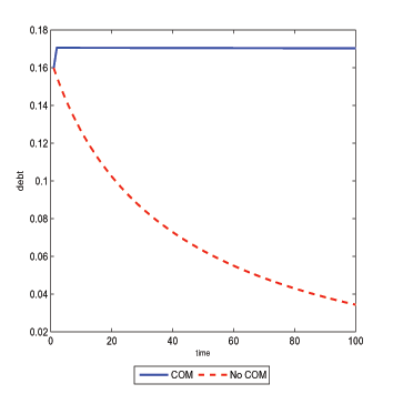
Note: The figure plots the evolution of debt over time, giving an initial condition of b = .16 which is roughly 50% of GDP under our parameterization. The solid line corresponds to the full-commitment case, while the dashed line corresponds to the no-commitment case.
Data for Figure 5
| Time | Discretion | Commitment |
|---|---|---|
| 1 | 0.160 | 0.160 |
| 2 | 0.155 | 0.171 |
| 3 | 0.151 | 0.171 |
| 4 | 0.147 | 0.171 |
| 5 | 0.143 | 0.171 |
| 6 | 0.139 | 0.171 |
| 7 | 0.136 | 0.171 |
| 8 | 0.133 | 0.171 |
| 9 | 0.129 | 0.171 |
| 10 | 0.126 | 0.171 |
| 11 | 0.124 | 0.171 |
| 12 | 0.121 | 0.171 |
| 13 | 0.118 | 0.171 |
| 14 | 0.116 | 0.171 |
| 15 | 0.113 | 0.171 |
| 16 | 0.111 | 0.171 |
| 17 | 0.109 | 0.171 |
| 18 | 0.107 | 0.171 |
| 19 | 0.104 | 0.171 |
| 20 | 0.102 | 0.171 |
| 21 | 0.100 | 0.171 |
| 22 | 0.099 | 0.171 |
| 23 | 0.097 | 0.171 |
| 24 | 0.095 | 0.171 |
| 25 | 0.093 | 0.171 |
| 26 | 0.092 | 0.171 |
| 27 | 0.090 | 0.171 |
| 28 | 0.089 | 0.171 |
| 29 | 0.087 | 0.171 |
| 30 | 0.086 | 0.171 |
| 31 | 0.084 | 0.171 |
| 32 | 0.083 | 0.171 |
| 33 | 0.081 | 0.171 |
| 34 | 0.080 | 0.171 |
| 35 | 0.079 | 0.171 |
| 36 | 0.078 | 0.171 |
| 37 | 0.076 | 0.171 |
| 38 | 0.075 | 0.171 |
| 39 | 0.074 | 0.171 |
| 40 | 0.073 | 0.171 |
| 41 | 0.072 | 0.171 |
| 42 | 0.071 | 0.171 |
| 43 | 0.070 | 0.171 |
| 44 | 0.069 | 0.171 |
| 45 | 0.068 | 0.171 |
| 46 | 0.067 | 0.171 |
| 47 | 0.066 | 0.171 |
| 48 | 0.065 | 0.171 |
| 49 | 0.064 | 0.171 |
| 50 | 0.063 | 0.171 |
| 51 | 0.062 | 0.171 |
| 52 | 0.061 | 0.171 |
| 53 | 0.060 | 0.171 |
| 54 | 0.060 | 0.171 |
| 55 | 0.059 | 0.171 |
| 56 | 0.058 | 0.171 |
| 57 | 0.057 | 0.171 |
| 58 | 0.057 | 0.171 |
| 59 | 0.056 | 0.171 |
| 60 | 0.055 | 0.171 |
| 61 | 0.054 | 0.171 |
| 62 | 0.054 | 0.171 |
| 63 | 0.053 | 0.171 |
| 64 | 0.052 | 0.171 |
| 65 | 0.052 | 0.171 |
| 66 | 0.051 | 0.171 |
| 67 | 0.050 | 0.171 |
| 68 | 0.050 | 0.171 |
| 69 | 0.049 | 0.171 |
| 70 | 0.049 | 0.171 |
| 71 | 0.048 | 0.171 |
| 72 | 0.047 | 0.171 |
| 73 | 0.047 | 0.171 |
| 74 | 0.046 | 0.171 |
| 75 | 0.046 | 0.171 |
| 76 | 0.045 | 0.171 |
| 77 | 0.045 | 0.171 |
| 78 | 0.044 | 0.171 |
| 79 | 0.044 | 0.171 |
| 80 | 0.043 | 0.171 |
| 81 | 0.043 | 0.171 |
| 82 | 0.042 | 0.171 |
| 83 | 0.042 | 0.171 |
| 84 | 0.041 | 0.171 |
| 85 | 0.041 | 0.171 |
| 86 | 0.040 | 0.171 |
| 87 | 0.040 | 0.171 |
| 88 | 0.039 | 0.171 |
| 89 | 0.039 | 0.171 |
| 90 | 0.038 | 0.171 |
| 91 | 0.038 | 0.171 |
| 92 | 0.038 | 0.171 |
| 93 | 0.037 | 0.171 |
| 94 | 0.037 | 0.171 |
| 95 | 0.036 | 0.171 |
| 96 | 0.036 | 0.171 |
| 97 | 0.036 | 0.171 |
| 98 | 0.035 | 0.171 |
| 99 | 0.035 | 0.171 |
| 100 | 0.034 | 0.171 |
In the initial period, in the no-commitment case taxes are higher and public consumption is lower than in the full-commitment case. Such policies allow not only to foster private consumption in the desired way, but also to run a surplus. As a result debt decreases over time. As the level of debt and interest payments are reduced, public consumption is raised and taxes are reduced. This will make consumers work more and consume less over time.
As discussed above, it is feasible to have lower taxes and lower levels of private consumption only if the level of public consumption is increased. In a model where public expenditure is exogenously determined, for example, it will not be possible to have lower taxes and lower consumption at the same time. In that context, for an exogenously given amount of public expenditure, lower taxes will imply a higher amount of hours worked and thus, by the resource constraint, higher consumption.23 This prevents having a decreasing pattern of consumption and reducing debt at the same time.
Our results suggests that with no-commitment the exposure of the government in terms of debt/assets will be lower than in the case of full-commitment. This result may seem counterintuitive when compared with our discussion about the temptation to deviate from full-commitment (see section 2.1). In general, however, there is no reason why the policy with no-commitment should mimic the policy implemented in a one-time deviation from full-commitment. In the commitment case, the planner can benefit from the interest rate manipulation simply by taxing less today, and promising that future consumption will be lower, regardless of the level of debt. In the case of no-commitment, the government realizes that in order to conveniently manipulate the interest rate, it has to leave a lower debt to its successor. Thus debt decreases over time.
To summarize, we find that debt dynamics are very different depending on the specific assumptions about commitment. In the absence of commitment, under the more plausible calibrations and initial conditions, debt converges to zero in the long-run. From a positive point of view, both the full commitment and the no commitment case are unappealing. In the former case, the level of debt crucially depends on initial conditions, while in the latter case the implication of the model of zero long-run debt is clearly at odds with the empirical evidence.
4 Loose commitment
As shown in the previous sections, the evolution of debt changes dramatically depending on whether we assume full-commitment or no-commitment. Both cases are clearly extreme depictions of reality. As it seems more realistic, in this section we analyze the case where a benevolent policymaker has the ability to commit but, under some circumstances (like wars, political pressures, etc.), it may renege on its past promises. We refer to this case as loose commitment. This allows us to check whether in such circumstances it is possible to have a steady-state with a positive level of debt, independently of the initial condition.
We introduce loose commitment into the basic model of the
previous sections, following the methodology developed in Debortoli and Nunes (2006).24 We consider an
institutional setting where the ability to commit is driven by an
exogenous shock
![]() .25 In particular, we
assume that at any point in time
.25 In particular, we
assume that at any point in time ![]() , each government
faces a probability
, each government
faces a probability ![]() of being reappointed
(
of being reappointed
(![]() ) in the following period, while
with probability
) in the following period, while
with probability ![]() another government will come
into power (
another government will come
into power (![]() ). There is an alternative
interpretation for the parameter
). There is an alternative
interpretation for the parameter ![]() . Since the
average duration of a tenure is
. Since the
average duration of a tenure is ![]() , a higher
, a higher
![]() implies a larger horizon over which the
current government is expected to commit.
implies a larger horizon over which the
current government is expected to commit.
In this section, we assume that successive governments share the same objectives (i.e. there is no political disagreement).26 A government can credibly commit to its own future policies. However, when a new government is appointed, a reoptimization occurs and previous promises are then discarded. Taking into account that next period either the current government will be in charge or a new one is elected, the implementability condition (6) can be written as
| (14) |
This is obtained by expanding the term
![]() in the Euler equation
(6). With
probability
in the Euler equation
(6). With
probability ![]() , the current government will stay in
power for another period. In that case, we are assuming that a
commitment technology is operational and future variables can be
directly controlled by the government. With probability
, the current government will stay in
power for another period. In that case, we are assuming that a
commitment technology is operational and future variables can be
directly controlled by the government. With probability ![]() , a new government is elected. In that case, it is
anticipated that the new government will disregard previous
promises and implement new policies
, a new government is elected. In that case, it is
anticipated that the new government will disregard previous
promises and implement new policies
![]() .
.
It can be shown that the problem of a government, in the first period of its tenure, can be written as
|
(15) |
subject to the sequence of constraint (14) for
![]() .27
.27
The objective function contains two parts. First, the current
government can make its own plans for the cases in which it will be
in charge. This is represented by the first term in the summation.
Uncertainty about being in office in the future makes the
government to discount next periods' utilities at the rate
![]() . Second, with probability
. Second, with probability
![]() a new government is elected. The
current government can only influence the decisions of its
successors through the state variable
a new government is elected. The
current government can only influence the decisions of its
successors through the state variable ![]() . This effect
is captured through the function
. This effect
is captured through the function
![]() . This represents the value that
the current government obtains if a reoptimization occurs at
. This represents the value that
the current government obtains if a reoptimization occurs at
![]() .
.
Our formulation (15) is
quite general in the sense that it nests as special cases the
full-commitment (![]() ) and no-commitment solution
(
) and no-commitment solution
(![]() ), and the continuum between such
extremes (
), and the continuum between such
extremes (![]() ). In Debortoli and Nunes (2006) we prove that such kind of problems
can be cast into the framework of Marcet and Marimon (2006). By doing so, one can prove that the
problem is recursive and that the policy functions are
time-invariant and only depend on a finite set of state
variables.28 In a Lagrangian formulation,
constraint (14) is associated
with a Lagrange multiplier (
). In Debortoli and Nunes (2006) we prove that such kind of problems
can be cast into the framework of Marcet and Marimon (2006). By doing so, one can prove that the
problem is recursive and that the policy functions are
time-invariant and only depend on a finite set of state
variables.28 In a Lagrangian formulation,
constraint (14) is associated
with a Lagrange multiplier (![]() ). Marcet and Marimon (2006) show that such a Lagrange multiplier
measures the values of past commitments. In our formulation, when a
new government is appointed, the Lagrange multiplier(
). Marcet and Marimon (2006) show that such a Lagrange multiplier
measures the values of past commitments. In our formulation, when a
new government is appointed, the Lagrange multiplier(![]() ) is set to zero since past commitments do not need to
be fulfilled.
) is set to zero since past commitments do not need to
be fulfilled.
It must also be emphasized that the policy function ![]() and the value function
and the value function ![]() are
unknown functions, taken as given by the current government. As a
consequence, such functions need to be found as a solution of a
fixed point problem. However, when successive planners share the
same objective function
are
unknown functions, taken as given by the current government. As a
consequence, such functions need to be found as a solution of a
fixed point problem. However, when successive planners share the
same objective function ![]() =
=![]() . This allows the use of an envelope result to get rid of
the value function
. This allows the use of an envelope result to get rid of
the value function ![]() . We solve the problem
numerically, by a collocation method on the first-order conditions
of problem (15).
. We solve the problem
numerically, by a collocation method on the first-order conditions
of problem (15).
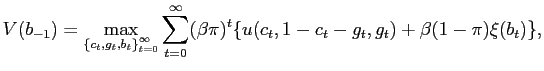
In figure 6 we show the
average value of debt for several degrees of commitment, as
measured by the parameter ![]() .29 We
find that even a relatively small departure from the
full-commitment assumption makes the economy behave very similarly
to the no-commitment case. If at period
.29 We
find that even a relatively small departure from the
full-commitment assumption makes the economy behave very similarly
to the no-commitment case. If at period ![]() the
government holds debt (assets), it accumulates surpluses
(deficits), until the level of zero debt is reached. Hence, the
property that the steady-state level of debt is determined by the
initial conditions is not robust to small deviations from the
full-commitment case.
the
government holds debt (assets), it accumulates surpluses
(deficits), until the level of zero debt is reached. Hence, the
property that the steady-state level of debt is determined by the
initial conditions is not robust to small deviations from the
full-commitment case.
Figure 6: Loose commitment: time pattern of debt
Note: The figure plots the evolution of debt over time, under different values of parameter π. The solid line corresponds to the case of π = .5. We take average across simulations of the histories of the shock ![]() . The initial conditions is b = .16 (roughly 50% of GDP).
. The initial conditions is b = .16 (roughly 50% of GDP).
Data for Figure 6
| Time | π = 0.5 | π = 0.9 |
|---|---|---|
| 1 | 0.15980 | 0.15980 |
| 2 | 0.15859 | 0.16571 |
| 3 | 0.15115 | 0.16133 |
| 4 | 0.14398 | 0.15708 |
| 5 | 0.13753 | 0.15296 |
| 6 | 0.13174 | 0.14897 |
| 7 | 0.12582 | 0.14465 |
| 8 | 0.12027 | 0.14112 |
| 9 | 0.11546 | 0.13748 |
| 10 | 0.11098 | 0.13394 |
| 11 | 0.10609 | 0.13028 |
| 12 | 0.10191 | 0.12674 |
| 13 | 0.09774 | 0.12374 |
| 14 | 0.09349 | 0.12017 |
| 15 | 0.08995 | 0.11714 |
| 16 | 0.08743 | 0.11462 |
| 17 | 0.08405 | 0.11155 |
| 18 | 0.08070 | 0.10856 |
| 19 | 0.07770 | 0.10567 |
| 20 | 0.07459 | 0.10288 |
| 21 | 0.07199 | 0.10038 |
| 22 | 0.06943 | 0.09774 |
| 23 | 0.06759 | 0.09528 |
| 24 | 0.06522 | 0.09295 |
| 25 | 0.06287 | 0.09068 |
| 26 | 0.06097 | 0.08831 |
| 27 | 0.05816 | 0.08599 |
| 28 | 0.05588 | 0.08390 |
| 29 | 0.05375 | 0.08148 |
| 30 | 0.05180 | 0.07936 |
| 31 | 0.05027 | 0.07742 |
| 32 | 0.04859 | 0.07543 |
| 33 | 0.04669 | 0.07365 |
| 34 | 0.04521 | 0.07174 |
| 35 | 0.04374 | 0.07004 |
| 36 | 0.04211 | 0.06828 |
| 37 | 0.04064 | 0.06651 |
| 38 | 0.03927 | 0.06477 |
| 39 | 0.03814 | 0.06323 |
| 40 | 0.03706 | 0.06200 |
| 41 | 0.03586 | 0.06056 |
| 42 | 0.03481 | 0.05913 |
| 43 | 0.03385 | 0.05774 |
| 44 | 0.03275 | 0.05638 |
| 45 | 0.03187 | 0.05506 |
| 46 | 0.03069 | 0.05355 |
| 47 | 0.02954 | 0.05231 |
| 48 | 0.02888 | 0.05100 |
| 49 | 0.02834 | 0.04998 |
| 50 | 0.02730 | 0.04896 |
| 51 | 0.02658 | 0.04800 |
| 52 | 0.02580 | 0.04692 |
| 53 | 0.02513 | 0.04583 |
| 54 | 0.02451 | 0.04471 |
| 55 | 0.02383 | 0.04377 |
| 56 | 0.02278 | 0.04268 |
| 57 | 0.02222 | 0.04178 |
| 58 | 0.02134 | 0.04032 |
| 59 | 0.02074 | 0.03930 |
| 60 | 0.02025 | 0.03831 |
| 61 | 0.01963 | 0.03738 |
| 62 | 0.01902 | 0.03653 |
| 63 | 0.01857 | 0.03567 |
| 64 | 0.01823 | 0.03488 |
| 65 | 0.01781 | 0.03409 |
| 66 | 0.01741 | 0.03344 |
| 67 | 0.01691 | 0.03260 |
| 68 | 0.01637 | 0.03192 |
| 69 | 0.01586 | 0.03109 |
| 70 | 0.01544 | 0.03034 |
| 71 | 0.01501 | 0.02970 |
| 72 | 0.01455 | 0.02900 |
| 73 | 0.01426 | 0.02843 |
| 74 | 0.01381 | 0.02788 |
| 75 | 0.01338 | 0.02726 |
| 76 | 0.01304 | 0.02669 |
| 77 | 0.01282 | 0.02617 |
| 78 | 0.01241 | 0.02561 |
| 79 | 0.01206 | 0.02501 |
| 80 | 0.01157 | 0.02445 |
| 81 | 0.01130 | 0.02394 |
| 82 | 0.01095 | 0.02349 |
| 83 | 0.01072 | 0.02287 |
| 84 | 0.01042 | 0.02240 |
| 85 | 0.01016 | 0.02181 |
| 86 | 0.00999 | 0.02148 |
| 87 | 0.00960 | 0.02115 |
| 88 | 0.00925 | 0.02070 |
| 89 | 0.00904 | 0.02027 |
| 90 | 0.00872 | 0.01978 |
| 91 | 0.00855 | 0.01924 |
| 92 | 0.00833 | 0.01877 |
| 93 | 0.00811 | 0.01830 |
| 94 | 0.00777 | 0.01790 |
| 95 | 0.00752 | 0.01751 |
| 96 | 0.00728 | 0.01697 |
| 97 | 0.00713 | 0.01669 |
| 98 | 0.00693 | 0.01630 |
| 99 | 0.00671 | 0.01591 |
| 100 | 0.00653 | 0.01555 |
| 101 | 0.00632 | 0.01524 |
| 102 | 0.00611 | 0.01492 |
| 103 | 0.00584 | 0.01440 |
| 104 | 0.00564 | 0.01404 |
| 105 | 0.00552 | 0.01375 |
| 106 | 0.00537 | 0.01343 |
| 107 | 0.00521 | 0.01315 |
| 108 | 0.00504 | 0.01284 |
| 109 | 0.00489 | 0.01250 |
| 110 | 0.00473 | 0.01228 |
| 111 | 0.00466 | 0.01196 |
| 112 | 0.00453 | 0.01168 |
| 113 | 0.00442 | 0.01145 |
| 114 | 0.00429 | 0.01131 |
| 115 | 0.00417 | 0.01110 |
| 116 | 0.00406 | 0.01086 |
| 117 | 0.00395 | 0.01069 |
| 118 | 0.00385 | 0.01042 |
| 119 | 0.00371 | 0.01020 |
| 120 | 0.00362 | 0.00997 |
| 121 | 0.00350 | 0.00962 |
| 122 | 0.00338 | 0.00945 |
| 123 | 0.00329 | 0.00925 |
| 124 | 0.00320 | 0.00902 |
| 125 | 0.00312 | 0.00881 |
| 126 | 0.00301 | 0.00857 |
| 127 | 0.00290 | 0.00844 |
| 128 | 0.00283 | 0.00825 |
| 129 | 0.00276 | 0.00807 |
| 130 | 0.00268 | 0.00789 |
| 131 | 0.00261 | 0.00770 |
| 132 | 0.00252 | 0.00752 |
| 133 | 0.00245 | 0.00742 |
| 134 | 0.00240 | 0.00725 |
| 135 | 0.00234 | 0.00704 |
| 136 | 0.00228 | 0.00686 |
| 137 | 0.00223 | 0.00666 |
| 138 | 0.00216 | 0.00649 |
| 139 | 0.00207 | 0.00633 |
| 140 | 0.00200 | 0.00616 |
| 141 | 0.00194 | 0.00605 |
| 142 | 0.00187 | 0.00601 |
| 143 | 0.00181 | 0.00584 |
| 144 | 0.00175 | 0.00569 |
| 145 | 0.00171 | 0.00557 |
| 146 | 0.00168 | 0.00544 |
| 147 | 0.00166 | 0.00531 |
| 148 | 0.00159 | 0.00519 |
| 149 | 0.00155 | 0.00509 |
| 150 | 0.00149 | 0.00497 |
| 151 | 0.00147 | 0.00488 |
| 152 | 0.00142 | 0.00476 |
| 153 | 0.00138 | 0.00470 |
| 154 | 0.00132 | 0.00455 |
| 155 | 0.00128 | 0.00447 |
| 156 | 0.00125 | 0.00436 |
| 157 | 0.00120 | 0.00428 |
| 158 | 0.00117 | 0.00421 |
| 159 | 0.00113 | 0.00416 |
| 160 | 0.00111 | 0.00407 |
| 161 | 0.00108 | 0.00396 |
| 162 | 0.00104 | 0.00386 |
| 163 | 0.00102 | 0.00377 |
| 164 | 0.00099 | 0.00367 |
| 165 | 0.00096 | 0.00358 |
| 166 | 0.00094 | 0.00351 |
| 167 | 0.00093 | 0.00345 |
| 168 | 0.00090 | 0.00339 |
| 169 | 0.00088 | 0.00331 |
| 170 | 0.00086 | 0.00321 |
| 171 | 0.00085 | 0.00313 |
| 172 | 0.00083 | 0.00306 |
| 173 | 0.00081 | 0.00300 |
| 174 | 0.00078 | 0.00295 |
| 175 | 0.00076 | 0.00288 |
| 176 | 0.00073 | 0.00282 |
| 177 | 0.00070 | 0.00276 |
| 178 | 0.00068 | 0.00273 |
| 179 | 0.00066 | 0.00265 |
| 180 | 0.00065 | 0.00258 |
| 181 | 0.00063 | 0.00253 |
| 182 | 0.00062 | 0.00247 |
| 183 | 0.00060 | 0.00241 |
| 184 | 0.00058 | 0.00235 |
| 185 | 0.00057 | 0.00229 |
| 186 | 0.00056 | 0.00224 |
| 187 | 0.00054 | 0.00219 |
| 188 | 0.00052 | 0.00214 |
| 189 | 0.00050 | 0.00209 |
| 190 | 0.00049 | 0.00201 |
| 191 | 0.00048 | 0.00197 |
| 192 | 0.00047 | 0.00193 |
| 193 | 0.00045 | 0.00191 |
| 194 | 0.00044 | 0.00187 |
| 195 | 0.00042 | 0.00183 |
| 196 | 0.00041 | 0.00179 |
| 197 | 0.00039 | 0.00174 |
| 198 | 0.00038 | 0.00170 |
| 199 | 0.00038 | 0.00166 |
| 200 | 0.00037 | 0.00163 |
Table 1: Average long-run allocations under loose commitment
| Variable | COM | π = .75 | No COM |
|---|---|---|---|
| y | 0.32 | 0.32 | 0.32 |
| b / y | 0.54 | 0.00 | 0.00 |
| g / y | 0.23 | 0.23 | 0.23 |
| c / y | 0.77 | 0.77 | 0.77 |
| τ | 0.25 | 0.23 | 0.23 |
In table 1,
we show long-run average allocations with a degree of commitment of
![]() , together with the full-commitment
and no-commitment cases.30 Unless there is full-commitment, the
debt/GDP ratio is zero, due to the reasons explained above. All the
other ratios are substantially unchanged, apart from a small
reduction in taxes. In this type of models, the steady-state
interest rate is not affected by the outstanding level of
debt.31 As a consequence, a different level
of debt only affects the base to which the interest rate is
applied. This explains why lower debt implies lower taxation, and
only slightly affects the other allocations. table
, together with the full-commitment
and no-commitment cases.30 Unless there is full-commitment, the
debt/GDP ratio is zero, due to the reasons explained above. All the
other ratios are substantially unchanged, apart from a small
reduction in taxes. In this type of models, the steady-state
interest rate is not affected by the outstanding level of
debt.31 As a consequence, a different level
of debt only affects the base to which the interest rate is
applied. This explains why lower debt implies lower taxation, and
only slightly affects the other allocations. table
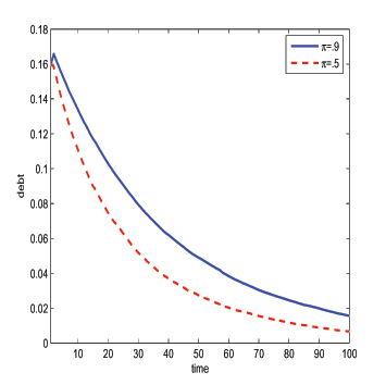
To gain a deeper understanding of the transition dynamics, it is
useful to look at figure 7. Here
we consider a particular realization of the shocks
![]() , where a
reoptimization occurs every 4 periods, independently of the
probability
, where a
reoptimization occurs every 4 periods, independently of the
probability ![]() .
.
Figure 7: Loose commitment: reoptimization every 4 periods
Note: The figure plots the evolution of debt over time, in the particular history of the shock ![]() such that a reoptimization occurs every four periods. The solid line corresponds to the case of π = .9, while the dashed line corresponds to the case of π = .5. The initial condition is b = .16 (roughly 50% of GDP).
such that a reoptimization occurs every four periods. The solid line corresponds to the case of π = .9, while the dashed line corresponds to the case of π = .5. The initial condition is b = .16 (roughly 50% of GDP).
Data for Figure 7
| Time | π = 0.5 | π = 0.9 |
|---|---|---|
| 1 | 0.1598 | 0.1598 |
| 2 | 0.1586 | 0.1621 |
| 3 | 0.1448 | 0.1526 |
| 4 | 0.1321 | 0.1436 |
| 5 | 0.1203 | 0.1350 |
| 6 | 0.1212 | 0.1384 |
| 7 | 0.1103 | 0.1302 |
| 8 | 0.1004 | 0.1223 |
| 9 | 0.0913 | 0.1149 |
| 10 | 0.0928 | 0.1188 |
| 11 | 0.0844 | 0.1116 |
| 12 | 0.0767 | 0.1048 |
| 13 | 0.0697 | 0.0984 |
| 14 | 0.0712 | 0.1024 |
| 15 | 0.0647 | 0.0961 |
| 16 | 0.0588 | 0.0903 |
| 17 | 0.0534 | 0.0847 |
| 18 | 0.0548 | 0.0885 |
| 19 | 0.0498 | 0.0831 |
| 20 | 0.0453 | 0.0780 |
| 21 | 0.0411 | 0.0732 |
| 22 | 0.0423 | 0.0768 |
| 23 | 0.0384 | 0.0721 |
| 24 | 0.0349 | 0.0676 |
| 25 | 0.0317 | 0.0635 |
| 26 | 0.0327 | 0.0668 |
| 27 | 0.0297 | 0.0627 |
| 28 | 0.0270 | 0.0588 |
| 29 | 0.0245 | 0.0552 |
| 30 | 0.0253 | 0.0582 |
| 31 | 0.0230 | 0.0546 |
| 32 | 0.0209 | 0.0512 |
| 33 | 0.0190 | 0.0481 |
| 34 | 0.0196 | 0.0508 |
| 35 | 0.0179 | 0.0477 |
| 36 | 0.0162 | 0.0447 |
| 37 | 0.0147 | 0.0420 |
| 38 | 0.0152 | 0.0444 |
| 39 | 0.0139 | 0.0417 |
| 40 | 0.0126 | 0.0391 |
| 41 | 0.0114 | 0.0367 |
| 42 | 0.0118 | 0.0389 |
| 43 | 0.0108 | 0.0365 |
| 44 | 0.0098 | 0.0343 |
| 45 | 0.0089 | 0.0321 |
| 46 | 0.0092 | 0.0341 |
| 47 | 0.0084 | 0.0320 |
| 48 | 0.0076 | 0.0300 |
| 49 | 0.0069 | 0.0282 |
| 50 | 0.0072 | 0.0300 |
| 51 | 0.0065 | 0.0281 |
| 52 | 0.0059 | 0.0264 |
| 53 | 0.0054 | 0.0247 |
| 54 | 0.0056 | 0.0263 |
| 55 | 0.0051 | 0.0247 |
| 56 | 0.0046 | 0.0232 |
| 57 | 0.0042 | 0.0217 |
| 58 | 0.0043 | 0.0232 |
| 59 | 0.0039 | 0.0217 |
| 60 | 0.0036 | 0.0204 |
| 61 | 0.0032 | 0.0191 |
| 62 | 0.0034 | 0.0204 |
| 63 | 0.0031 | 0.0191 |
| 64 | 0.0028 | 0.0179 |
| 65 | 0.0025 | 0.0168 |
| 66 | 0.0026 | 0.0179 |
| 67 | 0.0024 | 0.0168 |
| 68 | 0.0022 | 0.0158 |
| 69 | 0.0020 | 0.0148 |
| 70 | 0.0020 | 0.0158 |
| 71 | 0.0019 | 0.0148 |
| 72 | 0.0017 | 0.0139 |
| 73 | 0.0015 | 0.0131 |
| 74 | 0.0016 | 0.0139 |
| 75 | 0.0014 | 0.0131 |
| 76 | 0.0013 | 0.0123 |
| 77 | 0.0012 | 0.0115 |
| 78 | 0.0012 | 0.0123 |
| 79 | 0.0011 | 0.0115 |
| 80 | 0.0010 | 0.0108 |
| 81 | 0.0009 | 0.0101 |
| 82 | 0.0010 | 0.0108 |
| 83 | 0.0009 | 0.0102 |
| 84 | 0.0008 | 0.0095 |
| 85 | 0.0007 | 0.0090 |
| 86 | 0.0007 | 0.0096 |
| 87 | 0.0007 | 0.0090 |
| 88 | 0.0006 | 0.0084 |
| 89 | 0.0006 | 0.0079 |
| 90 | 0.0006 | 0.0084 |
| 91 | 0.0005 | 0.0079 |
| 92 | 0.0005 | 0.0074 |
| 93 | 0.0004 | 0.0070 |
| 94 | 0.0005 | 0.0075 |
| 95 | 0.0004 | 0.0070 |
| 96 | 0.0004 | 0.0066 |
| 97 | 0.0003 | 0.0062 |
| 98 | 0.0004 | 0.0066 |
| 99 | 0.0003 | 0.0062 |
| 100 | 0.0003 | 0.0058 |
Interestingly, in the loose commitment framework debt is
increased when a reoptimization occurs and past promises are not
kept. On the other hand, debt is decreased when promises are
fulfilled. This is in contrast with the no-commitment solution,
where debt is always reduced. This occurs because in the
no-commitment solution the planner knows that he can conveniently
affect the interest rate only if debt is reduced. In the loose
commitment setting this is no longer true. With probability
![]() the planner will be replaced, and
promises will not be kept. In that case, the level of debt is key
to determine the policy of the successor and thus the interest
rate. But with probability
the planner will be replaced, and
promises will not be kept. In that case, the level of debt is key
to determine the policy of the successor and thus the interest
rate. But with probability ![]() , promises will
be fulfilled, and such promises will determine the interest rate
independently of the level of debt. In a loose commitment
setting, the planner can thus afford to increase debt when
reoptimizing, and conveniently manipulate the interest rate, as
long as he promises to reduce debt if he stays in office in the
following periods. Finally, if
, promises will
be fulfilled, and such promises will determine the interest rate
independently of the level of debt. In a loose commitment
setting, the planner can thus afford to increase debt when
reoptimizing, and conveniently manipulate the interest rate, as
long as he promises to reduce debt if he stays in office in the
following periods. Finally, if ![]() is near zero
debt is always reduced, no matter whether promises are kept or not.
In that case, debt is reduced at a higher pace when promises are
kept.
is near zero
debt is always reduced, no matter whether promises are kept or not.
In that case, debt is reduced at a higher pace when promises are
kept.
To summarize, in our loose commitment setting, we find that unless the government has full-commitment, debt goes to zero in the long-run and that debt is reduced mainly in the periods over which the government has commitment. This is saying that the behavior of the economy resembles the one that would prevail under no-commitment. Moreover, our considerations about the transition dynamics suggests that the simple possibility that in a future period a reoptimization will occur is enough to make it optimal to reach the zero level of debt.
5 Political disagreement
In this section, we extend our analysis to take into account political disagreement among successive planners alternating in office. There are two reasons why we believe this case is interesting.
First, this is a case where the assumption of imperfect commitment is natural. In the presence of political turnover, the party currently in office cannot make credible commitments about the choices of a successor, who in general has different objectives. As explained in the previous section, imperfect commitment, per se, drives debt to zero.32
Second, as discussed in Alesina and Tabellini (1990), the presence of political disagreement and political uncertainty provides an incentive to accumulate an excessive level of debt with respect to the standard (Ramsey) case. In particular, they show that disagreement on the composition of the public good and more frequent political turnovers lead to a higher steady state level of debt.
The literature dealing with dynamic models of political turnover has typically used frameworks where the policymakers' commitment assumption is irrelevant to determine private agents' choices. For example, this happens whenever the current choices of the agents (e.g. their savings/consumptions) do not depend on the expectations about future policy choices (e.g., future taxes, public expenditure, etc.).
Our contributions with respect to this literature are the following. First, we consider a framework where the time-inconsistency of policy choices do play a role in the strategic interactions between private agents and policymakers. In our case, the time-inconsistency problem arises because of the governments' incentives to manipulate the interest rate once the amount of private savings is given. Second, we combine imperfect commitment with political disagreement into a unique framework. We first solve the problem assuming that governments cannot make credible commitments about their future actions, no matter whether they are reappointed in office or not. In such circumstances, the probability of re-election is totally unrelated to the probability of being committed in the future. Moreover, we also consider the case that governments can commit for the case they are reappointed, but cannot commit on behalf of their successors. By doing so, we are able to distinguish and quantify the effects of imperfect commitment and political disagreement, which in principle would seem to drive debt in opposite directions. Finally, it allows to measure the welfare gains from commitment in the presence of political disagreement.
Consider that two political parties (![]() and
and
![]() ) have equal preferences regarding private
consumption and leisure. However, both parties disagree on how to
allocate the public expenditure
) have equal preferences regarding private
consumption and leisure. However, both parties disagree on how to
allocate the public expenditure ![]() . More formally, we
assume that when a given party is in power its period utility
. More formally, we
assume that when a given party is in power its period utility
![]() is given by equation (13). However, if
the party is not in power, and therefore it is not deciding on the
allocation of the public expenditure, then the period utility
is given by equation (13). However, if
the party is not in power, and therefore it is not deciding on the
allocation of the public expenditure, then the period utility
![]() is given by
is given by
![$\displaystyle \tilde{u}(c_{t},l_{t},g_{t})=(1-\phi_{g})\left[ \phi_{c}\frac{(c_{t} )^{1-\sigma_{c}}-1}{1-\sigma_{c}}+(1-\phi_{c})\frac{(x_{t})^{1-\sigma_{x}} -1}{1-\sigma_{x}}\right] +\phi_{g}\alpha\frac{(g_{t})^{1-\sigma_{g}} -1}{1-\sigma_{g}}$](img136.gif)
|
(16) |
where the parameter
![]() measures the degree of
disagreement between the two parties. Due to political disagreement
the period utility of the party that is not in power is lower. The
higher is
measures the degree of
disagreement between the two parties. Due to political disagreement
the period utility of the party that is not in power is lower. The
higher is ![]() , the lower is the disagreement
between both parties. A value of
, the lower is the disagreement
between both parties. A value of ![]() represents
the limiting case of no disagreement. The political disagreement
captured by
represents
the limiting case of no disagreement. The political disagreement
captured by ![]() can be due to several reasons.
Political parties may attach more weight to different social
groups, or regions inside the country. Hence, parties may disagree
on the geographical location of certain public goods, and
consequently which social groups can benefit more from those goods.
Different parties may also disagree on the composition of public
expenditure, or which private contractors should provide the public
goods. In the appendix, we provide specific examples where
disagreement gives rise to the preferences that we have specified
in (13) and
(16).
can be due to several reasons.
Political parties may attach more weight to different social
groups, or regions inside the country. Hence, parties may disagree
on the geographical location of certain public goods, and
consequently which social groups can benefit more from those goods.
Different parties may also disagree on the composition of public
expenditure, or which private contractors should provide the public
goods. In the appendix, we provide specific examples where
disagreement gives rise to the preferences that we have specified
in (13) and
(16).
It can be shown that the problem of a government of type
![]() , at the beginning of its tenure, can
be written as
, at the beginning of its tenure, can
be written as
|
(17) |
subject to the sequence of constraint (14) for
![]() .
.
The previous formulation is similar to the one of problem
(15). The main
difference is that, when a reoptimization occurs, choices are taken
by another party that will allocate the public expenditure
![]() in a different way. As a consequence, in
the objective function of party
in a different way. As a consequence, in
the objective function of party ![]() , the function
, the function
![]() is the lifetime
utility that party
is the lifetime
utility that party ![]() obtains if the other party
is elected at
obtains if the other party
is elected at ![]() .
.
The utility received by each party depends on whether they are
in power or not. Since the problem faced by the two political
parties is fully symmetric, in a given state of the world they will
always choose the same level of debt, private consumption, leisure,
taxes and public expenditure.33 This symmetry allows us to define
the lifetime utility derived by a party ![]() when the
other party is in charge
when the
other party is in charge
![]() as
as
![$\displaystyle \underset{}{\xi(b_{-1})=}\sum_{t=0}^{\infty}\left( \beta\pi\right) ^{t}\left[ \tilde{u}(c^{*}_{t},1-c^{*}_{t}-g^{*}_{t}, g^{*}_{t}) +\beta\left( 1-\pi\right) V( b^{*}_{t+1}) \right]$](img151.gif)
|
(18) |
where stars denote variables evaluated with the policy functions
solving problem (17).
Since the other party is in charge, allocations are evaluated
according to ![]() instead of
instead of ![]() .
The value function
.
The value function ![]() is present because
party
is present because
party ![]() may regain power, and obtain utility
may regain power, and obtain utility
![]() as defined in (17).
In the case there is no disagreement (
as defined in (17).
In the case there is no disagreement (![]() ), we
have that
), we
have that
![]() .
.
Definition 1 specifies our concept of equilibrium, which we restrict to be within the class of Markov equilibria.
- Given
 and
and  , the
allocation
, the
allocation
 solves
problem (17);
solves
problem (17); - The value function
 is described by
Eq.(18)
and
is described by
Eq.(18)
and  is the maximum of problem (17);
 - The policy function of consumption
 solving problem (17)
is such that
solving problem (17)
is such that
 .
.
The first part of the definition is a simple optimality
requirement. The second part states that the functions ![]() and
and ![]() need to be consistent between
themselves. The third part of the definition, states that the
functions the future government is expected to implement are
optimal. Since the current and future governments face the same
problem, the functions that the current government and future
governments implement are equal. In particular, it is worth
recalling that the public good provided only changes in nature, but
not in level. Nevertheless, as in the loose commitment case of
section 4,
when a new government is elected the Lagrange multiplier
(
need to be consistent between
themselves. The third part of the definition, states that the
functions the future government is expected to implement are
optimal. Since the current and future governments face the same
problem, the functions that the current government and future
governments implement are equal. In particular, it is worth
recalling that the public good provided only changes in nature, but
not in level. Nevertheless, as in the loose commitment case of
section 4,
when a new government is elected the Lagrange multiplier
(![]() ) is set to zero.
) is set to zero.
As explained in section 4, ![]() and the value function
and the value function ![]() are
unknown and need to be found as a solution of a fixed point
problem. In the current case, however, the fact that
are
unknown and need to be found as a solution of a fixed point
problem. In the current case, however, the fact that ![]() and
and ![]() are not equal does not allow us
to apply envelope results as can be done in absence of
disagreement.
are not equal does not allow us
to apply envelope results as can be done in absence of
disagreement.
Our formulation (17)
allows to study all the combinations of degree of commitment and
political disagreement. For example, if ![]() and
and
![]() we have full commitment and no
disagreement among planners, as in the standard Ramsey formulation
of section 2.1. On the other
extreme, when
we have full commitment and no
disagreement among planners, as in the standard Ramsey formulation
of section 2.1. On the other
extreme, when ![]() and
and ![]() we
have political disagreement with no-commitment. By changing the
values of the parameters
we
have political disagreement with no-commitment. By changing the
values of the parameters ![]() and
and ![]() , we are therefore able to disentangle the effects of
these two sources of inefficiency.
, we are therefore able to disentangle the effects of
these two sources of inefficiency.
5.1 The effects of political disagreement and no-commitment
We start by considering the effect of political disagreement,
abstracting from commitment issues. In other words, as in Alesina and Tabellini (1990), we keep the extreme assumption that
governments can never commit, no matter if they are re-elected or
not, and act with full discretion. In this case, the parameter
![]() is unrelated to the degree of commitment
and only measures the probability of being reelected.
is unrelated to the degree of commitment
and only measures the probability of being reelected.
Table 2 shows the
long-run level of debt for different values of ![]() and
and ![]() . First, once there is political
disagreement between successive planners, debt converges to a
positive level in the long-run. Second, a higher degree of
disagreement (i.e. lower
. First, once there is political
disagreement between successive planners, debt converges to a
positive level in the long-run. Second, a higher degree of
disagreement (i.e. lower ![]() ) and more frequent
turnover (lower value of
) and more frequent
turnover (lower value of ![]() ), imply a higher level of
debt. However, while the effects of different degrees of
disagreement are relevant, those of the frequency of turnover seems
quantitatively less important. Indeed, for all the values of
), imply a higher level of
debt. However, while the effects of different degrees of
disagreement are relevant, those of the frequency of turnover seems
quantitatively less important. Indeed, for all the values of
![]() reported, the difference on the level
of debt between having
reported, the difference on the level
of debt between having ![]() and
and ![]() is less than 10% of GDP.
is less than 10% of GDP.
Table 2: Long-run debt (% of GDP) with political disagreement and no-commitment
α | π = 1 | π = 0.9 | π = 0.75 | π = 0.5 | π = 0.25 | π = 0 |
|---|---|---|---|---|---|---|
1 | - | 0.0 | 0.0 | 0.0 | 0.0 | 0.0 |
0.99 | - | 10.9 | 13.0 | 13.9 | 14.2 | 14.4 |
0.98 | - | 17.8 | 20.9 | 22.3 | 22.8 | 23.0 |
0.97 | - | 23.1 | 27.0 | 28.6 | 29.2 | 29.6 |
0.96 | - | 27.4 | 31.9 | 33.9 | 34.6 | 34.9 |
0.95 | - | 31.2 | 36.2 | 38.3 | 39.1 | 39.5 |
Note: The table reports the long-run level of debt, for different degree of disagreement (α) and frequency of turnover (π). Governments do not have commitment, regardless of the probability (π).
5.2 The effects of political disagreement with commitment
We now investigate the case where a government does commit over its tenure, but cannot commit on behalf of its successors. Besides being a more realistic depiction of reality, there are three main reasons to investigate this case. First, from a static point of view, to see the implications of political disagreement without removing completely the commitment assumption. Second, from a dynamic perspective, allowing for commitment over the tenure in the presence of political disagreement generates volatility in the variables as a consequence of political cycles, even in a fully symmetric model as ours. Indeed, because of the possibility to commit, choices differ depending on whether the government is new in office or not. Third, we can investigate the gains from commitment in a world characterized by political disagreement.
We should first note that, in this context, a higher political
turnover also necessarily implies a lower degree of commitment. The
lower is the probability of being re-elected, the shorter is the
horizon over which the government is expected to commit. In other
words, there are now two effects related to the parameter
![]() . A higher
. A higher ![]() first
implies less frequent turnover which leads, ceteris paribus
to slightly lower debt, according to our analysis in section
5.1.
But it also means a higher degree of commitment, as shown in
section 4.
Exploring the composite effects of these two forces seems therefore
worthwhile.
first
implies less frequent turnover which leads, ceteris paribus
to slightly lower debt, according to our analysis in section
5.1.
But it also means a higher degree of commitment, as shown in
section 4.
Exploring the composite effects of these two forces seems therefore
worthwhile.
In table 3, we show the
average long-run level of debt in the case of political
disagreement and commitment over the tenure. As in the previous
case, the level of debt is considerably increasing in the degree of
disagreement. The effects of ![]() on debt are less
clear. For reasonable values of
on debt are less
clear. For reasonable values of ![]() debt does not
change substantially.34 In addition, as
debt does not
change substantially.34 In addition, as ![]() changes, debt changes non-monotonically. Indeed, as can
be seen comparing the second and third column, increasing
changes, debt changes non-monotonically. Indeed, as can
be seen comparing the second and third column, increasing
![]() from .75 to .9, as opposed to the
previous case, may lead to an increase in the debt/GDP ratio. This
is because of the following. A higher
from .75 to .9, as opposed to the
previous case, may lead to an increase in the debt/GDP ratio. This
is because of the following. A higher ![]() means a
longer tenure on average. On the one hand, the commitment horizon
is longer. This means that debt can be increased by more when a
reoptimization occurs. On the other hand, it is less likely that
the other party comes into power, so the incentives to accumulate
debt are smaller. The composite effect of changing
means a
longer tenure on average. On the one hand, the commitment horizon
is longer. This means that debt can be increased by more when a
reoptimization occurs. On the other hand, it is less likely that
the other party comes into power, so the incentives to accumulate
debt are smaller. The composite effect of changing ![]() depends on the relative strength of these two forces,
which are difficult to disentangle. Finally, the effects of a
marginal change in the frequency of political turnover depends on
the degree of disagreement. This suggests that, from an empirical
point of view, it is important to consider the interactions among
the two forces when testing the relationship between debt policies
and political instability.
depends on the relative strength of these two forces,
which are difficult to disentangle. Finally, the effects of a
marginal change in the frequency of political turnover depends on
the degree of disagreement. This suggests that, from an empirical
point of view, it is important to consider the interactions among
the two forces when testing the relationship between debt policies
and political instability.
Table 3: Long-run debt (% of GDP) with political disagreement and commitment over the tenure
α |
π = 1 |
π = 0.9 |
π = 0.75 |
π = 0.5 |
π = 0.25 |
π = 0 |
|---|---|---|---|---|---|---|
1 |
- |
0.0 |
0.0 |
0.0 |
0.0 |
0.0 |
0.99 |
- |
3.6 |
3.6 |
4.6 |
6.9 |
14.4 |
0.98 |
- |
7.0 |
7.0 |
8.9 |
12.7 |
23.0 |
0.97 |
- |
10.4 |
10.3 |
12.9 |
17.6 |
29.6 |
0.96 |
- |
13.8 |
13.5 |
16.6 |
21.8 |
34.9 |
0.95 |
- |
17.1 |
16.7 |
20.1 |
25.5 |
39.5 |
Note: The table reports the average long-run level of debt for different degree of disagreement (α) and frequency of turnover (π). Averages are taken across realizations of the shock sT, where T = 1000.
By comparing table 2 and table 3, we can also see that the long-run level of debt is lower when there is commitment within the tenure than if governments cannot commit. As mentioned in the loose commitment setting of section 4, debt is reduced during the commitment periods and increased whenever past plans are abandoned. In the present context, when governments can commit over their tenure, debt is lower on average because of the longer commitment horizon of alternating governments.
To summarize, according to our model, differences in the frequency of political turnover cannot account for the differences in the level of debt across countries and over time. There are mainly two reasons for this result. First, from a qualitative point of view, the relationship between frequency of turnover and the level of debt seems unclear. This crucially depends on the relative importance of the opposite effects of having a longer tenure versus those of having a longer commitment horizon. Second, from a quantitative point of view, such effects seems of minor importance. The predictions of the model suggest that it is the different degree of polarization among the political forces, rather than the frequency of political turnover and the degree of commitment, what really matters in explaining the differences in the debt level across countries and over time.
5.3 Relationship with the empirical evidence
There is a large body of empirical studies about the effects of political polarization and frequency of turnover on deficits and debt accumulation. However, in most of these studies, polarization and turnover are not analyzed together, since they are usually considered as alternative proxies of political instability.
There are many studies analyzing the effects of political polarization on public debt and deficits. Different works have measured polarization in different ways, but it is generally found that a larger degree of polarization increases debt. Roubini and Sachs (1989) find that coalition governments (interpreted as polarization) are more likely to run deficits.35 Volkerink and de Haan (2001) and Huber et al. (2003) find that the fragmentation of governments (in terms of size or political ideology) is a source for relatively higher deficits. Alt and Lassen (2006) find that fiscal transparency and less polarization reduce debt. Woo (2003) finds that countries with high polarization, measured as income inequality, have bigger fiscal deficits.
There is also a large empirical literature examining the effects of the average tenure or the re-election probability. In this case, however, results are controversial. Alt and Lassen (2006), in contradiction with the theory, find that shorter tenures reduce debt. Skilling and Zeckhauser (2002) also find that political competition decreases debt. Lambertini (2004) and Franzese (2001) find that the incumbent's probability of being voted out of office can not explain budget deficits. Grilli et al. (1991) find mixed results regarding the effects of the average tenure. de Haan and Sturm (1994) find that the frequency of government changes is positively correlated to budget deficits.
The overview of the empirical literature shows that there is some consensus that polarization is translated into more debt or deficits. In contrast, the findings on the re-election probability are quite mixed. Our paper can help understand these results. We find that both polarization and the probability of election matters, but the effect of the second variable is small. Different degrees of commitment and small changes in the economic structure among countries may blur the effects of the re-election probability. On the other hand, our model suggests that the effects of polarization are quite strong and easy to detect, as the data confirms. Most importantly, our analysis suggests the importance to consider both the degree of political polarization and the frequency of turnover in the empirical tests of the relationship between debt and political instability.
5.4 Welfare implications
For all the settings analyzed in the previous sections, we
computed the consumption equivalent variation from the second-best
full-commitment and no-disagreement case. In figure 8, we show the
welfare costs of imperfect commitment. Moving from full-commitment
(![]() ) to no-commitment (
) to no-commitment (![]() ), the implied loss is equivalent to a per-period
reduction in consumption of 0.07%. This means that while the degree
of commitment has a big impact on the level of debt, it has less
striking welfare implications. The level of debt only affects
allocations because of the interest rate payments. In a model where
the government can default on its outstanding debt these effects
are likely to be bigger. Analyzing such case is certainly
interesting, but is out of the scope of the present analysis. Our
work should serve as a reference for countries with small risk of
default and which can easily refinance their debt.
), the implied loss is equivalent to a per-period
reduction in consumption of 0.07%. This means that while the degree
of commitment has a big impact on the level of debt, it has less
striking welfare implications. The level of debt only affects
allocations because of the interest rate payments. In a model where
the government can default on its outstanding debt these effects
are likely to be bigger. Analyzing such case is certainly
interesting, but is out of the scope of the present analysis. Our
work should serve as a reference for countries with small risk of
default and which can easily refinance their debt.
Figure 8: The welfare costs of losing commitment
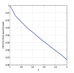
Note: The figure plots the welfare losses from reducing commitment (as measured by π) in a world without political disagreement, expressed in percentage consumption-equivalent variation (CEV) from the benchmark case of full-commitment.
Data for Figure 8
Time | Welfare |
|---|---|
1.00 | 0.00 |
0.75 | -0.03 |
0.50 | -0.04 |
0.25 | -0.06 |
0.00 | -0.07 |
We now consider the welfare implications in a world with political disagreement. In this context, building commitment is not necessarily welfare improving. Commitment is used to pursue partisan objectives, and it can thus be detrimental for agents having different preferences from the party in office. In what follows, we use as measure of social welfare the average of the lifetime utility of the two types of agents, and then compute the consumption equivalent variation from the second-best solution.36
First, we analyze the welfare implications of less frequent
political turnover (i.e. higher ![]() ). For this
purpose, figure 9 shows the
consumption equivalent variation for different values of
). For this
purpose, figure 9 shows the
consumption equivalent variation for different values of
![]() , for a given degree of disagreement (
, for a given degree of disagreement (![]() ). The dashed line refers to the
case where governments cannot commit, while the continuous line
indicates the case where governments commit over their tenures.
When governments do not have commitment over the tenure, welfare is
almost constant in
). The dashed line refers to the
case where governments cannot commit, while the continuous line
indicates the case where governments commit over their tenures.
When governments do not have commitment over the tenure, welfare is
almost constant in ![]() , which says that the
frequency of turnover, per se, is quantitatively irrelevant
in terms of welfare. However, when governments have commitment over
their tenure, the lower is the frequency of turnover the higher is
welfare. In this case, a higher
, which says that the
frequency of turnover, per se, is quantitatively irrelevant
in terms of welfare. However, when governments have commitment over
their tenure, the lower is the frequency of turnover the higher is
welfare. In this case, a higher ![]() means not only
less frequent turnover but also a longer commitment horizon. This
last component seems therefore the one with more important welfare
implications. In figure 10, we
analyze the welfare consequences of increasing
means not only
less frequent turnover but also a longer commitment horizon. This
last component seems therefore the one with more important welfare
implications. In figure 10, we
analyze the welfare consequences of increasing ![]() in a world where governments have commitment over the
tenure and there is political disagreement. The figure plots the
welfare gains achieved by increasing
in a world where governments have commitment over the
tenure and there is political disagreement. The figure plots the
welfare gains achieved by increasing ![]() from zero
to another value. We find that the higher is disagreement (i.e. the
lower is
from zero
to another value. We find that the higher is disagreement (i.e. the
lower is ![]() ) the lower are the welfare gains for
an increase in
) the lower are the welfare gains for
an increase in ![]() . This result is interesting
since it suggests that building commitment is less important in a
country with more polarization among political parties.
. This result is interesting
since it suggests that building commitment is less important in a
country with more polarization among political parties.
Figure 9: The welfare costs of political turnover (α = .95)
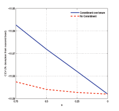
Note: The figure plots the welfare gains from less frequent turnover (as measured by π) in a world with political disagreement (α = .95). The continous line refers to the case where governments can commit over their tenure, while the dashed line refers to the case where there is not commitment over the tenure (regardless of π). Values are expressed in percentage consumption-equivalent variation (CEV) from the benchmark case of full-commitment and no-disagreement.
Data for Figure 9
Time | Welfare 1 | Welfare 2 |
|---|---|---|
0.75 | -11.8826 | -11.8573 |
0.50 | -11.8859 | -11.8681 |
0.25 | -11.8872 | -11.8780 |
0.00 | -11.8880 | -11.8880 |
Figure 10: The welfare gains of less frequent political turnover
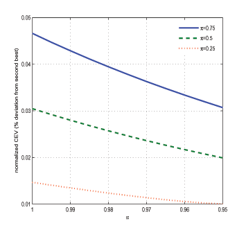
Note: The figure plots the consequences of political disagreement (measured by α) to the welfare gains of increasing π. We first computed welfare for each π measured as percentage consumption-equivalent variation (CEV) from the benchmark case of full-commitment and no-disagreement. In the figure, each line plots the welfare differences from π = 0 to another level of π.
Data for Figure 10
α | Welfare 1 | Welfare 2 | Welfare 3 |
|---|---|---|---|
1.000 | 0.0147 | 0.0305 | 0.0466 |
0.995 | 0.0141 | 0.0292 | 0.0447 |
0.990 | 0.0135 | 0.0280 | 0.0429 |
0.985 | 0.0129 | 0.0268 | 0.0411 |
0.980 | 0.0124 | 0.0257 | 0.0394 |
0.975 | 0.0119 | 0.0246 | 0.0378 |
0.970 | 0.0114 | 0.0236 | 0.0363 |
0.965 | 0.0109 | 0.0226 | 0.0348 |
0.960 | 0.0106 | 0.0217 | 0.0334 |
0.955 | 0.0102 | 0.0208 | 0.0320 |
0.950 | 0.0100 | 0.0199 | 0.0307 |
Second, in a world characterized by political disagreement, we
compute the welfare implications of having commitment over the
tenure. For this purpose, in figure 11, we show the
difference in welfare (in consumption equivalent variation from
second-best) between having commitment over the tenure and not
having commitment. We plot such differences for several values of
![]() and for values of
and for values of ![]() and
and ![]() .37 We observe that
the difference in welfare is positive. Interestingly this is saying
that having governments committing over their tenures is welfare
improving also in a world with political disagreement. We also
notice that such gains from commitment are decreasing in
.37 We observe that
the difference in welfare is positive. Interestingly this is saying
that having governments committing over their tenures is welfare
improving also in a world with political disagreement. We also
notice that such gains from commitment are decreasing in
![]() . This suggests once more that
building commitment is less important the higher is the degree of
polarization (i.e. the lower is
. This suggests once more that
building commitment is less important the higher is the degree of
polarization (i.e. the lower is ![]() ).
).
Figure 11: The welfare gains from Commitment in the presence of political disagreement
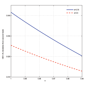
Note: The figure plots, for several degrees of disagreement (measured by α) the difference in welfare (in percentage consumption-equivalent variation (CEV) from second-best), between the case where governments have commitment over their tenure and the case where there is not commitment over the tenure (regardless of π).
Data for Figure 11
α | Welfare 1 | Welfare 2 |
|---|---|---|
1.000 | 0.03047 | 0.04661 |
0.995 | 0.02901 | 0.04420 |
0.990 | 0.02761 | 0.04187 |
0.985 | 0.02624 | 0.03960 |
0.980 | 0.02492 | 0.03739 |
0.975 | 0.02364 | 0.03524 |
0.970 | 0.02241 | 0.03315 |
0.965 | 0.02121 | 0.03111 |
0.960 | 0.02005 | 0.02912 |
0.955 | 0.01892 | 0.02718 |
0.950 | 0.01783 | 0.02528 |
In a world with political disagreement, the fact that a government has commitment may be detrimental for agents having different preferences from the policymaker. This is shown in figure 12, where we compare the welfare implications of commitment depending on which of the two parties starts in office. Building commitment is welfare improving if the favorite party starts in office (continuous line). However, it is detrimental if the adverse party starts in office (dashed line). Overall, our analysis therefore suggests that building commitment is welfare improving even in a world with political disagreement and that building commitment is less important the higher is the polarization among political forces.
Figure 12: Welfare implications of commitment in the presence of political disagreement
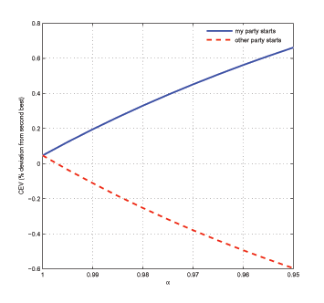
Note: The figure plots, for several degrees of disagreement (measured by α) the difference in welfare (in percentage consumption-equivalent variation (CEV) from second-best), between the case where governments have commitment over their tenure and the case where there is not commitment over the tenure (regardless of π). The continuous line refers to the case where the favorite party starts in office, while the dashed line indicates the case where the adverse party starts. The frequency of turnover is π = .75.
We finally check if there is any circumstance under which an
agent prefers that the adverse party always stays in power. This
may indeed happen when the gain from having political stability
outweighs the cost associated with a provision of a less favorable
public good. For this purpose, we compute the welfare that the
agent would obtain under political turnover (measured by
![]() ) against the welfare he will obtain if
the opposite party will always be in charge. As shown in table
4, welfare can be
higher in the latter case only for a very small level of
disagreement. Indeed, when
) against the welfare he will obtain if
the opposite party will always be in charge. As shown in table
4, welfare can be
higher in the latter case only for a very small level of
disagreement. Indeed, when
![]() having political turnover (as
implied by
having political turnover (as
implied by ![]() ) already gives a welfare level
that is higher by approximately 2.4% of per-period second-best
consumption. This is because in our model, the gains from
commitment are much smaller than the gains from having less
political disagreement.
) already gives a welfare level
that is higher by approximately 2.4% of per-period second-best
consumption. This is because in our model, the gains from
commitment are much smaller than the gains from having less
political disagreement.
Table 4: Welfare implications of political stability (as CEV (%) from second-best)
α |
With Turnover: π = .75 |
With Turnover: π = .5 |
With Adverse Party |
|---|---|---|---|
1.00 |
-0.03 |
-0.04 |
0.00 |
0.99 |
-2.64 |
-2.65 |
-5.09 |
0.98 |
-5.12 |
-5.13 |
-9.70 |
0.97 |
-7.48 |
-7.49 |
-13.88 |
0.96 |
-9.72 |
-9.73 |
-17.69 |
0.95 |
-11.85 |
-11.87 |
-21.17 |
Note: In the first column, we report the welfare implications of having political turnover (π = .75 and π = .5) between parties with different objectives (disagreement measured by α). In the second column we report the welfare that an agent would get if the party providing the less preferred good would always stay in office.
6 Conclusions
Imperfect commitment, political disagreement and political uncertainty may be important sources of inefficient fiscal policies. Our work provides an analysis to distinguish and quantify the effects of each of these forces on the level of debt in a dynamic context.
On the methodological side, our contribution is to develop a framework to analyze the interactions between commitment and political disagreement that can be applied to a wide set of optimal policy problems. In other words, our framework integrates the analysis about the time-inconsistency of optimal policy choices, typical of the dynamic macroeconomic literature, into a political economy model.
On the economic side, we show that imperfect commitment drives the long-run level of debt to zero. Thus, the dependency of debt on initial conditions found in Lucas and Stokey (1983) is shown not to be robust to small departures from the full-commitment assumption. For debt to be driven to zero, it is enough that both the agents and the government anticipate the possibility of the temptation to surprise the economy and to manipulate the interest rate, even if this ultimately never occurs. We find that debt is increased when the government reneges on past promises and is driven to zero when past promises are fulfilled.
Our framework allows the incorporation of political disagreement and imperfect commitment into dynamic macro models. We find that debt is increasing in the level of disagreement among political parties. On the other hand, the frequency of turnover and the degree of commitment do not seem to produce quantitatively important effects. These results are consistent with most of the existing empirical literature. Altogether, our analysis suggests the importance of distinguishing between the degree of polarization among parties and the frequency of political turnover when analyzing the effects of political instability on debt policies.
From a normative point of view, we show that according to our model, the welfare gains from commitment are lower when successive planners disagree about their goals than in the no-disagreement case. With political disagreement, a better commitment technology will not be used to maximize overall welfare but to pursue partisan goals. This result is likely to be present in other institutional settings besides commitment. Whenever a reform allows an institution to achieve a larger set of outcomes, then the welfare gains of such reform are likely to be larger if the institution cares about overall welfare instead of specific interests. We plan to pursue this line of research further both from a theoretical and an empirical point of view.
There are many interesting aspects which deserve further explorations. Among them, we have abstracted from the possibility of default on outstanding debt. This feature is important since it will generate an additional link between the level of debt and the interest rate. This may have an important impact on the interest rate manipulation mechanism, which is crucial in our analysis. Moreover, there will be bigger welfare implications of having different levels of debt.
More generally, our framework would allow us to address several interesting questions. For example, it would be interesting to address some normative implications of this line of research, especially in relationship with fiscal discipline, like limits on deficits and debt holdings, currently imposed on many developed countries by supranational authorities. In this context, considering other forms of political conflicts, voting mechanisms and shocks affecting the economy is an interesting line for future research.
References
Aiyagari, R., Marcet, A., Sargent, T. J., Seppala, J., 2002. Optimal taxation without state-contingent debt. Journal of Political Economy 110, 1220-1254.
Aiyagari, S. R., McGrattan, E. R., 1998. The optimum quantity of debt. Journal of Monetary Economics 42 (3), 447-469.
Alesina, A., Roubini, N., Cohen, G., 1997. Political Cycles and the Macroeconomy. The MIT Press.
Alesina, A., Tabellini, G., 1990. A positive theory of fiscal deficits and government debt. Review of Economic Studies 57 (3), 403-14.
Alt, J. E., Lassen, D. D., 2006. Fiscal transparency, political parties, and debt in oecd countries. European Economic Review 50, 1403-1439.
Azzimonti-Renzo, M., 2004. On the dynamic inefficiency of governments. University of Iowa. Manuscript.
Barro, R. J., 1979. On the determination of the public debt. Journal of Political Economy 87, 940-71.
Barro, R. J., Gordon, D. B., 1983. A positive theory of monetary policy in a natural rate model. Journal of Political Economy 91 (4), 589-610.
Battaglini, M., Coate, S., 2008. A dynamic theory of public spending, taxation and debt. American Economic Review 98 (1), 210-236.
de Haan, J., Sturm, J.-E., 1994. Political and institutional determinants of fiscal policy in the european community. Public Choice 80, 1571-72.
Debortoli, D., Nunes, R., 2006. Loose commitment. Universtat Pompeu Fabra. Manuscript.
Diaz-Gimenez, J., Giovannetti, G., Marimon, R., Teles, P., 2006. Nominal debt as a burden to monetary policy. CREA Barcelona Economics WP. 8.
Ellison, M., Rankin, N., 2007. Optimal monetary policy when lump-sum taxes are unavailable: A reconsideration of the outcomes under commitment and discretion. Journal of Economic Dynamics and Control 31, 219-243.
Franzese, R., 2001. The political economy of public debt: An empirical examination of the oecd postwar experience. Manuscript.
Grilli, V., Masciandaro, D., Tabellini, G., 1991. Political and monetary institutions and public finance policies in the industrial democracies. Economic Policy 13, 3413-92.
Haan, J. D., Sturm, J.-E., 1997. Political and economic determinants of oecd budget deficits and government expenditures: A reinvestigation. European Journal of Political Economy 13, 739-750.
Huber, G., Kocher, M., Sutter, M., 2003. Government strength, power dispersion in governments and budget deficits in oecd-countries: A voting power approach. Public Choice 116, 333-350.
Judd, K. L., 2004. Existence, uniqueness, and computational theory for time consistent equilibria: A hyperbolic discounting example. Stanford University: Manuscript.
Klein, P., Krusell, P., Ríos-Rull, J.-V., 2004. Time consistent public expenditures. CEPR Discussion Papers, 4582, CEPR Discussion Papers.
Krusell, P., Martin, F., Ríos-Rull, J.-V., 2006. Time-consistent debt. Manuscript.
Kumhof, M., Yakadina, I., 2006. Politically optimal fiscal policy. Manuscript.
Kydland, F. E., Prescott, E. C., 1977. Rules rather than discretion: The inconsistency of optimal plans. Journal of Political Economy 85 (3), 473-91.
Lambertini, L., 2004. Are budget deficits used strategically? Manuscript.
Lucas, R. E., Stokey, N. L., 1983. Optimal fiscal and monetary policy in an economy without capital. Journal of Monetary Economics 12 (1), 55-93.
Marcet, A., Marimon, R., 1998. Recursive contracts. Universtat Pompeu Fabra. Working Paper.
Martin, F., 2006. A positive theory of government debt. Manuscript.
Nicolini, J. P., 1998. More on the time consistency of monetary policy. Journal of Monetary Economics 41, 333-350.
Niepelt, D., 2006. Relative asset holdings as a commitment device. Manuscript.
Ortigueira, S., 2006. Markov-perfect taxation. Review of Economic Dynamics 9, 153-178.
Ortigueira, S., Pereira, J., 2008. Markov-perfect optimal fiscal policy: The case of unbalanced budgets. Manuscript.
Persson, T., Svensson, L. E. O., 1989. Why a stubborn conservative would run a deficit: Policy with time-inconsistent preferences. The Quarterly Journal of Economics 104 (2), 325-45.
Persson, T., Tabellini, G., 2000. Political Economics: Explaining Economic Policy. The MIT press.
Roubini, N., Sachs, J. D., 1989. Political and economic determinants of budget deficits in the industrial democracies. European Economic Review 33, 903-938.
Schaumburg, E., Tambalotti, A., 2007. An investigation of the gains from commitment in monetary policy. Journal of Monetary Economics 54 (2), 302-324.
Shin, Y., 2006. Ramsey meets bewley: Optimal government financing with incomplete markets. Manuscript.
Skilling, D., Zeckhauser, R., 2002. Political competition and debt trajectories in Japan and the oecd. Japan and the World Economy 14, 1211-35.
Song, Z., Storesletten, K., Zilibotti, F., 2006. Rotten parents and disciplined children: A politico-economic theory of public expenditure and debt. Manuscript.
Volkerink, B., de Haan, J., 2001. Fragmented government effects on fiscal policy: New evidence, Public Choice 109, 221-242.
Woo, J., 2003. Social polarization, industrialization, and fiscal instability: theory and evidence. Journal of Development Economics 72, 223-252.
Appendix
A The no-commitment case - optimality conditions
The first-order necessary conditions of the planner problem under no-commitment are given by equations (9), (10) and
where it was assumed separability in the utility function, thus
implying
![]() .
.
B The loose commitment case - optimality conditions
The first-order conditions of the planner problem under loose commitment are given by (14) and
In the FOC w.r.t debt, the subscript ![]() denotes next
period variables when previous plans are abandoned.
denotes next
period variables when previous plans are abandoned.
C Alternative formulations of the problem with political disagreement
In this appendix, we explain specific cases that give rise to the disagreement specification considered in the main part of the text.
First Case: Consider that there is a continuum of
households indexed from 0 to 1. The function ![]() represents the weight that each party
represents the weight that each party ![]() assigns to each household
assigns to each household ![]() . The
functions satisfy the following property
. The
functions satisfy the following property
![]() . Each party
believes that a set
. Each party
believes that a set ![]() of households will benefit
from the public expenditure regardless of which party is in power.
However, the remaining households (set
of households will benefit
from the public expenditure regardless of which party is in power.
However, the remaining households (set ![]() ) will not
receive any utility from the public good if the other party is in
power. Denote
) will not
receive any utility from the public good if the other party is in
power. Denote ![]() and
and ![]() by the indicator functions with value 1 if the household is in
group
by the indicator functions with value 1 if the household is in
group ![]() and 0 otherwise. The functions satisfy
the following two properties: i)
and 0 otherwise. The functions satisfy
the following two properties: i)
![]() , and ii)
, and ii)
![]() .
.
Even if a party assigns different weights to individuals, the
private consumption and leisure of all individuals will be the
same. This is because we are assuming separable utility and that
all individuals face the same tax schedule. When party ![]() is in power the public expenditure is denoted by
is in power the public expenditure is denoted by
![]() , while if it is not in power it is
denoted
, while if it is not in power it is
denoted ![]() . Under these conditions, if a given
party is in power it receives the utility:
. Under these conditions, if a given
party is in power it receives the utility:
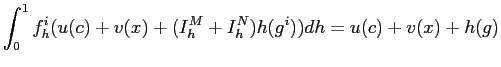
While if the other party is in power, it receives the utility:
where
![]() , and for the
problem to be symmetric we also assume
, and for the
problem to be symmetric we also assume
![]() .
.
If the two parties only want to use the public expenditure with
certain specific groups due to corruption or pork-barrel spending,
then similar arguments to those presented above also lead to an
equivalent specification of disagreement. For instance, consider
the case where each party can make transfers to specific districts.
And in turn the districts supply a local public good that, in
practice, only gives utility to the residents of that district.
This can be for instance the case of a small park, a local road or
a local sports pavilion. For simplicity, assume that
![]() , but party
, but party ![]() only wants to use public expenditure with a subset
only wants to use public expenditure with a subset ![]() of districts, while the other party wants to use the
public expenditure with a subset
of districts, while the other party wants to use the
public expenditure with a subset ![]() . In this
example, the set of districts
. In this
example, the set of districts
![]() will receive transfers
regardless of which party is in power, while the set
will receive transfers
regardless of which party is in power, while the set
![]() will only receive transfers if
party A is in power. The only difference from the previous example
is that
will only receive transfers if
party A is in power. The only difference from the previous example
is that
![]() and
and
![]() .
To obtain an equivalent result, redefine
.
To obtain an equivalent result, redefine
![]() , and
, and
![]() .
.
Second case: Consider that there are two composite public expenditure goods. Each of these public good differs in location, contractors, type and so on. Consider that for both parties each of these goods is a perfect substitute. More formally:
| (A-1) |
where
![]() . Under this specification,
party A will only provide good of type 1 and, viceversa, party B
only provides good of type 2. Consider in addition that the utility
function in
. Under this specification,
party A will only provide good of type 1 and, viceversa, party B
only provides good of type 2. Consider in addition that the utility
function in ![]() is homogenous of degree
is homogenous of degree ![]() , which is satisfied for instance by any power
function. In this case, the utility that each party receives while
in power is simply
, which is satisfied for instance by any power
function. In this case, the utility that each party receives while
in power is simply
![]() , while if the other party
is in power, it receives the utility
, while if the other party
is in power, it receives the utility
![]() . By
denoting
. By
denoting
![]() we obtain the
specification in the main part of the text.
we obtain the
specification in the main part of the text.
In the first case political turnover may occur because the number of households/districts which are better represented by a given party change stochastically. In the second case, political turnover may occur because the mass of agents with a given preference for a type of good change.
D Data and calibration
Table A-1: Debt in the OECD countries in 2006
| Country | Gross | Net |
|---|---|---|
| Australia | 15.0 | -2.8 |
| Austria | 69.1 | 41.8 |
| Belgium | 91.2 | 76.8 |
| Canada | 68.0 | 27.6 |
| Czech Republic | 39.3 | 2.8 |
| Denmark | 39.7 | 6.9 |
| Finland | 48.2 | -60.6 |
| France | 75.3 | 43.0 |
| Germany | 71.3 | 51.9 |
| Greece | 120.6 | 86.9 |
| Hungary | 68.8 | 43.9 |
| Iceland | 24.5 | 8.5 |
| Ireland | 32.5 | 4.9 |
| Italy | 120.8 | 95.4 |
| Japan | 176.2 | 89.5 |
| Korea | 27.9 | -30.2 |
| Luxembourg | 6.6 | - |
| Netherlands | 59.4 | 33.7 |
| New Zealand | 29.8 | -3.5 |
| Norway | 48.1 | -149.3 |
| Poland | 51.7 | 16.6 |
| Portugal | 74.3 | 46.6 |
| Slovak Republic | 38.4 | -11.7 |
| Spain | 46.8 | 26.7 |
| Sweden | 56.0 | -15.0 |
| Switzerland | 54.2 | 21.0 |
| United Kingdom | 47.9 | 41.7 |
| United States | 60.9 | 42.8 |
| Euro Area | 76.8 | 51.3 |
| Total OECD | 76.9 | 44.4 |
General government financial liabilities (percent of nominal GDP). Source: OECD Economic Outlook.
Table A-2: Parameter values
Parameter | Value | Description |
|---|---|---|
β | .96 | discount factor |
φc | .2 | weight of consumption (priv. + publ.) vs. leisure |
φg | .2 | weight of public vs. private consumption |
σx | 3 | Elasticity of leisure |
σc | 2 | Elasticity of private consumption |
σg | .95 | Elasticity of public consumption |
Footnotes
* We are thankful to Klaus Adam, Alberto Bisin, Jordi Galí, Juan Carlos Hatchondo, Albert Marcet and Michael Reiter for many interesting discussions, and to seminar participants at the Society for Economic Dynamics 2007, European Economic Association 2007, Federal Reserve macro conference 2007, Royal Economic Society 2008, Federal Reserve Board, UCLA, Pompeu Fabra, Federal Reserve of New York, Federal Reserve of Boston, UCSD, LSE, ECB, Tolouse, Bank of Italy, Collegio Carlo Alberto, Universita Cattolica, Vigo Macrodynamic Workshop, Simposio de Analisis Economico 2007, University of Oslo, and Norges Bank for their helpful comments. We gratefully acknowledge financial support from CREA and IAE-CSIC (Debortoli) and Fundação para a Ciência e Tecnologia (Nunes). Any remaining errors are our own. The views in this paper are solely the responsibility of the authors and should not be interpreted as reflecting the views of the Board of Governors of the Federal Reserve System or of any other person associated with the Federal Reserve System. Contacts: [email protected], [email protected] Return to text
1. When lump-sum taxes are available, the debt policy is irrelevant, since the so-called Ricardian equivalence holds, see e.g. Barro (1979). Return to text
2. In the appendix, we report the values of the debt/GDP ratio for OECD countries. Return to text
3. For a study about policy choices made by self-interested policymakers see e.g. Alesina et al. (1997) and Persson and Tabellini (2000). Return to text
4. Lucas and Stokey (1983), as we do here, analyzed an economy with complete financial markets. Removing this assumption, as shown by Aiyagari et al. (2002), makes it optimal to accumulate assets. Return to text
5. This happens unless the initial level of debt is sufficiently high. In that case, the improvement in the interest rate is applied to a larger base and can be sufficient to finance the initial tax cut. Return to text
6. As in Lucas and Stokey (1983), we assume that there is still commitment to honor the debt payments. In this paper, the absence of commitment is referred to future policy actions. For a further discussion on this issue see Niepelt (2006). Return to text
7. The dynamic political economy literature has been limited to frameworks where private agents' current choices do not depend on future policy, see e.g. Azimonti-Renzo (2004). Also note that Alesina and Tabellini (1990) by setting the initial level of debt to zero, restrict their analysis to a case where the time inconsistency problem does not play any role. Return to text
8. Ellison and Rankin (2007) and Diaz-Gimenez et al. (2006) also examine the case of indexed debt building on Nicolini (1998). Return to text
9. The absence of uncertainty is for notational convenience. In the presence of exogenous shocks, many of our considerations are still valid under the assumption of complete financial markets. Return to text
10. The opposite happens when b-1 < 0. Return to text
11. The picture is based on the calibration of the next sections. See Lucas and Stokey (1983) for the analytical solution of the model in the case of a quadratic utility function. Return to text
12. If the planner would be allowed to default on his outstanding debt at no cost, then consumers would anticipate it, and there would be no trading. Our assumption can be interpreted as having a default cost being prohibitively high. Return to text
13. See Klein et a. (2004) and Judd (2004) for a detailed discussion on this topic. Ortigueira (2006) analyzes different assumptions on the extent of government's intra-period commitment. Return to text
14. By doing so, we are implicitly assuming differentiability of the function Ψ(bt). We do not have a formal proof about the existence and/or uniqueness of this solution. However, in our numerical exercises we do find a continuous and differentiable solution. Return to text
15. In the present framework, the generalized Euler equation is the derivative of the Lagrangian associated with the problem (8) w.r.t. bt. The other optimality conditions can be found in the appendix. Return to text
16. In this case, the level of government debt should be b = -g*/(1 - β), where g* is the first-best level of public consumption. Return to text
17. Unlike Diaz-Gimenez et al. (2006), our model does not have a cash in advance constraint, and the steady-state level of debt is not only determined by the utility specification on private consumption. Return to text
18. If the initial condition is to the left of the point where Ψb = 0, an increasing path of consumption is instead obtained by accumulating assets over time, until the point where a level of zero taxation is reached and public expenditure can be financed only through the interest payments on the asset holdings. In the subsequent analysis, as it seems more reasonable, we will ignore that case. Return to text
19. If the first-best level of g is relatively low, an increase in production (due to a reduction in debt) will mainly imply a higher consumption instead of a higher g. Return to text
20. We assume separability as it is convenient for our analysis in section 5. Return to text
21. The ratios that we match are c/g, c/y, income taxes (τ), the fraction of time devoted to leisure (x) and the interest rate. We have tried many parameter specifications to check that results do not change qualitatively. Return to text
22. Here we initialize debt at approximately 50% of steady-state GDP under commitment. Even though the steady-state under commitment depends on initial conditions, long-run GDP is almost insensitive to variations of debt. Return to text
23. In this reasoning, we are considering that we are in the upward-sloping part of the Laffer curve. Return to text
24. Schaumburg and Tambalotti (2007) developed a similar methodology than can be applied only to linear-quadratic problems. Our problem is not linear-quadratic and the non-linearity of the policy functions is crucial to determine the level of debt. Return to text
25. For simplicity, we will abstract from other shocks hitting the economy. Return to text
26. In this context, it is equivalent to say that a new government is appointed or that the same government defaults on its past promises. This assumption is relaxed in the next section Return to text
27. Such formulation encompasses all the possible histories of commitment/no-commitment, as shown in Debortoli and Nunes (2006) in a more general framework. Return to text
28. As before, we are only focusing on Markov Perfect equilibria. Return to text
29. Averages are taken with respect to the
realizations of the history of the shock
![]() . Return to text
. Return to text
30. As before, we set as the initial condition for the simulation a level of b0 equal to 50% of GDP. Such initial condition only matters for the values of the full-commitment case. Return to text
31. The steady-state interest rate in the full-commitment and no-commitment cases, is β-1, thus totally independent of debt. In contrast, the level of debt would affect the long-run interest rate, for example, in a model where there is a concern about the default on outstanding debt. However analyzing such case is beyond the scope of this study. Return to text
32. Obviously, there may be other incentives to accumulate debt that are not present in our model. For instance, Ortigueira and Pereira (2008) examine optimal fiscal policy with no commitment in an economy with debt, capital, exogenous labor, and where the tax rate is equal for all sources of income. The authors find that one of the equilibriums is associated with issuance of public debt. In a full commitment model, Kumhof and Yakadina (2006) show that if the planner discounts the future more than what private agents do, then the planner will accumulate debt. Aiyagari and McGrattan (1998) and Shin (2006) find that if heterogeneous agents face undiversifiable idiosyncratic risk that is sufficiently large relative to aggregate risk, the Ramsey planner chooses to issue debt and facilitate the precautionary saving of the private sector. Return to text
33. This symmetry is convenient because the policy functions of both parties are equal. Since in the solution technique we need to employ global methods and the model has two state variables and several decision variables, relaxing this symmetry significantly complicates our analysis. In a simpler framework, Azimonti-Renzo (2004) considers asymmetric cases. Return to text
34. The average length of a government is given by 1/(1-π). A benchmark of 4 years corresponds to π = 0.75. While π = 0.25 or π = 0 correspond to very short average tenures of 1.3 years and 1 year respectively. When π changes between 0.9 and 0.25 debt is not substantially affected. Return to text
35. The authors do not present a regression with the average tenure and the evidence regarding this variable is only suggestive. The finding that coalition governments tend to accumulate more deficits has been challenged for instance by Haan and Sturm (1997). See also Alesina et al. (1997) for some evidence supporting Roubini and Sachs. Return to text
36. Since the problem is fully symmetric, the difference in the utilities of the two types of agents is only due to the type of party starting in office. Return to text
37. A value of π = .75 implies that a government is replaced on average every four periods (i.e. four years under our calibration). This is why we take it is as benchmark. Return to text
This version is optimized for use by screen readers. Descriptions for all mathematical expressions are provided in LaTex format. A printable pdf version is available. Return to text