Skip to: [Printable Version (PDF)]

Board of Governors of the Federal Reserve System
International Finance Discussion Papers
Number 949, September 2008 --- Screen Reader Version*

Expected Consumption Growth from Cross-Country Surveys: Implications for Assessing International Capital Markets

Charles Engel, University of Wisconsin and NBER^*
John H. Rogers, Board of Governors of the Federal Reserve

NOTE: International Finance Discussion Papers are preliminary materials circulated to stimulate discussion and critical comment. References in publications to International Finance Discussion Papers (other than an acknowledgment that the writer has had access to unpublished material) should be cleared with the author or authors. Recent IFDPs are available on the Web at http://www.federalreserve.gov/pubs/ifdp/. This paper can be downloaded without charge from the Social Science Research Network electronic library at http://www.ssrn.com/.

Abstract:

Survey data show that the expected growth rates of consumption across countries vary widely and are not highly correlated. This data contradicts the simplest of open-economy models in which there is a freely traded non- state-contingent bond and purchasing power parity holds. We explore two alternative explanations for the finding: that households in each country in effect face different ex ante real interest rates or that there are significant credit constraints, so that expected consumption growth rates are driven largely by expected income growth. The empirical evidence strongly supports the latter hypothesis. These findings challenge the modeling of consumption that is at the heart of many, if not most, macroeconomic models.

Keywords: Consumption Euler equation, survey data, international capital mobility

JEL classification: E21, F32, F41

1  Introduction

The present-value model of the current account is an intuitively appealing approach to understanding international imbalances. The starting point of the model is the observation that a current account imbalance implies a change in a country's net external asset position. A country running a surplus, for example, must be acquiring claims on the rest of the world. The model focuses on the intertemporal decision of households and firms. Specifically, a country will borrow when desired investment by firms exceeds desired saving by households. An essential building block of the model is the Euler equation for the household, which determines, in essence, expected consumption growth as a function of real interest rates.

While the present-value model is intuitively appealing, its empirical performance is spotty. Nason and Rogers (2006) put it more bluntly: "Tests of the present-value model (PVM) of the current account are frequently flatly rejected by the data." Examples of such rejections can be found in Sheffrin and Woo (1990a, b), Otto (1992), and Ghosh (1995). Some modifications of the basic PVM in these early papers have been found to improve the fit of the model. Bergin and Sheffrin (2000) allow for time-varying real interest rates and real exchange rates, and find the fit of the model is improved. Similarly, Nason and Rogers (2006) find that allowing for a time-varying world real interest rate enhances the empirical performance of the model. Gruber (2004) modifies the standard representation of preferences to allow for habit persistence. This modification allows the PVM to produce a current account whose volatility is more in line with empirical observations. Kano (forthcoming) argues that the crucial factor in the failure of the present-value model of the current account in early tests is that they failed to capture the consumption-tilting. According to Kano (2007), standard tests of the PVM are not able to distinguish between time-varying world real interest rates and habit persistence in preferences.¹

A potential problem for the PVM is the Euler equation for household consumption. From a number of different sources, there appears to be little support for the Euler equation as a description of consumption behavior, at least using standard models of preferences. In the PVM, the ability of households to borrow and lend freely on international capital markets allows for smoothing of intertemporal income risk. The present-value model derives the conclusion that consumption at any point in time should equal the annuity value of wealth, including lifetime discounted labor income. With a constant intertemporal rate of substitution (CIES), expected consumption growth approximately equals the real interest rate.

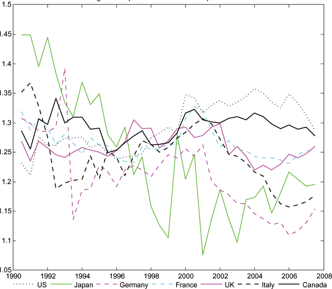
In the simplest versions of the PVM, if capital markets are well integrated, all households in the world face a common world interest rate. It follows that under the CIES assumption, expected consumption growth should be equalized across countries. Our paper uses a unique data set to provide some direct evidence on this building block of the PVM. Specifically, we make use of surveys of expected consumption growth conducted by Consensus Forecasts. We make use of surveys of economic forecasters in the G7 countries that twice a year (April and October) record the median forecasts of long-run consumption growth.

It is evident (see Figure 1) that expected consumption growth is not equalized across countries. Each survey records expected consumption growth for the current year, each of the next five years, and then the expected average consumption growth rate for years 6-10 from the current year. From these surveys, we can construct expected 10-year consumption growth rates as the compounded annual expected growth rates.² Figure 1 plots the 10-year expected growth rates from each survey. Clearly the forecasters do not expect consumption to grow at equal rates across countries. According to the figure, cross-country expected consumption growth differentials can be as large as 20-25 percentage points, two or more percentage points per year on average. In addition, there appears to be very little co-movement in the expected consumption growth rates, contrary to a basic prediction of the PVM of the current account.

One possible explanation of Figure 1 is that households in each of the G7 countries face different ex ante real interest rates. There are two possible general reasons why households in different countries might not be able to borrow and lend at the same real interest rate. The real interest differential between two countries can be written as the deviation from uncovered interest parity (which pertains to nominal interest rates and exchange rates) and the expected change in the real interest rate. Deviations from uncovered interest parity might arise because markets for interest-bearing securities are not perfectly integrated, or because there are risk considerations. On the other hand, even if capital markets are well integrated and risk premiums are low, there may be large real interest differentials if purchasing power parity does not hold. If there are expected changes in the real exchange rates between a pair of countries, then the effective consumption real interest rates will be different in the two countries.³

While we cannot distinguish the cause for real interest differentials, our survey data provides a direct measure of the differential. That is because we can use a measure of the long-term (10-year) nominal interest rate in combination with the survey's measure of expected inflation over the upcoming 10 years. The same Consensus Forecast survey that collects forecasts of consumption growth also gathers inflation forecasts for a horizon that parallels the consumption forecasts. A possible explanation for Figure 1 - the dispersion across countries of consumption growth forecasts - is that indeed household Euler equations hold, but that households in different countries face different real interest rates. Our data allow us to gauge how much of the differences in forecasts of consumption growth can be attributed to real interest differentials.

But perhaps consumption Euler equations (in conjunction with CIES preferences) are not a useful description of consumption behavior. Figure 2 hints at an alternative class of models for aggregate consumption. The Consensus Forecasts constructs measures of expected GDP growth, which again parallel the forecasts of consumption growth and inflation in terms of the horizon and coverage of the surveys. In Figure 2, we have plotted the expected 10-year GDP growth rates and consumption growth rates for each of the G7 countries. It is clear that these forecasts move closely together. ⁴

But Figure 2 shows that expected consumption growth may be too closely related to expected income growth. There are a couple of possible explanations for such a tight link. It may be that many households are credit constrained. Borrowing and lending is not so easy, and consumption is more closely tied to current income than the PVM allows. Or, it may be that capital markets are available to households, but consumption behavior is not as forward looking as the PVM assumes. In either case, we might find that expected consumption growth is more closely tied to expected income growth than to ex ante real interest rates. In Figure 3 we plot expected consumption growth against a measure of an expected 10-year real interest rate for each country. The latter is constructed from the Consensus forecasts of nominal interest rates and inflation rates. The correlation does not appear to be nearly as tight as that between expected consumption growth and expected real income growth.

The remainder of this paper tests more formally the propositions outlined above. We investigate how much of differences in expected consumption growth rates across countries can be explained by real interest differentials versus differences in expected income growth. As Figures 2 and 3 suggest, we will find a much stronger role for expected income growth. This undermines one of the key building blocks of the PVM.

The theory is well known, so section 2 provides only a brief review. In section 3, we describe the data in greater detail and discuss our empirical specification. Section 4 presents results, and section 5 discusses the implications of the findings.

2  Model Background

Here we review the implications of the PVM for cross-country expected consumption. Assume households have a period utility given by $\frac{1} {1-\rho}C_{t}^{1-\rho}$. $C_{t}$ is the consumption aggregate for the household. They maximize the expected present discounted value of utility, with a constant discount factor given by $\beta$. As is well known, the Euler equation representing intertemporal substitution between consumption at time t and consumption in 10 years, $C_{t+10}$, is given by:

$$C_{t}^{-\rho} =\beta E_{t} \left( {R_{t}^{10} C_{t+10}^{-\rho} } \right) .$$

Here, $R_{t}^{10}$ is the real rate of return on an interest-bearing bond with a maturity of 10 years.

Hereinafter, we will assume that we can approximate this Euler equation by:

$$C_{t}^{-\rho} =\beta R_{t,10} C_{t,t+10}^{-\rho} .$$

$C_{t,t+10}$ refers to the expectation at time t of period t+10 consumption as taken from our survey data. $R_{t,10}$ is the expected real return on a nominal bond with a ten-year maturity. As discussed above, we construct this measure by deflating the nominal yield on a 10-year bond by the survey measure of expected inflation. Section 3 provides details on the data construction. An appendix elaborates on the implications of this approximation of the Euler equation.

With this approximation, we get:

$$C_{t,t+10} /C_{t} =\beta^{1/\rho}(R_{t,10} )^{1/\rho}$$ (1)

If households in every country face the same real interest rate, and have the same preferences, they have the same expected consumption growth rate.

As noted in section 1, the survey data are not consistent with this prediction. We consider two general types of explanations for the observed differences in expected consumption growth: the real interest rate is different across countries, because capital markets are not perfect or PPP does not hold so the real return is different; or, consumption is tied to income. Under the former assumption, all households maximize utility, and equation (1) holds for everyone in each country.

Under the alternative assumption, consumption growth is tied to income growth. We model this in an ad hoc way. Perhaps consumers follow a simple rule of thumb, or perhaps there are capital market imperfections that tie consumption to current income. We let $C_{t}^{R}$ denote consumption of this group, and posit an equation of the form:

$$C_{t,t+10}^{R} /C_{t}^{R} =a+c\left( {Y_{t,t+10}^{R} /Y_{t}^{R} } \right)$$ (2)

We can nest the two theories in a general model, where a fraction $\mu$ follow equation (1) and $1-\mu$ follow rules of thumb. Then, the aggregate expected growth rate of consumption is approximately a weighted average of the right-hand-side of the two equations. Specifically, let $C_{t}^{U}$ be consumption of utility-maximizing consumers. Rewrite equation (1) as:

$$C_{t,t+10}^{U} =\beta^{1/\rho}(R_{t,10} )^{1/\rho}C_{t}^{U} =\beta^{1/\rho}(R_{t,10} )^{1/\rho}\mu C_{t}$$ (3)

Rewrite equation (2) as

$$C_{t,t+10}^{R} =\left[ {a+c\left( {Y_{t,t+10}^{R} /Y_{t}^{R} } \right) } \right] C_{t}^{R} =\left[ {a+c\left( {Y_{t,t+10}^{R} /Y_{t}^{R} } \right) } \right] (1-\mu)C_{t}$$ (4)

Adding (3) and (4) together, and dividing by $C_{t}$, we get:

$$C_{t,t+10} /C_{t} =(1-\mu)a+\mu\beta^{1/\rho}(R_{t,10} )^{1/\rho} +(1-\mu)c\left( {Y_{t,t+10}^{R} /Y_{t}^{R} } \right)$$ (5)

Equation (5) suggests the empirical specification we pursue. In each country, we ask whether we can explain expected consumption growth using expected real interest rates and expected output growth.

3  Data and Empirical Specification

Our data come from surveys conducted by Consensus Forecasts. Beginning in 1989, Consensus Forecasts has sent a form each month to professional forecasters inquiring about their outlook for several macroeconomic and financial market variables for the next two years. Each April and October, the survey participants are also asked about their forecasts at longer horizons, up to ten years out; we use these long-horizons forecasts in this paper. Forms are sent the first Tuesday or Wednesday of the month, with a request that responses be received by the following Monday. The response deadline of the second Monday of the month is chosen because most announcements of monthly macroeconomic data occur in the first week of the month. Survey results are published on the Thursday after the Monday deadline. Consensus reports the mean forecast across survey respondents, which number in the range of two or three dozen depending on the country.$^{ }$⁵ The Consensus Forecasts survey data has been used in many academic papers, including Engel, Mark, and West (2008), Engel and Rogers (2006), Ghysels and Wright (forthcoming).

We construct our measures of expected consumption growth, real interest rates, and expected out put growth as follows:

10-year expected consumption growth:

The April and the October surveys are treated differently depending on how the forecasts of current year variables are handled.

April: Take April 2006 as an example. The survey reports expected consumption growth rates for each year between 2006 and 2011, and then an average for 2012-2016. Let $E_{t} G_{t,t+1}^{C}$ be the gross growth rate forecast for 2006. Similarly, $E_{t} G_{t+1,t+2}^{C}$,..., $E_{t} G_{t+5,t+6}^{C}$, refer to the growth rates expected in 2006 for 2007-2011. Then use the notation $E_{t} G_{\infty}^{C}$ to denote the expected growth rate for the 2012-2016 period. The 10-year expected growth rate for April 2006, $G_{t,10}^{C}$ is:

$$G_{t,10}^{C} =\left( {E_{t} G_{t,t+1}^{C} } \right) \left( {E_{t} G_{t+1,t+2}^{C} } \right) \left( {E_{t} G_{t+2,t+3}^{C} } \right) \left( {E_{t} G_{t+3,t+4}^{C} } \right) \left( {E_{t} G_{t+4,t+5}^{C} } \right) \left( {E_{t} G_{t+5,t+6}^{C} } \right) \left( {E_{t} G_{t,\infty}^{C} } \right) ^{4}.$$

October: Now take October 2006 as an example. Here, $E_{t} G_{t,t+1}^{C}$ is the expected growth rate of consumption for 2007. In April of each year, the first expected growth rate is the expected growth rate for the current year, but for the October survey, the first expected growth rate is the expected growth rate for the next year. $E_{t} G_{t+1,t+2}^{C}$,..., $E_{t} G_{t+4,t+5}^{C}$ refer to the expected growth rates for 2008-2011. $E_{t} G_{\infty}^{C}$ represents the expected consumption growth rate for the final 2012-2016 period. Then we calculate the 10-year expected growth rate for October 2006, $G_{t,10}^{C}$, as

$$G_{t,10}^{C} =\left( {E_{t} G_{t,t+1}^{C} } \right) \left( {E_{t} G_{t+1,t+2}^{C} } \right) \left( {E_{t} G_{t+2,t+3}^{C} } \right) \left( {E_{t} G_{t+3,t+4}^{C} } \right) \left( {E_{t} G_{t+4,t+5}^{C} } \right) \left( {E_{t} G_{t,\infty}^{C} } \right) ^{5}.$$

10-year expected output growth - Calculated the same way as expected consumption growth. Call this $G_{t,10}^{Y}$

10-year expected inflation - Calculated the same way as expected consumption growth.

10-year nominal interest rate - In both April and October of each year, Consensus Forecasts reports the actual 10-year bond yield on the date of the survey.

10-year real interest rate - We take the 10-year gross nominal interest rate described above, and divide by the 10-year gross expected inflation described above. Call this $R_{t,10}$

Equation (5) inspires the following empirical specification, which we estimate for each of the G7 countries individually⁶:

$$C_{t,t+10} /C_{t} =b_{0} +b_{1} (R_{t,10} )^{1/\rho}+b_{2} (Y_{t,t+10} /Y_{t} ).$$ (6)

We do not estimate this regression over the entire sample, but instead perform rolling regressions using 10 years of data (and therefore 20 observations.) Our reasoning is that if indeed the consumption growth rates of the expected utility maximizing households and the rule-of-thumb households are different, then their weight $\mu$ in aggregate consumption might evolve over time. Alternatively, the rolling regressions can be viewed as a simple way of determining whether the importance of the two explanatory variables has changed over time, or as a way of accounting for structural breaks in the series that are due, say, to revisions to data collection procedures.

We estimate equation (6) using OLS regressions imposing $\rho=2$ (a typical value used in macroeconomic calibrations). In addition to the country-by-country estimates, we undertake panel estimation of equation (6). Here and in all panel estimates we impose $\rho=2$ for all countries, impose that $b_{1}$ and $b_{2}$ are common across all countries, but allow the intercepts, $b_{0}$, to be country-specific; panel OLS standard errors are calculated.

Ultimately, we want to explain why $C_{t,t+10} /C_{t}$ is different than $C_{t,t+10}^{W} /C_{t}^{W}$ where the $W$ superscript refers to world expected consumption growth. That suggests the following specification, where we divide variables by $C_{t,t+10}^{W} /C_{t}^{W}$:

$$[(C_{t,t+10} /C_{t} )/(C_{t,t+10}^{W} /C_{t}^{W} )]=d_{0} +d_{1} [(R_{t,10} )^{1/\rho}/(C_{t,t+10}^{W} /C_{t}^{W} )]+d_{2} [(Y_{t,t+10} /Y_{t} )./(C_{t,t+10}^{W} /C_{t}^{W} )]$$ (7)

$C_{t,t+10}^{W} /C_{t}^{W}$ is a measure of the expected growth rate of G7 consumption, where G7 consumption growth is measured as a weighted average of consumption growth in each country.$^{ }$⁷

Under the standard model, $C_{t,t+10}^{W} /C_{t}^{W}$ should be proportional to $(R_{t,10}^{W} )^{1/\rho}$, the world real interest rate (to the $1/\rho$ power) if each country faces the same real interest rate. Equation (7) then explains the deviation of expected consumption growth in each country from expected G7 consumption growth as a function of the deviation of each country's real interest rate from the world real interest rate implied by the model (again, taken to the $1/\rho$ power), and to expected GDP growth in each country relative to expected consumption growth in the G7.

As with equation (6), we estimate (7) country-by-country and as a panel, imposing $\rho=2$ so that the model is linear.

In addition to (6) and (7), we consider logarithmic specifications:

$$c_{t,t+10} -c_{t} =e_{0} +e_{1} \ln(R_{t,10} )+e_{2} (y_{t,t+10} -y_{t} )$$ (8)

and

$$[(c_{t,t+10} -c_{t} )-(c_{t,t+10}^{W} -c_{t}^{W} )]=f_{0} +f_{1} \ln[(R_{t,10} )^{1/\rho}/(C_{t,t+10}^{W} /C_{t}^{W} )]+d_{2} [(y_{t,t+10} -y_{t} )-(c_{t,t+10}^{W} -c_{t}^{W} )]$$ (9)

where the lower case c and y refer to logs of consumption and output. Finally, specification (9) suggests a more general equation in which the effect of world consumption growth on domestic consumption growth is not restricted:

$$c_{t,t+10} -c_{t} =g_{0} +g_{1} \ln(R_{t,10} )+g_{2} (y_{t,t+10} -y_{t} )+g_{3} (c_{t,t+10}^{W} -c_{t}^{W} )$$ (10)

As with equations (6) and (7), we perform both country-by-country and panel estimation of each of these equations.

4  Empirical Results

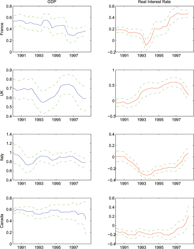
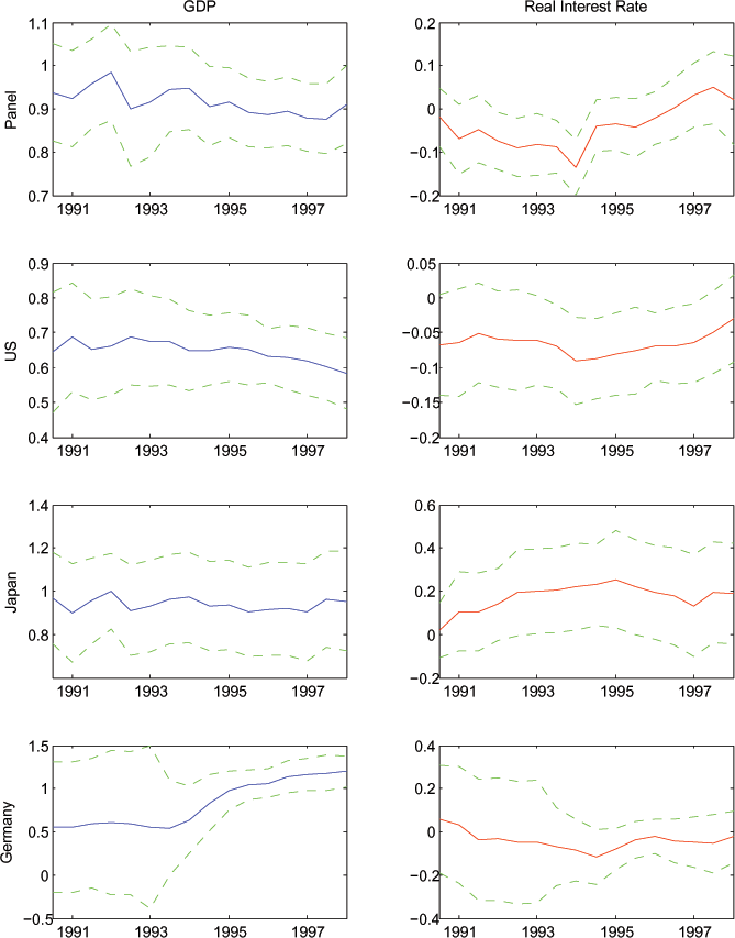
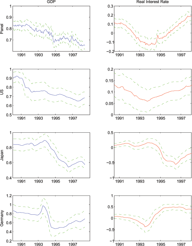
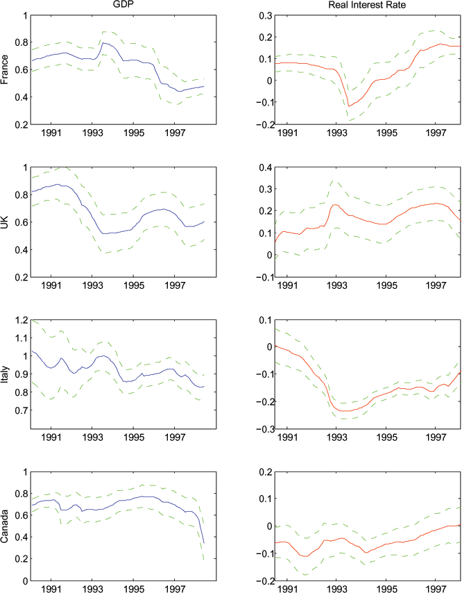
The results for all of our specifications are displayed graphically in Figures 4-8. Each Figure corresponds to results from one equation. (Figure 4 reports results of estimation of equation (6), Figure 5 of equation (7), etc.) In each Figure, we report first the panel estimates of the slope coefficients, followed by estimates of the slope coefficients for each country. We report the results graphically because we estimate rolling regressions, so we can conveniently report coefficient estimates and confidence intervals visually.

In Figure 4, the column on the left hand side of the figures displays the rolling-sample estimates of $b_{1}$, the coefficient on GDP from equation (6). The right-hand-side columns display the estimates of $b_{2}$, the coefficient on the real interest rate. Plus and minus two (OLS) standard error bands are also displayed. The first row of the figures displays the estimates of $b_{1}$ and $b_{2}$ for the panel of countries; each of the remaining rows presents estimates for one of the G7 countries, beginning with the U.S. in row two. The sample begins in 1990; hence the first estimate displayed is for the 10-year period 1990-99. The final estimate is for 1998-2007.

The results are striking. The coefficients on GDP growth are always positive and statistically significant. For many countries the estimate is near unity. In fact, except for the U.S., the confidence interval contains unity for the estimates over most of the windows, and for all of the estimates for some countries. The panel estimated coefficient on expected income growth is slightly below one, and the confidence interval never includes one, reflecting the role of the U.S. in pulling down the coefficient estimate. But even in the U.S., the coefficient on expected income growth is quite high, in the range of 0.60.

On the other hand, for the real interest rate, the point estimates are more often negative than of the expected positive sign, and are rarely statistically different from zero in the country-by-country analysis. For the panel, there is a small window where the coefficient is significantly different than zero, but it is significantly negative. These findings offer very little comfort to the theory that expected consumption growth in each country is determined by the local ex ante real interest rate.

Figure 5 displays the estimates from equation (7), the specification where we transform the variables in the baseline specification to be ratios of world consumption growth. The transformation has no material effect on the estimated coefficients. The only noticeable change is that the coefficient on expected income growth in the U.S. regression is lower than in the unscaled version of the model. However, this mechanically follows because the U.S. share of total "world" consumption is large.

In Figures 6 and 7 we display estimates of equations (8) and (9), respectively, the log specifications of equations (6) and (7). Once again the results are quite robust: expected consumption growth tracks expected GDP growth very tightly for each of the G7 countries. In many cases, the two series move nearly one for one. On the other hand, expected consumption growth is essentially uncorrelated with expected real interest rate in the G7.

As we have noted, the primary exception to the general pattern of results is the U.S., where consumption and GDP growth move considerably less than one for one. Engel and Rogers (2006) present favorable results for a simple present-value model of the current account in U.S. data, a finding that is not replicated (in unpublished work) for other G7 countries. It may appear, then, that U.S. consumers are more forward looking than consumers in the other countries. However, figures 4-8 of the current paper show that the correlation between U.S. consumption growth and real interest rate is zero or negative.

Finally, in Figure 8 we display results when we add world consumption growth to the right hand side of the log specification whose results were displayed in Figure 6. In the country-by-country analysis, the general pattern of results continues to hold: the coefficients on expected income are significantly different from zero and usually near unity (except for the U.S.), and the coefficients on real interest rates are generally not significantly different than zero. Usually the coefficient on world consumption growth is near zero. We note, however, that for some windows for a few countries, the coefficient is significantly positive, and in those windows the estimated coefficient on expected income is correspondingly lower. Finally, we note that in the panel estimates, the coefficient on world consumption and the world interest rate are generally insignificantly different than zero, while the estimated coefficient on expected income growth remains significantly positive and close to unity.

4.1  Robustness: results using one-year expectations

The Appendix contains the results of a check for robustness to constructing our expectations variables at one-year horizons rather than ten-year. Figure A-1 is analogous to Figure 1, and hence depicts the expected consumption growth rates by country. One-year ahead expected consumption growth rates also differ significantly across countries. Differentials are typically larger at the one-year horizon than at the ten-year horizon. This is as one would expect, as the ten-year ahead expectations are presumably less influenced by business cycle considerations.

In Figure A-2, we plot the expected one-year GDP growth rates and consumption growth rates for each of the G7 countries. As we saw in Figure 2 for the ten-year growth rates, these short-horizon forecasts of GDP and consumption growth rate move closely together. In Figure A-3 we plot expected consumption growth against expected one-year real interest rate for each country. The correlation once again does not appear to be nearly as tight as that between expected consumption growth and expected real income growth.

Finally, Figure A-4 presents the regression results for the specification in logs, equation (8). Figure 6 presents the analogous results for the long-horizon expectations. We see that expected consumption growth has little to do with the real interest rate. It is connected closely to expected GDP growth, as observed in earlier results, though the coefficient with the one-year expectations is lower than unity and in many cases appears to be falling over time.

Comparing our results with our findings using 10-year expectations, we see that expected consumption growth over the 1-year horizon is less responsive to expected income growth over the same horizon than was true for the 10-year expectations. That is, the coefficient on expected income growth in equation (8) is significantly less than one for all countries in the 1-year horizon regressions, while it is close to one for nearly all countries in the 10-year horizon regressions.

On the other hand, in neither the 1-year nor 10-year data is there much of a link between expected consumption growth and real interest rates. Frequently the coefficients are insignificantly different than zero, or negative. Apparently, intertemporal consumption decisions are not very much influenced by changes in real interest rates, at least to the extent that these survey measures of expectations reflect household expectations.

This pattern of empirical results is puzzling from the standpoint of standard models of consumption. The model based on expected utility maximization relates the level of consumption to the expected present discounted value of income flows, and the expected growth in consumption to the real interest rate. Here, in essence, we find that there is a sort of consumption smoothing going on - the 1-year expected growth rate of consumption and the 1-year expected growth rate of income are less closely tied than the 10-year rates. But it is the expected growth-rate of consumption in the long run, not the level, that is connected to the long-run expected growth of income. And the expected real interest rate seems to have little influence on consumption decisions at any horizon.

5  Conclusions

Our survey data show that the expected growth rates of consumption across countries vary widely and are not highly correlated (Figure 1). This data contradicts the simplest of open-economy models in which there is a freely traded non-state-contingent bond and purchasing power parity holds. We have explored two alternative explanations for the finding: The first posits that the inequality in expected consumption growth rates arises because households in each country in effect face different ex ante real interest rates. The second hypothesis is that there are significant credit constraints, so that expected consumption growth rates are not determined by ex ante real interest rates, but instead are driven largely by expected income growth. The empirical evidence strongly supports the latter hypothesis.

These findings are not just a challenge for open-economy macroeconomists, because they challenge the modeling of consumption that is at the heart of many, if not most, macroeconomic models. We find that expected consumption growth is not determined by ex ante real interest rates. That relation is central in many macro models.

One point worth emphasizing is that these findings also pertain to the recent literature on the consumption-real exchange rate anomaly, or Backus-Smith puzzle.⁸ When agents can trade a complete set of contingent claims denominated in a single numeraire (such as a currency), but purchasing power parity does not hold, then if agents have power utility functions, the relative growth rates of consumption in two countries should equal the real exchange rate growth. This theory is a special case of the one we have examined. If markets are complete, actual ex post relative consumption growth should equal ex post real exchange rate growth. But in that setting, the relationship must obviously hold ex ante as well if expectations are rational: expected relative consumption growth should equal the expected real exchange rate change, which in turn will equal the ex ante real interest differential. This is the equation that we test.

There are many caveats to our study. The first is that our survey may not measure the market's true expectations of consumption growth. The forecasters in our survey may not do as good a job forecasting consumption growth as households do, or there may be some bias in their reporting of expected consumption growth.$^{ }$⁹

While we recognize that our survey measures expected consumption growth with error, the usual method of testing whether expected consumption growth is equal to the ex ante real interest rate is also subject to errors. The standard methodology is to assume expectations are rational, and then to use ex post consumption growth to measure ex ante consumption growth, with an error that is uncorrelated with the information used to formulate expectations. If expectations are rational, that approach should work if the data sample is sufficiently large. However, if consumption growth is persistent and/or the data generating process for consumption growth is subject to periodic regime changes, then ex post measurement may not yield a very useful measurement of ex ante expectations given available sample sizes.

Of course, the other criticism of the standard methodology is that it requires incorporating rational expectations as part of the null hypothesis. Survey-based measures of expectations place no such restriction. Moreover, there is a middle ground where survey measures still may be advantageous. If income is subject to regime changes, households may not be immediately aware of the new data generating process. There may be a period of learning. Even when learning is optimal, the problems with using a small data sample of ex post consumption to measure ex ante expectations are compounded.

Another shortcoming of our approach arises from the fact that the Euler equation does not exactly relate expected consumption growth to real interest rates, even when households have a power utility function. Instead, it equates the expectation of a function of consumption growth to the real interest rate. We are using a first-order approximation to the Euler equation, but there may be some information lost that a higher-order approximation would capture. It seems unlikely, however, that inclusion of these higher moments could account for the high correlation of expected consumption growth with expected income growth.

Our approach does not allow for heterogeneity among agents. Perhaps households have different information sets, and therefore have different expectations of consumption. Indeed, our measure of expected consumption averages forecasts over the reported forecasts from several dozen professionals. Smith and Yetman (2007) have examined the properties of forecasts of consumption and real interest rates (at horizons up to one year), using data drawn from individual forecasters. They use a panel approach to estimating the parameters of the Euler equation based on individual forecasts, and do not attempt to relate consumption forecasts to income forecasts. However, their findings are not encouraging for Euler equations, as they find overall a negative relationship between expected consumption growth and ex ante real interest rates.

There may be heterogeneity of another sort, arising from the fact that individual lifetimes are finite. Models with overlapping generations of agents with imperfect bequest motives have been used in recent literature to explore the behavior of current accounts.¹⁰ Further exploration may determine if such models could account for either our empirical findings or those of Smith and Yetman (2007).

A possible explanation for our finding that expected consumption growth is not closely related to ex ante real interest rates is that we have done a poor job modeling preferences. While the class of models that relate ex ante consumption growth to ex ante real interest rates, to a first-order approximation, extends beyond the simple power utility function, this still represents a potentially narrow assumption about utility. We reiterate, however, that this relationship is an essential element of many macroeconomic models. But allowing for a general specification of preferences may break down the relationship between expected consumption growth and the real interest rate. One possible elaboration of preferences is simply to allow non-separability between leisure and consumption. Head, Mattina, and Smith (2004) consider this as a possible explanation for the Backus-Smith puzzle, but in fact find that this non-separability is of little help. Recently, Jaimovich and Rebelo (2007) have proposed a specification in which consumption and leisure are non-separable, to help explain the macroeconomic reaction to news in an open economy.

Cochrane (2005) has, in essence, advocated an approach in which minimal assumptions are imposed on preferences. Under his approach, we might do one of two things. We could assume the Euler equation is true, and use the Euler equation to back out implications about preferences. Campbell and Cochrane (1999) is an example of this approach. Alternatively, we could examine aspects of Euler equations that are not dependent on preferences, such as examining the consistency of Euler equations for pricing different assets. Brandt, Cochrane, and Santa-Clara (2006) is an application of this approach to international asset prices.

The challenge, however, is to reconcile this approach with our finding that expected consumption growth is so closely related to expected income growth. Are there plausible preference specifications that can deliver this result?

Now we come full circle. If indeed there are significant impediments to international capital flows, aggregate consumption growth might look like it would in a closed economy. Specifically, in a closed economy, consumption growth must equal income growth (or, at least, income net of investment and government spending.) One possible reaction to our findings then is the following: Expected consumption growth matches expected income growth because opportunities for international asset trade are limited. Expected consumption growth is not closely determined by the ex ante real interest rate because there is a time-varying pricing kernel that we do not capture well in our model with power utility. (That is, à la Cochrane, the Euler equation does not put a directly measurable restriction on expected consumption growth.)

In the end, it is an open question whether this explanation for our findings is more plausible than the alternative that credit constraints are important so that aggregate consumption behavior is not well described by Euler equations. Or perhaps there are elements of truth to both stories. In either case, the empirical findings present a challenge to the building block of many macroeconomic models, in which expected consumption growth is driven by the ex ante real interest rate.

References

Ang, A., G. Bekaert, and M. Wei, 2007, "Do Macro Variables, Asset Markets, or Surveys Forecast Inflation Better?" Journal of Monetary Economics, Vol. 54, No. 4, pp. 1163-1212.

Backus, D.K., and G.W. Smith, 1993, "Consumption and Real Exchange Rates in Dynamic Economies with Nontraded Goods," Journal of International Economics, Vol. 35, Nos. 3-4, pp. 297-316.

Bergin, P. R., and S.M. Sheffrin, 2000, "Interest Rates, Exchange Rates and Present Value Models of the Current Account," The Economic Journal, Vol. 110, No. 463, pp. 535-58.

Brandt, M.W., J.H. Cochrane, and P. Santa-Clara, 2006, "International Risk Sharing is Better than You Think, or Exchange Rates are Too Smooth," Journal of Monetary Economics, Vol. 53, No. 4, pp. 671-98.

Caballero, R.J., E. Farhi, and P.O. Gourinchas, 2008, "An Equilibrium Model of 'Global Imbalances' and Low Interest Rates," American Economic Review, Vol. 98, No. 1, pp. 358-93.

Campbell, J.Y., and J.H. Cochrane, 1987, "Permanent Income, Current Income, and Consumption," NBER working paper #2436.

Campbell, J.Y., and N.G. Mankiw, 1999, "By Force of Habit: A Consumption-Based Explanation of Aggregate Stock-Market Behavior," Journal of Political Economy, Vol. 107, No. 2, pp. 205-50.

Cochrane, J.H., 2005, Asset Pricing (Princeton: Princeton University Press).

Corsetti, G., L. Dedola, and S. Leduc, 2008, "International Risk-Sharing and the Transmission of Productivity Shocks," Review of Economic Studies, Vol. 75, No. 2, pp. 443-73.

Croushore, D., 2007, "An Evaluation of Inflation Forecasts from Surveys Using Real Time Data." Working Paper, University of Richmond Robins School of Business.

Engel, C., N.C. Mark, and K.D. West, 2008, "Exchange Rate Models are Not as Bad as You Think," NBER Macroeconomics Annual 2007, Vol. 22, pp. 381-440.

Engel, C., and J.H. Rogers, 2006, "The U.S. Current Account Deficit and the Expected Share of World Output," Journal of Monetary Economics, Vol. 53, No. 5, pp. 1063-93.

Ferrero, A., 2007, "The Long-Run Determinants of the U.S. External Imbalances." Federal Reserve Bank of New York Staff Report no. 295.

Ghosh, A.R., 1995, "International Capital Mobility amongst the Major Industrialised Countries: Too Little or Too Much?" The Economic Journal, Vol. 105, No. 428, pp. 107-28.

Ghysels, E., and J.H. Wright, "Forecasting Professional Forecasters," Journal of Business and Economics Statistics, forthcoming.

Gruber, J.W., 2004, "A Present Value Test of Habits and the Current Account," Journal of Monetary Economics, Vol. 51, No. 7, pp. 1495-1507.

Head, A.C., T.D. Mattina, and G.W. Smith, 2004, "Real Exchange Rates, Preferences, and Incomplete Markets: Evidence, 1961-2001," Canadian Journal of Economics, Vol. 37, No. 3, pp. 782-801.

Jaimovich, N., and S. Rebelo, 2007, "News and Business Cycles in Open Economies." National Bureau of Economic Research, Working Paper no. 13444.

Kano, T., "A Structural VAR Approach to the Intertemporal Model of the Current Account," Journal of International Money and Finance.

_____, 2007, "Habit Formation and the Present-Value Model of the Current Account: Yet Another Suspect," CIRJE Discussion Paper, no. CIRJE-F-505, University of Tokyo.

Nason, J.M., and J.H. Rogers, 2006, "The Present-Value Model of the Current Account Has Been Rejected: Round up the Usual Suspects," Journal of International Economics, Vol. 68, No. 1, pp. 159-87.

Otto, G., 1992, "Testing a Present-Value Model of the Current Account: Evidence from US and Canadian Time Series," Journal of International Money and Finance, Vol. 11, No. 5, pp. 414-430.

Sheffrin, S.M., and W.T. Woo, 1990a, "Testing an Optimizing Model of the Current Account via the Consumption Function," Journal of International Money and Finance, Vol. 9, No. 4, pp. 220-33.

_____, 1990b, "Present Value Tests of an Intertemporal Model of the Current Account," Journal of International Economics, Vol. 29, Nos. 3-4, pp. 237-53.

Smith, G.W., and J. Yetman, 2007, "The Curse of Irving Fisher (Professional Forecasters' Version)," Department of Economics, Queen's University, Working Paper no. 1144.

Figure 1:  Expected Personal Consumption Growth

Note: Calculated as $$G_{t,10}^{C} =\left( {E_{t} G_{t,t+1}^{C} } \right) \left( {E_{t} G_{t+1,t+2}^{C} } \right) \left( {E_{t} G_{t+2,t+3}^{C} } \right) \left( {E_{t} G_{t+3,t+4}^{C} } \right) \left( {E_{t} G_{t+4,t+5}^{C} } \right) \left( {E_{t} G_{t+5,t+6}^{C} } \right) \left( {E_{t} G_{t,\infty}^{C} } \right) ^{4}.$$ See text for more details.

Figure 2:  Expected Personal Consumption Growth and Expected GDP Growth

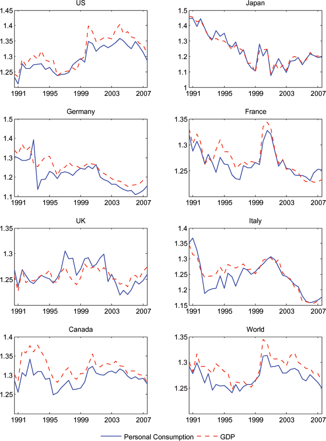
Figure 3:  Expected Personal Consumption Growth and Expected Real Interest Rate

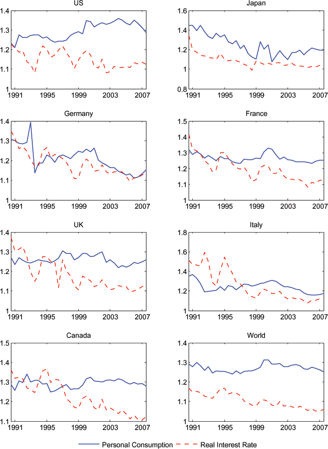
Figure 4:  Coefficients on Expected GDP Growth and Expected Real Interest Rate (Baseline Specification)

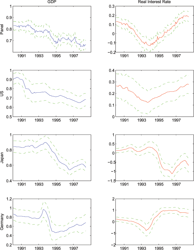
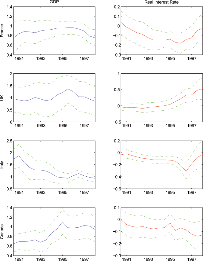
Figure 5:  Coefficients on Expected GDP Growth and Expected Real Interest Rate (Specification with Variables as a Ratio to World Consumption)

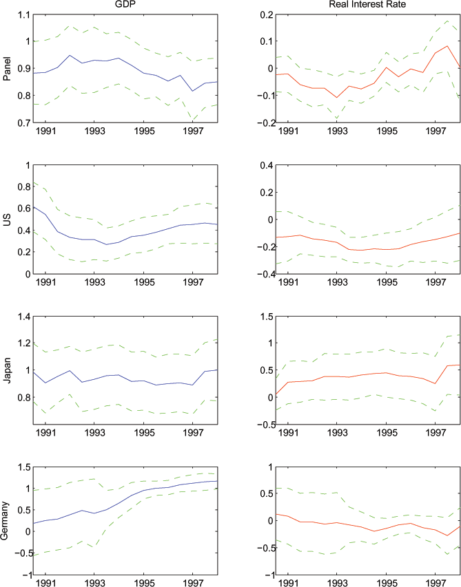
Note: As in Figure 4, with estimates from equation (7).

Figure 6:  Coefficients on Expected GDP Growth and Expected Real Interest Rate (Specification with Natural Log of Variables)

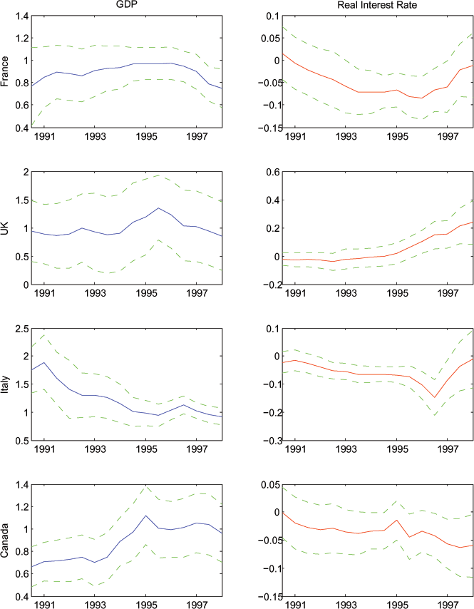
Note: As in Figure 4, with variables now in logs.

Figure 7:  Coefficients on Expected GDP Growth and Expected Real Interest Rate (Specification with Natural Log of Variables as a Ratio to World Consumption)

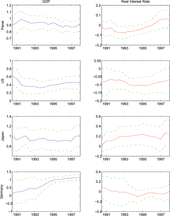
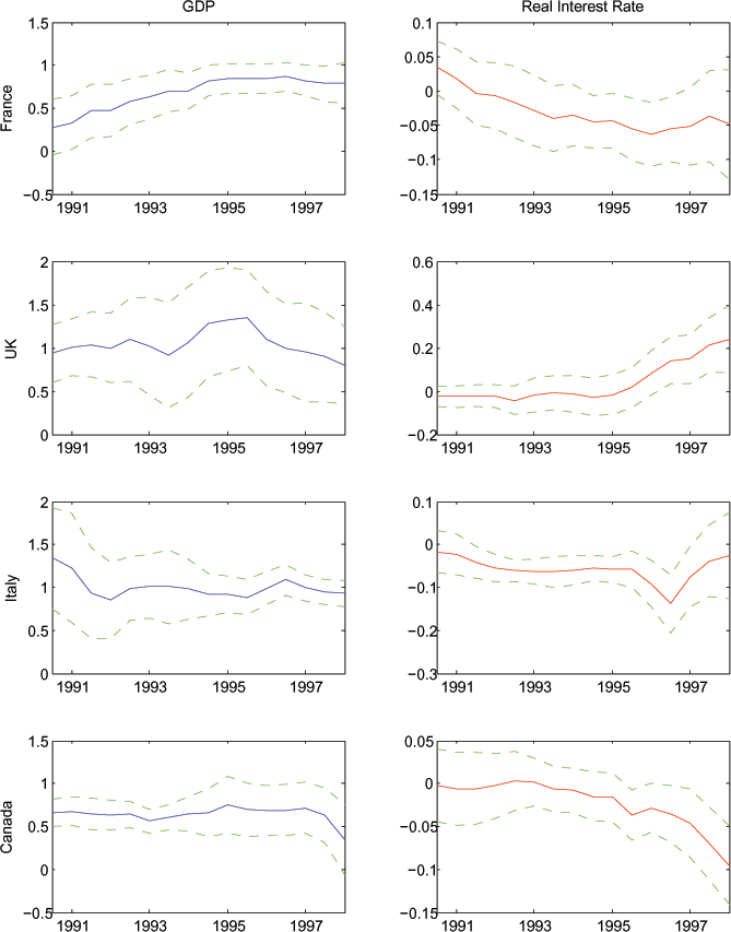
Note: As in Figure 5, with variables now in logs.

Figure 8:  Coefficients on Expected GDP Growth, Expected Real Interest Rate, and World Consumption (Specification with Natural Log of Variables)

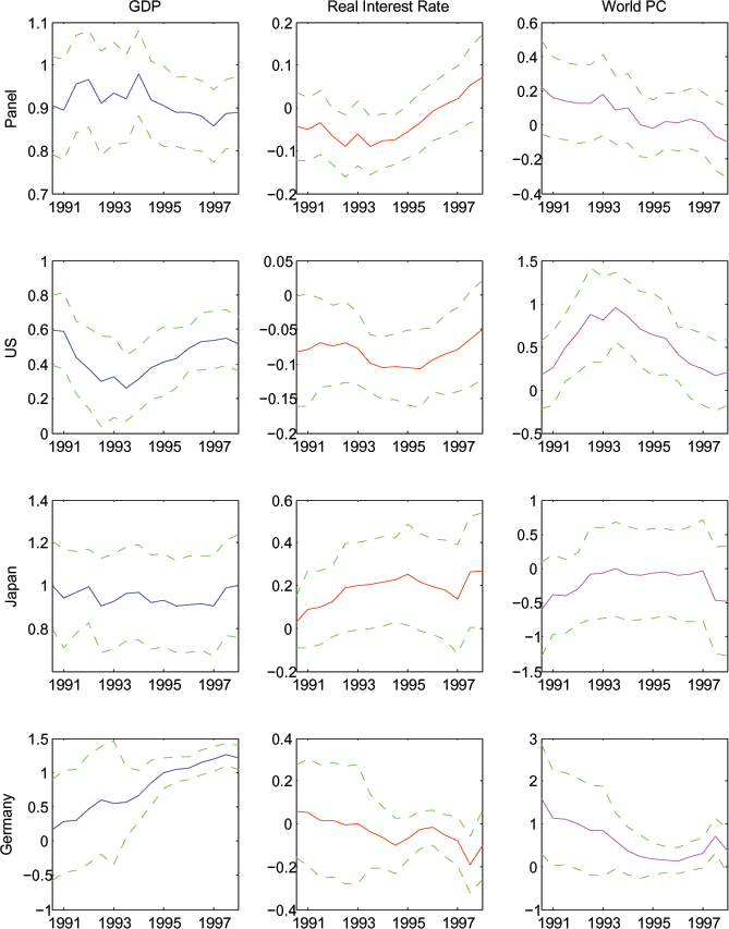
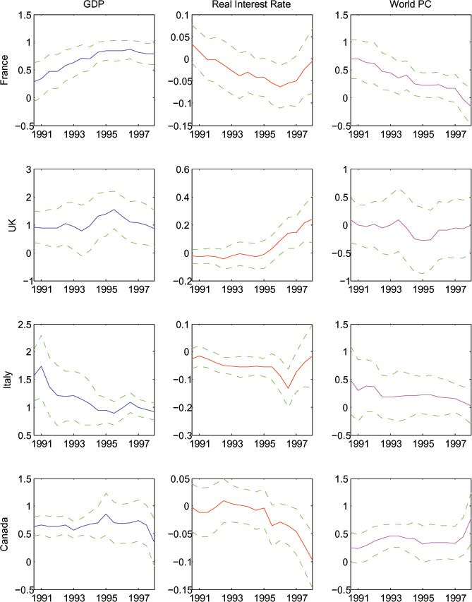
Note: As in Figure 6, adding log world consumption as a regressor.

Figure A1:  Expected Personal Consumption Growth

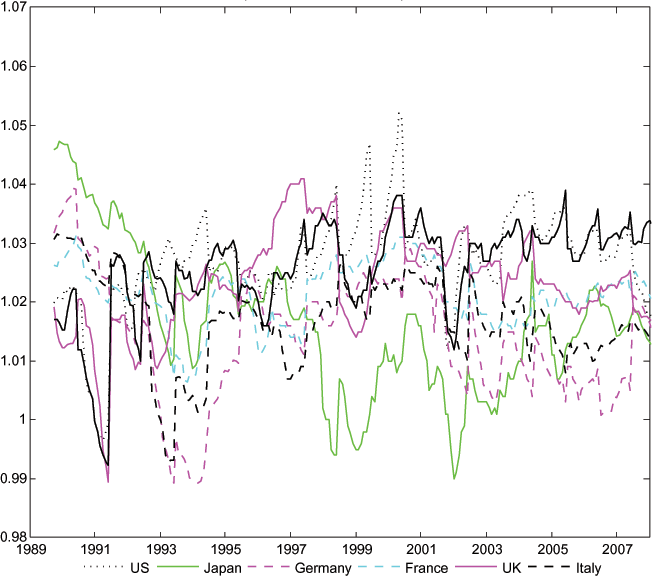
Note: As in Figure 1, with one year expectations.

Figure A2:  Expected Personal Consumption Growth and Expected GDP Growth

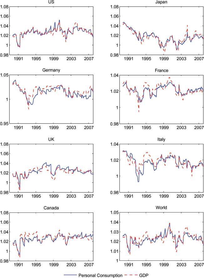
Note: As in Figure 2, with one year expectations.

Figure A3:  Expected Personal Consumption Growth and Expected Real Interest Rate

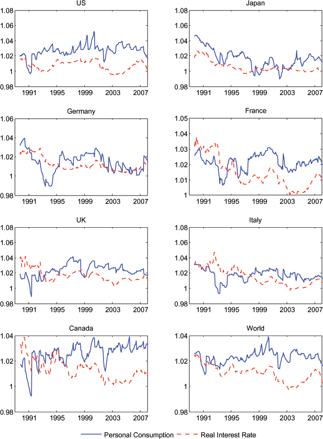
Note: As in Figure 3, with one year expectations.

Figure A4:  Coefficients on Expected GDP Growth and Expected Real Interest Rate (Specification with Natural Log of Variables

Note: As in Figure 6, with one year expectations.

Footnotes

*  Author notes: Engel is Professor of Economics at the University of Wisconsin.  He can be reached at [email protected]. Rogers is Deputy Associate Director in the Division of International Finance of the Federal Reserve Board, and can be reached at [email protected].  We thank Ben Chiquoine for outstanding research assistance and Andrea Ferrero and Robert Kollmann for comments.  The views in this paper are solely the responsibility of the authors and should not be interpreted as reflecting the views of the Board of Governors of the Federal Reserve System or of any other person associated with the Federal Reserve System. Return to text

1.  Engel and Rogers (2006) provide evidence in favor of a modified version of the present-value model to explain the U.S. current account deficit. That study makes use of the long-run forecasts of GDP used in the current paper. However, that paper does not use the forecasts of consumption used in this study, and it appears that those forecasts may not be consistent with some of the underlying equations in Engel and Rogers (2006). That paper, in essence, assumes that differences in expected consumption growth across countries can be attributed to expected real exchange rate changes. Return to text

2.  As section 3 below details, we treat the April and October surveys slightly differently. The April measure of expected consumption includes the forecast of the current year expected growth rate in the 10-year average, but for the October measure we measure the 10-year forecasted growth rate using the survey measure of the expected growth rate in the upcoming year and the next 9 years. For robustness we also examine the survey expectations at the one year ahead horizon. Return to text

3.  This mechanism is present in Bergin and Sheffrin's (2000) study of the present-value model. They consider a model with non-traded goods, so overall price levels are not equalized across countries. Real exchange rate changes play an important role in their test of the PVM. Return to text

4.  It is important to realize that this is not simply a necessary outcome of national income accounting: Y = C + I + G + NX. The whole point of the present-value model of the current account is that well-functioning international capital markets break the link between current income and consumption. The difference gets reflected in the current account. Return to text

5.  Note that the panel of forecasters is not identical across the G-7 countries nor across time. However, many panelists do provide forecasts for several countries. Furthermore, although participants do come in and out of the survey this does not occur very often. Response rates are in general very high, (close to 100%), but can be somewhat smaller for the long-horizon forecasts and/or for some of the smaller countries. Return to text

6.  This is similar to one of the regressions run by Campbell and Mankiw (1987) who use actual (U.S.) data, rather than forecasts Return to text

7.  The weight applied to any country's growth rate is essentially that country's share of G7 real GDP. As in our earlier paper (Engel-Rogers, 2006) we use 1990 real exchange rates to convert nominal GDP shares to real shares; see that paper for more details. Return to text

8.  See Backus and Smith (1993) for an early formulation of the problem. Corsetti, Dedola, and Leduc (2008) is a recent paper that addresses the puzzle. Return to text

9.  There is of course a long literature evaluating various properties of survey responses of professional forecasters. Much of this work has evaluated the survey forecasts of inflation. In two recent such contributions, Ang, Bekaert, and Wei (2007) and Croushore (2007) present quite favorable evidence on the properties of the survey forecasts. These recent papers argue that earlier papers that had found strong evidence against the rationality of survey forecasts were ignoring real-time issues, putting too much weight on the time around 1980 when there was learning about structural breaks, and not doing the econometrics of relationships among highly persistent variables correctly. The evidence on post-1985 data that is more careful on econometrics and real-time issues doesn't find a whole lot of evidence of substantive deviations from forecast efficiency. As noted, this work has all focused on inflation forecasts; we are not aware of a comparable literature evaluating the properties of the long-horizon forecasts of consumption that we use in this paper. Return to text

10.  Recent examples include Caballero, Farhi, and Gourinchas (2008) and Ferrero (2007). Return to text

This version is optimized for use by screen readers. Descriptions for all mathematical expressions are provided in LaTex format. A printable pdf version is available. Return to text

Home | Economic research and data | Publications and education resources
Accessibility | Contact us
Last update: September 26, 2008