Skip to: [Printable Version (PDF)]

Board of Governors of the Federal Reserve System
International Finance Discussion Papers
Number 987, December 2009 --- Screen Reader Version*

Are Chinese Exports Sensitive to Changes in the Exchange Rate?

Shaghil Ahmed¹

NOTE: International Finance Discussion Papers are preliminary materials circulated to stimulate discussion and critical comment. References in publications to International Finance Discussion Papers (other than an acknowledgment that the writer has had access to unpublished material) should be cleared with the author or authors. Recent IFDPs are available on the Web at http://www.federalreserve.gov/pubs/ifdp/. This paper can be downloaded without charge from the Social Science Research Network electronic library at http://www.ssrn.com/.

Abstract:

This paper builds a model of two types of Chinese exports, those processed and assembled laregely from imported inputs ("processed" exports) and "non-processed" exports. Based on this model, the sensitivity of Chinese exports to exchange rate changes is empirically examined. Unlike previous work, the estimation period includes the net real appreciation of the renminbi that has occurred over the past three years. The results show that greater exchange rate appreciation dampens export growth, both for non-processed and processed exports, with the estimated cumulative price elasticity being substantially greater than unity. When the source of the increase in the Chinese real exchange rate is appreciations against the currencies of other emerging Asian trading partners, the effect on processing exports is positive but insignficant, while the effect on non-processing exports is significantly negative. By contrast, when the source of the increase in the Chinese real exchange rate is appreciation against China's advanced-economy trading partners, the effects on both types of exports are negative. These results are consistent with the predictions of the theoretical model. Counterfactual simulations based on the estimated model strongly suggest that if the trade-weighted real renminbi had appreciated at an annual rate of 10 percent per quarter since mid-2005, Chinese real exports would have been roughly 30 percent lower today. Thus greater exchange rate flexibility could contribute to lowering China's huge trade surplus through restraining growth of exports.

Keywords: China, exchange rate, exports

JEL classification: F31, F32, F41

1  Introduction

China's ballooning current account surplus in recent years (reaching about 10 percent of GDP in 2008) and rapid accumulation of international reserves (to about $2.2 trillion) has raised concerns that Chinese authorities are heavily managing their currency and contributing to global imbalances. At the same time, many also question whether faster currency appreciation would reduce China's trade surplus significantly-one argument being that, given the high import content of Chinese exports, appreciation of the currency need not make Chinese exports more expensive to the rest of the world since the effective cost of the imported inputs would also fall. Despite this tension there is relatively little empirical evidence on how responsive Chinese exports have, in fact, been to currency movements that cover the period since the middle of 2005 when China revalued the renminbi (RMB) and started allowing a moderate appreciation trend, at least until the middle of last year.

This paper provides empirical estimates of the sensitivity of Chinese exports to exchange rate changes. It distinguishes between the effects on "processed" exports (produced using parts and components imported from abroad) and "non-processed" exports (largely sourced from domestic inputs). It also attempts to distinguish between unilateral changes in the Chinese exchange rate and those that are highly correlated with exchange rate changes of other economies in the region from which China imports parts and components, since this distinction is potentially very important when both processed and non-processed exports are being produced.

There are some existing empirical studies that also distinguish between processed and non-processed Chinese exports-Aziz and Li (2007), Cheung, Chinn and Fujii (2008), Garcia-Herero and Koivu (2009), Marquez and Schindler (2007), and Thorbecke and Smith (2008)-and Thorbecke and Smith also consider unilateral versus multilateral (across Asia) real effective exchange rate changes. However, only two of these studies incorporate any part of the period since mid-2005 in their sample period, and none of them consider the period from 2007 to mid-2008, when the pace of appreciation of the RMB apparently was accelerated. All told, the trade-weighted Chinese real exchange rate has appreciated about 13 percent, on net, since the end of 2006. Taking account of the greater recent variability of the exchange rate, this study provides up-to-date estimates and compares these to earlier estimates. Given concerns about possible currency undervaluation it also uses simulations from the empirical model to examine what the behavior of Chinese exports might have been if the RMB had appreciated more in recent years.

Another key distinguishing characteristic of this paper is that it develops a theoretical model of Chinese exports that explicitly incorporates the import of inputs for the production of some types of exports goods. This means that the estimated equations for exports are well-grounded in economic theory, including predictions about the different effects of RMB appreciation when its source is movements against the currencies of other emerging Asian economies and when its source is movements against the currencies of China's other trading partners. The explicit derivation of reduced-form export equations from theory also makes it clear that the estimated relative price elasticity should not be viewed, as it often is, as the slope of the demand curve, and the income elasticity should not be viewed as representing how much the demand curve shifts in response to a change in income, as the equilibrium quantities will incorporate supply-side parameters as well.

The main results of the paper can be summarized as follows: First, including the latest period of greater real exchange rate variability reinforces the conclusions of some earlier studies, such as Marquez and Schindler (2007), which found that Chinese exports respond quite strongly to movements in the real exchange rate, and go against studies which find little effect of exchange rate changes or effects that go in the opposite direction to conventional wisdom. Second, considering the components of the real exchange rate, consistent with the theoretical model, when the source of Chinese real exchange rate appreciation is movements of the RMB against other emerging Asian countries, this does not have a significant effect on Chinese processing exports, but it does have a significant negative effect on Chinese non-processing exports. On the other hand, when the source of the renminbi appreciation is movements against the currencies of non-emerging Asian Chinese trading partners, generally both types of exports go down. Moreover, even though processed exports remain very important for China, increases in non-processed exports have recently accounted for more of the overall increase in exports. Finally, model simulations indicate that the path of total Chinese real exports would have been quite a bit lower if the renminbi had appreciated more in recent years.

Overall, the results suggest that greater exchange rate flexibility could have significant impact on China's trade balance by restraining growth of exports, particularly non-processed exports.

The remainder of the paper is organized as follows. Section 2 sets the scene by discussing key developments in the Chinese external sector in recent years and Section 3 provides a selective review of the existing empirical work in this area. Section 4 presents a simple theoretical model of the behavior of Chinese exports that forms the basis of the empirical specification used. The empirical results on the exchange rate sensitivity of Chinese exports are presented and discussed in Section 5. Section 6 concludes.

2  Background: Developments in the Chinese External Sector

When discussing global imbalances, one of the key developments often referred to is the phenomenal rise in China's external surpluses since China's entry into the WTO in December 2001. As can be seen from Figure 1, China's current account surplus increased from a relatively modest under 2 percent of GDP ($17 billion) in 2001 to 11 percent of GDP in 2007, before falling a bit to a still-high of just under 10 percent of GDP last year ($430 billion). The ballooning surplus in recent years has raised concerns among some international analysts that China has been following a mercantilist approach and keeping its currency artificially (and some argue unfairly) undervalued to pursue an export-led growth strategy. In the first half of 2009, though, the Chinese current account surplus narrowed sharply, to 6.5 percent of GDP, as the global crisis led to Chinese exports falling much more than Chinese imports. (Chinese balance of payments (BOP) data are reported only semi-annually.)

Of course, a large trade surplus, just by itself does not necessarily imply intervention in exchange markets. But accompanying the phenomenal rise in the Chinese current account surplus in recent years has been an even more phenomenal rise in China's international reserves, from about $200 billion in 2001 to $2 trillion at the end of 2008-this year, reserves have risen further to about $2.2 trillion (see Figure 2), despite the narrowing of the current account surplus. There are many good reasons for emerging market economies (EMEs) to build up a war chest of reserves for insurance purposes against crisis situations, and the relatively high level of international reserves compared to past crises helped the EMEs cope better during the recent global crisis. Nevertheless, the sheer magnitude of China's reserve accumulation has led to questions about the possibility of an undervalued exchange rate.

How has the exchange rate itself behaved? This is shown in Figure 3. As can be seen from the thick black line, Chinese authorities maintained a dollar peg until the middle of 2005. After a one-time appreciation of about 2 percent of the RMB against the dollar, Chinese authorities allowed further gradual appreciation until about the middle of last year. Since that time, the RMB appears again to have been de facto pegged against the dollar. On net, the nominal value of the RMB against the dollar has declined roughly 25 percent since mid-2005.

The trade-weighted real and nominal effective exchange rates are shown by the blue dashed and red dotted lines, respectively, in Figure 3. Note that the trade-weighted effective exchange rates vary more than the bilateral rate against the dollar. Even over the period when the value of the RMB was pegged, in effective terms (both real and nominal), the exchange rate was varying. At first, it followed a generally appreciating trend until the end of 2001 and then a generally depreciating one until mid-2005. After the peg was dismantled, there was a generally appreciating trend of the effective exchange rates until about the end of last year, especially toward the end of that period with the RMB/Dollar rate constant and the dollar appreciating sharply against other major currencies. This year, the real effective exchange rate has moved down, reflecting dollar weakness against other major currencies and a continued fixed RMB against the dollar. The cumulative appreciation of the Chinese real exchange rate since June 2005 has been about 13 percent.

Two other scene-setting developments are useful to note. The first relates to speculative activity based upon anticipations of the future behavior of the RMB. Figure 4 gives the sources of the change in international reserves, decomposing these changes into what can be accounted for by the trade balance, net foreign direct investment (FDI) inflows, and the remainder-what people have often called "hot money" inflows (measured as the residual).² Note that in 2004, speculation was rife about the abandoning of the peg against the dollar and only less than half of the change in international reserves could be accounted for by the trade surplus (the green bar) and net FDI (the blue bar). Hot money inflows (the red bar) were thus large, given expectations of appreciation of the RMB, which did become partly fulfilled in mid-2005. Hot money net flows since then appear to have been more modest, with a small net outflow last year and a somewhat bigger one in the first half of this year. In recent months, however, although we cannot provide an actual estimate, since Chinese BOP data are only semi-annual, the sharp narrowing of the trade balance together with the acceleration in the pace of reserves accumulation suggests that hot money inflows have picked up again.

The second important development is the different behavior of processing and non-processing trade. Much of China's trade involves importing inputs and parts and components with very little import duties (imports for processing) and adding value through processing and assembly of these parts and components into goods that are then re-exported (processed exports). The processed exports have a much higher import content than non-processed exports.³ Chinese customs records keep a distinction between "processing" and non-processing trade, labelling the latter as "ordinary" imports and exports.

The seasonally-adjusted (using X-12) quarterly nominal values of processing and non-processing exports and imports are shown in Figures 5 and 6. Each type of export constitutes about half of total exports. Several features are noteworthy. First, processing goods exports and imports grow and fall together. Second, over the better part of the last decade, including this year, China ran a deficit on non-processing trade, which implies that the surplus on processing trade was larger than China's overall trade surplus. Third, before the global crisis hit, non-processing exports were rising at a higher pace than processing exports and contributing more to export growth. More recently, non-processing imports have picked up again after the collapse of trade during the crisis, but non-processing exports have not yet shown a similar pickup, which has been a big source of the recent narrowing of China's overall trade surplus. The distinction between processed and non-processed exports-and their different behaviors-is important for the question of looking at the effects of exchange rate changes, because with a high import content, processed exports may be less responsive to changes in the Chinese exchange rate against the currencies of those countries it imports inputs and parts and components from.

3  Review of Previous Empirical Work

The extent of the possible undervaluation of the Chinese exchange rate has been the subject of intense debate in recent years. Cline and Williamson (2008) provide a survey of the range of estimates. Leaving aside a few outliers, the typical range of the degree of undervaluation of the Chinese real effective exchange rate is 8 percent to 55 percent. The average undervaluation for studies dated 2005 or afterwards is 26 percent.⁴ The estimates differ because of the approach taken as well as differences in assumptions that are made within a given approach. Despite these estimates, some continue to argue, along the lines of Mundell (2004), that China should not be pressured to appreciate its currency substantially, as this, among other things, would undermine its growth miracle.

The approaches used to estimate the extent of the undervaluation are also discussed by Cline and Williamson as well as by Dunaway, Leigh, and Li (2009). One of the key approaches is the macroeconomic balance approach, which typically involves first computing the long-run sustainable equilibrium current account balance and then the change in the real exchange rate that would be required to close the gap between the actual current account balance and this equilibrium value.^{5, 6} Obviously, in computing the change in the real exchange rate required using this approach, assumptions will have to be made about the relative price elasticities of exports and imports. Studies using this approach for China do not always carefully justify the choice of trade elasticities or explicitly lay out the trade models (theoretical or empirical) that are the sources of these choices.

It will, therefore, be useful to review what the existing empirical literature says about the sensitivity of Chinese trade to changes in the exchange rate. Since the focus of this paper is on exports, attention is confined here to estimates of export elasticities.

Studies of export effects of exchange rate changes using earlier data, such as Cerra and Dayal-Gulati (1999), Cerra and Saxena (2003), and Eckaus (2004) do not find consistent or stable estimates. As Marquez and Schindler (2007) have argued, the estimates of these earlier studies cannot be relied upon, partly because they include a period of transformation from a centrally-planned economy to a market-oriented system and because they include periods in which there was little movement in the nominal exchange rate and little movement in the real effective exchange rate as well.

Another important criticism that Marquez and Schindler level against much of the work in the area of estimating trade elasticities for China is that since Chinese trade prices are not available, studies use imperfect proxies for these prices, including using trade price data from China's trading partners, especially Hong Kong. To avoid distorting the results, these authors conduct their own very comprehensive analysis that is based on studying nominal shares of Chinese trade in world trade, modeling these shares as depending on economic activity and the real exchange rate. Focusing on these nominal shares does not require them to take a stand on which proxy to use for trade prices.

Their results are widely-cited. Using monthly data from 1997-2004, they find that for non-processed exports, a 10 percent appreciation of the RMB would decrease the world share of Chinese exports by about a half percentage point in the long run, which is a fairly big effect. The results for processed exports are less clear-cut and sensitive to the lag length used in the estimated equations.

The point made by Marquez and Schindler about proxies for Chinese trade prices being imperfect is well-taken. However, as they acknowledge, a drawback of their procedure is that the price responsiveness of trade volumes is not identified. But some idea of this price responsiveness is very important in one of the key approaches to obtaining the degree of RMB misalignment and informing the debate in this area. Over time, the criticism raised by Marquez and Schindler may have become less important as the U.S. has maintained, since 2003, a Chinese import deflator, which may actually be a reasonably good proxy for the overall price deflator for Chinese exports.

Recent studies that use proxies for Chinese trade prices include Aziz and Li (2007) and Cheung et al (2009). Aziz and Li, using quarterly data from 1995-2006 find an aggregate export price elasticity with respect to RMB real appreciation of about -1 1/2, and disaggregated elasticities of about -2 1/4 for non-processed exports and about -1/2 for processed exports.⁷ These elasticities are statistically significant.⁸ Using rolling regressions, they also find that, while the elasticity for non-processed exports has stayed relatively constant, the elasticity for processed exports first decreased and then (in samples that include the period since mid-2005) increased.⁹ For their latest sub-sample of 1999-2006, the price elasticity of processing exports is about -1.4.

Cheung et al use a similar empirical specification based on a sample period that generally uses quarterly data over the period 1993:3-2006:2. However, they obtain quite different results. Their specification for exports includes a foreign activity variable, a real exchange rate variable, and a supply-shift variable, measured as the capital stock in manufacturing. They find that, although real exchange rate appreciation lowers exports as expected a priori, the effect is not statistically significant. The income effects are also not generally significant, although the capital stock always has a significantly positive effect on exports. They also consider a specification that excludes the capital stock, but this results in estimates that are very counterintuitive-exchange rate appreciations in this case have a significantly positive effect on both non-processing and processing exports. The authors conclude that Chinese export price elasticities are not very precisely determined.¹⁰

Another very recent study is Garcia-Herrero and Koivu (2009). However, the sample period they used in their research only goes up to the end of 2005. The effects of relative price increases are in the expected direction. For non-processing exports, they find a long-run relative price elasticity of -2.3 for the full sample period of 1994-2005, but a lower elasticity of -1.6 for the more recent sub-sample 2000-2005.¹¹ For processed exports, the long-run price elasticity is around -1.3 for both sample periods.¹²

A carefully done study that emphasizes the central importance of unilateral RMB changes versus multilateral ones (that are accompanied by similar movements in the exchange rates of other Asian economies against the currencies of their Western trading partners) is Thorbecke and Smith (2008).¹³ They use an annual panel data set over the period 1992-2005 to model Chinese bilateral real exports (both processing and non-processing) to 33 countries.¹⁴ The standard foreign output and bilateral real exchange ($rer$) rate variables are included in the specification for non-processing exports. For processing exports, account is taken of how the bilateral real exchange rates of a trading partner with other countries that China imports inputs from would affect Chinese imported input prices. Specifically, the relative price variable in the bilateral processing exports equation for trading partner $i$ is an integrated real exchange rate ($irer$), which is a weighted average of the $rer$ and the average real exchange rate of the other countries in Asia (from which China imports the bulk of parts and components) with trading partner $i$ ($wrer$). The weight attached to $rer$ in the computation of $irer$ is the share of valued added by China in total processing exports and the weight of $wrer$ is 1 minus that.

This is a very interesting approach that also yields interesting empirical results. The authors results imply that if only the RMB appreciated, say a 10 percent rise in $rer$ with $wrer$ unchanged, processing exports would fall by 4 percent only (a price elasticity of -0.4). If, however, all of the currencies in emerging Asia appreciated against other currencies along with the RMB (a 10 percent rise in both $rer$ and $wrer$), then processing exports fall by much more (10 percent, or an elasticity of -1). Intuitively, this holds because when $wrer$ is unchanged, this means the RMB is appreciating against its other emerging Asian trading partners also, which means imported inputs become cheaper, partially offsetting the negative effect on processing exports.¹⁵ Since processing exports, being more sophisticated, are the ones that European and U.S. goods could be potential substitutes for, the authors argue that only general exchange rate adjustment throughout emerging Asia would do something for global imbalance adjustment.

While this approach is interesting and informative, it does not address some issues. First it implicitly assumes that the share of value-added in total processing exports is exogenously given and not itself affected by the relative prices. Second, the specifications using bilateral trade and bilateral real exchange rates do not allow for third-party competition effects so that the equations might be misspecified. Third, from the viewpoint of the demanders of the final processed export goods, e.g. U.S. consumers, only the relative price of the final good should matter; the distinction between what is happening to the RMB versus other Asian currencies is relevant for the supply-side of processing exports only, and should focus directly on RMB movements against these currencies rather than indirect movements of these currencies against particular trading partners, such as the U.S. The approach taken in this paper is different, but complementary, and is grounded in a theoretical model that derives the demand and supply functions of processing and non-processing exports explicitly.

As mentioned before, none of the empirical studies discussed above includes the period since the end of 2006-a period over which interesting and new developments have taken place in the Chinese external sector-as part of the sample period. In particular, the greater variability in the real exchange rate observed over this period should give more precise estimates.¹⁶

4  Modeling Chinese Exports: Theory

In this section, the demand and supply of Chinese exports are derived theoretically and market-clearing conditions used to obtain equations for the equilibrium growth rates of Chinese exports that form the basis of the empirical work. The estimated equations will allow more dynamics than is embedded in the simple theoretical model.

4.1  Demand for Chinese Exports

Importers of Chinese goods from the rest of the world are assumed to consume three types of goods: a Chinese good that is produced largely from inputs and components that are imported into China and then assembled into final products in China for export ($M_{A}$)--what we have been calling processed exports; a Chinese export good that relies more heavily on inputs produced in China, i.e. domestically sourced ($M_{D}$)--what we have been calling non-processed exports; and an aggregate of all other goods consumed by the rest of the world, including goods they produce domestically and import from other countries ($C_{O}$). The preferences of the rest of the world consumers for these three types of goods are given by a CES utility function:

$$u(M_{A},M_{D},C_{O})=\left[ \phi_{A}^{1/\sigma}M_{A}^{\frac{\sigma-1}{\sigma }}+\ \phi_{D}^{1/\sigma}M_{D}^{\frac{\sigma-1}{\sigma}}+(1-\phi_{A}-\phi _{D})^{\frac{1}{\sigma}}C_{O}^{\frac{\sigma-1}{\sigma}}\right] ^{\frac {\sigma}{1-\sigma}}$$ (1)

where $\sigma~$is the elasticity of substitution, and the $\phi$'s are preference parameters. The division of aggregate consumption expenditure by the rest of the world on the three goods they consume can be written as:

$$P_{A}^{\ast}M_{A}+P_{D}^{\ast}M_{D}+P_{O}^{\ast}C_{O}=P_{C}^{\ast}C^{\ast}$$ (2)

where the $P^{\ast}$'s represent foreign prices and $P_{C}^{\ast}$ is the aggregate foreign consumer price (CPI) and $C^{\ast}$ is aggregate real foreign consumption. The first order necessary conditions of maximizing (1) subject to (2) give rise to the following standard demand functions:

$$M_{A}=\phi_{A}\left( \frac{P_{A}^{\ast}}{P_{C}^{\ast}}\right) ^{-\sigma }C^{\ast}$$ (3)

$$M_{D}=\phi_{D}\left( \frac{P_{D}^{\ast}}{P_{C}^{\ast}}\right) ^{-\sigma }C^{\ast}$$ (4)

$$C_{O}=(1-\phi_{A}-\phi_{D})\left( \frac{P_{O}^{\ast}}{P_{C}^{\ast}}\right) ^{-\sigma}C^{\ast}$$ (5)

where the aggregate foreign CPI is defined as:

$$P_{C}^{\ast}=\left[ \phi_{A}P_{A}^{\ast^{1-\sigma}}+\ \phi_{A}P_{D} ^{\ast^{1-\sigma}}+(1-\phi_{A}-\phi_{D})P_{O}^{\ast^{1-\sigma}}\right] ^{\frac{1}{1-\sigma}}$$ (6)

Looking a bit ahead, the real exchange rate is going to be assumed to be a policy variable that Chinese authorities will target. Accordingly, it will be useful to rewrite the demand functions (3) and (4) in terms of the real trade-weighted CPI-based Chinese real exchange rate and the local currency prices of the Chinese export goods. Define the real exchange rate to be:

$$Q=\frac{EP_{C}}{P_{C}^{\ast}}=(Q_{A}^{\prime})^{\varpi}(Q_{B}^{\prime })^{1-\varpi}=Q_{A}Q_{B}$$ (7)

where $E$ is the nominal trade-weighted Chinese exchange rate, expressed as foreign currency per unit of the RMB, and $P_{C}$ is the Chinese aggregate CPI. Note that a rise in $Q$ represents a real exchange rate appreciation for China. The aggregate real exchange rate index, $Q$, is decomposed into components attributable to China's trading partners in the rest of emerging Asia, $Q_{A}$, and China's other trading partners, $Q_{B}$, with $Q_{A}^{\prime},$ $Q_{B}^{\prime}\$being the component real exchange rates and $\varpi$ and $1-\varpi$ being the weights attached to the two sets of countries, respectively, in the aggregate real exchange rate index. This distinction will be useful when we consider the supply of Chinese exports. Equation (7) can be used to rewrite (3) and (4) as:

$$M_{A}=\phi_{A}Q^{-\sigma}\left( \frac{P_{A}}{P_{C}}\right) ^{-\sigma} C^{\ast}$$ (8)

$$M_{D}=\phi_{D}Q^{-\sigma}\left( \frac{P_{D}}{P_{C}}\right) ^{-\sigma} C^{\ast}$$ (9)

where $P_{A},P_{D}$ represent the domestic currency (RMB) prices of the goods, and purchasing power parity for traded goods is being assumed. In the empirical work, we will use growth rates of the variables to ensure stationarity. Equations (8) and (9) in growth-rate form can be approximated by taking logs and first-differencing to yield:

$$\Delta m_{A}=-\sigma\left[ \Delta q+\Delta(p_{A}-p_{C})\right] +\Delta c^{\ast}$$ (10)

$$\Delta m_{D}=-\sigma\left[ \Delta q+\Delta(p_{D}-p_{C})\right] +\Delta c^{\ast}$$ (11)

where lower case letters represent the natural logarithm of a variable, and $\Delta$ is the first difference operator. Note that the elasticity with respect to foreign consumption is unity because of the choice of CES utility function. However, in the empirical work we will be estimating reduced forms that allow for this elasticity to differ from unity if the data so dictate.

4.2  Supply of Chinese Exports

Three goods are produced in China: a non-traded aggregate good and the two export goods whose demand was discussed above. The aggregate non-traded good is assumed to be the only consumption good in the economy. The supply of the three goods is subject to Cobb-Douglas technology:

$$X_{C}=A_{C}L_{C}^{\alpha_{C}}K_{C}^{1-\alpha_{C}}\exp\{\eta_{C}\}$$ (12)

$$X_{D}=A_{D}L_{D}^{\alpha_{D}}K_{D}^{1-\alpha_{D}}\exp\{\eta_{D}\}$$ (13)

$$X_{A}=A_{A}L_{A}^{\alpha_{A}}Z^{\alpha_{Z}}K_{A}^{1-\alpha_{A}-\alpha_{Z}} \exp\{\eta_{A}\}$$ (14)

where $X_{C}$ is the supply of the Chinese non-traded (consumption) good, $X_{D}$ is the supply of the Chinese export good using only domestic inputs, $X_{A}$ is the supply of the Chinese "assembled" export good, the $A$'s represent the state of technology, the $L$'s and the $K$'s represent labor and capital, respectively, allocated to the various sectors, $Z$ represents the imports of inputs, parts, and components from abroad, and the $\eta$'s represent the technological innovations to the different sectors.¹⁷

Firms are assumed to choose their demand for labor and their demand for the imported input based on profit maximization. However, in the case of China, it is highly debatable to what extent the quantity of capital and its allocation across sectors is determined by profit-maximizing behavior in response to changes in interest rates and their effects on the user cost of capital. The government has quite a substantial degree of influence through directed lending and informal assigned lending quotas (the so-called "window guidance") as well as through state approval of investment projects. In light of this, we assume the stock of capital and its allocation across sectors to be determined outside the model.

Profit maximization yields the following standard labor demand functions and the imported input demand function that follow from the Cobb-Douglas technology:

$$\alpha_{i}\frac{X_{i}}{L_{i}}=\frac{W}{P_{i}}\ \ \ \ \ \ \ \$$ (15)

for $i=C,D,A,$ respectively.

$$\alpha_{Z}\frac{X_{A}}{Z^{d}}=\frac{P_{Z}}{P_{A}}$$ (16)

where $W$ is the economy-wide wage rate, $Z^{d}$ is the demand for the imported input, $P_{Z}$ is the local currency (RMB) price of the imported input, and $L_{C},L_{D},L_{A}$ are the quantities of labor demand in the three sectors. For simplicity, labor is assumed to be elastically supplied at a fixed economy-wide real wage rate, measured in consumption units.¹⁸ Specifically,

$$W=\mu P_{C}$$ (17)

Other countries in emerging Asia are assumed to supply the input $Z$ to China. The supply of this input is assumed to be price elastic and given by:

$$Z^{s}=\left( \frac{P_{Z}^{\prime}}{P_{C}^{\prime}}\right) ^{\gamma}B=\left( \frac{Q_{A}^{\prime}P_{Z}}{P_{C}}\right) ^{\gamma}B$$ (18)

where $B$ is the scale factor for the input supply, $P_{z}^{\prime}$ is the foreign (Asian) currency price of the input exported by rest of emerging Asia to China, $P_{C}^{\prime}$ is the domestic price of the aggregate consumption good in the input-exporting countries, and purchasing power parity for traded goods is assumed to hold, so that $E^{\prime}P_{Z}=P_{Z}^{\prime}$ where $E^{\prime}$is the nominal exchange rate expressed as units of foreign Asian currency per RMB. Recall that $Q_{A}^{\prime}$ is the CPI-based real exchange rate of China vis-a-vis other emerging Asian countries, which are the countries China is assumed to imports its inputs and parts and components from:¹⁹

$$Q_{A}^{\prime}=\frac{E^{\prime}P_{c}}{P_{C}^{\prime}}$$ (19)

For a given Chinese currency price of the input $P_{Z}$, a rise in $Q_{A}^{\prime}$ means foreigners supplying the input would receive more for it, increasing the supply of it, as can be seen from (18). An alternative equivalent way to characterize the situation is that for a given foreign currency price of the input $P_{Z}^{\prime}$, a rise in $Q_{A}^{\prime}$ means less would have to be paid for a given amount of the input by the Chinese in RMB, thus increasing the demand for the input. Viewed either way, whether we think of the demand and supply curves for the imported input being drawn in $P$ or $P_{Z}^{\prime}$ space, the equilibrium quantity of the imported input would rise following a real RMB appreciation against the other emerging Asian currencies.

To derive, in growth rate terms, the supply functions of the two goods that China exports, the growth rate of the equilibrium quantity of the imported input for any given level of production of the export good ($X_{A}$) that uses this input is first derived. This is done by taking logs of equations (16) and (18), first differencing and then equating growth of the demand for the input to the supply of the input to solve for the price level change $\Delta p_{Z}$, which is then substituted back into either the growth of demand or the growth of supply of the input to yield:

$$\Delta z=\frac{1+\gamma(1-\mu_{Z})}{1+\gamma}+\frac{1}{1+\gamma}\Delta q_{A}^{\prime}+\frac{1}{1+\gamma}\Delta(p_{A}-p_{C})+\frac{\gamma}{1+\gamma }\Delta x_{A}\$$ (20)

where recall that lower case letters represent logs, $\Delta$ represents the first-difference, $\mu_{Z}$ is the long-term growth of the supply shift factor $B$ in (18). As discussed above, $\Delta q_{A}^{\prime}>0$ would increase the equilibrium quantity of the imported input. Rises in $x_{A}$ and $p_{A}$ represent positive shifts to the demand for the input and raise equilibrium imports of the input. As to the effect of $p_{c}$, for a given real exchange rate $q_{A}^{\prime}$, a rise in $p_{C}$ will mean a higher $p_{c}^{\prime}$ and/or a lower $e^{\prime}$. In either case, the relative price facing local suppliers would go down, decreasing the supply of the input and its equilibrium quantity.

To solve for the equilibrium supply of processed exports ( $\Delta x_{A}$), the equilibrium quantity of the input $\Delta z,$ shown in equation (20), along with the standard labor-demand function based on Cobb-Douglas technology, is substituted into the log-differenced version of the production function in (14) to yield:

$$\Delta x_{A} =\frac{\mu_{A}}{\Omega_{1}}+\frac{1-\Omega_{1}}{\Omega_{1} }\Delta(p_{A}-p_{C})+\frac{\alpha_{Z}}{\Omega_{1}(1+\gamma)}\Delta q_{A}^{\prime}$$

$$+\frac{(1-\alpha_{A}-\alpha_{Z})\lambda_{A}}{\Omega_{1}}\Delta k\ +\frac {\xi_{A}}{\Omega_{1}}$$ (21)

where $\mu_{A}=a_{A}+\alpha_{A}\left[ 1+\gamma(1-\mu_{z})\right] /(1+\gamma)$ with $a_{A}$ representing the growth rate of the state of the technology in sector $A$, i.e. the long-term growth rate of $A_{A}$, $\Omega_{1}=1-\alpha_{A}-\frac{\gamma\alpha_{Z}}{1+\gamma},$ and $\lambda_{A}$ is the share of capital allocated to sector $A$.

The choice to specify the variables in growth rate form anticipates that differencing will be required to render stationarity to the variables used in the empirical work. Implicitly, this translates into an assumption that the $\eta$ shocks in the production functions (12)-(14) are random walk forcing variables. The white noise innovations to these random walk shocks are labeled the $\xi$s, such as $\xi_{A}$ in the above equation.

Note that the supply function (21) is upward sloping with respect to relative prices, and that a greater availability of the capital stock or a positive productivity shock reflects an outward shift to this supply. The effects of changes in $q_{A}^{\prime}$, operating through the equilibrium quantity of the imported input, $z$, in (20) have already been discussed.

The supply function of exports that are domestically sourced only does not involve the input $Z$. To solve for it, take the log-differenced versions of the production function (13), labor demand represented by (15) for $i=D$, and the wage equation (17) to obtain:

$$\Delta x_{D}=\frac{\alpha_{D}}{1-\alpha_{D}}+\frac{\alpha_{D}}{1-\alpha_{D} }\Delta(p_{D}-p_{C})+\lambda_{D}\Delta k+\frac{\xi_{D}}{1-\alpha_{D}}$$ (22)

where $\lambda_{D}$ is the share of capital allocated to sector $D$. As with the other supply function it is upward slowing in the relative price and shifts out with more capital as well as with a productivity shock.

4.3  Market-Clearing

The specification assumes that relative prices of the Chinese exported goods adjust to clear the market. The real exchange rate is regarded as a variable that the authorities target to try to engineer shifts in the demand function for these goods.

In light of this, equating the growth rate of demand given by (11) to the growth rate of supply given by (22) gives a solution to the equilibrium growth rate of the relative price of the domestically sourced export, $\Delta (p_{D}-p_{C})$, which can then be substituted back into either of the two equations to yield the equilibrium growth rate of domestically-sourced exports:

$$\Delta m_{D}^{e} =\Delta x_{D}^{e}=\frac{\sigma a_{D}}{\Omega_{3}} -\frac{\sigma\alpha_{D}}{\Omega_{3}}(\Delta q_{A}+\Delta q_{B})+\frac {\alpha_{D}}{\Omega_{3}}\Delta c^{\ast}+$$

$$\frac{\sigma\lambda_{D}(1-\alpha_{D})}{\Omega_{3}}\Delta k+\frac{\sigma }{\Omega_{3}}\xi_{D}$$ (23)

where $a_{D}$ is the growth rate of the state of technology in sector $D$, i.e. the long-term growth rate of $A_{D}$ and $\Omega_{3}=\alpha _{D}+\sigma(1-\alpha_{D}).$ Note that we have split the change in the real exchange rate into changes in its two components.

Similarly, equating the right hand sides of (10) and (21) gives a solution to the equilibrium growth rate of the relative price of the processed export, $\Delta(p_{A}-p_{C})$, which can be used to derive the following equilibrium growth rate of Chinese exports that use imported inputs:

$$\Delta m_{A}^{e} =\Delta x_{A}^{e}=\frac{\sigma\mu_{A}}{\Omega_{4}}+\left( \frac{\sigma\alpha_{A}}{\Omega_{4}(1+\gamma)\varpi}-\frac{\sigma(1-\Omega _{2})}{\Omega_{4}}\right) \Delta q_{A}-\frac{\sigma(1-\Omega_{2})}{\Omega _{4}}\Delta q_{B}$$

$$+\frac{(1-\Omega_{2})}{\Omega_{4}}\Delta c^{\ast}+\frac{\sigma\lambda _{A}(1-\alpha_{A}-\alpha_{Z})}{\Omega_{4}}\Delta k+\frac{\sigma}{\Omega_{4} }\xi_{A}$$ (24)

where $1-\Omega_{2}=\alpha_{A}-\gamma\alpha_{z}/(1+\gamma)$ and $\Omega_{4}=\sigma\Omega_{2}+(1-\Omega_{2}),$and we have used the accounting relationship $\Delta q_{A}^{\prime}=\frac{1}{\varpi}\Delta q_{A}$. Of course, equations (23) and (24) describe growth rates of exports along equilibrium paths only if initially there was an equilibrium in levels to begin with. Being equilibrium growth rates, these two equations can be interpreted in terms of shifts in demands and supplies. An income effect that raises aggregate consumption demand in the countries that are the destination for Chinese final goods exports, $\Delta c^{\ast}>0$, shifts out the demand for both types of Chinese exports, leading to an increase in their equilibrium quantities. Similarly permanent productivity shocks, $\xi$s $>0$, as well as a higher capital stock, $\Delta k>0$, shift out the supply functions, also leading to increases in the equilibrium growth rates of both types of exports.

With respect to the effects of exchange rate changes, consider first when the source of Chinese real exchange rate appreciation is appreciation of the Chinese currency against the currencies of countries other than those it imports parts and components from, i.e. $\Delta q_{A}=0,~\ \Delta q_{B}>0$. For example, this might happen if all emerging Asian exchange rates appreciate simultaneously against the currencies of advanced economies. This appreciation makes Chinese finished goods more expensive to other countries, leading to lower demand for them and thus lower growth rates for both types of exports in equilibrium. It is not clear, which of the two export goods growth rates will fall by more-this depends on various parameters of the model, including labor demand elasticities and the demand and supply elasticities of the imported input.

Now consider an appreciation of the Chinese real exchange rate resulting from an appreciation against the rest of its emerging Asian trading partners only, i.e. $\Delta q_{A}>0,~\ \Delta q_{B}=0.$ Because the other Asians also buy final goods from China, there is a lower demand as before tending to decrease the equilibrium quantity of each type of export good for China. However, in the case of the export good produced with imported inputs there is also an effect in the opposite direction. With the inputs now effectively cheaper, the supply of the export good also shifts out tending to increase the equilibrium quantity of exports. Thus for the processed exports, there is an ambiguous effect on exports from a change in $Q_{A}$-what we can say is that if the effect is negative, it will be less negative than from a change in $Q_{B}$.

5  Modeling Chinese Exports: Empirics

5.1  Empirical Specification

The empirical specifications used are motivated by the above theoretical model but allow for richer dynamics. They also allow for a structural break in export growth after China's entry into the World Trade Organization (WTO) in December 2001 and consider some alternative models that use foreign output instead of foreign consumption, as well as those that just use the aggregate Chinese real exchange rate instead of considering movements against emerging Asian and non-emerging Asian currencies separately. In addition, although an attempt to construct a proxy for the Chinese capital stock was made from available investment and depreciation data, it did not prove very successful in terms of explaining export behavior. Therefore, the proxy for supply-side factors used is cumulative foreign direct investment (FDI), as in Marquez and Schindler (2007), which does have a significant effect on exports.²⁰

Before getting to the actual export equations estimated, there is one other important issue to be clarified. The theoretical model presented in the previous section began in levels and may imply some cointegrating relationships between the levels of variables that get lost when we take the growth rates. For example, the real exchange rate, level of exports, foreign consumption, and domestic capital stock are likely to be cointegrated in the model unless more permanent shocks are introduced. However, such a cointegrating relationship would presume that the real exchange rate was tending toward its long run path over the sample period, which in the case of China may not be appropriate. One could try to test for cointegration, but there is unlikely to be much power in such tests for a sample based on quarterly data from the mid-1990s onward. Accordingly, we chose to estimate the model in growth rates, rather than an error-correction specification that would imply cointegration.

Specifically, the following equations were estimated for non-processed and processed exports:

$$DREXPN_{t} =a_{01}+a_{11}DUM_{t}+a_{21}(L)DREXPN_{t-1}+\ a_{31} (L)DCF_{t}$$

$$+a_{41}(L)DQ_{t}+a_{51}(L)DFDIK_{t}+\varepsilon_{Dt}$$ (25)

$$DREXPP_{t} =b_{01}+b_{11}DUM_{t}+b_{21}(L)DREXPP_{t-1}+\ b_{31} (L)DCF_{t}$$

$$+b_{41}(L)DQ_{t}+b_{51}(L)DFDIK_{t}+\varepsilon_{At}$$ (26)

$$DREXPN_{t} =a_{02}+a_{12}DUM_{t}+a_{22}(L)DREXPN_{t-1}+\ a_{32} (L)DCF_{t}$$

$$+a_{42}(L)DQA_{t}+a_{52}(L)DQB_{t}+a_{62}(L)DFDIK_{t}+\varepsilon_{Dt}$$ (27)

$$DREXPP_{t} =b_{02}+b_{12}DUM_{t}+b_{22}(L)DREXPP_{t-1}+\ b_{32} (L)DCF_{t}$$

$$+b_{42}(L)DQA_{t}+b_{52}(L)DQB_{t}+b_{62}(L)DFDIK_{t}+\varepsilon_{At}$$ (28)

where the $a(L)$s and the $b(L)$s are polynomials in the lag operator; $DREXPN,$ $DREXPP,$ $DCF,$ $DQ,$ $DQA,DQB,DFDIK\$are the empirical proxies for $\Delta x_{D},$ $\Delta x_{A},$ $\Delta c^{\ast},\Delta q,$ $\Delta q_{A},\Delta q_{B}$, and $\Delta k$, respectively; and $DUM$ is the dummy variable for China joining WTO, which takes on the value of $1$ for 2002:1 onwards and 0 otherwise.

We also estimated similar equations with aggregate real export growth ($DREXP$) as the dependent variable as well as specifications that used foreign output growth ($DYF$) instead of foreign consumption growth. These alternatives facilitate comparison with results of previous studies.

The estimated models were then used to obtain the statistical "long-run" effects (by setting $L=1$ in the estimates of the above lag polynomials), which essentially sums the dynamic responses over time to give the cumulative response. Even though it is a cumulative response, since the variables are in growth rates with no error-correction terms, this cannot be interpreted as a structural long run elasticity, consistent with the idea that China's real exchange rate is probably not yet settled at its very long-run path. The cumulative effects should be interpreted as quasi-medium-term ones-that is what the cumulative effect on export growth over time would be of a change in one of the explanatory variables, before the explanatory variables and export growth all slowly go back to their mean-reverting values. The estimated equations are then interpreted in light of the theoretical model and also used to simulate the path of Chinese exports under the assumption of greater exchange rate appreciation.

5.2  Data Issues

To classify exports into processed and non-processed categories, we used Chinese official statistics. Chinese customs data have categories of trade that are labelled "processing and assembly." We used the aggregate of these categories for obtaining the nominal value of processed exports. Exports that are not in these categories-labeled "ordinary" exports in the Chinese statistics--are non-processed exports.

Data on Chinese trade prices are not available to be able to turn these nominal quantities into real quantities. As was noted earlier, the usual procedure has been to use a proxy for the Chinese export price deflator, such as the Hong Kong export price deflator or the U.S. price deflator for imports from non-industrial countries. We have also followed this approach.²¹ Specifically, from 2003 onwards, when it is available, we used the U.S. import price deflator for imports from China as a proxy for the Chinese export price deflator; for earlier periods we backcasted this series by using the growth rates of the U.S. import price deflator for non-industrial countries.

In constructing foreign consumption/output growth, we used data on growth of real personal consumption expenditures/real GDP for the top ten destinations of Chinese exports. These growth rates were then weighted in proportion to the share of Chinese exports going to these destinations to obtain the aggregate foreign variables.

For the Chinese trade-weighted real exchange rate, we used a Federal Reserve staff estimate that is constructed as a weighted geometric average of bilateral CPI-based real exchanges rates with China's important trading partners. The weights take into account both import shares and export shares, as well as third party competition effects, as discussed in Loretan (2005).²² The idea of third-party competition is that if tradeable goods in Europe, say, become less expensive relative to those in China, not only would Chinese exports to Europe fall and Chinese imports from Europe rise due to the usual relative price effects, but there would also be a decline in Chinese exports to third parties as they switch imports toward Europe and away from China. Twenty six trading partners of China were used in the construction of the Chinese real exchange rate.

Motivated by the theoretical model, we also split the Chinese real exchange rate into two components. The first component, $Q_{A}$, is one in which the movements in the real exchange rate are due to changes in the bilateral real exchange rates with respect to the other major emerging Asian economies which are the main sources of China's imports of parts and components. These are the newly industrialized economies (NIEs) of Hong Kong South Korea, Singapore, and Taiwan and the ASEAN-4 economies of Indonesia, Malaysia, the Philippines, and Thailand. The second component, $Q_{B}$, is one in which the movements in the real exchange rate are due to changes in the bilateral real exchange rates with respect to the rest of the 26 economies in China's full index, including its main advanced-economy trading partners, such as the United States, the euro area, and Japan. The quarterly growth rate of the aggregate real exchange rate index and the contribution to this of each of its two components is presented in Figure 7. Note that the two components generally move in the same direction indicating that when the RMB appreciates or depreciates against the non-emerging Asian currencies, it also moves in the same direction against the emerging Asian currencies. Also, generally, the contribution of the non-emerging Asian currencies (the blue dotted line) to movements in the overall index is greater than that of the emerging Asian currencies (the dashed red line), although there are some exceptions such as during the Asian Crisis years when the overall real appreciation of the Chinese currency was largely driven by RMB appreciation against other Asian currencies.

The proxy for supply-side factors for Chinese exports that seemed to work best is based on FDI. Specifically, starting in 1995, a cumulative stock series was constructed from FDI flows in each period and the rate of growth this stock series, $DFDIK$, was used to roughly capture supply-side influences on Chinese exports.

5.3  Results

Equations (25)-(28) and other variants of them described in the text were estimated using OLS applied to quarterly data. We started with a lag length of four for all the variables in the estimated equations.²³ From these initial estimates, more parsimonious empirical models were obtained by successively removing insignificant lags of some of the variables. The model reduction was guided by two rules. First, the reduced model had to satisfy a battery of statistical tests for model adequacy, including no autocorrelation in the error terms. Second, within the models that satisfied the statistical criteria, choice of the final model used was guided by the minimization of the Hannan-Quinn (HQ) information criterion, the Schwartz criterion (SC), and the Akaike information criterion (AIC).²⁴

The goal was to use as many observations as possible to get more precise estimates. However, a lot of structural changes were taking place in the Chinese economy in the early 1990s, and the economy also suffered from quite high rates of inflation in that period. The 12-month CPI inflation rate peaked in late 1994 at nearly 30 percent and had not come down into single digits until the beginning of 1996. Thus we begin our estimation period in 1996:1, and the sample extends to the latest available data point for quarterly data of 2009:2.

China's entry into the WTO in December 2001 was also a structural break, and a case might be made for starting the sample after 2001. However, this would not leave us with enough quarterly observations. Instead, an attempt was made to partly address the WTO-related structural break problem by including a dummy variable for China's WTO membership years since 2001.

5.3.1  Model Estimates and Exchange Rate Effects

First, export equations were estimated using total exports and the aggregate real exchange rate index to see what results are obtained if we ignore the distinction between non-processing and processing exports and also ignore which trading partners are the source of the movements in the Chinese real exchange rate. The results for the model using foreign consumption are presented in table 1. The $R^{2}$ of 0.56 does not seem too bad for the variant of the model that is estimated in first differences rather than levels. The reported test statistics show that model adequacy criteria are satisfied. These tests include: a Lagrange-multiplier test for fourth order residual autocorrelation (AR 1-4 test); a test for autoregressive conditional heteroscedasticity (ARCH 1-4 test); a Normality test for the distribution of the error term; two tests for heteroscedasticity (based on a regression of squared residuals on the original regressors and their squares (Hetero test) and on all squares and products of the original regressors if the number of observations permit this (Hetero-X test); and a regression specification test (RESET ) that tests whether the linear functional form is adequate.

The results indicate that real exchange rate appreciations have contemporaneous and lagged negative effects on real export growth, while foreign consumption growth has positive effects. The growth of the FDI capital stock has first a positive effect and then a small, but significant, negative one later on export growth. The long-run solution of the statistical model, also presented in table 1, shows that a one percentage point increase in the annual rate of appreciation of the real exchange rate would have a cumulative negative effect on real export growth of 1.8 percentage points, which is statistically significant. A one percentage point increase in foreign consumption growth would increase export growth by 5.9 percentage points, which is also statistically significant, and appears to be an implausibly large effect. Also, a 1 percentage point increase in the growth rate of the FDI capital stock raises export growth by a cumulative and statistically significant 0.3 percentage points. This suggests significant supply-side factors at work in the determination of the equilibrium growth rate of exports. All the estimated effects are in line with theory. The estimated model also indicates a large and significant effect on export growth associated with China's entry into WTO.

Table 2 presents the results for the total exports model in which the foreign consumption growth variable is replaced by a foreign real GDP growth variable. This model also passes the statistical adequacy tests. Qualitatively, very similar results are obtained, except that the cumulative effect of a rise in the rate of appreciation of the real exchange rate on export growth is smaller in magnitude, at about -1.1. percentage points.

The results when separate equations are estimated for non-processed and processed exports but still using an aggregate real exchange rate index are reported in tables 3 and 4 for the model with foreign consumption and tables 5 and 6 for the model with foreign output. The battery of statistical tests are satisfied for all these models. The cumulative effect of a 1 percentage point appreciation in the real exchange rate on growth of non-processing exports is -1.9 percentage points (table 3) while that on growth of processing exports is a bit less, at -1.5 percentage points (table 4), with both these effects being statistically significant. However, the long-run elasticity of exports with respect to a rise in foreign consumption is much higher at 10.7 for non-processing exports (table 3) than for processing exports at 2.0 (table 4); it is puzzling why these effects should be so different. Also, note that WTO appears to have a significant effect on growth of non-processing exports only and not processing exports, where the WTO dummy was dropped because of lack of statistical significance. The fit of the non-processing exports equation, with an $R^{2}$ of 0.52 is about the same as for the aggregate exports equation but the fit of the processing exports equation is lower, with an $R^{2}$ of 0.35.

The results from using foreign output growth instead of foreign consumption growth are qualitatively similar but again the magnitudes are a bit different, as can be seen from tables 5 and 6. Specifically, the cumulative effect of foreign output growth on growth of non-processing exports is somewhat smaller at 6.1 percentage points (instead of the 10.7 percentage points with foreign consumption growth) and on growth of processing exports is somewhat higher at 4.6 percentage points (instead of 2 percentage points). The real exchange rate elasticities are somewhat lower for both processing and non-processing exports and roughly equal to each other in these models at -1.4.

In sum, incorporating the most up to date recent data on real exchange rate movements gives us price effects on real exports that are statistically significant and consistently toward the upper end of the range that has been found in earlier studies. In particular, we do not get the insignificant or wrong-signed effects that some in the literature have found.

One important focus of our paper in light of the importance of China's processing trade was stated to be a distinction between Chinese real exchange rate movements against other emerging Asian economies versus Chinese real exchange rate movements against its other important trading partners. We now turn to results which examine whether the two components of the real exchange rate have different effects as predicted by the theoretical model. The results for non-processing exports and processing exports are presented in tables 7 and 8, respectively, for the model using foreign consumption.²⁵ Once again, the models pass all the standard statistical tests of specification. As can be seen from table 7, the fit of the non-processing exports equation is quite good with an $R^{2}$ of 0.64. The effects of foreign consumption growth is large, as before, with a cumulative effect of 7.9 percentage points on growth of non-processing exports. In addition, real appreciation of the RMB against the other emerging Asian currencies consistently has a negative effect on growth of non-processing exports, whereas real appreciation against other currencies has dynamic effects that vary in sign over time. In terms of the cumulative effects, a 1 percentage point increase in the rate of appreciation of the RMB against other emerging Asian currencies ($DQ_{A}>0$) has a statistically significant, cumulative negative effect of 3.9 percentage points on non-processing export growth. A same-sized appreciation against the other currencies ($DQ_{B}>0$) lowers non-processing export growth by less, about 1/2 percentage point, which is statistically insignificant. The effect of the FDI capital stock on non-processing exports is positive and statistically significant. As in the earlier specification with the overall real exchange rate index, the WTO effect on non-processing export growth is large and highly significant.

As can be seen from table 8, for processing exports, the effects of foreign consumption growth are similar to those of non-processing exports presented above, but the effects of the real exchange rate are quite different. The long-run elasticity with respect to foreign consumption is still more than 7 percentage points. However, real exchange rate appreciation of the RMB against the other emerging Asian currencies $(DQ_{A}>0)$ has a positive and insignificant cumulative effect on processing exports growth, whereas a real exchange rate appreciation against other currencies ($DQ_{B}>0)$ has a cumulative negative, and statistically significant, effect of 1.7 percentage points. These results imply that if there was unilateral appreciation of the RMB ( $DQ_{A}=DQ_{B}>0$), the fall in processing exports would be much less than if all of the emerging Asian regions's exchange rates appreciated against other currencies ( $DQ_{A}=0,DQ_{B}>0$). Although we have followed a totally different approach, these results are quite consistent with those of Thorbecke and Smith (2008). Going back to our analysis of processing exports, the supply side variable was not significant and was dropped from the processing exports equation, according to the statistical criteria used. The $R^{2}$ of the regression was 0.39.

How do these results hold up to the predictions of the theoretical model presented earlier? The positive supply side effects and the positive effects of foreign consumption are in line with the theory, although throughout our analysis we find the estimated income effects (whether using foreign consumption or foreign output) to be implausibly large in magnitude, as have some others such as Cheung et al (2008). The insignificant effects on processing exports of a real RMB appreciation against other emerging Asian currencies, from which China imports much of its parts and components, and clearly significant negative effects of real RMB appreciation against non-emerging Asian currencies are quite consistent with the predicted model. The negative effects of each type of real exchange appreciation on non-processing exports is also consistent with the theory. However, the exact theoretical model presented implies an equal elasticity of non-processing exports with respect each type of real exchange rate movement, which does not hold up. The results instead suggest that the price elasticity of final goods imported from China is higher in the case of other emerging Asian economies than in the case of China's advanced-economy trading partners.

Now consider what happens when foreign consumption growth is replaced by foreign output growth. The results are presented in tables 9 and 10. The fits of the models are similar, and most of the results are qualitatively similar to the model with foreign consumption. The long-run effect of foreign output on both types of exports is still large, although not as large as the foreign consumption effect was in earlier specifications. Once again, real appreciation of the Chinese exchange rate against other emerging Asian currencies has a positive and insignificant effect on processing exports, whereas the effect of Chinese real appreciation against non-emerging Asian currencies is significantly negative although a bit less large in magnitude than with the foreign consumption model. The one big difference in the results is that the effects of changes in the two components of real exchange rate on non-processing exports are now about equal in magnitude, both being negative effects and statistically significant, which is more in line with the original theoretical specification. The supply-side and WTO effects are very similar to the foreign consumption models.²⁶

Alternative Relative Price Measure  Thomas, Marquez, and Fahle (2009) have argued that typically used aggregate real exchange rate indexes may not always accurately capture some movements in aggregate relative prices. This is because of the way the real exchange rate index is computed-it is an index whose growth rate is derived from a weighted average of the growth rates of bilateral real exchange rates, and the level of the index itself does not have a relative price interpretation. If the underlying bilateral real exchange rates (relative prices) do not change, the index will not change even if the weights do. Of course, if the underlying bilateral relative prices do change, then the weights will be relevant for how much the aggregate index changes. But the aggregate real exchange rate index will not capture any changes in relative prices that occur purely because of a change in weights. If, say, China's trade pattern shifts from trading with high-price industrial countries, such as Japan, to low-price countries, such as other countries in emerging Asia, but the underlying bilateral relative prices have not changed, the real exchange rate index will not capture this, but the true relative price of China with respect to its trading partners would have increased.

The authors propose an alternative measure, the weighted average relative price (WARP), that does not suffer from this problem. It is computed as a geometric weighted-average of bilateral relative price levels, where the weights change over time and the bilateral price levels are computed based on World Development Indicator's estimates of PPP. They illustrate their measure by computing WARP measures for the United States and China and comparing those to the more conventional real effective exchange rate indexes, finding significant differences between the two measures.

In this paper so far, we have used the conventional real exchange rate measure to facilitate comparison of our results with the considerable existing literature on the topic. However, given the differences Thomas et al found between the two measures, we also re-estimated our total exports equations, with the aggregate real exchange rate replaced by the WARP. Qualitatively the same results were obtained-an increase in the rate of change of Chinese relative prices had a statistically significant negative effect on Chinese real export growth. The magnitudes, however, were quite different, with the WARP measure yielding significantly higher estimated relative price elasticity of exports, which would just reinforce the conclusions from our earlier results.

5.3.2  In-Sample Fits

Next we examine in more detail the in-sample fits of our models with the conventional real exchange rate measure. The top panels of figure 8 plots the actual (the dashed red lines) and fitted (the solid blue lines) growth rates for the models that use foreign consumption growth and the aggregate real exchange rate index. The fits are far from perfect, especially for the equation modeling processing exports, but as was suggested by the $R^{2\text{ }}$values, they appear fairly good; although the models do not always capture the quarter-to-quarter movements in export growth, they do appear to capture trend movements in the growth rates over time.

To see this a bit more clearly, four-quarter growth rates implied by the model (shown as the solid blue lines in the bottom panels) were also compared to actual four-quarter growth rates of exports (the dashed red lines in the bottom panels). The upward trend in the four-quarter growth rates of exports between about 2001 to 2004 and the sharp downward trend during the recent global crisis are very well-captured by the models.

Figure 9 presents the in-sample fits for the specifications with foreign output growth but still the overall real exchange rate index used. For the total exports equation and the non-processing exports equation, the fits are quite similar to those shown in Figure 8. In these two cases, statistically there appears to be little to choose between the models with foreign consumption growth and with foreign output growth. However, the statistical fit of the processing exports equation is significantly better with the foreign output growth specification.

Figure 10 gives the actual and fitted values for the models with foreign consumption growth that distinguish between the source of the changes in the Chinese real exchange rate. The fits are somewhat better than those presented in the plots in figure 8; allowing different responses to the two components of the real exchange rate does appear to make some difference. However, as a comparison of figure 11 with figure 9 shows, in the models with foreign output growth, the gain from moving to the two components of the real exchange rate is only marginal.

5.3.3  Counterfactual Analysis: Effects of Alternative Real Exchange Rate Path

Counterfactual analysis is conducted to gauge how different would the level of Chinese exports expected to be today if the RMB had appreciated in real terms at a faster rate since mid-2005 than the average rate of appreciation that was actually observed. The counterfactual simulation assumes that the structure of the economy (the demand and supply equations) remain the same as the path of the real exchange rate is altered.

In doing the counterfactual simulations, we must determine which of the estimated empirical models to use. Going with the models that distinguish between the two components of the real exchange rate would require taking a stand on how other emerging Asian economies would react to greater exchange rate appreciation in China. Rather than make arbitrary assumptions about this, for the counterfactual analysis, we used the model with only the overall real exchange rate but with different equations for non-processing and processing exports. In addition, even though the statistical fit for processing exports is better with the model in which foreign output growth is used, we selected the foreign consumption growth models (tables 3 and 4) since those are more directly related to the theoretical model which motivated the empirical analysis.²⁷

Specifically, we ask what the path of Chinese total exports have been if since breaking the dollar peg in mid-2005, the Chinese real exchange rate had appreciated per quarter at an annual rate of 10 percent instead of an average annual appreciation of $5\frac{1}{2}$ percent until mid-2009.²⁸ The figure of 10 percent was chosen because this would put the real exchange rate today at about 20 percent more appreciated than its actual value, which is in the rough neighborhood of the average degree of undervaluation of the Chinese RMB that is estimated by analysts.

To present the counterfactual results, level series for predicted real exports (in 2004 U.S. dollars) are first constructed from the fitted values of the growth rate of exports for the selected models. Then a counterfactual level series for exports is simulated using the same model estimates but by inputting an alternative real exchange rate path with the path of other explanatory variables the same. The constructed series work off of the actual level of exports in the quarter preceding when the counterfactual path of the real exchange rate starts. Since separate non-processing and processing exports equations were estimated, the levels of exports constructed from each equation are added together to get the predicted and counterfactual paths of total real exports.

Figure 12 presents the results of the counterfactual. Looking at the top panel, first note that the model's predicted path of real exports (the blue dotted line) using the actual path of the real exchange rate matches quite well the actual path of exports until about 2008:3. Thereafter, the model does predict a downturn in real exports, but not to the extent that was actually observed (the black thick line) during the crisis. The counterfactual path of exports (the dashed red line) is well below the model prediction (as well below the actual path of exports), and the gap between the predicted and the counterfactual paths widens until about 2008:3, at which point the gap is about $150 billion in 2004 prices at a quarterly rate. Towards the end of 2008, the gap between the predicted and counterfactual simulated path starts to narrow significantly. This narrowing continues, but the gap is still about $100 billion at the end of the sample period in 2009:2. The narrowing of the gap occurs because of the lagged effects of the substantial appreciation of the real effective RMB seen in the second half of 2008, which was more than the assumed appreciation of an annual rate of 10 percent. This effective appreciation occurred because the RMB was de facto pegged again against the dollar over this period, but the dollar appreciated substantially against other major currencies due to its safe haven role. With the dollar having moved down substantially against other major currencies in 2009:2 and 2000:3, and with the RMB still unchanged against the dollar, the effective RMB has fallen sharply during these two quarters, which should lead to a widening again of the gap, going forward.

The percent deviation of the counterfactual path from the predicted path is shown in the bottom panel. Specifically the bottom panel plots the values shown by the dashed red line in the top panel less the values shown by the dotted blue line, expressed as a percent of the blue dotted-line values. The results indicate that if the RMB had appreciated in real effective terms at an annual rate of 10 percent, real exports from China would have been 40 percent less in 2008:3 than what the model predicts under the actual observed path of the real exchange rate. Because of the greater than assumed appreciation actually observed in the second half of 2008, this figure falls a bit to roughly 30 percent of observed real exports by 2009:2. Thus the assumed alternative path of the exchange rate implies a very large adjustment to Chinese external balances from the exports side, according to the estimated model. This does not even factor in the adjustment that would take place from the imports side. These results suggest strong scope for the Chinese current account to adjust in the face of greater exchange rate appreciation.

6  Conclusion

Analysis and discussions of China's external sector and its implications for global imbalances-both in academic circles and among policy makers-appear to have an underlying tension embedded in them. On the one hand, many analysts argue that China's exchange rate is considerably undervalued and that it needs to appreciate for the current account balance to adjust to a path that can be sustained permanently. On the other hand, a number of analysts also question whether exchange rate appreciation would really have that much of an effect on Chinese exports because of the high content of imports in Chinese exports. There have been some but not too many empirical studies that have directly estimated the sensitivity of Chinese exports to real exchange rate changes in the actual experience of the Chinese economy. A few of these studies have argued that the distinction between non-processed and processed exports is important in this regard. However, these studies have come up with different answers and, generally, because of the time when they were conducted, they do not incorporate the experience over much of the period since the revaluation of the RMB-dollar peg in mid-2005.

This paper has provided estimates of the sensitivity of Chinese exports to changes in the exchange rate, distinguishing between processed and non-processed exports, as in some of the other studies, and using data up to mid-2009. The results show that there has been significant variation in the trade-weighted real exchange rate over time and movements in the exchange rate substantially affect export growth in the direction predicted by theory; that is a greater exchange rate appreciation dampens export growth, and our estimated price elasticity is generally greater than unity, and towards the high end of price elasticities found in previous work. Both processing and non-processing exports are found to be sensitive to real exchange rate changes.

We also obtained some results which strongly suggest that it matters which trading partners of China are the source of the real exchange rate changes. Specifically, since China imports most of its inputs and parts and components from other emerging Asian economies, appreciations against their currencies have an ambiguous predicted effect on Chinese processing exports. On the one hand, these countries being direct consumers of Chinese exports, should be buying less of Chinese exports if they become more expensive to them. On the other hand, with a more appreciated RMB against these other Asian currencies, the imported inputs also become cheaper to China, which shifts out the supply of processing exports and increases their equilibrium quantity. By contrast, the effect of an appreciation of the Chinese currency against the currencies of its advanced-economy trading partners should unambiguously reduce both Chinese processing and non-processing exports. The empirical results are generally consistent with these predictions-there is a significant negative effect on exports of Chinese RMB appreciation against the currencies of China's advanced-economy trading partners, and there is a positive but statistically insignificant effect on processing exports of Chinese RMB appreciation against other emerging Asian currencies.

The counterfactual simulations that were undertaken suggest that if the rate of real appreciation of the trade-weighted renminbi had been 10 percent at an annual rate from 2005:3 to 2009:2 instead of the annual rate of 5 1/2 percent actually observed, on average, over this period, Chinese real exports in the middle of 2009 would have been roughly 30 percent less than they actually were.

The implications of the results for global imbalances depend on what is exactly meant by global imbalances, which is not always clear-cut. If China's large current account surplus or its bilateral current account surplus with the United States by itself contributes to global imbalances, along with the U.S. bilateral current account deficit with China, then our results suggest that greater degree of appreciation of the Chinese currency would substantially help mitigate global imbalances. If, however, the big part of global imbalances is the U.S. overall current account deficit and the current account surplus of the emerging market world taken together, then it is less clear that greater appreciation of the Chinese currency would make a significant dent to global imbalances. For example, following an adjustment of the Chinese real exchange rate one scenario could well be that the fall in exports by China is largely matched by a rise in exports by other emerging market economies, including in emerging Asia, leaving aggregate current account balances of the United States and of emerging market economies more broadly unchanged.

But the results do seem to imply that greater flexibility of the exchange rate would help China toward its stated desired goal of shifting the sources of growth more toward domestic demand with less dependence on external demand.

Bibliography

Ahearne, Alan, John G. Fernald, Prakash Loungani, and John W. Schindler (2009). "Flying Geese or Sitting Ducks: China's Impact on the Trading Fortunes of Other Asian Economies," in Y. Cheung and K. Wong eds., China and Asia: Economic and Financial Interactions, London: Routledge.

Anderson, Jonathan (2006). "The Complete RMB Handbook" (4th edition), UBS Investment Research Asian Focus, September.

Aziz, Jahangir and Xiangming Li (2007). "China's Changing Trade Elasticities," IMF Working Paper WP/07/266, November.

Bai, Chong-En, Chang-Tai Hsieh, and Qingyi Qian (2006). "Returns to Capital in China," Brookings Papers on Economic Activity, 2006:2.

Bernanke, Ben, (2006). "The Chinese Economy: Progress and Challenges," Remarks at the Chinese Academy of Social Sciences, Beijing, China, December.

Cerra, V. and A. Dayal-Gulati (1999). "China's Trade Flows: Changing Price Sensitivities and the Reform Process," International Monetary Fund (IMF) Working Paper WP/05/99, Washington DC.

Cerra, V. and S. Saxena (2003). "How Responsive is China's Export Supply to Price Signals?" China Economic Review, 14, pp.240-270.

Cheung, Yin-Wong, Menzie D. Chinn, and Eiji Fujii (2009). "China's Current Account and Exchange Rate," NBER Working Paper No. 14673, Cambridge, MA.

Cline, William R. and John Williamson (2008). "Estimates of the Equilibrium Exchange Rate of the Renminbi: Is There a Consensus and If Not, Why Not?" Chapter 4 in M. Goldstein and N. Lardy, eds., Debating China's Exchange Rate Policy, Peterson Institute for International Economics, Washington, DC.

Couderte, Virginie and Cecile Couharde (2005). "Real Exchange Rates in China," CEPII Working Paper 2005-01, Paris, France.

Cui, L. and M. Syed (2007). "The Shifting Structure of China's External Trade and Its Implications," IMF Working Paper WP/07/214, Washington DC, September.

Dean, Judith M., K. C. Fung, and Zhi Wang (2007). "Measuring the Vertical Specialization In Chinese Trade," U.S. International Trade Commission Working Paper 2007-01-A,Washington DC, April.

Dunaway, Steven, Lamin Leigh and Xiangming Li (2009). "How Robust Are Estimates of Equilibrium Real Exchange Rates: The Case of China," Pacific Economic Review, 14:3. pp.361-375. (Also, IMF Working Paper WP/06/220.)

Eckaus, R. (2004). "Should China Appreciate the Yuan?" MIT Working Paper 04-16.

Eichengreen, Barry (2006). "Is a Change in the Renminbi Exchange Rate in China's Interest?" Asian Economic Papers, 4:1, pp.40-75.

Eichengreen, B., Y. Rhee, and H. Tong (2004). "The Impact of China on the Exports of Other Asian Countries, National Bureau of Economic Research (NBER) Working Paper 10768.

Erceg, Christopher, Christopher Gust, and David Lopez-Salido (2008). "The Transmission of Domestic Shocks in Open Economies," NBER Conference volume International Dimensions of Monetary Policy, eds. Jordi Gali and Mark Gertler, University of Chicago Press, forthcoming.

Frankel, Jeffrey A. (2006). "On the Yuan: The Choice Between Adjustment Under a Fixed Exchange Rate and Adjustment Under a Flexible Exchange Rate," in Understanding the Chinese Economy, ed., Gerhard Illing, Munich.

Frankel, Jeffrey A. and Shang-Jin Wei (2007). "Assessing China's Exchange Rate Regime," manuscript, Paper prepared for the 44th Panel Meeting of Economic Policy, 2007.

Garcia-Herrero, Alicia and Tuuli Koivu (2009). "China's Exchange Rate Policy and Asian Trade," Bank for International Settlements Working Paper 282, April.

Goldstein, Morris (2007). "A (Lack of) Progress Report on China's Exchange Rate Policies," Peterson Institute for International Economics Working Paper 07-5, June.

Goldstein, Morris and Nicholas Lardy (2008). "China's Exchange Rate Policy: An Overview of Some Key Issues," Chapter 1 in M. Goldstein and N. Lardy, eds., Debating China's Exchange Rate Policy, Peterson Institute for International Economics, Washington, DC.

Haltmaier, Jane T., Shaghil Ahmed, Brahima Coulibaly, Ross Knippenberg, Sylvain Leduc, Mario Marazzi, and Beth Anne Wilson (2009). "The Role of China in Asia: Engine, Conduit, or Steamroller?" in Yueh, Linda, ed., The Future of Asian Trade and Growth: Economic Development with the Emergence of China, London: Routledge. (See also, International Finance Discussion Paper 904, Board of Governors of the Federal Reserve System, Washington, DC, September 2007.)

Hanson, Gordon H. (2007). "China and the Manufacturing Exports of Other Developing Countries," manuscript, University of California at San Diego and NBER, July.

Ito, Takatoshi (2008). "Influence of the Renminbi on Exchange Rate Policies of Other Asian Currencies," Chapter 7 in M. Goldstein and N. Lardy, eds., Debating China's Exchange Rate Policy, Peterson Institute for International Economics, Washington, DC.

Lafrance, Robert (2008). "China's Exchange Rate Policy: A Survey of the Literature," Discussion Paper 2008-5, Bank of Canada.

Lardy, Nicholas (2007). "China: Rebalancing Economic Growth," in The China Balance Sheet in 2007 and Beyond, eds., C. Fred Bergsten et al, Peterson Institute for International Economics, Washington, DC.

Lardy, Nicholas (2006). "China: Toward a Consumption-Driven Growth Path," Peterson Institute for International Economics Policy Brief 06-6, October.

Lau, F., Y. Mo, and K. Li (2004). "The Impact of a Renminbi Appreciation on Global Imbalances and Intra-Regional Trade," Hong Kong Monetary Authority Quarterly Bulletin, March, pp.16-26.

Loretan, Mico (2005). "Indexes of the Foreign Exchange Value of the Dollar," Federal Reserve Bulletin, Winter 2005, pp.1-8.

Ma, Yue and Huayu Sun (2007). "Hot Money Inflows and Renminbi Revaluation Pressure," Journal of Chinese Economic and Business Studies, 5:1, pp.19-36, February.

Makin, Anthony (2007). "Does China's Huge External Surplus Imply an Undervalued Renminbi?" China and the World Economy, 15:3, pp.89-102.

Marquez, Jaime and John W. Schindler (2007). "Exchange Rate Effects on China's Trade," Review of International Economics, 15:5, pp.837-853. (See also, International Finance Discussion Paper 887, Board of Governors of the Federal Reserve System, May 2006.)

McCallum, Bennet T. and E. Nelson (1999). "Nominal Income Targeting in an Open Economy Optimizing Model," Journal of Monetary Economics, 43:3, pp.553-579.

Mundell, Robert (2004). "China's Exchange Rate: The Case for the Status Quo," Paper presented at IMF seminar on the Foreign Exchange System, Dalian, China, May.

Prasad, Eswar (2008). "Monetary Policy Independence, the Currency Regime, and the Capital Account in China," Chapter 2 in M. Goldstein and N. Lardy, eds., Debating China's Exchange Rate Policy, Peterson Institute for International Economics, Washington, DC.

Rahman, Mizanur and Willem Thorbecke (2007). "How Would China's Exports Be Affected By a Unilateral Appreciation of the RMB and by a Joint Appreciation of Countries Supplying Intermediate Imports?" manuscript, George Mason University, Fairfax CA and National Graduate Institute for Policy Studies, Tokyo, Japan.

Rodrik, D. (2006). "What's So Special About Chinese Exports? NBER Working Paper 11947.

Thomas, Charles P., Jaime Marquez, and Sean Fahle (2009). "Measures of International Relative Prices for China and the USA," Pacific Economic Review, 14:3, pp.376-397.

Thorbecke, Willem and Gordon Smith (2008). "How Would An Appreciation of the RMB and Other East Asian Currencies Affect China's Exports?" Review of International Economics, forthcoming.

Thorbecke, Willem (2006). "How Would An Appreciation of the Renminbi Affect the U.S. Trade Deficit with China? The B.E. Journal in Macroeconomics, 6:3.

Thorbecke, Willem and Hanjiang Zhang (2009). "The Effect of Exchange Rate Changes on China's Labor-Intensive Manufacturing Exports," Pacific Economic Review, 14:3, pp.398-409.

Wang, Li and John Whalley (2007). "The Impacts of Renminbi Appreciation on Trades Flows and Reserve Accumulation in a Monetary Trade Model," NBER Working Paper 13586, Cambridge, MA, November.

Yu, Yongding (2007). "Global Imbalances and China," Australian Economic Review, 40:1, pp.1-21.

Zhang, Z. (2001). "Real Exchange Rate Misalignment in China: An Empirical Investigation," Journal of Comparative Economics, 29, pp.80-94.

Table 1a. Total Exports Model with Foreign Consumption and Aggregate Real Exchange Rate Index: Modeling DREXP by OLS - Sample: 1996:1 to 2009:2

	Coefficient	Std. Error	t-value	t-prob	Part R2
Constant	-11.2484	7.448	-1.51	0.138	0.0482
DUM	18.1291	5.263	3.44	0.001	0.2087
DCF_1	3.07279	1.306	2.35	0.023	0.1095
DCF_4	2.82694	1.474	1.92	0.061	0.0756
DQ	-0.472920	0.1991	-2.38	0.022	0.1114
DQ_1	-0.520574	0.2345	-2.22	0.031	0.0987
DQ_3	-0.775973	0.2542	-3.05	0.004	0.1716
DFDIK_1	0.370752	0.1225	3.03	0.004	0.1692
DFDIK_3	-0.0445431	0.01344	-3.31	0.002	1.1963

Table 1b. Total Exports Model with Foreign Consumption and Aggregate Real Exchange Rate Index: Modeling DREXP by OLS - Sample: 1996:1 to 2009:2

Sigma	14.6184
R2	0.564136
Log-likelihood	-216.543
No. of observations	54
Mean (DREXP)	18.5355
RSS	9616.38226
F (8, 45) =	7.28 [0.000]**
DW	2.17
No. of parameters	9
Var (DREXP)	408.571
AR 1-4 test:	F(4, 41) = 0.23062 [0.9196]
ARCH 1-4 teset:	F(4, 37) = 0.74188 [0.5696]
Normality test:	Chi^2(2) = 1.6276 [0.4432]
Hetero test:	F(15, 29) = 1.7757 [0.0900]
Hetero-X test:	not enough observations
RESET test:	F(1, 44) = 2.2335 [0.1422]

Table 1c. Total Exports Model with Foreign Consumption and Aggregate Real Exchange Rate Index: Modeling DREXP by OLS - Sample: 1996:1 to 2009:2 - Solved Static Long-Run Equation for DREXP

	Coefficient	Std. Error	t-value	t-prob
Constant	-11.2484	7.448	-1.51	0.137
DUM	18.1291	5.263	3.44	0.001
DCF	5.89972	1.550	3.81	0.000
DQ	-1.76947	0.4315	-4.10	0.000
DFDIK	0.326208	0.1098	2.97	0.005

Table 2a. Total Exports Model with Foreign Output and Aggregate Real Exchange Rate Index: Modeling DREXP by OLS - Sample: 1996:1 to 2009:2

	Coefficient	Std. Error	t-value	t-prob	Part. R2
Constant	-8.55763	6.957	-1.23	0.225	0.0325
DUM	15.3868	5.065	3.04	0.004	0.1702
DYF	2.43240	0.9771	2.49	0.017	0.1210
DYF_1	0.840562	1.029	0.817	0.418	0.0146
DYF_4	3.13271	1.282	2.44	0.019	0.1171
DQ_1	-0.503546	0.2677	-1.88	0.066	0.0729
DQ_3	-0.632178	0.2691	-2.35	0.023	0.1093
DFDIK_1	0.269907	0.1299	2.08	0.043	0.0876
DFDIK_3	-0.0369404	0.01416	-2.61	0.012	0.1314

Table 2b. Total Exports Model with Foreign Output and Aggregate Real Exchange Rate Index: Modeling DREXP by OLS - Sample: 1996:1 to 2009:2

Sigma	14.6573
R2	0.561814
Log-likelihood	-216.687
No. of observations	54
Mean (DREXP)	18.5355
RSS	9667.61739
F (8, 45) =	7.212 [0.000]**
DW	2.35
No. of parameters	9
Var (DREXP)	408.571
AR 1-4 test:	F(4, 41) = 1.6475 [0.1808]
ARCH 1-4 teset:	F(4, 37) = 2.3147 [0.0755]
Normality test:	Chi^2(2) = 2.3165 [0.3140]
Hetero test:	F(15, 29) = 2.0202 [0.0509]
Hetero-X test:	not enough observations
RESET test:	F(1, 44) = 2.6928 [0.1079]

Table 2c. Total Exports Model with Foreign Output and Aggregate Real Exchange Rate Index: Modeling DREXP by OLS - Sample: 1996:1 to 2009:2 - Solved Static Long-Run Equation for DREXP

	Coefficient	Std. Error	t-value	t-prob
Constant	-8.55763	6.957	-1.23	0.225
DUM	15.3868	5.065	3.04	0.004
DYF	6.40566	1.555	4.12	0.000
DQ	-1.13572	0.4635	-2.45	0.018
DFDIK	0.232967	0.1164	2.00	0.051

Table 3a. Non-Processing Exports Model With Foreign Consumption and Aggregate Real Exchange Rate Index: Modeling DREXPN by OLS - Sample: 1996:1 to 2009:2

	Coefficient	Std. Error	t-value	t-prob	Part. R2
Constant	-28.7267	12.55	-2.29	0.027	0.1064
DUM	24.7134	7.656	3.23	0.002	0.1915
DCF_1	3.61228	1.848	1.95	0.057	0.0799
DCF_3	2.76520	1.947	1.42	0.163	0.0438
DCF_4	4.35587	2.044	2.13	0.039	0.0936
DQ	-0.420892	0.2796	-1.51	0.139	0.0490
DQ_1	-0.532913	0.3504	-1.52	0.135	0.0499
DQ_3	-0.926765	0.3831	-2.42	0.020	0.1174
DFDIK	0.821115	0.2844	2.89	0.006	0.1593
DFDIK_2	-0.282275	0.08974	-3.15	0.003	0.1836

Table 3b. Non-Processing Exports Model With Foreign Consumption and Aggregate Real Exchange Rate Index: Modeling DREXPN by OLS - Sample: 1996:1 to 2009:2

Sigma	20.5309
R2	0.523986
Log-likelihood	-234.278
No. of observations	54
Mean (DREXPN)	20.5157
RSS	18546.8741
F (9, 44) =	5.382 [0.000]**
DW	2.36
No. of parameters	10
Var (DREXPN)	721.534
AR 1-4 test:	F(4, 40) = 2.5594 [0.0532]
ARCH 1-4 teset:	F(4, 36) = 1.0572 [0.3917]
Normality test:	Chi^2(2) = 1.4354 [0.4879]
Hetero test:	F(17, 26) = 0.76381 [0.7144]
Hetero-X test:	not enough observations
RESET test:	F(1, 43) = 0.13080 [0.7194]

Table 3c. Non-Processing Exports Model With Foreign Consumption and Aggregate Real Exchange Rate Index: Modeling DREXPN by OLS - Sample: 1996:1 to 2009:2 - Solved Static Long-Run Equation for DREXPN

	Coefficient	Std. Error	t-value	t-prob
Constant	-28.7267	12.55	-2.29	0.026
DUM	24.7134	7.656	3.23	0.002
DCF	10.7334	2.906	3.69	0.001
DQ	-1.88057	0.6323	-2.97	0.005
DFDIK	0.538840	0.2081	2.59	0.013

Table 4a. Processing Exports Model With Foreign Consumption and Aggregate Real Exchange Rate Index: Modeling DREXPP by OLS - Sample: 1996:1 to 2009:2

	Coefficient	Std. Error	t-value	t-prob	Part. R2
DREXPP_3	0.340745	0.1440	2.37	0.022	0.1045
Constant	10.2899	5.480	1.88	0.066	0.0684
DCF_1	3.98883	1.294	3.08	0.003	0.1653
DCF_2	-2.65937	1.402	-1.90	0.064	0.0698
DQ	-0.540404	0.2233	-2.42	0.019	0.1087
DQ_3	-0.459832	0.2636	-1.74	0.087	0.0596

Table 4b. Processing Exports Model With Foreign Consumption and Aggregate Real Exchange Rate Index: Modeling DREXPP by OLS - Sample: 1996:1 to 2009:2

Sigma	17.2638
R2	0.351644
Log-likelihood	-227.268
No. of observations	54
Mean (DREXPP)	17.8406
RSS	14305.8804
F (5, 48) =	5.207 [0.001]**
DW	2.19
No. of parameters	6
Var (DREXPP)	408.608
AR 1-4 test:	F(4, 44) = 0.57494 [0.6823]
ARCH 1-4 teset:	F(4, 40) = 0.36431 [0.8325]
Normality test:	Chi^2(2) = 0.61914 [0.7338]
Hetero test:	F(10, 37) = 1.3003 [0.2662]
Hetero-X test:	F(20, 27) = 0.88804 [0.6025]
RESET test:	F(1, 47) = 1.7066 [0.1978]

Table 4c. Processing Exports Model With Foreign Consumption and Aggregate Real Exchange Rate Index: Modeling DREXPP by OLS - Sample: 1996:1 to 2009:2 - Solved Static Long-Run Equation for DREXP

	Coefficient	Std. Error	t-value	t-prob
Constant	15.6084	7.237	2.16	0.036
DCF	2.01661	2.334	0.864	0.392
DQ	-1.51722	0.5905	-2.57	0.013

Table 5a. Non-Processing Exports Model With Foreign Output and Aggregate Real Exchange Rate Index: Modeling DREXPN by OLS - Sample: 1996:1 to 2009:2

	Coefficient	Std. Error	t-value	t-prob	Part. R2
DREXPN_4	-0.333686	0.1094	-3.05	0.004	0.1815
Constant	-7.48718	9.023	-0.830	0.411	0.0161
DUM	22.6201	6.509	3.48	0.001	0.2234
DYF_1	4.47758	1.502	2.98	0.005	0.1746
DYF_2	-3.61862	1.892	-1.91	0.063	0.0802
DYF_3	4.02534	2.190	1.84	0.073	0.0745
DYF_4	3.29777	1.938	1.70	0.096	0.0645
DQ	-0.342788	0.2738	-1.25	0.217	0.0360
DQ_1	-0.638371	0.3348	-1.91	0.063	0.0797
DQ_3	-0.878803	0.3592	-2.45	0.019	0.1247
DFDIK	0.507421	0.2739	1.85	0.071	0.0755
DFDIK_2	-0.180497	0.08418	-2.14	0.038	0.0987

Table 5b. Non-Processing Exports Model With Foreign Output and Aggregate Real Exchange Rate Index: Modeling DREXPN by OLS - Sample: 1996:1 to 2009:2

Sigma	18.5026
R2	0.630967
Log-likelihood	-227.404
No. of observations	54
Mean (DREXPN)	20.5157
RSS	14378.5596
F (11, 42) =	6.528 [0.000]**
DW	2.42
No. of parameters	12
Var (DREXPN)	721.534
AR 1-4 test:	F(4, 38) = 1.3428 [0.2720]
ARCH 1-4 teset:	F(4, 34) = 0.28832 [0.8835]
Normality test:	Chi^2(2) = 3.5026 [0.1735]
Hetero test:	F(21, 20) = 0.62605 [0.8527]
Hetero-X test:	not enough observations
RESET test:	F(1, 41) = 0.0079106 [0.9296]

Table 5c. Non-Processing Exports Model With Foreign Output and Aggregate Real Exchange Rate Index: Modeling DREXPN by OLS - Sample: 1996:1 to 2009:2 - Solved Static Long-Run Equation for DREXPN

	Coefficient	Std. Error	t-value	t-prob
Constant	-5.61390	6.877	-0.816	0.418
DUM	16.9606	4.747	3.57	0.001
DYF	6.13493	1.471	4.17	0.000
DQ	-1.39460	0.4633	-3.01	0.004
DFDIK	0.245128	0.1566	1.57	0.124

Table 6a. Processing Exports Model With Foreign Output and Aggregate Real Exchange Rate Index: Modeling DREXPP by OLS - Sample: 1996:1 to 2009:2

	Coefficient	Std. Error	t-value	t-prob	Part. R2
DREXPP_3	0.377162	0.1382	2.73	0.009	0.1448
Constant	5.74402	5.139	1.12	0.270	0.0276
DYF	3.07464	1.218	2.52	0.015	0.1266
DYF_1	1.62290	1.552	1.05	0.301	0.0242
DYF_2	-4.83961	1.690	-2.86	0.006	0.1572
DYF_3	2.98542	1.615	1.85	0.071	0.0720
DQ	-0.440072	0.2799	-1.57	0.123	0.0532
DQ_2	-0.433449	0.2712	-1.60	0.117	0.0549
DFDIK_1	0.129601	0.07449	1.74	0.089	0.0644
DFDIK_2	-0.0958437	0.05421	-1.77	0.084	0.0663

Table 6b. Processing Exports Model With Foreign Output and Aggregate Real Exchange Rate Index: Modeling DREXPP by OLS - Sample: 1996:1 to 2009:2

Sigma	15.6045
R2	0.514432
Log-likelihood	-219.461
No. of observations	54
Mean (DREXPP)	17.8406
RSS	10713.9975
F (9, 44) =	5.179 [0.000]**
DW	2.43
No. of parameters	10
Var (DREXPP)	408.608
AR 1-4 test:	F(4, 40) = 1.4287 [0.2422]
ARCH 1-4 teset:	F(4, 36) = 0.37417 [0.8255]
Normality test:	Chi^2(2) = 0.045851 [0.9773]
Hetero test:	F(18, 25) = 0.27752 [0.9965]
Hetero-X test:	not enough observations
RESET test:	F(1, 43) = 3.2582 [0.0781]

Table 6c. Processing Exports Model With Foreign Output and Aggregate Real Exchange Rate Index: Modeling DREXPP by OLS - Sample: 1996:1 to 2009:2 - Solved Static Long-Run Equation for DREXPP

	Coefficient	Std. Error	t-value	t-prob
Constant	9.22233	7.405	1.25	0.219
DYF	4.56515	2.483	1.84	0.072
DQ	-1.40249	0.7794	-1.80	0.078
DFDIK	0.0541994	0.07126	0.761	0.450

Table 7a. Non-Processing Exports Model With Foreign Consumption and Components of Real Exchange Rate: Modeling DREXPN by OLS - Sample: 1996:1 to 2009:2

	Coefficient	Std. Error	t-value	t-prob	Part. R2
Constant	-17.1326	11.94	-1.44	0.159	0.0478
DUM	24.5741	7.262	3.38	0.002	0.2183
DCF_1	4.65579	1.674	2.78	0.008	0.1588
DCF_3	3.24708	2.022	1.61	0.116	0.0592
DQA_2	-1.41476	0.9025	-1.57	0.125	0.0565
DQA_4	-2.46026	0.9167	-2.68	0.010	0.1494
DQB	-0.603464	0.5016	-1.20	0.236	0.0341
DQB_1	-1.27142	0.4887	-2.60	0.013	0.1417
DQB_2	1.18251	0.6428	1.84	0.073	0.0762
DQB_3	-1.29887	0.5138	-2.53	0.015	0.1349
DQB_4	1.50164	0.6187	2.43	0.020	0.1256
DFDIK_1	0.444159	0.1721	2.58	0.014	0.1398
DFDIK_3	-0.0633066	0.01830	-3.46	0.001	0.2260

Table 7b. Non-Processing Exports Model With Foreign Consumption and Components of Real Exchange Rate: Modeling DREXPN by OLS - Sample: 1996:1 to 2009:2

Sigma	18.5286
R2	0.638741
Log-likelihood	-226.83
No. of observations	54
Mean (DREXPN)	20.5157
RSS	14075.6738
F (12, 41) =	6.041 [0.000]**
DW	2.35
No. of parameters	13
Var (DREXPN)	721.534
AR 1-4 test:	F(4, 37) = 1.9975 [0.1151]
ARCH 1-4 teset:	F(4, 33) = 0.13729 [0.9673]
Normality test:	Chi^2(2) = 0.91921 [0.6315]
Hetero test:	F(23, 17) = 0.40892 [0.9765]
Hetero-X test:	not enough observations
RESET test:	F(1, 40) = 0.16450 [0.6872]

Table 7c. Non-Processing Exports Model With Foreign Consumption and Components of Real Exchange Rate: Modeling DREXPN by OLS - Sample: 1996:1 to 2009:2 - Solved Static Long-Run Equation for DREXPN

	Coefficient	Std. Error	t-value	t-prob
Constant	-17.1326	11.94	-1.44	0.158
DUM	24.5741	7.262	3.38	0.001
DCF	7.90287	2.598	3.04	0.004
DQA	-3.87502	1.477	-2.62	0.012
DQB	-0.489593	1.100	-0.445	0.658
DFDIK	0.380853	0.1549	2.46	0.018

Table 8a. Processing Exports Model With Foreign Consumption and Components of Real Exchange Rate: Modeling DREXPP by OLS - Sample: 1996:1 to 2009:2

	Coefficient	Std. Error	t-value	t-prob	Part. R2
DREXPP_3	0.284791	0.1549	1.84	0.073	0.0699
Constant	-5.32935	8.579	-0.621	0.538	0.0085
DUM	9.00861	5.882	1.53	0.133	0.0495
DCF	2.47386	1.470	1.68	0.099	0.0592
DCF_1	4.54602	1.499	3.03	0.004	0.1697
DCF_2	-1.93421	1.455	-1.33	0.190	0.0378
DQA_1	1.09498	0.8170	1.34	0.187	0.0384
DQB	-0.779904	0.3687	-2.12	0.040	0.0904
DQB_1	-0.403640	0.5147	-0.784	0.437	0.0135

Table 8b. Processing Exports Model With Foreign Consumption and Components of Real Exchange Rate: Modeling DREXPP by OLS - Sample: 1996:1 to 2009:2

Sigma	17.3523
R2	0.38592
Log-likelihood	-225.801
No. of observations	54
Mean (DREXPP)	17.8406
RSS	13549.5887
F (8, 45) =	3.535 [0.003]**
DW	2.14
No. of parameters	9
Var (DREXPP)	408.608
AR 1-4 test:	F(4, 41) = 0.39830 [0.8087]
ARCH 1-4 teset:	F(4, 37) = 0.67013 [0.6169]
Normality test:	Chi^2(2) = 0.32613 [0.8495]
Hetero test:	F(15, 29) = 0.89438 [0.5776]
Hetero-X test:	not enough observations
RESET test:	F(1, 44) = 3.6713 [0.0619]

Table 8c. Processing Exports Model With Foreign Consumption and Components of Real Exchange Rate: Modeling DREXPP by OLS - Sample: 1996:1 to 2009:2 - Solved Static Long-Run Equation for DREXPP

	Coefficient	Std. Error	t-value	t-prob
Constant	-7.45146	12.44	-0.599	0.552
DUM	12.5958	7.966	1.58	0.120
DCF	7.11076	3.230	2.20	0.032
DQA	1.53100	1.193	1.28	0.205
DQB	-1.65482	0.8825	-1.88	0.067

Table 9a. Non-Processing Exports Model With Foreign Output and Components of Real Exchange Rate: Modeling DREXPN by OLS - Sample: 1996:1 to 2009:2

	Coefficient	Std. Error	t-value	t-prob	Part. R2
DREXPN_4	-0.403497	0.1081	-3.73	0.001	0.2536
Constant	-3.52734	8.486	-0.416	0.680	0.0042
DUM	22.7974	6.354	3.59	0.001	0.2389
DYF_1	4.29667	1.453	2.96	0.005	0.1757
DYF_2	-4.33453	1.905	-2.28	0.028	0.1121
DYF_3	7.65291	1.954	3.92	0.000	0.2722
DQA_2	-1.59898	0.8529	-1.87	0.068	0.0790
DQB	-0.770140	0.4806	-1.60	0.117	0.0589
DQB_1	-0.832029	0.4742	-1.75	0.087	0.0699
DQB_2	1.21766	0.6073	2.00	0.052	0.0893
DQB_3	-1.28807	0.5434	-2.37	0.023	0.1205
DFDIK	0.461978	0.2731	1.69	0.098	0.0653
DFDIK_2	-0.183870	0.08342	-2.20	0.033	0.1059

Table 9b. Non-Processing Exports Model With Foreign Output and Components of Real Exchange Rate: Modeling DREXPN by OLS - Sample: 1996:1 to 2009:2

Sigma	18.0625
R2	0.656689
Log-likelihood	-225.454
No. of observations	54
Mean (DREXPN)	20.5157
RSS	13376.3657
F (8, 45) =	6.535 [0.000]**
DW	2.36
No. of parameters	13
Var (DREXPN)	721.534
AR 1-4 test:	F(4, 37) = 1.3654 [0.2646]
ARCH 1-4 teset:	F(4, 33) = 0.75832 [0.5599]
Normality test:	Chi^2(2) = 2.3477 [0.3092]
Hetero test:	F(23, 17) = 0.28800 [0.9969]
Hetero-X test:	not enough observations
RESET test:	F(1, 40) = 0.24778 [0.6214]

Table 9c. Non-Processing Exports Model With Foreign Output and Components of Real Exchange Rate: Modeling DREXPN by OLS - Sample: 1996:1 to 2009:2 - Solved Static Long-Run Equation for DREXPN

	Coefficient	Std. Error	t-value	t-prob
Constant	-2.51325	6.088	-0.413	0.682
DUM	16.2433	4.395	3.70	0.001
DYF	5.42576	1.156	4.69	0.000
DQA	-1.13928	0.6059	-1.88	0.066
DQB	-1.19172	0.6960	-1.71	0.093
DFDIK	0.198154	0.1478	1.34	0.186

Table 10a. Processing Exports Model With Foreign Output and Components of Real Exchange Rate: Modeling DREXPP by OLS - Sample: 1996:1 to 2009:2

	Coefficient	Std. Error	t-value	t-prob	Part. R2
DREXPP_3	0.349783	0.1429	2.45	0.019	0.1276
Constant	-3.88970	7.943	-0.490	0.627	0.0058
DUM	5.39876	5.546	0.973	0.336	0.0226
DYF	3.50596	1.147	3.06	0.004	0.1856
DYF_1	2.69077	1.614	1.67	0.103	0.0635
DYF_2	-6.30495	1.830	-3.45	0.001	0.2245
DYF_3	4.20255	1.686	2.49	0.017	0.1316
DQA_1	1.04518	0.5558	1.88	0.067	0.0794
DQA_2	-0.978664	0.5726	-1.71	0.095	0.0665
DQB	-0.832348	0.4054	-2.05	0.046	0.0932
DFDIK	0.420619	0.2649	1.59	0.120	0.0579
DFDIK_2	-0.253848	0.1173	-2.16	0.036	0.1026
DFDIK_3	0.0219210	0.009646	2.27	0.028	0.1119

Table 10b. Processing Exports Model With Foreign Output and Components of Real Exchange Rate: Modeling DREXPP by OLS - Sample: 1996:1 to 2009:2

Sigma	15.236
R2	0.568658
Log-likelihood	-216.264
No. of observations	54
Mean (DREXPP)	17.8406
RSS	9517.5085
F (12, 41) =	4.504 [0.000]**
DW	2.44
No. of parameters	13
Var (DREXPP)	408.608
AR 1-4 test:	F(4, 37) = 1.4160 [0.2487]
ARCH 1-4 teset:	F(4, 33) = 0.73177 [0.5768]
Normality test:	Chi^2(2) = 0.027575 [0.9863]
Hetero test:	F(23, 17) = 0.48888 [0.9448]
Hetero-X test:	not enough observations
RESET test:	F(1, 40) = 0.78027 [0.3823]

Table 10c. Processing Exports Model With Foreign Output and Components of Real Exchange Rate: Modeling DREXPP by OLS - Sample: 1996:1 to 2009:2 - Solved Static Long-Run Equation for DREXPP

	Coefficient	Std. Error	t-value	t-prob
Constant	-5.98216	12.52	-0.478	0.635
DUM	8.30301	8.206	1.01	0.317
DYF	6.29686	2.472	2.55	0.014
DQA	0.102295	1.180	0.0867	0.931
DQB	-1.28011	0.6470	-1.98	0.054
DFDIK	0.290199	0.2673	1.09	0.283

Figure 1. Chinese External Sector

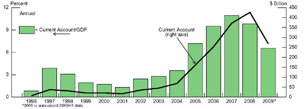
Figure 2. Chinese International Reserves

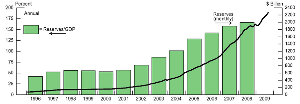
Figure 3. Chinese Exchange Rate

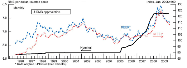
Figure 4. Change in Reserves

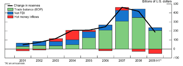
Figure 5. Processing Trade

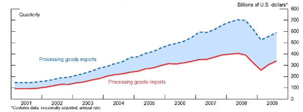
Figure 6. Non-Processing Trade

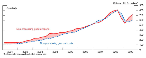
Figure 7. Comparing Exchange Rates

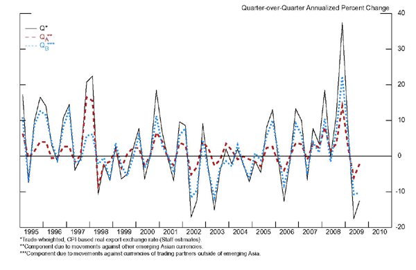
Figure 8. Actual and Fitted Export Growth: Models With Foreign Consumption and Aggregate Real Exchange Rate

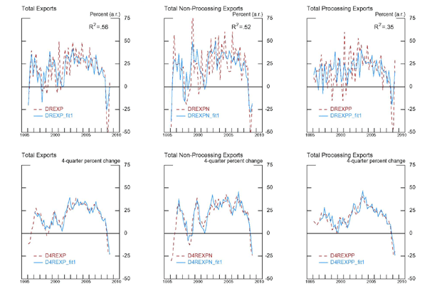
Figure 9. Actual and Fitted Export Growth: Models With Foreign Output and Aggregate Real Exchange Rate

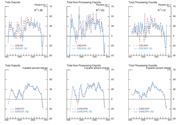
Figure 10. Actual and Fitted Export Growth: Models With Foreign Consumption and Components of Real Exchange Rate

Figure 11. Actual and Fitted Export Growth: Models With Foreign Output and Components of Real Exchange Rate

Figure 12. Counterfactual Simulation: 10 Percent Annual Real Appreciation of RMB Beginning 2005:3

Footnotes

1.  The author is Chief, Emerging Market Economies Section, Division of International Finance, Board of Governors of the Federal Reserve System, Washington, D.C. 20551, U.S.A. The views expressed in this paper are solely the responsibility of the author and should not be interpreted as reflecting the views of the Board of Governors of the Federal Reserves System or of any other person associated with the Federal Reserve System. An earlier version of this paper was presented at the 2009 Canadian Economic Association annual meetings in Toronto, Canada. I would like to thank Kavan Kucko and Nikola Kojucharov for excellent research assistance and Jeannine Baillu, Brett Berger, Carlos De Resende, Neil Ericsson, John Rogers, and Jaime Marquez, and John Schindler for very helpful comments. Return to text

2.  Ma and Sun (2007) also provide some estimates of hot money flows into China and they present a model for the behavior of these flows. Return to text

3.  To measure the exact degree of import content in exports is not a trivial matter. Dean et al (2007) do this for the case of China through measuring the vertical specialization in Chinese trade. Return to text

4.  The costs that might be incurred by the Chinese government in allowing greater flexibility of the exchange rate is also a topic of much discussion. Some papers have recently argued that the reasons most often given for why greater exchange rate adjustment would have high costs for China are flawed (see, for example, Goldstein (2007), and Goldstein and Lardy (2008)). Some authors have advocated that greater flexibility of the RMB would actually be beneficial to China's own economic interests, including allowing appropriate rebalancing of growth and pursuance of a more independent monetary polciy. Examples include Bernanke (2006), Eichengreen (2007), Lardy (2006), Prasad (2008), and a survey by Lafrance (2008).  Return to text

5.  Eamples of the studies which include the use of this approach are Anderson (2006), Cline (2007), Coudart and Couharde (2005), and Goldstein and Lardy (2008).  Return to text

6.  The other main approach to computing the extent of undervaluation is to use the PPP or the extended PPP approach. In the latter, the real exchange rate is related to a small set of variables such as per capita income ratios (the Balassa-Samuelson effect), and net foreign assset ratios and perhaps other variables. The predicted influence of these factors gives an equilibrium exchange rate which is then compared to the actual to get the misalignment. The equation could be estimated using data for a single country or based on cross-section or panel estimation. Studies pertaining to China using this approach include Cheung et al (2009), Coudert and Couharde (2005), and Frankel (2006). Cline and Williamson label only studies which incorporate the Balassa-Samuelson effect as the extended PPP approah. They prefer to label the approach with more variables being used to compute the equilibrium real effective exchange rate as the behavioural equilibrium exchange rate (BEER) approach. Return to text

7.  They compute a Chinese export price index by using a weighted average of U.S. import prices at the SITC 2-digit level, using weights that are proportional to China's share of U.S. imports in each category.  Return to text

8.  Their specification includes Chinese productivity as an indendent variable in the export equations. This makes it a bit difficult to interpret the estimated elasticity with respect to the real exchange rate, as productivity growth would normally affect the real exchange rate. However, the authors argue that, in the case of China, the Balassa-Samuelson effect "breaks down" due to the country's "large excess labor." Return to text

9.  They trace the changes over time in the price elasticity of exports to changes in the composition of trade and variation of sector-specific elasticities. They also partly attribute the changes to a rising domestic content even in processing trade.  Return to text

10.  Cheung et al use several different proxies for the Chinese export price deflator; their results are fairly robust to which proxy is used. Return to text

11.  These authors use the Chinese CPI as a proxy for Chinese export prices.  Return to text

12.  Garcia-Herrero and Koivu study also estimate import price elasticities. They find that exchange rate appreciation actually decreases rather than increases imports. Thus, real exchange rate adjustment would not help the trade balance as much as their export elasticity results suggest.  Return to text

13.  A subsequent paper, Thorbecke and Zhang (2009) focuses on disaggregated Chinese labor-intensive manufacturing exports, using the same approach. When looking at bilateral Chinese-U.S. trade, Cheung et al (2009) also included a real effective exchange rate relative to China's other trading partners, in addition to the U.S.-China bilateral real exchange rate.  Return to text

14.  Several different deflators are used as proxies fot the Chinese export price deflator. Return to text

15.  In an earlier paper, Rahman and Thorbecke (2007), $rer$ and $wrer$ were used separately in the bilateral proceesing exports equations, rather than an integrated $irer$, and different statistica techniques were also used. That resulted in estimates that were in many ways counterintuitive.  Return to text

16.  Before leaving this section reviewing previous empirical work, we should note that another completely different approach taken to determine how much Chinese trade would adjust for a given size change in the RMB is to do simulation analysis from a calibrated general-equilibrium model. We do not discuss that literature here, although an example of this approach is Wang and Whalley (2007).  Return to text

17.  Putting the imported input into the production function has also been the approach taken in a few other optimizing models of the open economy, such as McCallum and Nelson (1999) and Erceg et al (2008), although our Cobb-Douglas functional form is simpler.  Return to text

18.  In the past, this assumption has been defended by appealing to China's limitless supply of labor that can easily be moved from rural to urban areas. However, although this might be true of non-skilled workers, there is anecdotal evidence at least, of a substantial shortage of skilled or even semi-skilled workers. Therefore, the assumption of an elastic labor supply should be regarded as a simplying one, rather than a realistic one. The qualitative results derived here should not change with the introduction of an upward sloping supply curve for labor, although the exact solutions for the equilibrium quantities of labor allocated to each sector and the equilibrium quantity of the imported input would differ. Return to text

19.  In practice, China imports parts and components from outside the region as well, but most of them come from other emerging Asian countries as documented, for example, in Haltmaier et al (2009).  Return to text

20.  Some earlier studies use a series for the capital stock in manufacturing constructed in Bai et al (2006) to capture export supply effects. However, because this series does not exist for much of our sample period, it could not be used in this paper.  Return to text

21.  We have already acknowledged and disscussed Marquez and Schindler's objections to this approach.  Return to text

22.  Note that Loretan is describing the construction of U.S. exchange rate indexes, but the same approach has been followed by Federal Reserve staff in constructing the exchange rate indexes for other countries as well, including China. Return to text

23.  The one exception is $DFDIK$, where we started with a lag length of 3 to be able to start our regression estimation periods at the beginning of 1996. However, if we start the estimation one quarter later and do begin with a lag length of 4 for $DFDIK$, the fourth lag is never significant. Return to text

24.  Generally, the same model minimized all three of HQ, SC and AIC. When this was not the case, at least two of the three were minimized for the same model, which is the model that was chosen for those cases.  Return to text

25.  Equations were also estimated for aggregate exports with the two different components of the real exchange rate. The results were in between those obtained for the non-processing exports and processing exports reported here and have been excluded in the interest of brevity. Return to text

26.  In this paper, we have not studied the implications of the rise of Chinese trade for the trade of other emerging Asian economies. Such implications have been a focus of a number of papers, including Ahearne et al (2009), Eichengreen et al (2004), Haltmaier et al (2009), and Hanson (2007). Ito (2008) discusses the influence of the RMB on the exchange rate policies of the other Asian economies. Cui and Syed (2007) focus on the shifting structure of China's trade over time, including the switch to more sophisticated exports, and its implications. Return to text

27.  Note, however, that we did also conduct simulations with the foreign output growth models as well, with quite similar results. Return to text

28.  Note that the actual average annual appreciation per quarter would go down to about 4.5 percent if 2009:3 was included, given a real depreciation at an annual rate of about 12 percent in this quarter. However, our estimated equations use the sample period that ends in 2009:2.  Return to text

This version is optimized for use by screen readers. Descriptions for all mathematical expressions are provided in LaTex format. A printable pdf version is available. Return to text

Home | Economic research and data | Publications and education resources
Accessibility | Contact us
Last update: January 6, 2010