
Board of Governors of the Federal Reserve System
International Finance Discussion Papers
Number 988, December 2009 --- Screen Reader
Version*
Asset Returns with Earnings Management1
NOTE: International Finance Discussion Papers are preliminary materials circulated to stimulate discussion and critical comment. References in publications to International Finance Discussion Papers (other than an acknowledgment that the writer has had access to unpublished material) should be cleared with the author or authors. Recent IFDPs are available on the Web at http://www.federalreserve.gov/pubs/ifdp/. This paper can be downloaded without charge from the Social Science Research Network electronic library at http://www.ssrn.com/.
Abstract:
The paper investigates stock return dynamics in an environment where executives have an incentive to maximize their compensation by artificially inflating earnings. A principal-agent model with financial reporting and managerial effort is embedded in a Lucas asset-pricing model with periodic revelations of the firm's underlying profitability. The return process generated from the model is consistent with a range of financial anomalies observed in the return data: volatility clustering, asymmetric volatility, and increased idiosyncratic volatility. The calibration results further indicate that earnings management by individual firms does not only deliver the observed features in their own stocks, but can also be strong enough to generate market-wide patterns.
Keywords: Earnings management, stock returns, financial anomalies, volatility clustering, GARCH, optimal contract
JEL classification: E44, D82, D83, G12
1 Introduction
Executives' desire to use financial reports, especially bottom-line earnings, to pursue their own financial interests gives rise to the phenomenon of earnings management, which is defined as intentional manipulation of reported earnings by knowingly choosing accounting methods and estimates that do not accurately reflect the firm's underlying fundamentals. The accounting irregularities at Enron and WorldCom that precipitated the stock market downturn of 2002 and the corporate scandals that triggered the financial meltdown in 2008, notably Freddie Mac and AIG,3indicate that such behavior can engender significant economic consequences, especially in the financial markets. This paper explicitly examines the asset pricing implications of earnings management.
This intentional manipulation of financial information must be reflected in the pricing of stocks, since it affects the inference of the investors who value the stock of a firm. Empirical studies (e.g., Turner et al. [2001], Wu [2002], and Palmrose et al. [2004]) suggest that distorted information flow can cause adverse capital market reactions. In these studies, on average, stock returns fall by about 10% on the days around earnings restatement announcements. Figure 1, reproduced from Wu [2002], documents how stock returns react to restatements.4 However, due to the lack of theoretical guidance and difficulty of detecting earnings management with accuracy, comparatively little is known about the potential systematic impact of earnings management on stocks.
The objective of the present study is to analyze the implications of earnings management for dynamic patterns of asset returns. In particular, this paper shows that earnings management is a possible explanation for a number of stylized financial facts, namely, volatility clustering, asymmetric volatility, and increased idiosyncratic volatility. These results underscore why earnings management is of central importance in pricing financial assets, in understanding the risk implied by empirical financial anomalies, and in contemplating the ongoing debate on regulations of financial markets and executive compensation.
Figure 1: Cumulative Abnormal Returns Around Restatements: Day (-125, +125)
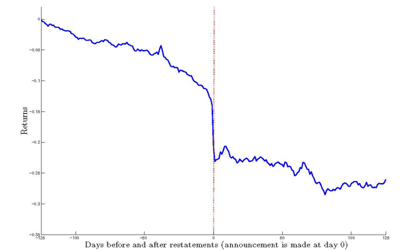
This figure displays the mean of cumulative abnormal returns of restating firms from 1977 to 2001. Day 0 is the restatement announcement date. Source: Wu [2002]
I conduct this exercise within a Lucas asset-pricing model that is standard in all aspects, except that the investors hire a manager to operate the firm and report the firm's earnings. In particular, a principal-agent model with financial reporting and productive effort is embedded in a simple variant of the Lucas asset-pricing model. The investors engage in a (single-period) contractual relationship with a newly hired manager in every period and pay the manager a fraction of the reported earnings as compensation. The manager exerts an unobserved effort that affects the production, and possibly has discretion over the quantity of apples reported to the investors. The reported earnings are paid to the investors as dividends. The key feature I focus on here is the manager's ability to manipulate earnings reports. Earnings management occurs in the model when the reported apple harvest (earnings) differs from the true amount.5
There are periodic investigations concerning the underlying true earnings of the firm. In the final period of each revelation cycle, the uncertainty about true earnings is resolved, and the investors bear monetary costs in the event that earnings management is detected.6 The investors are assumed to be risk-neutral; thus the price of the firm in each period is given by the discounted expected future dividends net of the labor wage and the financial loss associated with earnings management.
The return sequences generated from the model mimic a set of stylized facts in stock return data. First and foremost, the model returns exhibit volatility clustering. Because earnings management patterns vary with underlying true performance, certain levels of earnings lead to higher frequency of restatements than others,7 creating larger swings in the return sequence. Return volatility becomes state-dependent in the model. As the state (that is, actual earnings) exhibits persistence over time, return volatility is time-varying and persistent. In addition to the direct impact due to possible future manipulation, an indirect effect reflecting suspicion of previous misreporting amplifies the persistence in volatility. The possibility of earnings management creates a range of reports that are associated with belief revision and intense suspicion of manipulation. The anticipation of restatements increases uncertainty and hence volatility. The volatility persists as reported earnings persist. Although the conditional heteroskedasticity observed in many financial markets has led to ARCH and GARCH models that are intensively used in analyzing stock returns, the underlying microeconomic motives are still not well understood. This paper presents the persistence in earnings management behavior as a likely source of the persistence in stock return volatility.
The model data capture another stylized fact in the finance literature: asymmetric volatility in stock returns. The mechanism is also twofold. First, earnings management goes hand-in-hand with weak economic performance, due to stronger financial incentives to inflate earnings when the performance is weaker. Because current low earnings lead to more frequent future earnings manipulation and resultant drastic consequences, low returns are associated with high volatility in the subsequent periods. Second, earnings reports within certain range are viewed as symptomatic of intentional misstatement. The inference of earnings management reduces the current price and increases the uncertainty over subsequent outcomes, thereby intensifying asymmetric volatility.8 The existing literature on asymmetric volatility falls into two categories: the leverage effect proposed by Black and Scholes [1973], Merton [1974], and Black [1976] and the volatility feedback effect put forward by French et al. [1987] and Campbell and Hentschel [1992]. However, Christie [1982] and Schwert [1989] find that the leverage effect is too small to account for the asymmetry in volatility, and Campbell and Hentschel [1992] find that the volatility feedback effect normally has little impact on returns. This paper shows that the asymmetric association of earnings management to true earnings contributes to the observed asymmetric behavior in stock returns. The calibration results further suggest that this channel can be quantitatively important.
Last but not least important, as earnings management becomes more likely in the model, asset returns exhibit greater volatility. The dramatic consequences of earnings management generate active fluctuations in the return sequence and thus intensify return volatility. This work adds to a growing literature that studies individual stock return volatility. Campbell et al. [2001] document that the level of average stock return volatility increased considerably from 1962 to 1997 in the United States. Furthermore, most of this increase is attributable to idiosyncratic stock return volatility as opposed to the volatility of the stock market indices. Rajgopal and Venkatachalam [2008] explore whether deteriorating financial reporting quality, as measured by earnings quality and dispersion in analyst forecasts of future earnings, can plausibly explain the increase in idiosyncratic volatility over the past four decades. Their results from cross-sectional and time-series regressions indicate a strong association between idiosyncratic return volatility and financial reporting quality. The current model replicates the positive relationship between the likelihood of earnings management and the volatility of individual returns, and thus contributes to the theoretical explanations of the data.
In this paper, the contracting system in a principal-agent model with financial reporting and moral hazard is first examined as a point of departure. This principal-agent model is developed and analyzed in greater detail in Sun [2008]. The purpose of this step is to provide the underlying economic motive for earnings management in the model, to understand how motives to induce managerial effort and to motivate truthful reports differentially affect the optimal contract, and to identify how earnings management decisions vary with actual economic performance. This principal-agent model lays out a micro-foundation for asset pricing in that it generates a set of earnings reports that may or may not be systematically biased. This model of managerial reporting under moral hazard is built on Dye [1988]. The message space is limited to a single-dimensional signal while the privately informed agent receives two dimensions of private information; therefore the Revelation Principle is not applicable.9
In order to highlight the role that earnings management plays in price formulation, the principal-agent model with reporting choices is embedded into an otherwise standard Lucas asset-pricing model. In particular, by switching on and off the measure for earnings management in the model, I maintain the focus on earnings management and make the comparison with the standard asset-pricing model transparent. This modeling approach is related to Shorish and Spear [2005], where the owner of the firm hires a manager to maximize the firm's value, and there is asymmetric information about the manager's effort level between the owner and the manager. Along this line of agency-based asset pricing, Gorton and He [2006] show that when compensation depends on the firm's market performance, stock prices are set to induce the optimal effort level. In contrast with these papers, the current paper focuses on earnings management incentive in the contractual relationship and price formulation by assuming additional asymmetric information regarding output realizations.
This analysis also relates to the literature on asset pricing under asymmetric information, such as Detemple [1986], Wang [1993], and Cecchetti et al. [2000]. In particular, Wang [1993] presents a dynamic asset-pricing model in which the investors can be either informed or uninformed: the informed investors know the future dividend growth rate, while the uninformed investors do not. He finds that the existence of uninformed investors can lead to risk premia much higher than those under symmetric and perfect information. Distinguished from previous studies that examine the impact of information asymmetry and heterogeneous beliefs among investors, the study reported in this paper analyzes information asymmetry between corporate executives and outside investors as a whole.
There have not been many theoretical studies that examine the economic impact of earnings management. Fischer and Verrecchia [2000] is an early and notable exception. They show that more bias in the report reduces the correlation between share price and reported earnings, and they also study how the cost to the manager of biasing the report and the market's uncertainty about the manager's objective affect the slope and the intercept term in a regression of market price on earnings reports. Subsequently, Guttman et al. [2006] use a signaling model similar to Fischer and Verrecchia [2000] to explain the discontinuity observed in the distribution of earnings reports. While these papers do not model the contractual relationship between shareholders and the manager, Kwon and Yeo [2008] consider a single-period model where the principal takes into account how compensation affects productive effort and market expectations when designing the optimal contract. In their paper, a rational market can simply recalibrate or discount the reported performance when the manager overstates earnings, and correctly guess the true performance. They show that such rational market discounting leads to less productive effort by the manager and less performance pay by the principal. In contrast with the studies presented in these papers, the current study considers stock returns under earnings management in a dynamic setting, with a central focus on the return properties beyond the first moment. This study further provides a quantitative evaluation of the model.
Existing studies have analyzed earnings management behavior and stylized financial facts in isolation, and a systematic investigation into the link between earnings management and financial anomalies has not yet been undertaken. By incorporating earnings management into an otherwise standard asset-pricing model, this paper presents a mechanism through which financial misrepresentation may lead to a set of stylized financial facts. This paper suggests that there may be a unifying cause for these empirical regularities in the financial markets. In addition, the calibration results indicate that earnings management can be quantitatively important in explaining dynamic return patterns. This quantitative analysis further suggests that earnings management by individual firms may not only generate patterns in their own stock returns, but also be powerful enough to drive the observed effects in stock market indices.
The remainder of this paper proceeds as follows. Section 2 lays out the setup of the model. Section 3 discusses the general results, and presents the properties of simulated returns from the model. As one step toward calibration, Section 4 extends the model to continuous earnings. Section 5 presents a quantitative evaluation of the model. Section 6 checks the robustness of the model dynamics by adopting an alternative calibration strategy and incorporating stochastic investigation. Section 7 contains concluding remarks.
2 Model
The core of this paper is based on a Lucas asset-pricing model
in which the investors hire a manager to operate the firm and
report the firm's earnings. The investors design a contract that
controls the manager's effort decision and reporting choice. In
every period, the principal (investors) offers a newly hired
manager a single-period contract. Earnings ![]() are
stochastic and take two possible values,
are
stochastic and take two possible values,
![]() , where
, where ![]() .
The firm's production is associated with a simple Markov process:
.
The firm's production is associated with a simple Markov process:
The manager makes earnings announcements, and the reported earnings
![]() are then paid out as dividends to the
investors.10 The underlying true earnings are
periodically revealed.11 For the purpose of illustration as
well as tractability, it is assumed that after every two periods
the uncertainty about the underlying earnings in the past two
periods is resolved, and the investors bear financial losses if
earnings management is detected. The investors know the revelation
periodicity. The price of the firm in each period is given by
discounted expected future dividends net of the executive
compensation and monetary costs of earnings management.
are then paid out as dividends to the
investors.10 The underlying true earnings are
periodically revealed.11 For the purpose of illustration as
well as tractability, it is assumed that after every two periods
the uncertainty about the underlying earnings in the past two
periods is resolved, and the investors bear financial losses if
earnings management is detected. The investors know the revelation
periodicity. The price of the firm in each period is given by
discounted expected future dividends net of the executive
compensation and monetary costs of earnings management.
One interpretation of the model is that the manager finances the discrepancy in the report from a market outside the economy, and the firm's owner (the investors) must repay a large amount of money at the time earnings management is detected (this is a part of the monetary loss that the investors have to bear upon detection of manipulation). Because the current manager is replaced in the next period, the significant repayment burden imposed on the investors does not directly affect the manager's incentive.12 Another, and much broader, interpretation of the model is that the manager may engage in activities that boost current earnings at the expense of future (long-term) benefits. In particular, the manager may follow myopic strategies and take economically suboptimal actions to inflate current earnings, such as forsaking profitable investment and postponing R&D and capital spending plans.13 This interpretation corresponds to a more general notion of earnings management this model captures, which is an overstatement of current earnings that has negative consequences for the firm's future prospects.14
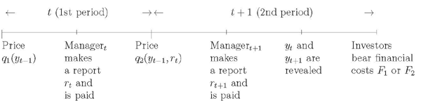
Figure 2: Timeline of Contracting Within Each Period
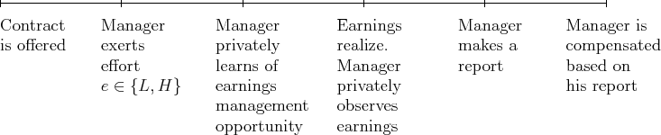
2.1 Optimal Contract
The contractual environment follows Sun [2008]. A risk-neutral principal (investors) hires a risk-averse agent (manager) for one period. Figure 2 details the timeline of the contracting arrangement between the principal and the manager. In the beginning of each period,
the manager accepts the take-it-or-leave-it contract offered by
the principal for one period. Earnings are stochastic and
influenced by the manager's effort. The unobserved effort level of
the manager, ![]() , can take two values, low
, can take two values, low ![]() and high
and high ![]() . The manager incurs
disutility from exerting effort, denoted by the cost function
. The manager incurs
disutility from exerting effort, denoted by the cost function
![]() . In particular, high effort is
associated with a cost of
. In particular, high effort is
associated with a cost of ![]() , and low
effort involves no cost:
, and low
effort involves no cost: ![]() . Earnings take two
possible values, represented by
. Earnings take two
possible values, represented by
![]() , where
, where ![]() .
Let
.
Let ![]() be the probability that earnings are
be the probability that earnings are
![]() when the effort is
when the effort is ![]() , with
, with
![]() . After exerting effort, the
manager privately learns whether he has the opportunity to manage
earnings. With probability
. After exerting effort, the
manager privately learns whether he has the opportunity to manage
earnings. With probability ![]() , the manager has
discretion over how much earnings to report.15 With probability
, the manager has
discretion over how much earnings to report.15 With probability
![]() , the manager is prohibited from
manipulating earnings. Then the manager privately observes the
earnings, and makes an earnings announcement.
, the manager is prohibited from
manipulating earnings. Then the manager privately observes the
earnings, and makes an earnings announcement.
If the manager produces an inaccurate report, the manager incurs
a personal cost, denoted by
![]() .
. ![]() is a
function of the discrepancy between true earnings and reported
earnings. When the manager reports honestly, he incurs no cost:
is a
function of the discrepancy between true earnings and reported
earnings. When the manager reports honestly, he incurs no cost:
![]() .16 When the manager
overstates earnings, there is a positive cost
.16 When the manager
overstates earnings, there is a positive cost
![]() . Earnings management
occurs in the model when the reported earnings differ from true
earnings. More specifically, earnings management emerges in this
environment if the manager announces that high earnings
. Earnings management
occurs in the model when the reported earnings differ from true
earnings. More specifically, earnings management emerges in this
environment if the manager announces that high earnings ![]() have been achieved when the actual realization of
earnings is low
have been achieved when the actual realization of
earnings is low ![]() .
.
As the contract must be designed based on mutually observed
variables, the manager's compensation can be based only on the
earnings report. As long as the manager's reported earnings fall in
the set ![]() , the principal cannot directly
detect whether the manager has misstated earnings. For notation
convenience, high and low reported earnings are denoted by
, the principal cannot directly
detect whether the manager has misstated earnings. For notation
convenience, high and low reported earnings are denoted by
![]() and by
and by ![]() , to
distinguish from high and low actual earnings.17 It is also
assumed that the manager is essential to the operation of the firm,
so the contract must be such that the manager (weakly) prefers to
work for the principal regardless of whether the manager gains the
opportunity to manage earnings.
, to
distinguish from high and low actual earnings.17 It is also
assumed that the manager is essential to the operation of the firm,
so the contract must be such that the manager (weakly) prefers to
work for the principal regardless of whether the manager gains the
opportunity to manage earnings.
The contract between the risk-neutral principal and the
risk-averse agent includes a set of wages contingent on the
reports, which can be alternatively characterized as a set of
contingent utilities. The manager's utility level corresponding to
compensation level ![]() ,
,
![]() , is denoted as
, is denoted as
![]() , where
, where ![]() is a strictly increasing and strictly concave
utility function. Let
is a strictly increasing and strictly concave
utility function. Let
![]() . Then
. Then ![]() is the cost to the principal of providing the agent
with utility
is the cost to the principal of providing the agent
with utility ![]() . Because
. Because ![]() is a strictly increasing and strictly concave function,
is a strictly increasing and strictly concave function, ![]() is a strictly increasing and strictly convex
function.
is a strictly increasing and strictly convex
function.
In this environment, the contract must not only induce effort
but also control for the manager's reporting incentive. This study
assumes that the difference in the earnings is large enough that
the principal always wants to implement high effort. The objective
of the manager is to maximize utility by choosing a level of effort
and a reporting strategy represented by ![]() , subject
to the contract offered. When the manager has no discretion, we
denote the report by
, subject
to the contract offered. When the manager has no discretion, we
denote the report by ![]() . By assumption,
. By assumption,
![]() .
The manager's utility is of the form
.
The manager's utility is of the form
![]() . The first term is the manager's expected utility if the manager
has sufficient discretion over reporting. The second term is the
manager's expected utility if the manager has to truthfully report.
The principal chooses the utility values
. The first term is the manager's expected utility if the manager
has sufficient discretion over reporting. The second term is the
manager's expected utility if the manager has to truthfully report.
The principal chooses the utility values ![]() ,
,
![]() , and recommended
reporting choices
, and recommended
reporting choices ![]() for each realization of
earnings that minimize the expected cost of inducing
effort.18
for each realization of
earnings that minimize the expected cost of inducing
effort.18
Formally, the optimal contract solves
![\begin{displaymath} \begin{array}[c]{rl} \displaystyle\mathop{\min}_{u_{\tilde h}, u_{\tilde l}, R(h), R(l)} & \ E [ V (u) \vert H]\ & = x [ p_{H} V(u_{R(h)})+(1-p_{H}) V(u_{R(l)})] + (1-x) [p_{H} V(u_{\tilde h})+(1-p_{H})V(u_{\tilde l})] \end{array}\end{displaymath}](img70.gif)
subject to
![$\displaystyle H = \mathop{\arg \max}_{e \in\{L,H \}} x E[ u_{R(y)}-\phi(R(y)-y)-a(e)]+(1-x) E [ u_{\bar R(y)}-a(e) ], \quad\quad\forall y \in\{ l,h \}.$](img71.gif) |
(1) |
| (2) |
The objective function is the expected cost for the principal to
motivate high effort. The first term is the cost of implementing
high effort when the manager has an opportunity to manage earnings,
and the second term is the cost if the manager does not have the
opportunity. The first constraint is the incentive constraint for
the manager's effort choice -- here, it is assumed that the
principal wants to induce high effort. The second is the
participation constraint, where ![]() is the
manager's outside option. In addition to these constraints, when
the manager has an opportunity to misstate earnings, the principal
faces another constraint. As the reporting decision has been
necessarily delegated to the manager, the "recommended reporting
strategy" has to be voluntarily followed by the manager:
is the
manager's outside option. In addition to these constraints, when
the manager has an opportunity to misstate earnings, the principal
faces another constraint. As the reporting decision has been
necessarily delegated to the manager, the "recommended reporting
strategy" has to be voluntarily followed by the manager:
 |
(3) |
The optimal contract includes a set of utility promises
![]() and the
recommended action
and the
recommended action
![]() . Following the convention, it
is assumed that the principal wants to induce high effort, so
. Following the convention, it
is assumed that the principal wants to induce high effort, so
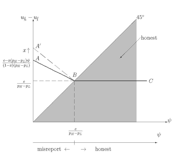
![]() . Figure 3 summarizes the main results. The optimal
contract is described as the curve
. Figure 3 summarizes the main results. The optimal
contract is described as the curve ![]() , which
depicts how the wedge between promised utilities assigned to
reports of high and low earnings varies with different values of
manipulation cost
, which
depicts how the wedge between promised utilities assigned to
reports of high and low earnings varies with different values of
manipulation cost ![]() . The shaded area below
the
. The shaded area below
the
![]() line shows the combination of the
compensation differential and manipulation cost that induces
truthful reporting. Below I restate the relevant results shown in
Sun [2008].
line shows the combination of the
compensation differential and manipulation cost that induces
truthful reporting. Below I restate the relevant results shown in
Sun [2008].
Proposition 1
![]() is the necessary and
sufficient condition for earnings management to occur under the
optimal contract.
is the necessary and
sufficient condition for earnings management to occur under the
optimal contract.
Figure 3: Main Results
Lemma 1 If
![]() holds, the optimal
contract satisfies
holds, the optimal
contract satisfies
 |
(4) |
 |
(5) |
The contract model illustrates the necessary and sufficient condition for earnings management to occur, and it yields a number of empirical implications of how earnings management affects executive compensation that are in line with empirical findings, which are detailed in Sun [2009]. In the current paper, this principal-agent model derives the manager's motive to manage earnings and also serves as a micro-foundation for asset pricing. Given a sequence of true earnings, the contract model generates a set of reports that may or may not be systematically biased. Because the realization of manipulation opportunity is stochastic, the investors are not able to make perfect inferences as to whether a report has been manipulated. As a micro-foundation for asset pricing, the central features this contract model boils down to are (1) the investors' inability to see through earnings management and (2) a focus on the upward manipulation of earnings.19 The analysis below assumes that the condition for earnings management to occur is met so that the manager always overstates earnings when the earnings are low and the earnings management opportunity arises.
Figure 4: Model Timeline
In this figure q1 and q2 are the pricing functions in period 1 and 2 of each revelation cycle respectively. yt-1 is the actual earnings in period 2 of the previous revelation cycle. yt and yt+1 are actual earnings in period 1 and period 2 in the current revelation cycle. F1 and F2 are the amount of financial loss investors bear if the manager manipulates earnings in one period and that if the manager manipulates earnings in both periods in the current revelation cycle.
2.2 Asset Prices
Now, this contract model is embedded into a dynamic model of
asset pricing. It is assumed that the earnings process is
persistent: the true earnings at time ![]() ,
, ![]() , depend on
, depend on ![]() in addition to the
manager's current effort. In particular, under the high effort by
the manager (which is always the case in the equilibrium I
consider), I assume that the true earnings follow a Markov process
with transition probability
in addition to the
manager's current effort. In particular, under the high effort by
the manager (which is always the case in the equilibrium I
consider), I assume that the true earnings follow a Markov process
with transition probability
![]() , where
, where ![]() is the earnings at time
is the earnings at time ![]() and
and
![]() is the earnings at time
is the earnings at time
![]() . The asset price is determined as the
present value of dividends, which are reported earnings net of the
compensation and financial losses associated with earnings
management. Figure
. The asset price is determined as the
present value of dividends, which are reported earnings net of the
compensation and financial losses associated with earnings
management. Figure
![]() chronicles the timeline of the model. It describes the timing of
the events in two consecutive periods
chronicles the timeline of the model. It describes the timing of
the events in two consecutive periods ![]() and
and
![]() , and this two-period revelation cycle
repeats over time. Because the model is stationary, all the
relevant past information is summarized in the previously revealed
earnings and current reported earnings.
, and this two-period revelation cycle
repeats over time. Because the model is stationary, all the
relevant past information is summarized in the previously revealed
earnings and current reported earnings.
In the first period of the two-period revelation cycle
(hereafter, period 1), the price of the firm
![]() is determined based on the
revelation of the previous period's earnings
is determined based on the
revelation of the previous period's earnings ![]() . Having the manager's reporting incentive in mind,
the investors form their expectations about future dividend income
based on the revelation of the firm's previous earnings
. Having the manager's reporting incentive in mind,
the investors form their expectations about future dividend income
based on the revelation of the firm's previous earnings ![]() . In the second period of each cycle (hereafter,
period 2), given the earnings report in the first period
. In the second period of each cycle (hereafter,
period 2), given the earnings report in the first period
![]() and the true outcome in the ending
period of the last cycle
and the true outcome in the ending
period of the last cycle ![]() , the firm is priced
as
, the firm is priced
as
![]() . After the manager
reports the earnings and pays them out entirely to the investors,
the investigation takes place. When the investigation is conducted,
the true realization of earnings in each period of the cycle is
revealed, and the investors bear financial costs associated with
any misstatement of earnings that occurs during the cycle. If the
report is inflated in one of the two periods, the investors incur
an amount of financial losses
. After the manager
reports the earnings and pays them out entirely to the investors,
the investigation takes place. When the investigation is conducted,
the true realization of earnings in each period of the cycle is
revealed, and the investors bear financial costs associated with
any misstatement of earnings that occurs during the cycle. If the
report is inflated in one of the two periods, the investors incur
an amount of financial losses ![]() . If earnings
management occurs in both periods, the investors must pay an amount
of monetary costs
. If earnings
management occurs in both periods, the investors must pay an amount
of monetary costs ![]() , where
, where
![]() .
.
I assume that the investors have linear utility and maximize the
sum of the expected dividends. Then the value of the firm can be
formulated as follows. In the beginning of an revelation cycle,
given the revelation of the true outcome in the end of the last
cycle ![]() , the price of the firm
, the price of the firm
![]() is given by the expected sum
of the net dividends and asset price in the next period (the time
subscript is dropped when the timing is clear):
is given by the expected sum
of the net dividends and asset price in the next period (the time
subscript is dropped when the timing is clear):
|
(6) |
and
|
(7) |
where ![]() is the net dividend income and
is the net dividend income and
![]() is the investors' discount factor. The
net dividend income equals the reported earnings less the
compensation, that is,
is the investors' discount factor. The
net dividend income equals the reported earnings less the
compensation, that is,
![]() , where
, where
![]() .
.
Regardless of the revelation of ![]() in
period
in
period ![]() , the investors may encounter three
possible states in period
, the investors may encounter three
possible states in period ![]() . The first term in (6) and (7) is the expected net
dividend income if the manager sends an honest report of high
earnings in the next period. The second term in (6) and (7) represents the case in which
the actual realization of earnings is low, but the manager makes an
overstatement of earnings. The third term in the prices is the case
in which the manager truthfully reports low earnings.
. The first term in (6) and (7) is the expected net
dividend income if the manager sends an honest report of high
earnings in the next period. The second term in (6) and (7) represents the case in which
the actual realization of earnings is low, but the manager makes an
overstatement of earnings. The third term in the prices is the case
in which the manager truthfully reports low earnings.
Given the first-period report ![]() and the
previously revealed outcome
and the
previously revealed outcome ![]() , the
investors update their belief about the true state in period 1. If
the first-period report is low, it is for certain an honest report.
If the report sent by the manager is high, it may be an overstated
report that leads to immediate penalties. The posterior belief of
the first-period report being truthful is derived following Bayes'
Rule. If the previously revealed outcome is high, the conditional
probability of
, the
investors update their belief about the true state in period 1. If
the first-period report is low, it is for certain an honest report.
If the report sent by the manager is high, it may be an overstated
report that leads to immediate penalties. The posterior belief of
the first-period report being truthful is derived following Bayes'
Rule. If the previously revealed outcome is high, the conditional
probability of ![]() , denoted by
, denoted by
![]() , is
, is
 |
||
 |
||
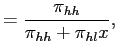 |
If the previously revealed outcome is low, the conditional
probability of ![]() , denoted by
, denoted by
![]() , is
, is
 |
||
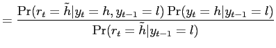 |
||
 |
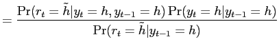
The price of the firm
![]() is determined using
these posterior probabilities. There are two cases. First, if
period 1's report is low, the investors know that the realization
of earnings is low.
is determined using
these posterior probabilities. There are two cases. First, if
period 1's report is low, the investors know that the realization
of earnings is low.
| (8) |
Because actual earnings follow a Markov process, the most recent realization of earnings is the only useful information for predicting future earnings. The price in response to a low report (which implies a realization of low earnings) is thus independent of the previous revelation of earnings, equal to the expected payoff over three possible states in the next period. The first term in (8) is the expected net dividend income if the manager sends an honest report of high earnings in the current period. The second term in (8) represents the case in which the manager makes an overstatement of earnings that leads to immediate financial losses. The third term in prices is associated with the situation in which the manager truthfully reports low earnings.
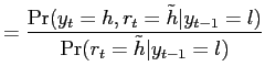
If the report just sent by the manager in period 1 is high, the report may or may not be truthful. Prices are determined as follows:
|
(9) |
|
(10) |
The first term in (9) and (10) corresponds to the case where the first-period
report is honest. In this case, there are three possible situations
in the next period. In particular, if the realization of the
second-period earnings is low and the manager has an opportunity to
inflate earnings, the manager will report high. An amount of
monetary penalties ![]() will be charged and
thus subtracted in the pricing equation. The second term in (9) and (10) represents the
case in which the first-period report is false. There are again
three possible states in the second period. The investors suffer
from an amount of financial losses
will be charged and
thus subtracted in the pricing equation. The second term in (9) and (10) represents the
case in which the first-period report is false. There are again
three possible states in the second period. The investors suffer
from an amount of financial losses ![]() if the
manager truthfully presents earnings in period 2 and an amount
if the
manager truthfully presents earnings in period 2 and an amount
![]() if the manager manipulates earnings in
period 2.
if the manager manipulates earnings in
period 2.
The manager's overstatement of earnings enables the investors to
enjoy a higher level of current period consumption than they would
in the absence of earnings management; however, this practice also
exposes the investors to the loss from earnings restatement risk,
that is, the subsequent financial cost after the periodic
investigations. The net dividends in period ![]() equal
the reported earnings net of the compensation, that is,
equal
the reported earnings net of the compensation, that is,
![]() , where
, where
![]() .20 If
.20 If
![]() ,
the cost of financial misreporting overwhelms the benefit.
Everything else constant, all the prices decrease as
,
the cost of financial misreporting overwhelms the benefit.
Everything else constant, all the prices decrease as ![]() rises. I restrict my attention to this case throughout this
analysis.21
rises. I restrict my attention to this case throughout this
analysis.21
2.3 Comparative Statics
The price differential between ![]() and
and
![]() measures how sensitive the firm's
price
measures how sensitive the firm's
price
![]() is in response to the
investigation results
is in response to the
investigation results ![]() . How does
. How does
![]() change as the opportunity
of earnings management,
change as the opportunity
of earnings management, ![]() , changes? To examine this,
let us first ignore that the wage of the manager actually changes
with
, changes? To examine this,
let us first ignore that the wage of the manager actually changes
with ![]() . It can be shown that as long as the
firm's stochastic production process is persistent, that is,
. It can be shown that as long as the
firm's stochastic production process is persistent, that is,
![]() , the price becomes
more responsive to investigation results as
, the price becomes
more responsive to investigation results as ![]() increases. Under the condition that
increases. Under the condition that
![]() ,
both
,
both ![]() and
and ![]() fall
as
fall
as ![]() escalates. However,
escalates. However, ![]() diminishes faster than
diminishes faster than ![]() ,
because a low previous output implies that future outputs tend to
be low as well, imposing greater exposure to earnings restatement
risk.
,
because a low previous output implies that future outputs tend to
be low as well, imposing greater exposure to earnings restatement
risk.
The analysis above does not consider that wages and thus net
dividend income change with ![]() . However, the same
qualitative result holds even if the change in the compensation is
taken into account. The optimal contract in this environment is
characterized by (4) and (5).
It can be seen that the compensation for the report of high
earnings is independent of
. However, the same
qualitative result holds even if the change in the compensation is
taken into account. The optimal contract in this environment is
characterized by (4) and (5).
It can be seen that the compensation for the report of high
earnings is independent of ![]() , and the
compensation for low earnings reports decreases as
, and the
compensation for low earnings reports decreases as ![]() expands. Therefore, as
expands. Therefore, as ![]() becomes greater, the net
dividend income from a report of high earnings, that is,
becomes greater, the net
dividend income from a report of high earnings, that is,
![]() , remains
the same, whereas the net dividend from a low earnings report,
, remains
the same, whereas the net dividend from a low earnings report,
![]() ,
increases, resulting in a smaller dividend differential between
high and low reports. Assuming that the monetary costs
,
increases, resulting in a smaller dividend differential between
high and low reports. Assuming that the monetary costs ![]() and
and ![]() do not vary with
do not vary with ![]() , as the financial gain from earnings management,
represented by
, as the financial gain from earnings management,
represented by
![]() , diminishes,
earnings management becomes more financially costly to the
investors. The prices thus drop more as
, diminishes,
earnings management becomes more financially costly to the
investors. The prices thus drop more as ![]() rises. The
change in the compensation schedule in response to the change of
rises. The
change in the compensation schedule in response to the change of
![]() internalizes the financial gain from
earnings management, and it reinforces the amplification of the
price differential and hence the price volatility.
internalizes the financial gain from
earnings management, and it reinforces the amplification of the
price differential and hence the price volatility.
Keeping the revelation of previous earnings constant, the price
wedge in response to different reports in the ending period of one
cycle, as measured by
![]() , does
not necessarily have a monotonic relationship with
, does
not necessarily have a monotonic relationship with ![]() .
To see this in a relatively straightforward manner, let us first
ignore the effect of
.
To see this in a relatively straightforward manner, let us first
ignore the effect of ![]() on the manager's wages.
on the manager's wages.
![]() is decreasing in
is decreasing in
![]() because of two forces that reinforce each
other. First, as
because of two forces that reinforce each
other. First, as ![]() rises, it is more likely to have
false reports in future. These falsified reports lead to the
investors' financial losses. Second, it is also more likely that
the previous report
rises, it is more likely to have
false reports in future. These falsified reports lead to the
investors' financial losses. Second, it is also more likely that
the previous report ![]() is a false report,
resulting in penalties waiting to be paid. Because
is a false report,
resulting in penalties waiting to be paid. Because ![]() in
in
![]() is surely an honest
report, the second force is absent. However, we do not necessarily
obtain a smaller gap between
is surely an honest
report, the second force is absent. However, we do not necessarily
obtain a smaller gap between
![]() and
and
![]() as
as ![]() increases. Because of the high persistence in the earnings process,
the first force works stronger for
increases. Because of the high persistence in the earnings process,
the first force works stronger for
![]() than for
than for
![]() . The impact of changes in
. The impact of changes in
![]() on the price volatility remains ambiguous
in this case.
on the price volatility remains ambiguous
in this case.
There are additional effects to consider if we take into account
the impact of ![]() on compensation schedule. Recall that
the compensation structure in this environment exhibits the
property that as earnings management becomes more likely, the
compensation wedge is magnified, leading to a smaller dividend
differential. As earnings management becomes more costly to the
investors, prices decline more when
on compensation schedule. Recall that
the compensation structure in this environment exhibits the
property that as earnings management becomes more likely, the
compensation wedge is magnified, leading to a smaller dividend
differential. As earnings management becomes more costly to the
investors, prices decline more when ![]() increases.
This response of the wage payment to changes in
increases.
This response of the wage payment to changes in ![]() strengthens the first mechanism that is at work for both
strengthens the first mechanism that is at work for both
![]() and
and
![]() without affecting the
other mechanism that works only for
without affecting the
other mechanism that works only for
![]() . Although the net effect
of
. Although the net effect
of ![]() on the price volatility could spin either
way in the second period of one cycle, incorporating the change in
the compensation scheme generates higher price volatility than
otherwise.
on the price volatility could spin either
way in the second period of one cycle, incorporating the change in
the compensation scheme generates higher price volatility than
otherwise.
From this point forward in this paper, I will ignore the wage values in the price calculation, so as not to complicate the mechanism and conflate with the main argument. The channel that earnings management influences returns through wages should be quantitatively weak, because executive compensation, although sizable and growing, does not constitute a substantial fraction of firms' earnings.22
The asset return is calculated as the sum of the current period price and dividends divided by the previous period price and then subtracted by one. The return volatility in the model is measured as the average return volatility in each period. When earnings management becomes likely, restatement risk amplifies the movement of returns and thus raises return volatility. Analogously, in order to compare the conditional volatility difference in response to earnings revelations, I use the difference between the average return volatility following a revelation of high earnings and that following a revelation of low earnings. Earnings management risk increases the volatility difference, because low earnings generate financial incentives for the manager to overstate earnings while high earnings do not. In particular, a previous low output equalizes the distribution of current reports and hence raises uncertainty in period 1, and it also leads to a greater likelihood and amount of financial loss in period 2, magnifying the return volatility in both periods. Now that return volatility depends on the true state of the firm, given a persistent state evolution process, the volatility is also persistent.
Table 1. Parameter Values in the Numerical Example with Binary Earnings
| Parameter | Description | Value |
|---|---|---|
| Level of high earnings | ||
| Level of low earnings | 0 | |
| Transition probability: | ||
| Transition probability: | ||
| Discount factor | ||
| Monetary loss for one restatement | | |
| Monetary loss for two restatements |
3 Results
In this section, I solve the model numerically and present the results from model simulations. Table 1 shows the parameter values in the numerical example.23The primary purpose in this section is to illustrate that earnings management can generate a number of stylized financial facts. The quantitative results will be presented in Section 5.24
3.1 Volatility Clustering and Asymmetric Volatility
For the illustrative purpose, I use ![]() and
and
![]() as an example to demonstrate the
impact of earnings management throughout this section. The
simulated return sequence from the model captures the stylized
facts of conditional volatility: first, conditional volatility
exhibits persistence; second, stock returns are negatively
correlated with the volatility of subsequent returns.
as an example to demonstrate the
impact of earnings management throughout this section. The
simulated return sequence from the model captures the stylized
facts of conditional volatility: first, conditional volatility
exhibits persistence; second, stock returns are negatively
correlated with the volatility of subsequent returns.
The EGARCH (1,1) model of the return series is estimated using
Maximum Likelihood method with 10,000 artificially generated
observations. The EGARCH (1,1) model used is
![]() , where
, where ![]() is the expectation operator,
is the expectation operator,
![]() is the innovation, and
is the innovation, and
![]() is the conditional variance of
the innovation. The
is the conditional variance of
the innovation. The ![]() term captures volatility
clustering (that is, persistence of volatility). A positive value
of the
term captures volatility
clustering (that is, persistence of volatility). A positive value
of the ![]() term in the equation implies that a
deviation of the standardized innovation from its expected value
causes the variance to be larger than otherwise. The
term in the equation implies that a
deviation of the standardized innovation from its expected value
causes the variance to be larger than otherwise. The ![]() coefficient allows this effect to be asymmetric.25
coefficient allows this effect to be asymmetric.25
Table 2 presents the results. The upper
panel presents the case without earnings management, that is,
![]() . In this case, there is no GARCH or ARCH
effect present in the simulated return data. As
. In this case, there is no GARCH or ARCH
effect present in the simulated return data. As ![]() becomes positive, return volatility becomes serially correlated.
Before estimation, the Lagrange Multiplier (LM) test is applied to
the return data, and the LM test strongly rejects the i.i.d.
residual hypothesis at the 95% confidence
level. The coefficients of the EGARCH (1,1) model are all
statistically significant beyond the 95% confidence level. In addition, the conditional variance process is
strongly persistent (with
becomes positive, return volatility becomes serially correlated.
Before estimation, the Lagrange Multiplier (LM) test is applied to
the return data, and the LM test strongly rejects the i.i.d.
residual hypothesis at the 95% confidence
level. The coefficients of the EGARCH (1,1) model are all
statistically significant beyond the 95% confidence level. In addition, the conditional variance process is
strongly persistent (with ![]() coefficient =
0.60). The negative value of the coefficient L shows evidence of
asymmetry in the model return behavior -- negative surprises
increase volatility more than positive surprises.
coefficient =
0.60). The negative value of the coefficient L shows evidence of
asymmetry in the model return behavior -- negative surprises
increase volatility more than positive surprises.
Table 2a. EGARCH (1,1) Estimation Results (Binary Earnings) -![]() =0
=0
| Coefficient | Std.Error | T-statistic | |
|---|---|---|---|
| -5.0000 | 0.4153 | -12.0387 | |
| -0.0001 | 0.6829 | 0.0001 | |
| 0.0000 | 0.0087 | 0.0000 | |
| 0.0009 | 0.0092 | 0.1049 |
Table 2b. EGARCH (1,1) Estimation Results (Binary Earnings) -![]() =0.1
=0.1
| Coefficient | Std.Error | T-statistic | |
|---|---|---|---|
| -1.8621 | 0.3136 | -5.9380 | |
| 0.5999 | 0.0663 | 9.0545 | |
| 0.0407 | 0.0058 | 6.9856 | |
| -0.1125 | 0.0278 | -4.0553 |
This table reports the estimates of
the EGARCH coefficients in the binary example. Maximum likelihood
is used to estimate the coefficients needed to fit the following
EGARCH model to the model return series:
![]() , where
, where
![]() is an innovation and
is an innovation and
![]() is the conditional variance of
the innovation. The model return is simulated for 10,000 periods.
is the conditional variance of
the innovation. The model return is simulated for 10,000 periods.
![]() is the probability that the manager is
able to manipulate earnings in one period.
is the probability that the manager is
able to manipulate earnings in one period.
The persistence and asymmetry in the conditional volatility of stock returns in the model are generated by earnings management incentive together with a persistent earnings process. When true earnings are revealed to be low, the persistence in the earnings-generating process implies that earnings tend to stay low for a while, so earnings management is likely to occur in the current and future periods. A higher frequency of occurrence of earnings management increases future return volatility. If the previous earnings are revealed to be high, the current and future earnings are likely to remain high. Overstatement of earnings has little chance of occurring; thereby future returns are relatively stable in this case. As a result, the volatility of the return series is persistent, and returns are negatively correlated with the subsequent volatility.26
3.2 Return Volatility
Table 3. Volatility of the Model Returns (Binary Earnings)
| Standard Deviation | |
|---|---|
| 0 | 0.0954 |
| 0.1 | 0.1015 |
| 0.2 | 0.1086 |
This table reports the standard
deviation of returns in the numerical example with binary earnings.
![]() is the probability that the manager is
able to manipulate earnings in one period.
is the probability that the manager is
able to manipulate earnings in one period.
Table 3 presents the volatility of the simulated returns. Monetary losses
that incur during revelations generate large swings in the return
sequence and hence produce volatility. When earnings management and
earnings restatements occur more frequently, returns become more
volatile. Campbell et al. [2001] document that idiosyncratic stock
return volatility increased considerably from 1962 to 1997 in the
United States. Rajgopal and Venkatachalam [2008] report a strong
association between idiosyncratic return volatility and financial
reporting quality, as measured by both earnings quality and
forecast dispersion, in both cross-sectional and time-series
regressions. In line with the empirical findings, as ![]() increases in the model, implying that the informativeness
of earnings reports becomes weakened, the returns exhibit greater
volatility.
increases in the model, implying that the informativeness
of earnings reports becomes weakened, the returns exhibit greater
volatility.
4 Extension to Continuous Earnings
In this section,the model is extended to the case with a
continuum of earnings. This model is used for the quantitative
analysis in the next section. In the continuous case, I assume that
earnings follow an AR(1) process:
![]() , where
, where
![]() ,
, ![]() is a
constant, and
is a
constant, and ![]() is a white noise process with
zero mean and standard deviation
is a white noise process with
zero mean and standard deviation ![]() .
.
4.1 Optimal Contract
Analogous to the binary model elaborated above, a risk-neutral
principal (investors) hires a risk-averse agent (manager) for one
period. Expending high effort incurs a utility cost, that is,
![]() , to the manager, whereas low effort
involves no cost. The manager's effort decision and an exogenous
state realization together determine the firm's economic earnings,
which are privately observed by the manager. The conditional
distributions of earnings given high and low effort follow normal
distributions:
, to the manager, whereas low effort
involves no cost. The manager's effort decision and an exogenous
state realization together determine the firm's economic earnings,
which are privately observed by the manager. The conditional
distributions of earnings given high and low effort follow normal
distributions:
![]() and
and
![]() ,
where
,
where
![]() . After exerting effort,
the manager privately learns whether an opportunity is available to
inflate earnings in the manager's favor. With probability
. After exerting effort,
the manager privately learns whether an opportunity is available to
inflate earnings in the manager's favor. With probability
![]() , the manager has discretion to overstate
earnings by a constant amount
, the manager has discretion to overstate
earnings by a constant amount ![]() , and a utility
cost
, and a utility
cost
![]() is involved in such earnings
manipulation. In particular,
is involved in such earnings
manipulation. In particular,
![]() . With probability
. With probability
![]() , the applicable accounting rules are
so hard-and-fast that the manager has no option but truthfully
present earnings. The manager's outside option is
, the applicable accounting rules are
so hard-and-fast that the manager has no option but truthfully
present earnings. The manager's outside option is ![]() .
.
The model is extended to the case with continuous earnings by
characterizing the optimal wage function contingent on the earnings
reports. The optimal wage schedule is numerically computed in Sun
[2008], utilizing Simulated Annealing algorithm with Gauss Hermite
quadrature. In the numerical implementation, it is always the case
that under the optimal contract, there exists a threshold level of
earnings ![]() , above which the manager does not find
it worthwhile to manipulate earnings and truth-telling strategy is
thus maintained. Below this threshold, the manager achieves
personal gains from manipulation and inflates earnings whenever
possible. Thereafter, this paper focuses on this threshold-style of
reporting behavior.
, above which the manager does not find
it worthwhile to manipulate earnings and truth-telling strategy is
thus maintained. Below this threshold, the manager achieves
personal gains from manipulation and inflates earnings whenever
possible. Thereafter, this paper focuses on this threshold-style of
reporting behavior.
The intuition behind the existence of the threshold earnings that separates truthful reporting and earnings management is as follows. Given that the manager is risk averse, a wage function that is not too convex translates into a set of concave utility promises. As actual earnings expand, the manager faces a decreasing utility gain but a constant utility cost from overstating earnings. As a consequence, earnings management occurs when the realized earnings are relatively low, and a truthful reporting strategy is sustained if actual earnings are high.
4.2 Asset Prices
The pricing formulation is extended to the continuous case as follows.27Based on the revelation of previous earnings, the price in period 1 is determined as the expected sum of the dividends and price in the next period:
|
(13) |
The first term in the pricing function represents the case when the
actual earnings in the next period exceed the threshold level of
earnings that elicits the truth, and therefore the manager reports
honestly. The second term in (13) is the case
when the next period's actual earnings fall below the threshold
earnings, and the manager has an opportunity to manage earnings.
The manager in this case overstates earnings. In particular, the
next period's report is
![]() . The third term
in (13) represents the situation in which the
next period's earnings are below the threshold earnings, but the
manager does not have the earnings management opportunity. In this
case, the manager has to truthfully represent the earnings.
. The third term
in (13) represents the situation in which the
next period's earnings are below the threshold earnings, but the
manager does not have the earnings management opportunity. In this
case, the manager has to truthfully represent the earnings.
The price in period 2 is a function of the previously revealed earnings and the earnings report in period 1.
where
and
Here, ![]() is the expected present value of the
dividends when the first-period report is truthful, and
is the expected present value of the
dividends when the first-period report is truthful, and
![]() corresponds to the case where
the first-period report is false. Similar to the pricing function
in period 1, the first term in
corresponds to the case where
the first-period report is false. Similar to the pricing function
in period 1, the first term in ![]() and
and
![]() represents the case when the
second-period earnings are higher than the threshold earnings, and
the reported earnings are truthful. In
represents the case when the
second-period earnings are higher than the threshold earnings, and
the reported earnings are truthful. In
![]() ,
, ![]() is
subtracted because investors must bear monetary penalties for the
earnings management practice in period 1 of this revelation cycle.
The second term in
is
subtracted because investors must bear monetary penalties for the
earnings management practice in period 1 of this revelation cycle.
The second term in ![]() and
and
![]() represents the case when the
actual earnings in period 2 are lower than the threshold earnings,
and the manager has discretion to inflate earnings by
represents the case when the
actual earnings in period 2 are lower than the threshold earnings,
and the manager has discretion to inflate earnings by ![]() . In this case, the investors pay
. In this case, the investors pay ![]() for
the overstatement if the first-period report is honest (as in
for
the overstatement if the first-period report is honest (as in
![]() ) and
) and ![]() if the
first-period report is also falsified (as in
if the
first-period report is also falsified (as in
![]() ). The third term is the case
when the manager does not have sufficient discretion over reporting
in period 2 and has to truthfully report the earnings that fall
below the threshold earnings. In
). The third term is the case
when the manager does not have sufficient discretion over reporting
in period 2 and has to truthfully report the earnings that fall
below the threshold earnings. In
![]() , the deduction of
, the deduction of ![]() is due to the earnings overstatement by the manager in
period 1.
is due to the earnings overstatement by the manager in
period 1.
The posterior belief of having an accurate report in period
![]() , that is,
, that is,
![]() , is derived
following Bayes' Rule,
, is derived
following Bayes' Rule,
![\begin{displaymath} % latex2html id marker 391 p= \begin{cases} 1 & \text{if $r\in\lbrack y^{\ast}+a,\infty)$,}\\ [15pt] \dfrac{f(r-k-\rho y)}{f(r-k-\rho y)+xf(r-a-k-\rho y)} & \text{if $r\in (y^{\ast},y^{\ast}+a)$,}\\ [15pt] \dfrac{(1-x)f(r-k-\rho y)}{(1-x)f(r-k-\rho y)+xf(r-a-k-\rho y)} & \text{if $r\in(-\infty,y^{\ast}]$.} \end{cases}\end{displaymath}](img1a.gif) |
(14) |
Note that the compensation contract endogenously determines the
threshold level ![]() that elicits the truth. As
actual earnings follow an AR(1) process, the implied conditional
distributions of earnings given effort change over time, leading to
changes of compensation contracts and hence threshold levels. In
the simulation of prices and returns, the endogeneity of
that elicits the truth. As
actual earnings follow an AR(1) process, the implied conditional
distributions of earnings given effort change over time, leading to
changes of compensation contracts and hence threshold levels. In
the simulation of prices and returns, the endogeneity of
![]() requires calculations of the optimal
contract for each possible earnings distribution implied by
previous earnings. Sun [2008] specifies the parameterization of the
principal-agent model such that the threshold level equals the
conditional mean of actual earnings given high effort. The
following proposition states the conditions under which the wage
schedule shifts in a parallel manner when the earnings distribution
moves. More specifically, the optimal contract and the underlying
earnings distribution move together in the same direction by an
equal amount. Therefore, the threshold level is always equal to the
mean of earnings given high effort, even when the mean level itself
varies over time.28
requires calculations of the optimal
contract for each possible earnings distribution implied by
previous earnings. Sun [2008] specifies the parameterization of the
principal-agent model such that the threshold level equals the
conditional mean of actual earnings given high effort. The
following proposition states the conditions under which the wage
schedule shifts in a parallel manner when the earnings distribution
moves. More specifically, the optimal contract and the underlying
earnings distribution move together in the same direction by an
equal amount. Therefore, the threshold level is always equal to the
mean of earnings given high effort, even when the mean level itself
varies over time.28
Proposition 2 Suppose that the
values of the parameters
![]() are fixed, and
are fixed, and
![]() and
and
![]() shift in a parallel manner
by
shift in a parallel manner
by ![]() , keeping
, keeping
![]() fixed. Then a parallel
shift of the wage function
fixed. Then a parallel
shift of the wage function ![]() by
by ![]() is a solution to the principal's problem, and
therefore the threshold level
is a solution to the principal's problem, and
therefore the threshold level ![]() will shift by
will shift by ![]() as well.
as well.
Proof: See Appendix.
Below, I restrict the attention to the parameterization
specified in Sun [2008] and the conditions stated above. In the
first period of each revelation cycle, the investors have perfect
knowledge of the value of ![]() given the
revelation of previous earnings. In the second period, they form an
expectation of actual earnings in period
given the
revelation of previous earnings. In the second period, they form an
expectation of actual earnings in period ![]() based
on the report in period
based
on the report in period ![]() and the previously revealed
earnings. The investors use this expectation to infer the current
distribution of earnings for both compensation design purposes and
firm valuation purposes.
and the previously revealed
earnings. The investors use this expectation to infer the current
distribution of earnings for both compensation design purposes and
firm valuation purposes.
The threshold level ![]() can be derived as
follows:
can be derived as
follows:
![\begin{displaymath} % latex2html id marker 393 y^{\ast}= \begin{cases} \rho y+k & \text{ in period 1,}\ \rho\left[ pr+(1-p)(r-a)\right] +k & \text{ in period 2.} \end{cases}\end{displaymath}](img2a.gif) |
For the baseline case without earnings management (![]() ), reported earnings are always truthful, and the pricing
function can be derived analytically. In this case, there is no
difference between the reporting period (that is, period 1 of each
revelation cycle) and the revelation period (that is, period 2 of
each revelation cycle). The pricing equations in each period thus
coincide with each other, equal to the sum of discounted expected
future earnings.
), reported earnings are always truthful, and the pricing
function can be derived analytically. In this case, there is no
difference between the reporting period (that is, period 1 of each
revelation cycle) and the revelation period (that is, period 2 of
each revelation cycle). The pricing equations in each period thus
coincide with each other, equal to the sum of discounted expected
future earnings.
![$\displaystyle = E \bigg\{(\rho y + k +\epsilon) +\beta\left[ \rho(\rho y +k +\epsilon)+k+\epsilon\right] +\beta^{2}\{\rho\left[ \rho(\rho y +k + \epsilon) + k + \epsilon\right] +k+\epsilon\} +\cdot\cdot\cdot \bigg\}$](img342.gif) |
||
|
(15) |
![$\displaystyle = \lim_{n \to\infty} \frac{\rho\left[ 1-(\beta\rho)^{n}\right] }{(1- \beta\rho)} y + \lim_{n \to\infty} \sum_{n} \frac{\beta^{n-1}k}{(1-\rho)} - \lim_{n \to\infty} \sum_{n} \frac{\beta^{n-1} \rho^{n} k}{(1-\rho)}$](img343.gif)
Since actual earnings follow
![]() , we can lag
and substitute (16) into the earnings
process to yield
, we can lag
and substitute (16) into the earnings
process to yield
 |
The price follows an AR(1) process with the same autoregressive parameter as the earnings process but with different mean and variance.
Table 4. Parameter Values in the Numerical Example with Continuous Earnings
| Parameter | Description | Value |
|---|---|---|
| Autoregressive parameter | ||
| Constant term | ||
| Amount of overstatement | ||
| Discount factor | ||
| Monetary loss for one restatement | ||
| Monetary loss for two restatements |
The system of integral equations that characterizes the asset
prices with earnings management does not yield an analytical
solution. Instead, the prices are computed using Monte Carlo
integration. Here, a numerical example is presented to illustrate
how earnings management affects asset prices. Table
![]() shows the
parameter values specified in the price computation. With a couple
of exceptions, most of the parameter values are taken from the
calibration implemented in the next section. For the purpose of
illustration, I enlarge the value of
shows the
parameter values specified in the price computation. With a couple
of exceptions, most of the parameter values are taken from the
calibration implemented in the next section. For the purpose of
illustration, I enlarge the value of ![]() and
and
![]() , compared with the value calibrated in
the next section, to demonstrate the impact of earnings management
on price dynamics.
, compared with the value calibrated in
the next section, to demonstrate the impact of earnings management
on price dynamics.
Figure 5 shows how period 1's price
varies with revealed previous earnings and how period 2's price
varies with reported earnings, keeping previously revealed earnings
fixed. The dotted line and the light line that overlap with each
other represent the price of period 1 (as a function of ![]() ) and that of period 2 (as a function of
) and that of period 2 (as a function of ![]() )
in the baseline case. The dashed line is period 1's price (as a
function of
)
in the baseline case. The dashed line is period 1's price (as a
function of ![]() ) with earnings management, and the
dark line is period 2's price (as a function of
) with earnings management, and the
dark line is period 2's price (as a function of ![]() )
for a given level of previous earnings
)
for a given level of previous earnings ![]() . Compared to
the baseline case, a positive value of
. Compared to
the baseline case, a positive value of ![]() makes the
prices in both periods lower for a given level of previous earnings
and earnings report. The price is discounted to reflect future
monetary losses because of a possibly manipulated report in the
current period. The shift of prices is parallel (except for some
deviation in period 2), because the possibility of having a false
report in the current period is independent of
makes the
prices in both periods lower for a given level of previous earnings
and earnings report. The price is discounted to reflect future
monetary losses because of a possibly manipulated report in the
current period. The shift of prices is parallel (except for some
deviation in period 2), because the possibility of having a false
report in the current period is independent of ![]() under the current assumptions.
under the current assumptions.
Figure 5. Pricing Function with Continuous Earnings
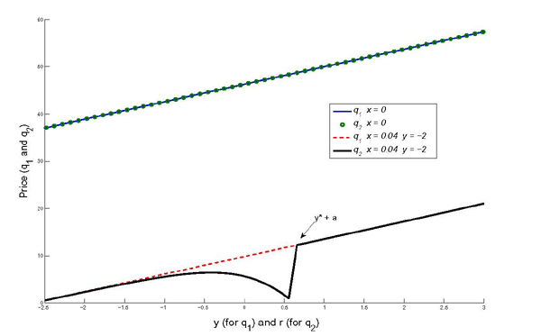
This figure displays the pricing
functions in the numerical example with continuous earnings,
computed using Simulated Annealing. The horizontal axis is revealed
previous earnings ![]() for period 1's price
for period 1's price
![]() and first-period earnings report
and first-period earnings report
![]() for period 2's price
for period 2's price ![]() .
. ![]() is the probability that the manager is
able to manipulate earnings in one period.
is the probability that the manager is
able to manipulate earnings in one period. ![]() is the
actual earnings in period 2 of the last revelation
cycle.
is the
actual earnings in period 2 of the last revelation
cycle.
With earnings management opportunity, the price of period 1 and
that of period 2 differ only to reflect the additional information
coming from the comparison between ![]() and
and
![]() . In period 2, the comparison between
. In period 2, the comparison between
![]() and
and ![]() reveals some
information about the possibility that
reveals some
information about the possibility that ![]() is a false
report, as shown in (14). Note that
is a false
report, as shown in (14). Note that ![]() is the conditional mean of the true earnings, which is
a function of
is the conditional mean of the true earnings, which is
a function of ![]() . If
. If ![]() is very small, it
is unlikely that the report has been inflated. If
is very small, it
is unlikely that the report has been inflated. If ![]() is very large, it cannot be a manipulated report because there is
no incentive to manage earnings when true earnings are greater than
is very large, it cannot be a manipulated report because there is
no incentive to manage earnings when true earnings are greater than
![]() . In particular, if
. In particular, if ![]() , the investors can infer (with probability
, the investors can infer (with probability
![]() ) that
) that ![]() is a truthful
report. In the medium range of
is a truthful
report. In the medium range of ![]() , the probability
is large that
, the probability
is large that ![]() is a false report.
is a false report.
In the particular case with normal distributions of earnings, the following result holds.
Lemma 2 if
![]() or
or
![]() ,
, ![]() is strictly decreasing in
is strictly decreasing in ![]() .
.
Proof: See Appendix.
Figure 6. Pricing Function in Period 2
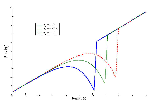
This figure displays the period-2
pricing function
![]() for different values of
for different values of
![]() . The prices are computed using Simulated
Annealing.
. The prices are computed using Simulated
Annealing. ![]() is the actual earnings in period 2 of
the last revelation cycle.
is the actual earnings in period 2 of
the last revelation cycle. ![]() is the manager's
report in period 1 of the current revelation cycle.
is the manager's
report in period 1 of the current revelation cycle.
In Figure 6, period 2's price is plotted
as a function of reported earnings for different levels of
previously revealed earnings ![]() . The dark, light,
and dashed line represent a relatively low, medium, and high level
of previous earnings respectively. If the previously revealed
earnings are higher, the threshold level that induces truthful
reporting is thus higher. The sharp drop-off of prices occurs at a
higher level of reports.
. The dark, light,
and dashed line represent a relatively low, medium, and high level
of previous earnings respectively. If the previously revealed
earnings are higher, the threshold level that induces truthful
reporting is thus higher. The sharp drop-off of prices occurs at a
higher level of reports.
5 Quantitative Results
In this section I describe how I calibrate the model. Because this model describes individual stock returns, the calibration strategy is to simulate realizations of productivity shocks and earnings management opportunities for a large number of individual firms, gather the return sequences together, and then set the parameter values so as to match the aggregate targets.
To capture fluctuations in stock market indices, the calibrated
model incorporates aggregate uncertainty: an aggregate productivity
shock. The production process that individual firms follow is thus
specified as
![]() , where
, where
![]() and
and
![]() .
Here,
.
Here,
![]() and
and
![]() represent aggregate
productivity shock and idiosyncratic productivity shock
respectively, and they are independent. Aggregate productivity
shock is assumed to be observable to both managers and investors.
In doing so, I maintain the focus on the asymmetric information
between managers and investors regarding idiosyncratic performance,
without causing additional inference problems.29
represent aggregate
productivity shock and idiosyncratic productivity shock
respectively, and they are independent. Aggregate productivity
shock is assumed to be observable to both managers and investors.
In doing so, I maintain the focus on the asymmetric information
between managers and investors regarding idiosyncratic performance,
without causing additional inference problems.29
In the rest of this section, I first calibrate the model using Compustat industrial quarterly data after restatement corrections as actual earnings process, and investigate the statistical properties of returns generated from the model.30 This case represents the benchmark calibration. Second, counterfactual experiments are conducted by considering different levels of earnings management prevalence to assess the impact of earnings management in financial markets.
5.1 Benchmark Calibration
Table 5 contains the
benchmark parameter values. The period length is set to be half a
year. The annual periodicity of restatements is thus in accordance
with the empirical finding that the average number of restated
fiscal quarters is about four (Wu, 2002).31 The discount factor ![]() is chosen to be 0.98 so that the implied semiannual real interest rate is 2
percent.
is chosen to be 0.98 so that the implied semiannual real interest rate is 2
percent.
The autoregressive parameter ![]() , the constant
drift
, the constant
drift ![]() , and standard deviations of productivity
shocks
, and standard deviations of productivity
shocks
![]() and
and
![]() are calibrated using Compustat
data. I include all available observations on the quarterly
industrial Compustat database from Q1 1971 to Q4 2006 to study
firms' earnings. Compustat quarterly files provide data on a
restated basis. When a company reports for a new quarter and at the
same time reports different data than originally reported for the
corresponding quarter of the prior year, that data for the
corresponding quarter of the prior year is changed and said to be
restated.32 In this benchmark calibration, the
net income process from Compustat is taken as actual earnings
process.
are calibrated using Compustat
data. I include all available observations on the quarterly
industrial Compustat database from Q1 1971 to Q4 2006 to study
firms' earnings. Compustat quarterly files provide data on a
restated basis. When a company reports for a new quarter and at the
same time reports different data than originally reported for the
corresponding quarter of the prior year, that data for the
corresponding quarter of the prior year is changed and said to be
restated.32 In this benchmark calibration, the
net income process from Compustat is taken as actual earnings
process.
Table 5. Benchmark Parameterization
| Parameter | Description | Value |
|---|---|---|
| Discount factor | ||
| Autoregressive parameter | ||
| Constant term | ||
| | Std.Dev of aggregate productivity shock | |
| | Std.Dev of idiosyncratic productivity shock | |
| Earnings management prevalence | ||
| Amount of overstatement | ||
| Monetary loss for one restatement | ||
| Monetary loss for two restatements |
In the results reported here, I use the sum of net income over
both quarters (Compustat quarterly data item #69) to study firms' earnings. The results are also
computed using earnings before extraordinary items (Compustat
quarterly data item #8), and the results
are generally consistent for these two alternative measures of
earnings. The earnings data are drawn from a broad spectrum of firm
sizes, and are therefore scaled following the approach in the
literature. The earnings variable is scaled by
beginning-of-the-period market value of common equity, computed as
the close price in the end of the previous period multiplied by the
number of common shares outstanding (i.e., [one-period-lagged
Compustat quarterly data item #14]
![]() [Compustat quarterly data item
#61]). Following the convention, I
also winsorize the data at 1 percent extreme values from each tail
to reduce the impact of outliers and data errors.
[Compustat quarterly data item
#61]). Following the convention, I
also winsorize the data at 1 percent extreme values from each tail
to reduce the impact of outliers and data errors.
Table 6. Moments of Semi-Annual Scaled Earnings
| Mean | Std.Dev | Autocorr | Std.Dev of avg. earnings | |
|---|---|---|---|---|
| Scaled earnings | 0.06 | 0.21 | 0.77 | 0.12 |
This table reports the descriptive statistics of semi-annual earnings calculated as net income scaled by beginning-of-the-period market value of common equity. The sample period spans from 1971 to 2006. The data is winsorized at 1 percent extreme values from each tail. The first entry is the mean, the second entry is the total standard deviation, the third entry is the autocorrelation of the pooled sample, and the last entry is the standard deviation of the average earnings across firms.
The descriptive statistics of semiannual earnings in the sample
are presented in Table
6. I normalize
the steady-state level of actual earnings to be one, that is,
 .
The value of
.
The value of ![]() is chosen to match with the average
autocorrelation of firms' earnings, which is the third entry in
Table
6. This gives
is chosen to match with the average
autocorrelation of firms' earnings, which is the third entry in
Table
6. This gives
![]() , and
, and
![]() . The standard deviation of
aggregate productivity shock
. The standard deviation of
aggregate productivity shock
![]() is set to be 0.07 to match with the time variation of average earnings
across firms, shown in the fourth column in Table
6. As
aggregate productivity shock and idiosyncratic productivity shock
are independent of one another, given the variance of aggregate
productivity shock, the standard deviation of idiosyncratic
productivity shock is calculated to be
is set to be 0.07 to match with the time variation of average earnings
across firms, shown in the fourth column in Table
6. As
aggregate productivity shock and idiosyncratic productivity shock
are independent of one another, given the variance of aggregate
productivity shock, the standard deviation of idiosyncratic
productivity shock is calculated to be
![]() .
.
The parameter ![]() is calibrated to be 0.04, yielding an overall earnings restatement rate 2
percent. This feature is in line with the average frequency of
restatement announcements among publicly traded companies over the
period of Jan 1997 to Sep 2005 (GAO, 2002 and GAO, 2006).33 Wu
(2002) documents that the average amount of restated earnings in
her sample is -$9.8 million, while the average number
of restated quarters is 4.2.34 As the model is
calibrated on a semiannual basis, I choose the amount of
overstatement to be half of $9.8 million in
each period, that is, $4.9 million. After scaled
by average market value of listed companies and then normalized by
average scaled earnings,
is calibrated to be 0.04, yielding an overall earnings restatement rate 2
percent. This feature is in line with the average frequency of
restatement announcements among publicly traded companies over the
period of Jan 1997 to Sep 2005 (GAO, 2002 and GAO, 2006).33 Wu
(2002) documents that the average amount of restated earnings in
her sample is -$9.8 million, while the average number
of restated quarters is 4.2.34 As the model is
calibrated on a semiannual basis, I choose the amount of
overstatement to be half of $9.8 million in
each period, that is, $4.9 million. After scaled
by average market value of listed companies and then normalized by
average scaled earnings, ![]() is 0.07.
is 0.07.
To measure the monetary loss that the investors incur in the
event of earnings restatements in the model, the current paper
focuses on the average immediate market-adjusted loss in market
capitalization of restating companies, that is, $75.5 million for each restatement announcement (GAO, 2002
and GAO, 2006).35 I choose the three-trading-day
window to focus regarding the market response to the exclusion of
other factors. This measure provides a lower bound for the
financial losses the investors suffer from restatements, and the
associated result serves as a lower bound for evaluating the
importance of earnings management in financial markets. The scaled
and normalized measure for the financial loss associated with each
restatement is
![]() .
. ![]() is then
set to be 2.12.
is then
set to be 2.12.
Table 7. Comparison of Data Volatility (Benchmark Calibration)
| Standard Deviation | |
|---|---|
| Model | 0.0714 |
| Data | 0.3789 |
This table reports the the average standard deviation of returns in the model with benchmark calibration and that in the CRSP data files from 1931 to 2007.
5.2 Results
I report the simulation results on the parsimoniously
parameterized model using the benchmark calibration for ![]() firms and compare the statistical properties with S&P
500 index returns data. To get compound semiannual returns, I
obtain S&P 500 quarterly returns from CRSP quarterly files from
Jan 1931 to Dec 2007.36
firms and compare the statistical properties with S&P
500 index returns data. To get compound semiannual returns, I
obtain S&P 500 quarterly returns from CRSP quarterly files from
Jan 1931 to Dec 2007.36
Table
7
shows that relative to S&P 500 Index data, the volatility of
the model-generated data is moderately lower. Table
8
compares EGARCH estimation results from the model returns and
S&P 500 Index returns. The coefficients of the EGARCH (1,1)
model are all statistically significant beyond the 95% confidence level. Consistent with the data, the
conditional variance process is strongly persistent, although the
magnitude of ![]() coefficient is not as much as the data
show. Since the coefficient
coefficient is not as much as the data
show. Since the coefficient ![]() has a negative
value, the model displays asymmetric volatility -- negative
surprises increase volatility more than positive surprises.
has a negative
value, the model displays asymmetric volatility -- negative
surprises increase volatility more than positive surprises.
Table 8a. Comparison of EGARCH (1, 1) Estimation Results (Benchmark Calibration) - Model Data
| Model data | Coefficient | Std.Error | T-statistic |
|---|---|---|---|
| -5.0000 | 2.5890 | -1.9312 | |
| 0.5260 | 0.2454 | 2.1436 | |
| 0.0529 | 0.0235 | 2.2474 | |
| -0.0234 | 0.0139 | -1.6784 |
Table 8b. Comparison of EGARCH (1, 1) Estimation Results (Benchmark Calibration) - S&P 500 Data
| S&P 500 data | Coefficient | Std.Error | T-statistic |
|---|---|---|---|
| -1.2262 | 0.5087 | -2.4105 | |
| 0.7034 | 0.1239 | 5.6773 | |
| 0.4469 | 0.1806 | 2.4742 | |
| -0.1801 | 0.1030 | -1.7479 |
This table reports the estimates of
the EGARCH coefficients in the benchmark calibration. Maximum
likelihood is used to estimate the coefficients needed to fit the
following EGARCH model to the model return series:
![]() , where
, where
![]() is an innovation and
is an innovation and
![]() is the conditional variance of
the innovation. The model return is simulated for 10,000 periods.
The S&P 500 index returns are compounded using CRSP quarterly
files from 1931 to 2007.
is the conditional variance of
the innovation. The model return is simulated for 10,000 periods.
The S&P 500 index returns are compounded using CRSP quarterly
files from 1931 to 2007.
The intuition for the EGARCH effect in the binary example with two levels of earnings can be extended to the current model with a continuum of earnings. The general unifying story is that earnings management goes hand-in-hand with weak performance, because the financial incentive to artificially inflate earnings is strong when the earnings realization is poor. Relatively low earnings lead to more frequent future restatements than high earnings, generating greater movements in the return data. The return volatility becomes state-dependent, and the state (actual earnings) is persistent. Return volatility is thus persistent and asymmetric. In addition to this direct impact, an indirect effect due to suspicion of earnings management amplifies the persistence and asymmetry in return volatility. As shown in Figure 6, the possibility of earnings management creates a region of reports at the lower end that cause active learning and intensive suspicion of misstatement. Investors lower the price in anticipation of restatements. The uncertainty regarding the firm's fundamental value and subsequent outcomes is increased in this case, and some of the earnings reports under suspicion are associated with subsequent restatements and market fluctuations. Because the reported numbers tend to persist, the volatility also persists and exhibits asymmetry.
Although the model is consistent with volatility clustering and
asymmetric volatility in the data, the magnitude is somewhat
smaller. The ![]() coefficient and
coefficient and ![]() coefficient in S&P 500 Index returns are an order of magnitude
greater than can be reproduced in the model. In light of the
difficulties in measuring monetary losses in the event of earnings
restatements, the discrepancy is not as large as it appears. For
example, GAO (2002) and GAO (2006) show that restatement
announcements have a negative effect on stock prices beyond their
immediate impact. They find persistent market capitalization
declines for restating companies. After controlling for the
movement in the overall market, they report an average of
$79.3 million loss in market value from 20
trading days before through 20 trading days after a restatement
announcement (the intermediate impact) and an average of
$136.1 million loss in market value from 60
trading days before through 60 trading days after the announcement
(the longer-term impact). In addition, the use of market
capitalization loss as a proxy for monetary loss that the investors
incur precludes other potentially important factors.37 The
effects of such errors would be to bias the financial loss
downwards, a correction of which would result in the model moving
closer to the data. Measurement errors in the frequency of earnings
management would have a similar effect on dynamic return patterns.
Another plausible explanation for the discrepancy between model
prediction and observational data is the oversimplicity of the
model. Thus, although the overall fit of the model is good, it is
not surprising, given the level of abstraction, that there are
elements of the fine structure of returns the model is not designed
to capture.
coefficient in S&P 500 Index returns are an order of magnitude
greater than can be reproduced in the model. In light of the
difficulties in measuring monetary losses in the event of earnings
restatements, the discrepancy is not as large as it appears. For
example, GAO (2002) and GAO (2006) show that restatement
announcements have a negative effect on stock prices beyond their
immediate impact. They find persistent market capitalization
declines for restating companies. After controlling for the
movement in the overall market, they report an average of
$79.3 million loss in market value from 20
trading days before through 20 trading days after a restatement
announcement (the intermediate impact) and an average of
$136.1 million loss in market value from 60
trading days before through 60 trading days after the announcement
(the longer-term impact). In addition, the use of market
capitalization loss as a proxy for monetary loss that the investors
incur precludes other potentially important factors.37 The
effects of such errors would be to bias the financial loss
downwards, a correction of which would result in the model moving
closer to the data. Measurement errors in the frequency of earnings
management would have a similar effect on dynamic return patterns.
Another plausible explanation for the discrepancy between model
prediction and observational data is the oversimplicity of the
model. Thus, although the overall fit of the model is good, it is
not surprising, given the level of abstraction, that there are
elements of the fine structure of returns the model is not designed
to capture.
5.3 Counterfactual Experiment
GAO (2002) and GAO (2006) document a significant upward trend in
the number of restatements over time. To gain insight on
policy-related issues, it is of interest to examine how the
magnitude of financial anomalies varies with the extent of earnings
management. Here, I consider the economies with different levels of
earnings management prevalence. Specifically, I consider various
values of ![]() to assess the importance of earnings
management. In these economies with different values of
to assess the importance of earnings
management. In these economies with different values of ![]() , the other parameters are chosen to match the same
aggregate targets as in the benchmark calibration.
, the other parameters are chosen to match the same
aggregate targets as in the benchmark calibration.
Table 9a. EGARCH(1,1) estimation results
with different levels of ![]() -
- ![]() =0
=0
| Coefficient | Std.Error | T-statistic | |
|---|---|---|---|
| -4.9882 | 0.6962 | -7.1651 | |
| 0.0028 | 0.7555 | 0.0037 | |
| 0.0116 | 0.0279 | 0.4133 | |
| 0.0009 | 0.0007 | 1.2500 |
Table 9b. EGARCH(1,1) estimation results
with different levels of ![]() -
- ![]() =0.04
=0.04
| Coefficient | Std.Error | T-statistic | |
|---|---|---|---|
| -5.0000 | 2.5890 | -1.9312 | |
| 0.5260 | 0.2454 | 2.1436 | |
| 0.0529 | 0.0235 | 2.2474 | |
| -0.0234 | 0.0139 | -1.6784 |
Table 9c. EGARCH(1,1) estimation results
with different levels of ![]() -
- ![]() =0.1
=0.1
| Coefficient | Std.Error | T-statistic | |
|---|---|---|---|
| -2.9453 | 1.6996 | -1.7330 | |
| 0.6786 | 0.1855 | 3.6589 | |
| 0.0353 | 0.0203 | 1.7393 | |
| -0.0255 | 0.0129 | -1.9729 |
This table reports the estimates of
the EGARCH coefficients for the model with different values of
![]() . The other parameters are recalibrated to
match the same targets. Maximum likelihood is used to estimate the
coefficients needed to fit the following EGARCH model to the model
return series:
. The other parameters are recalibrated to
match the same targets. Maximum likelihood is used to estimate the
coefficients needed to fit the following EGARCH model to the model
return series:
![]() , where
, where
![]() is an innovation and
is an innovation and
![]() is the conditional variance of
the innovation. The model return is simulated for 10,000 periods.
is the conditional variance of
the innovation. The model return is simulated for 10,000 periods.
![]() is the probability that the manager is
able to manipulate earnings in one period.
is the probability that the manager is
able to manipulate earnings in one period.
Table 9 presents the results.
The extreme case of ![]() in this model, shown in
the first panel, corresponds to the standard Lucas asset-pricing
model. In this case, earnings management does not exist. The
estimated EGARCH coefficients are substantially reduced and
insignificant. No long-memory persistence or asymmetric behavior is
present in the model data.
in this model, shown in
the first panel, corresponds to the standard Lucas asset-pricing
model. In this case, earnings management does not exist. The
estimated EGARCH coefficients are substantially reduced and
insignificant. No long-memory persistence or asymmetric behavior is
present in the model data.
As ![]() is increased to 0.04 as
in the calibrated model, the EGARCH estimation results on the
simulated return data demonstrate the presence of strong
persistence and asymmetry in volatility. When
is increased to 0.04 as
in the calibrated model, the EGARCH estimation results on the
simulated return data demonstrate the presence of strong
persistence and asymmetry in volatility. When ![]() ,
, ![]() and
and ![]() coefficients
become larger in magnitude and more significant. These are strong
indications that incorporating earnings management intensifies both
persistence and asymmetry in return volatility.
coefficients
become larger in magnitude and more significant. These are strong
indications that incorporating earnings management intensifies both
persistence and asymmetry in return volatility.
Table 10. Volatility of the Model Returns
with Different Level of ![]()
| Standard Deviation | |
|---|---|
| 0 | 0.0424 |
| 0.04 | 0.0714 |
| 0.1 | 0.1044 |
This table reports the standard
deviation of the calibrated model returns for different ![]() .
. ![]() is the probability that the manager is
able to manipulate earnings in one period.
is the probability that the manager is
able to manipulate earnings in one period.
Table
10
contains the standard deviation of returns in the simulated data.
Consistent with the empirical studies mentioned in Section
1 and Section 3.2, as
![]() increases (implying that the
informativeness of earnings reports becomes weakened), the returns
exhibit greater volatility. Monetary penalties charged upon
restatement announcements generate large swings in the return
sequence, and hence raise volatility.
increases (implying that the
informativeness of earnings reports becomes weakened), the returns
exhibit greater volatility. Monetary penalties charged upon
restatement announcements generate large swings in the return
sequence, and hence raise volatility.
Models such as the one considered in this paper can be used to predict the consequence of a particular corporate governance rule on financial reporting. The comparison of the financial returns dynamics with different prevalence of earnings management underscores why earnings management is of central importance in pricing of financial assets, in understanding the risk implied by empirical anomalies, and in the current debate about advantages of strict implementation of corporate governance policy, such as the Sarbanes-Oxley Act.
6 Robustness Check
In this section, robustness check of the baseline model is conducted, both in terms of quantitative evaluations and model specifications. First, following an alternative calibration strategy, I recalibrate the model to Compustat Unrestated data, and study the return patterns. Second, I consider a setting in which investigations are conducted stochastically, and check whether model dynamics are robust to a stochastic feature of revelations.
6.1 Alternative Calibration
Of particular interest is the sensitivity of the quantitative results to the specification of restated data as true earnings. An alternative to the benchmark calibration strategy is to take unrestated data and match them with the reported earnings generated from the model. In contrast to the conventional Compustat quarterly dataset that contains restated statements, Compustat Unrestated dataset covers the initial 10Q filing for a quarter that may be subject to SEC filings and earnings restatements in subsequent quarters. Here, I recalibrate the model using the Compustat Unrestated dataset.
Table 11. Moments of Semi-Annual Scaled Reports
| Mean | Std.Dev | Autocorr | Std.Dev of avg. | Avg. of Std.Dev | |
|---|---|---|---|---|---|
| Scaled reports | 0.10 | 0.22 | 0.82 | 0.03 | 0.15 |
This table reports the descriptive statistics of reported earnings in the Compustat Unrestated dataset from 1987 to 2006. The data is winsorized at 1 percent extreme values from each tail. The net income is scaled by beginning-of-the-period market value of common equity. The first entry is the mean, the second entry is the total standard deviation, the third entry is the autocorrelation of the pooled sample, the fourth entry is the standard deviation of the average reports across firms, and the last entry is the average standard deviation of the reports within the firms.
Table 12. Alternative Parameterization
| Parameter | Description | Value |
|---|---|---|
| ρ | Autoregressive parameter | 0.82 |
| k | Constant term | 0.18 |
| σa | Std. Dev of aggregate productivity shock | 0.02 |
| σi | Std.Dev of idiosyncratic productivity shock | 0.08 |
| β | Discount factor | 0.98 |
| x | Earnings management prevalence | 0.04 |
| α | Amount of overstatement | 0.03 |
| F1 | Monetary loss for one restatement | 0.49 |
| F2 | Monetary loss for two restatements | 0.98 |
The Compustat Unrestated dataset starts in 1987 for U.S.
companies, covering a shorter time span than the Compustat restated
dataset. Table
11 presents the
moments of semiannual reported earnings scaled by
beginning-of-the-period market value. Here, ![]() ,
,
![]() , and
, and
![]() are calibrated to match the
average autocorrelation of firms' earnings, time variation of
average reports across firms, and average time variation of reports
within firms, shown in the third, fourth, and fifth entry
respectively in Table 11. This gives
are calibrated to match the
average autocorrelation of firms' earnings, time variation of
average reports across firms, and average time variation of reports
within firms, shown in the third, fourth, and fifth entry
respectively in Table 11. This gives
![]() , and
, and
![]() . As the steady-state
report is normalized to 1,
. As the steady-state
report is normalized to 1, ![]() is then
set to be 0.18.
is then
set to be 0.18.
Table 13a. Comparison of EGARCH (1,1) Estimation Results (Alternative Calibration) - Model Data
| Model data | Coefficient | Std.Error | T-statistic |
|---|---|---|---|
| -2.7503 | 1.4893 | -1.8467 | |
| 0.8049 | 0.1056 | 7.6225 | |
| 0.0339 | 0.0166 | 2.0492 | |
| -0.0231 | 0.0106 | -2.1911 |
Table 13b. Comparison of EGARCH (1,1) Estimation Results (Alternative Calibration) - S&P 500 Data
| S&P 500 data | Coefficient | Std.Error | T-statistic |
|---|---|---|---|
| -1.2262 | 0.5087 | -2.4105 | |
| 0.7034 | 0.1239 | 5.6773 | |
| 0.4469 | 0.1806 | 2.4742 | |
| -0.1801 | 0.1030 | -1.7479 |
This table reports the estimates of
the EGARCH coefficients in the alternative calibration. Maximum
likelihood is used to estimate the coefficients needed to fit the
following EGARCH model to the model return series:
![]() , where
, where
![]() is an innovation and
is an innovation and
![]() is the conditional variance of
the innovation. The model return is simulated for 10,000 periods.
The S&P 500 index returns are compounded using CRSP quarterly
files from 1931 to 2007.
is the conditional variance of
the innovation. The model return is simulated for 10,000 periods.
The S&P 500 index returns are compounded using CRSP quarterly
files from 1931 to 2007.
The rest of the parameters are chosen to match the same targets
as in the benchmark calibration, and that gives
![]() , and
, and
![]() , as presented in Table 12. Some
values are different from the benchmark calibration because of the
normalization of reported earnings to unity, compared with the
normalization of restated earnings to unity.
, as presented in Table 12. Some
values are different from the benchmark calibration because of the
normalization of reported earnings to unity, compared with the
normalization of restated earnings to unity.
Table
13
contains measures of EGARCH effect for the model returns and
S&P 500 Index returns. The results are similar to those with
the benchmark parameterization, except that the ![]() coefficient somewhat overshoots. The stronger persistence in
volatility than in the benchmark calibration is attributable to the
higher persistence in firms' earnings. This result confirms that
most of the volatility clustering in the model has to come from the
persistent component in earnings management, which directly stems
from the persistent component in earnings. This element of the
model is crucial in making it consistent with the observed
heteroskedasticity. The finding that EGARCH effect is quite similar
for different calibration strategies suggests that, even though the
parameters may differ across economies, the nature of return
dynamics can still be quite similar.
coefficient somewhat overshoots. The stronger persistence in
volatility than in the benchmark calibration is attributable to the
higher persistence in firms' earnings. This result confirms that
most of the volatility clustering in the model has to come from the
persistent component in earnings management, which directly stems
from the persistent component in earnings. This element of the
model is crucial in making it consistent with the observed
heteroskedasticity. The finding that EGARCH effect is quite similar
for different calibration strategies suggests that, even though the
parameters may differ across economies, the nature of return
dynamics can still be quite similar.
Table 14. Comparison of Data Volatility (Alternative Calibration)
| Standard Deviation | |
|---|---|
| Model | 0.0300 |
| Data | 0.3789 |
This table reports the the average standard deviation of returns in the model with benchmark calibration and that in the CRSP data files from 1931 to 2007.
Table 14 compares the volatility of the model and the data. Compared with the benchmark parameterization, the model volatility is reduced. The reason is that the value of monetary loss associated with earnings management is calibrated to be lower (in particular, less than half in size), leading to a more moderate reaction of asset returns to restatement announcements. A smaller fluctuation of the returns during restatements produces lower volatility.
6.2 Stochastic Investigation
In the baseline model, the periodic investigation is conducted
deterministically every two periods. To examine how this assumption
affects the results, here I consider a setting where investigations
take place stochastically. As in Section 2 and
Section 3, there are two levels of earnings:
![]() . Actual earnings follow a
Markov process
. Actual earnings follow a
Markov process
The investigation regarding financial reporting is now assumed to
be stochastic, and occurs with probability ![]() every period. If the investigation takes place, all the previous
earnings since the most recent investigation are revealed. The
financial statements in the corresponding periods when earnings
management occurs have to be restated, and the investors bear
monetary penalties. More specifically, the amount of financial
charges upon restatement announcements is a strictly increasing
function of the number of periods in which the manager manipulates
earnings. The timeline of the model events in each period is
described in Figure 7.
every period. If the investigation takes place, all the previous
earnings since the most recent investigation are revealed. The
financial statements in the corresponding periods when earnings
management occurs have to be restated, and the investors bear
monetary penalties. More specifically, the amount of financial
charges upon restatement announcements is a strictly increasing
function of the number of periods in which the manager manipulates
earnings. The timeline of the model events in each period is
described in Figure 7.
Note that the derivation of the posterior probability of having a false report at each point in time requires utilizing the entire history of reports since the most recent investigation up to the current report. In particular, when the manager makes an earnings announcement every period, the investors not only infer the current realization and predict future earnings, but also revise their expectation on each previous report in history.
Figure 7. Model Timeline with Stochastic Investigation
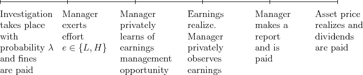
Fortunately, in this setting all the relevant information in the reporting history can be summarized with a small set of state variables. In what follows, the problem is reduced to a variational problem in which history dependence can be summarized and asset price can be characterized by the following five state variables.38
 : the conditional probability (with
the information from the current report) that the current true
earnings are high;
: the conditional probability (with
the information from the current report) that the current true
earnings are high; : the expected number of periods involving
earnings management since the last investigation until the most
recent low report (
: the expected number of periods involving
earnings management since the last investigation until the most
recent low report ( if there is no low report
since the last investigation until the previous period);
if there is no low report
since the last investigation until the previous period); : the number of consecutive high reports
until the previous period since the last low report or the last
investigation, whichever is more recent;
: the number of consecutive high reports
until the previous period since the last low report or the last
investigation, whichever is more recent; : the current earnings report,
 ;
; : the true earnings before the series
of consecutive
: the true earnings before the series
of consecutive  high reports starts.
Given the earnings management incentive in this binary setting,
the current true earnings are revealed under two circumstances. The
first is when the investigation regarding financial reporting takes
place. In this case, the entire history of earnings realizations is
revealed. The second is when the manager sends a low report. If the
reported earnings are low, although the credibility of financial
statements in prior periods remains ambiguous, the current earnings
are low with certainty. In the following, I derive the pricing
functions that describe a stationary solution to the problem using
these state variables. The stock price at time ![]() is denoted by
is denoted by
![]() .
.
Let the monetary penalties charged for earnings management be a
linear function of the number of restating periods upon
investigation. Specifically, the fines
![]() , where
, where ![]() is
a constant and
is
a constant and ![]() is the number of periods involving
earnings management since the most recent investigation. As the
investors update their beliefs in the standard Bayesian fashion,
is the number of periods involving
earnings management since the most recent investigation. As the
investors update their beliefs in the standard Bayesian fashion,
![]() evolves following Bayes'
Rule:
evolves following Bayes'
Rule:
![\begin{displaymath} % latex2html id marker 395 \gamma\prime= \begin{cases} \dfrac{\gamma\pi_{hh}+(1-\gamma)\pi_{lh}}{\gamma\pi_{hh}+(1-\gamma)\pi _{lh}+\gamma(1-\pi_{hh})x+(1-\gamma)(1-\pi_{lh})x}, & \text{$r=$}\tilde {h}\text{ at }t+1\text{,}\\ [15pt] 0, & \text{$r=$}\tilde{l}\text{ at }t+1. \end{cases}\end{displaymath}](img3a.gif)
First, the price associated with a high report,
![]() , is
derived.39
, is
derived.39
![$\displaystyle P(\gamma, Z, N, \tilde h, \bar y)=\tilde h+\beta\left[ (1-\lambda)W_{n}^{\tilde h} + \lambda W_{i}^{\tilde h} \right] .$](img565.gif) |
(16) |
Here, ![]() is the discount factor.
is the discount factor.
![]() represents the expected
price if the investigation does not occur in the beginning of the
next period, and
represents the expected
price if the investigation does not occur in the beginning of the
next period, and
![]() represents the expected
price if the investigation occurs. Both prices are conditional on a
current high report.
represents the expected
price if the investigation occurs. Both prices are conditional on a
current high report.
If the investigation does not take place in the beginning of the next period, the expected price is
| (17) |
The first term in (19) is the expected price if
the next report is high. The second term is the expected price when
the report in the next period is low. Note that a low report is
always truthful, and thus ![]() is updated to
0.
is updated to
0. ![]() denotes the conditional probability that
the manager makes a high report in the next period:
denotes the conditional probability that
the manager makes a high report in the next period:
If the investigation takes place in the next period, the expected price is
|
|
(18) |
![$\displaystyle + \gamma\left[ \xi_{1} P\left( \frac{\pi_{hh}}{\xi_{1}},0,0,\tilde h,h \right) + (1-\xi_{1}) P(0,0,0,\tilde l,h) \right]$](img575.gif)
![$\displaystyle + (1-\gamma)\left[ \xi_{2} P\left( \frac{\pi_{lh}}{\xi_{2}},0,0,\tilde h,l \right) + (1-\xi_{2}) P(0,0,0,\tilde l,l) \right] .$](img576.gif)
where ![]() represents the conditional
probability of having a high report in the next period, given the
current true earnings are high.
represents the conditional
probability of having a high report in the next period, given the
current true earnings are high. ![]() is the
probability of having a high report conditional on that the current
true earnings are low.
is the
probability of having a high report conditional on that the current
true earnings are low.
The first term in (18) is the expected amount
of financial penalties for earnings management.
![]() denotes the expected number of
falsified reports among the
denotes the expected number of
falsified reports among the ![]() consecutive
reports of high earnings since the last low report or the last
investigation, whichever is more recent. The function
consecutive
reports of high earnings since the last low report or the last
investigation, whichever is more recent. The function
![]() is calculated from the model
fundamental in a recursive manner, and the method is illustrated in
Appendix C. The number of the expected restating periods is thus
the sum of
is calculated from the model
fundamental in a recursive manner, and the method is illustrated in
Appendix C. The number of the expected restating periods is thus
the sum of
![]() and the expected number of
periods involving earnings management from the last investigation
through the most recent low report,
and the expected number of
periods involving earnings management from the last investigation
through the most recent low report, ![]() . Recall that
. Recall that
![]() is the conditional probability that
the current high report is truthful. The second term in (18) thus represents the expected price if the current
high report is truthful. The third term is the case in which the
current earnings are low and have been overstated.
is the conditional probability that
the current high report is truthful. The second term in (18) thus represents the expected price if the current
high report is truthful. The third term is the case in which the
current earnings are low and have been overstated.
Now let us consider the asset price if the current report is low.
![$\displaystyle P(0,Z,N,\tilde l,\bar y)=\tilde l +\beta\left[ (1-\lambda )W_{n}^{\tilde l} + \lambda W_{i}^{\tilde l} \right] .$](img589.gif) |
(19) |
where
![]() and
and
![]() represent the expected
price if the investigation does not occur in the next period and
the expected price if the investigation occurs, respectively,
conditional on a current low report.
represent the expected
price if the investigation does not occur in the next period and
the expected price if the investigation occurs, respectively,
conditional on a current low report.
If the investigation does not take place in the next period, the expected price is
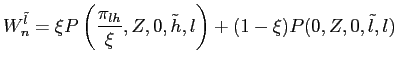
where ![]() denotes the conditional probability that
the manager makes a high report in the next period:
denotes the conditional probability that
the manager makes a high report in the next period:
If the investigation takes place in the next period:
|
(20) |
The first term in (20) is the expected monetary
charges for earnings management, which is a linear function of the
expected number of restating periods. The second term is the
expected price if the realization of actual earnings is high in the
next period, and the third term corresponds to the case in which
the realization is low. Thus, from
(16)
and
(19),
the price in each period can be solved recursively.
Table 15. Parameter Values in the Numerical Example with Binary Earnings
| Parameter | Value |
|---|---|
Table 15 contains the
parameter values. The pricing functions are computed numerically.
Figure 8 displays
![]() , the shape of which may vary
with parameterizations. Figure 9 and Figure 10 show how the prices associated with a high
report change with
, the shape of which may vary
with parameterizations. Figure 9 and Figure 10 show how the prices associated with a high
report change with ![]() and
and ![]() .
As the monetary penalties associated with earnings management is a
linear function of the number of restated financial statements, the
price in response to a high report is linearly increasing in
.
As the monetary penalties associated with earnings management is a
linear function of the number of restated financial statements, the
price in response to a high report is linearly increasing in
![]() and linearly decreasing in
and linearly decreasing in
![]() . As shown in Figure 11, the price in response to a low report is also
linearly decreasing in both
. As shown in Figure 11, the price in response to a low report is also
linearly decreasing in both ![]() , with
, with ![]() updated to 0.
updated to 0.
The model is simulated for 10,000 periods. in a numerical
example. In order to illustrate the influence of earnings
management incentive on dynamic return patterns, I compare the
model returns with ![]() and those with
and those with
![]() . Table 16 presents the EGARCH estimation results on the model returns. In a
model without earnings management (
. Table 16 presents the EGARCH estimation results on the model returns. In a
model without earnings management (![]() ), there is
no persistence in return volatility (shown in the upper panel). As
earnings management becomes possible, the coefficients of the
EGARCH model are all statistically significant. Persistence and
asymmetry are present in the model return volatility. In addition,
Table 17 shows that the model
returns become more volatile as
), there is
no persistence in return volatility (shown in the upper panel). As
earnings management becomes possible, the coefficients of the
EGARCH model are all statistically significant. Persistence and
asymmetry are present in the model return volatility. In addition,
Table 17 shows that the model
returns become more volatile as ![]() increases. The
same set of results and intuition from the model with deterministic
monitoring carry through.
increases. The
same set of results and intuition from the model with deterministic
monitoring carry through.
Figure 8. The Expected
Number of Inflated Reports Among ![]() Consecutive High
Reports
Consecutive High
Reports
![]()
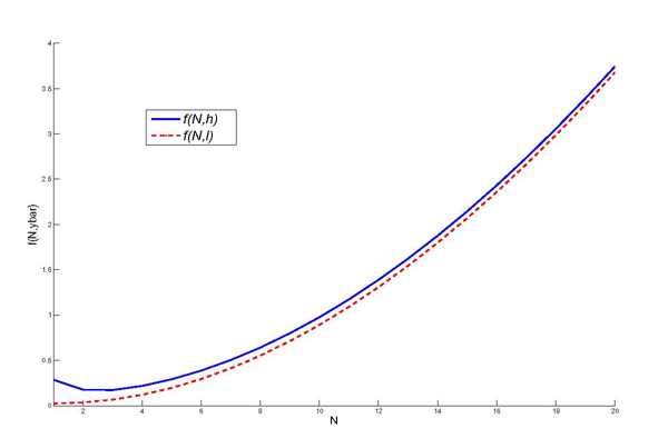
Figure 9. Price for a High
Report as a Function of ![]()
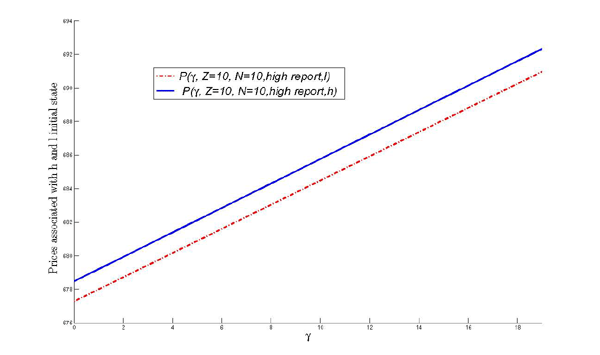 Figure 10. Price for a
High Report as a Function of
Figure 10. Price for a
High Report as a Function of ![]()
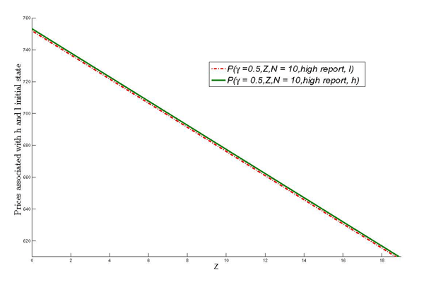
Figure 11. Price for a Low
Report as a Function of ![]()
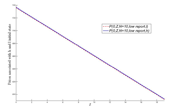
Table 16a. EGARCH (1,1) Estimation Results - ![]() =0
=0
| Coefficient | Std.Error | t-statistic | |
|---|---|---|---|
| -5.0000 | 12.8300 | -0.3897 | |
| 0.0576 | 0.0880 | 0.6552 | |
| 0.0033 | 0.0119 | 0.2838 | |
| 0.0041 | 0.0066 | 0.6195 |
Table 16b. EGARCH (1,1) Estimation Results - ![]() =0.1
=0.1
| Coefficient | Std.Error | t-statistic | |
|---|---|---|---|
| -2.0291 | 0.2979 | -6.8092 | |
| 0.7441 | 0.0376 | 19.7951 | |
| 0.1068 | 0.0207 | 5.1616 | |
| -0.0841 | 0.0197 | -4.2789 |
Variance equation:
![]()
Table 17. Volatility of the Model Returns
| Standard Deviation | |
|---|---|
| 0 | 0.0134 |
| 0.1 | 0.0193 |
| 0.2 | 0.0201 |
This model of stochastic investigation assumes a constant exogenous probability of monitoring in every period. However, with a positive monitoring cost, it is natural to argue that monitoring would occur with a higher probability in bad times, since there tends to be little interest in investigating when the market is booming. Accounting fraud does come in waves, and is detected more intensively during market collapses. As monitoring occurs more often when the aggregate state of the economy is bad and earnings management is more prevalent, the asymmetric behavior in stock returns tends to be more pronounced. An monitoring probability that varies with the aggregate economic prospects would strengthen the mechanism illustrated in this paper, and intensify these observed features of asset returns.
7 Conclusion
This paper examines dynamic asset return patterns in an economy in which information about underlying profitabilities is obscured. An important ingredient in the current formulation of the asset-pricing problem is that executives intentionally manipulate financial information in their own best interests. Executives possess two dimensions of private information: realizations of actual earnings and realizations of earnings management opportunity. Because different combinations of these two could generate identical earnings reports, there is no strict monotonicity and hence no invertibility of the reporting function. Although the investors are fully rational, and they learn in a standard Bayesian fashion, they cannot perfectly filter out the manipulation component in the reports. Therefore, earnings management causes a pricing distortion -- honest firms are undervalued, while firms that manipulate their accounting numbers are overpriced.
This study shows that an asset-pricing model with earnings management delivers the observed features of asset return data: volatility clustering, asymmetric conditional volatility, and excess individual volatility. To the best of my knowledge, such features are not replicated by one representative-agent model without introducing complex preference structures. Formal modeling of the implication of endogenously determined earnings management behavior for dynamic return patterns is rather limited. The goal is to point out that incorporating corporate misconduct in an otherwise standard asset-pricing model can mimic a number of stylized financial facts, and earnings management may play a crucial role in price formulations in financial markets.
The quantitative analysis indicates that, in addition to generating patterns in their own stocks, earnings management by individual firms may also create the observed patterns in stock market indices regardless of the covariance effects of aggregation of reporting decisions across firms. Importantly, these effects are symptoms of inefficiency and risk, and they are likely to be more pronounced during episodes of weak economic performance when the financial incentive to inflate earnings is particularly strong. The mechanism illustrated in this paper also presents a likely source of non-fundamental volatility and financial risk.
The current model of shareholders-manager behavior in a
financial market is a simplified one. In particular, the current
analysis does not explicitly model how the manager finances the
discrepancy in the reports. As elaborated in section ![]() , leaving the source of funds outside the model is for the
purpose of simplification without causing a modeling inconsistency.
This formulation can also be viewed as a simple way of illustrating
the idea that the manager can divert resources from profitable
investment to current payout. Formulating this idea explicitly
requires a production economy with investment, and I take the
current framework as the first step towards the ultimate goal. A
full understanding of the welfare consequences is a task for future
research.
, leaving the source of funds outside the model is for the
purpose of simplification without causing a modeling inconsistency.
This formulation can also be viewed as a simple way of illustrating
the idea that the manager can divert resources from profitable
investment to current payout. Formulating this idea explicitly
requires a production economy with investment, and I take the
current framework as the first step towards the ultimate goal. A
full understanding of the welfare consequences is a task for future
research.
Bibliography
Arya, A., Glover, J., and Sunder, S. (1998). "Earnings Management and the Revelation Principle," Review of Accounting Studies, 3: 7-34.
Arya, A., Glover, J., and Sunder, S. (2003). "Are Unmanaged Earnings Always Better for Shareholders?" Accounting Horizons, 17: 111-116.
Bartha, M. E., Beavera, W. H., and Landsman, W. R. (2006). "Corporate Governance, Chief Executive Officer Compensation, and Firm Performance," Journal of Financial Economics, 51: 371-406.
Bergstresser, D. and Philippon, T. (2006). "CEO Incentives and Earnings Management," Journal of Financial Economics, 80: 511-529.
Black, F. (1976). "Studies of Stock Price Volatility Changes," Proceedings of the American Statistical Association.
Black, F. and Scholes, M. (1973). "The Pricing of Options and Corporate Liabilities," Journal of Political Economy, 81: 637-654.
Brock, W. A. (1982). "Asset Pricing in a Production Economy," The Economics of Information and Uncertainty, 1-43.
Brollerslev, T. (1986). "A Conditionally Heteroskedastic Time Series Model of Security Prices and Rate of Return Data," Review of Economics and Statistics, 59: 542-547.
Brollerslev, T., Chou, R. Y., and Kroner, K. F. (1992). "ARCH modeling in Finance," Journal of Econometrics, 52: 5-59.
Burns, N. and Kedia, S. (2006). "The Impact of Performance-based Compensation on Misreporting," Journal of Financial Economics, 79: 511-529.
Campbell, J. and Hentschel, L. (1992). "No News is Good News: An Asymmetric Model of Changing Volatility in Stock Returns," Journal of Financial Economics, 31: 281-238.
Campbell, J., Lettau, M., Malkiel, B. G., and Xu, Y. (2001). "Have Individual Stocks Become More Volatile? An Empirical Exploration of Idiosyncratic Risk," The Journal of Finance, 56: 1-43.
Cecchetti, S. G., Lam, P., and Mark, N. (2000). "Asset Pricing with Distorted Belief: Are Equity Returns Too Good to Be True?" The American Economic Review, 4: 787-805.
Christie, A. (1982). "The Stochastic Behavior of Common Stock Variance: Value, Leverage, and Interest Rate Effects," Journal of Financial Economics, 10: 407-432.
Core, J. and Larcker, D. F. (2002). "Performance Consequences of Mandatory Increases in Executive Stock Ownership," Journal of Financial Economics, 64: 317-340.
Crocker, K. and Slemrod, J. (2007). "The Economics of Earnings Manipulation and Managerial Compensation," The RAND Journal of Economics, 38: 698-713.
Detemple, J. B. (1986). "Asset Pricing in a Production Economy with Incomplete Information," The Journal of Finance, 41: 381-391.
Diebold, F. X. and Nerlove, M. (1989). "The Dynamics of Exchange Rate Volatility," Journal of Applied Econometrics, 4: 1-21.
Dye, R. (1988). "Earnings Management in An Overlapping Generations Model," Journal of Accounting Research, 26: 195-226.
Engle, R. F. (1982). "Autoregressive Conditional Heteroskedasticity with Estimates of the Variance of United Kingdom Inflation," Econometrica, 50: 987-1007.
Fama, E. F. (1965). "The Behavior of Stock Market Prices," Journal of Business, 38: 34-105.
Fama, E. F. and French, K. R. (1988). "Permanent and Temporary Components of Stock Prices," Journal of Political Economy, 96: 246-273.
Fischer, P. E. and Verrecchia, R. E. (1978). "Reporting Bias," The Accounting Review, 75: 229-245.
French, K. R., Schwert, W. G., and Stambaugh, R. F. (1987). "Expected Stock Returns and Volatility," Journal of Financial Economics, 19: 3-29.
General Accounting Office (2002). "Report to the Chairman, Committee on Banking, Housing, and Urban Affairs: Financial Statement Restatements".
General Accounting Office (2006). "Financial Restatements: Update of Public Company Trends, Market Impacts, and Regulatory Enforcement Activities".
Gorton, G. B. and He, P. (2006). "Agency-Based Asset Pricing," NBER Working Paper.
Guttman, I., Kadan, O., and Kandel, E. (2006). "A Rational Expectations Theory of Kinks in Financial Reporting," Accounting Review, 81: 811-848.
Kwon, I. and Yeo, E. (2007). "Overstatement and Rational Expectations," Working paper, SUNY at Albany and Korea Institute of Finance.
Hamao, Y., Masulis, R. W., and Ng, V. (1990). "Correlations in Price Changes and Volatility across International Stock Markets," The Society for Financial Studies, 3: 281-307.
Healy, P. M. and Wahlen, J. M. (1999). "A Review of the Earnings Management Literature and its Implications for Standard Setting," Accounting Horizon, 13: 365-383
Holthausen, R. W., Larcker, D. F., and Sloan, R. G. (1995). "Annual Bonus Schemes and the Manipulation of Earnings," Journal of Accounting and Economics, 19: 29-74
Kedia, S. and Philippon, T. (2007). "The Economics of Fraudulent Accounting," Review of Financial Studies, forthcoming.
Lacker, J. M., Levy, R. J., and Weinberg, J. A. (1990). "Incentive Compatible Financial Contracts, Asset Prices, and the Value of Control," Journal of Financial Intermediation, 1: 31-56.
Lambert, R. A. (2007). "Contracting Theory and Accounting," Journal of Accounting and Economics, 32: 3-87.
Liang, J. (2004). "Equilibrium Earnings Management, Incentive Contracts, and Accounting Standards," Contemporary Accounting Research, 21: 685-718.
Loomis, C. J. (1999). "Lies, Damned Lies, and Managed Earnings: The Crackdown is Here," Fortune, 140 (August 2): 74-92.
Lucas, R. E. (1978). "Asset Prices in an Exchange Economy," Econometrica, 46: 1429-1445.
Mandelbrot, B. (1963). "The Variation of Certain Speculative Prices," The Journal of Business, 36: 394-419.
McKee, T. E. (2005). "Earnings Management: An Executive Perspective," South-Western Educational Publishing.
Merton, R. C. (1974). "On the Pricing of Corporate Debt: The Risk Structure of Interest Rates," The Journal of Finance, 29: 449-470.
Palmrose, Z., Richardson, V. J., and Scholz, S. (2004). "Determinants of Market Reactions to Restatement Announcement," Journal of Accounting and Economics, 37: 59-89.
Rajgopal, S. and Venkatachalam, M. (2007). "Financial Reporting Quality and Idiosyncratic Return Volatility over the Last Four Decades," Working Paper, University of Washington and Duke University.
Richardson, S. A., Sloan, R. G., Soliman, M. T., and Tuna, I. (2005). "Accrual Reliability, Earnings Persistence, and Stock Prices," Journal of Accounting and Economics, 39: 437-485.
Rogers, J. L., Schrand, C., and Verrecchina, R. E. (2007). "Strategic Disclosure as An Explanation for Asymmetric Return Volatility," Working paper, The University of Chicago GSB and The Wharton School of the University of Pennsylvania.
Schwert, G. W. (1989). "Margin Requirement and Stock Volatility," Journal of Financial Services Research, 71: 421-436.
Shiller, R. J. (1981). "Do Stock Prices Move Too Much to be Justified by Subsequent Changes in Dividends," The American Economic Review, 71: 421-436.
Shimokawa, S., Suzuki, K., and Misawa, T. (2007). "An Agent-based Approach to Financial Stylized Facts," Physica A: Statistical Mechanics and its Applications, 379: 207-225.
Shin, H. S. (2003). "Disclosures and Asset Returns," Econometrica, 71: 105-133.
Shorish, J. and Spear, S. E. (2005). "Shaking the Tree: An Agency-theoretic Model of Asset Pricing," Annals of Finance, 1: 51-72.
Sun, B. (2008). "Earnings Management and Executive Compensation under Moral Hazard," Working paper, University of Virginia.
Turner, L., Dietrich, J. R., Anderson, K., and Bailey, A. J. (2001). "Accounting Restatements," Unpublished working paper, SEC.
Verrecchia, R. E. (1983). "Discretionary Disclosure," Journal of Accounting and Economics, 5: 179-194.
Wang, J (1993). "A Model of Intertemporal Asset Prices under Asymmetric Information," The Review of Economic Studies, 60: 249-282.
Wei, K. C., Liu, Y., Yang, C., and Chaung, G. (1995). "Volatility and Price Change Spillover Effects across the Developed and Emerging Markets," Pacific -Basin Finance Journal, 1: 113-136.
Wu, M. (2002). "Earnings Restatements: A Capital Market Perspective," Working Paper, The University of Hong Kong.
Appendix
A Proofs
Proof of Proposition 2:
After the parallel shift of
![]() and
and
![]() by
by ![]() ,
the conditional distribution of actual earnings given effort is
denoted by
,
the conditional distribution of actual earnings given effort is
denoted by
![]() ,
,
![]() . The principal has a
utility function given by
. The principal has a
utility function given by ![]() .
.
The Lagrangian for the principal's problem in this case is
![$\displaystyle \int_{\underline{y}+\delta}^{\bar{y}+\delta} \bigg\{ V \left[ y-w(r(y)) \right] g(y\vert e=H) + \lambda\left[ u(w)g(y\vert e=H)-\bar{U} \right]$](img660.gif) |
|
![$\displaystyle + \mu\left[ u(w) g(y\vert e=H) - u(w) g(y\vert e=L) - c \right] \bigg\} dy$](img661.gif) |
The reporting function ![]() is given by
is given by
![\begin{displaymath} % latex2html id marker 397 r(y)= \begin{cases} y+a\quad & \text{if $u\left[ w(y+a)\right] -u\left[ w(y)\right] >\psi$, and earnings management opportunity realizes}\ y\quad & \text{otherwise.} \end{cases}\end{displaymath}](img4a.gif)
Differentiating with respect to ![]() inside
the integral sign, we obtain the first-order condition. Assuming
that it is optimal to elicit high effort, an optimal incentive
compensation scheme
inside
the integral sign, we obtain the first-order condition. Assuming
that it is optimal to elicit high effort, an optimal incentive
compensation scheme ![]() satisfies
satisfies
![$\displaystyle \frac{V^{\prime}[y-w(r)]}{u^{\prime}[w(r)]} = \lambda+ \mu\left[ 1-\frac{g\left( y(r)\vert e=L \right) }{g\left( y(r)\vert e=H \right) } \right] ,$](img669.gif) |
(21) |
Assume that the principal is risk-neutral, and the manager's
utility function takes the logarithm form given by
![]() . (21)
simplifies to
. (21)
simplifies to
![$\displaystyle = \lambda+ \mu\left[ 1-\frac{g\left( y(r)\vert e=L \right) }{g\left( y(r)\vert e=H \right) } \right]$](img672.gif) |
||
![$\displaystyle = \lambda+ \mu\left[ 1-\frac{f\left( y(r)-\delta\vert e=L\right) }{f\left( y(r)-\delta\vert e=H\right) } \right]$](img673.gif) |
(22) |
The solutions also satisfy the complementary slackness conditions
which can be rewritten as
 |
(23) |
 |
(24) |
The following inequalities should also be satisfied
| (25) |
Let ![]() be the solution to the principal's
problem before the parallel shift of
be the solution to the principal's
problem before the parallel shift of
![]() and
and
![]() .
.
![]() and
and ![]() are
the corresponding Lagrangian multipliers. Then
are
the corresponding Lagrangian multipliers. Then ![]() ,
,
![]() , and
, and ![]() satisfy the first-order condition
satisfy the first-order condition
![$\displaystyle w^{*}(r) = \lambda^{*} + \mu^{*} \left[ 1-\frac{f\left( y(r)\vert e=L \right) }{f\left( y(r)\vert e=H\right) } \right]$](img687.gif) |
together with the complementary slackness conditions
and the inequalities
It follows that
![$\displaystyle w^{*}(r-\delta) = \lambda^{*} + \mu^{*} \left[ 1-\frac{f\left( y(r)-\delta\vert e=L \right) }{f\left( y(r)-\delta\vert e=H \right) } \right] $](img691.gif)
![$\displaystyle \lambda^{*} \int_{\underline{y}+\delta}^{\bar{y}+\delta} \left\{ u \left[ w^{*}(r-\delta) \right] f(y-\delta\vert e=H)-\bar{U} \right\} dy = 0, $](img692.gif)
![$\displaystyle \mu^{*} \int_{\underline{y}+\delta}^{\bar{y}+\delta} \left\{ u \left[ w^{*}(r-\delta) \right] f(y-\delta\vert e=H) - u \left[ w^{*}(r-\delta) \right] f(y-\delta\vert e=L) - c \right\} dy = 0. $](img693.gif)
It is straightforward to determine that
![]() ,
,
![]() , and
, and
![]() satisfy (22), (23), (24), and (25). The reporting
choice
satisfy (22), (23), (24), and (25). The reporting
choice ![]() remains unchanged in this case.
Therefore, a parallel shift of the wage function by
remains unchanged in this case.
Therefore, a parallel shift of the wage function by ![]() solves the principal's problem.
solves the principal's problem.
The idea underlying this analysis is that given a parallel shift of conditional distributions of output, a parallel shift of the wage payment schedule by the same amount provides the same incentive to the manager and same marginal value of effort to the risk-neutral principal. First, because the distribution of wage payment remains unchanged after parallel shifts of the wage function and output distribution by a same amount, the manager does not have an incentive to deviate from the recommended effort and reporting choice.
Second, the risk-neutral principal designs the compensation
based on the monetary value of high effort relative to low effort,
which is the difference in the residuals. The residual is the
expected earnings net of compensation payment, conditional on high
and low effort. The monetary value of effort can be denoted by
![]() expected earnings given high effort -
expected payment given high effort
expected earnings given high effort -
expected payment given high effort![]() expected
earnings given high effort
expected
earnings given high effort ![]() expected payment
given low effort
expected payment
given low effort![]() . It can be rewritten as
. It can be rewritten as
![]() expected earnings given high effort
expected earnings given high effort
![]() expected earnings given low effort
expected earnings given low effort
![]() expected payment given high effort
expected payment given high effort
![]() expected payment given low effort
expected payment given low effort
![]() . As long as
. As long as
![]() and the wage distribution
remain constant, the principal does not have any incentives to
change the shape of incentive schemes.
and the wage distribution
remain constant, the principal does not have any incentives to
change the shape of incentive schemes.
A parallel shift of the wage schedule by an equal amount as the
shift of output distributions provides the manager with the same
incentive and the principal with the same value, and therefore is
an optimal contract in this case.
Proof of Lemma 4:
If
![]() ,
,
|
||
![$\displaystyle =\frac{1}{1 + \displaystyle x \left[ \frac{f(r-a-k-\rho y)}{f(r-k-\rho y)} \right] }$](img716.gif)
|
||
![$\displaystyle =\frac{1}{1 + \displaystyle x \exp\left[ \frac{1}{2\sigma} (r-k-\rho y)^{2} - \frac{1}{2\sigma} (r-a-k-\rho y)^{2} \right] }$](img717.gif)
|
||
![$\displaystyle = \frac{1}{1 + \displaystyle x \exp\left[ \frac{a}{2 \sigma} (2r - 2 k - 2\rho y -a) \right] }$](img718.gif)
|
Using the same property of normal distributions, it is
straightforward to check that ![]() is decreasing in
is decreasing in
![]() when
when ![]() .
.
![$\displaystyle p=\frac{1}{1 + \displaystyle (1-x) \exp\left[ \frac{a}{2 \sigma} (2r - 2 k - 2\rho y -a) \right] }.$](img722.gif)
|
B Examples of State Variables in the Model with Stochastic Investigation
As the monetary penalties upon investigation depends on the
number of restated financial statements, the expected number of
periods in which the manager inflates earnings since the most
recent realization up to now is necessary in characterizing the
prices. If there are ![]() consecutive high reports
and no low reports after the most recent investigation, a function
of
consecutive high reports
and no low reports after the most recent investigation, a function
of
![]() determines the expected number
of periods involving earnings management until the last period. If
there is any low report after the last investigation, the sum of
determines the expected number
of periods involving earnings management until the last period. If
there is any low report after the last investigation, the sum of
![]() and
and
![]() summarizes the history. In
addition,
summarizes the history. In
addition, ![]() and
and ![]() incorporate
the information regarding the current true state conveyed by the
current report.
incorporate
the information regarding the current true state conveyed by the
current report.
To be clear on what each variable represents, a set of
clarifying examples is provided in the following. Now let today be
![]() and let the last investigation happen
at the beginning of
and let the last investigation happen
at the beginning of ![]() . Suppose that the true
state of
. Suppose that the true
state of ![]() is revealed to be
is revealed to be ![]() .
.
- If
 , then, at
  ,
,  is the expected
number of inflated reports during periods 5, 6, and 7;
is the expected
number of inflated reports during periods 5, 6, and 7;  (it does not include the current period); and
 .
.  ,
because the true state in period 8 is known to be low (recall that
all the low reports are honest reports).
,
because the true state in period 8 is known to be low (recall that
all the low reports are honest reports). - If
 , then, at
  ,
,  (there is not
any low report after the last investigation until the previous
period);
(there is not
any low report after the last investigation until the previous
period);  (it does not include the current
period); and
(it does not include the current
period); and
 .
.
 , because it is the known true
state before the consecutive high reports.
, because it is the known true
state before the consecutive high reports. - If
 , then, at
  ,
,  (there is not
any low report after the last investigation until the previous
period);
(there is not
any low report after the last investigation until the previous
period);  ; and
; and
 .
.
 , because it is the known true
state before the consecutive high reports. Note that
, because it is the known true
state before the consecutive high reports. Note that  at
at  , because the current low
report is an honest one.
, because the current low
report is an honest one. - If
 , then, at
  ,
,  is the expected
number of inflated reports during periods 5, 6, and 8;
is the expected
number of inflated reports during periods 5, 6, and 8;  (it does not include the current period); and
 .
.  ,
because the true state in period 9 is known to be low (all the low
reports are honest reports). Note that in the case of
,
because the true state in period 9 is known to be low (all the low
reports are honest reports). Note that in the case of  ,
,  is set to be
  (
( occurs only when the report at
 is low or the investigation happens at
the beginning of
is low or the investigation happens at
the beginning of  ).
). - If
 , then, at
  ,
,  is the expected
number of inflated reports during periods 5, 6, 7, and 8;
is the expected
number of inflated reports during periods 5, 6, 7, and 8;
 ; and
; and
 .
.  ,
because the true state in period 9 is known to be low (Again, all
the low reports are honest reports).
,
because the true state in period 9 is known to be low (Again, all
the low reports are honest reports).
Let today be ![]() and let the investigation happen
at the beginning of
and let the investigation happen
at the beginning of ![]() .
.
- If
 , then
  ,
,
 ,
,
 , and
, and
 .
. - If
 , then
  ,
,
 ,
,
 , and
, and
 .
.
C Calculation of
 in the Model with Stochastic
Investigation
in the Model with Stochastic
Investigation
Let the information set
![]() .
. ![]() represents the true earnings in period
represents the true earnings in period
![]() ,
,
![]() .
Thus
.
Thus
![]() can be written as
can be written as
The problem of deriving
![]() in a recursive way is
transformed into an equivalent problem, that is, to recursively
derive
in a recursive way is
transformed into an equivalent problem, that is, to recursively
derive
Note that
The proof includes two steps. In step 1,
![]() and
and
![]() are
calculated. In step 2, I show that
are
calculated. In step 2, I show that
![]() and
and
![]() ,
,
![]() ,
can be calculated using
,
can be calculated using
![]() and
and
![]() ,
,
![]() .
.
As the first step,
![]() and
and
![]() are
derived as follows.
are
derived as follows.
![$\displaystyle = \displaystyle \frac{\Pr[y_{1}=h,r_{1}=\tilde h\vert\bar y=l]}{\Pr[r_{1}=\tilde h\vert\bar y=l]}$](img811.gif)
|
||
|
||
![$\displaystyle = \displaystyle \frac{\Pr[y_{1}=h,r_{1}=\tilde h\vert\bar y=h]}{\Pr[r_{1}=\tilde h\vert\bar y=h]}$](img815.gif)
|
||
|
In step 2, I first show that
![]() can be calculated if
can be calculated if
![]() is
known. For
is
known. For
![]() ,
,
![$\displaystyle \Pr[y_{n}=h \vert \mathcal{R}_{N}^{l},r_{N+1}=\tilde h ] = \frac {\Pr[y_{n}=h, r_{N+1}=\tilde h\vert\mathcal{R}_{N}^{l}]}{\Pr[r_{N+1}=\tilde h \vert \mathcal{R}_{N}^{l}]}.$](img820.gif)
|
(26) |
The denominator in (26),
![]() , is derived
as the following.
, is derived
as the following.
where
| (27) |
As
![]() is
known from the supposition, this can be calculated. The denominator
is obtained
is
known from the supposition, this can be calculated. The denominator
is obtained
| (28) |
Now let us consider the numerator in (26).
For ![]() ,
,
![]() can
be rewritten as
can
be rewritten as
where
![]() is
derived in (27).
is
derived in (27).
For
![]() , the
numerator
, the
numerator
![]() can be
rewritten as
can be
rewritten as
Here,
![]() is
known from the supposition. Now we only need to check if
is
known from the supposition. Now we only need to check if
![]() can be
calculated. I rewrite
can be
calculated. I rewrite
where
| (29) |
| (30) |
If ![]() , it is straightforward to determine that
, it is straightforward to determine that
Now let us consider
![]() if
if
![]() . Because actual earnings
. Because actual earnings ![]() follow a Markov process, all the past information is fully
summarized in the most recent realization, and the prior
realizations are informationally irrelevant. Thus,
follow a Markov process, all the past information is fully
summarized in the most recent realization, and the prior
realizations are informationally irrelevant. Thus,
and
Recall that
![]() . Therefore,
. Therefore,
![\begin{displaymath} % latex2html id marker 399 \Pr[y_{N+1}=h\vert y_{n}=h,R_{N}^{l}]= \begin{cases} \Pr[y_{N-n+1}=h\vert R_{N-n}^{h}] & \text{ if }n<N\text{,}\ \pi_{hh} & \text{ if }n=N\text{.} \end{cases}\end{displaymath}](img5a.gif) |
(31) |
and
where
![]() is
known from the supposition, since
is
known from the supposition, since ![]() .
Therefore,
.
Therefore, ![]() and
and ![]() can be
both calculated. Hence, the numerator in (26)
can be derived following this procedure. The numerator is obtained
can be
both calculated. Hence, the numerator in (26)
can be derived following this procedure. The numerator is obtained
![\begin{displaymath} % latex2html id marker 401 \Pr[y_{n}=h,r_{N+1}=\tilde{h}\vert R_{N}^{l}]= \begin{cases} \pi_{hh}\Pr[y_{N}=h\vert R_{N}^{l}]+\pi_{lh}[1-\Pr[y_{N}=h\vert R_{N}^{l}]] & \text{if }n=N+1\text{,}\\ [15pt] \Pr[y_{N}=h\vert R_{N}^{l}][\pi_{hh}+x(1-\pi_{hh})] & \text{if }n=N\text{,}\\ [15pt] \Pr[y_{n}=h\vert R_{N}^{l}]\left\{ \begin{array}[c]{c} \pi_{hh}\Pr[y_{N-n}=h\vert R_{N-n}^{h}]+\ \pi_{lh}[1-\Pr[y_{N-n}=h\vert R_{N-n}^{h}]]\ +x\{1-\pi_{hh}\Pr[y_{N-n}=h\vert R_{N-n}^{h}]-\pi_{lh}[1-\Pr[y_{N-n}=h\vert R_{N-n} ^{h}]]\} \end{array}\right\} & \text{if }n<N\text{.} \end{cases}\end{displaymath}](img6a.gif) |
(32) |
Now combining the expressions (28)
and (32), it has been shown that
![]() can be
calculated using
can be
calculated using
![]() . The
same procedure can be repeated for
. The
same procedure can be repeated for
![]() as
follows.
as
follows.
![$\displaystyle \Pr[y_{n}=h \vert \mathcal{R}_{N}^{h},r_{N+1}=\tilde h ] = \frac{\Pr[y_{n}=h, r_{N+1}=\tilde h\vert\mathcal{R}_{N}^{h}]}{\Pr[r_{N+1}=\tilde h \vert \mathcal{R} _{N}^{h}]}. $](img904.gif)
where the denominator is
and the numerator is
![\begin{displaymath} % latex2html id marker 403 \Pr[y_{n}=h,r_{N+1}=\tilde{h}\vert R_{N}^{l}]= \begin{cases} \pi_{hh}\Pr[y_{N}=h\vert R_{N}^{h}]+\pi_{lh}[1-\Pr[y_{N}=h\vert R_{N}^{h}]] & \text{if }n=N+1\text{,}\\ [15pt] \Pr[y_{N}=h\vert R_{N}^{h}][\pi_{hh}+x(1-\pi_{hh})] & \text{if }n=N\text{,}\\ [15pt] \Pr[y_{n}=h\vert R_{N}^{h}]\left\{ \begin{array}[c]{c} \pi_{hh}\Pr[y_{N-n}=h\vert R_{N-n}^{h}]+\ \pi_{lh}[1-\Pr[y_{N-n}=h\vert R_{N-n}^{h}]]\ +x\{1-\pi_{hh}\Pr[y_{N-n}=h\vert R_{N-n}^{h}]-\pi_{lh}[1-\Pr[y_{N-n}=h\vert R_{N-n} ^{h}]]\} \end{array}\right\} & \text{if }n<N\text{.} \end{cases}\end{displaymath}](img7a.gif) |
Footnotes
1. I gratefully acknowledge Eric Young and Chris Otrok for their inspiration and support. A special debt of gratitude is owed to Toshi Mukoyama for meticulous guidance and to Mark Carey for enormous help. I am also greatly indebted to David Bowman, Antonio Falato, Pingyang Gao, Marvin Goodfriend, Jon Glover, Rick Green, Denis Gromb, Zhiguo He, Bob King, Pete Kyle, Nathan Larson, Richard Leftwich, Pierre Liang, Yohei Okawa, Michael Palumbo, Nagpurnanand R. Prabhala, Adriano Rampini, Steve Sharpe, Cathy Schrand, Abbie Smith, Xuan Tam, John Weinberg, Wei Xiong, and Stan Zin for their helpful comments. I sincerely thank the seminar participants at Boston University, Carnegie Mellon University, Cornell University, Darden School of Business, Federal Reserve Board of Governors, Federal Reserve Bank of Cleveland, Federal Reserve Bank of Richmond, Georgetown University, INSEAD, Peking University, University of Chicago Booth School of Business, University of Maryland, University of Virginia, Wharton School of Business, World Bank, and Tsinghua University, for their helpful comments. In addition, I thank University of Virginia, John M. Olin Foundation, and Federal Reserve Board for financial support. The views expressed herein are the author's and do not necessarily reflect the opinions of the Board of Governors of the Federal Reserve System. Return to text
2. Contact: Division of International Finance, Board of Governors of the Federal Reserve, Mail Stop 44, 20th Street and Constitution Avenue, Washington, DC 20551. [email protected]. (202)452-2343. Return to text
3. Morgan Stanley determined the accounting tactics, while legal, enabled Freddie Mac, and to a lesser extent Fannie Mae, to overstate the value of their reserves. Both companies also pushed inevitable losses into future by sharply curtailing their repurchase of soured mortgages out of the securitizations they have guaranteed. "Fannie Mae and Freddie Mac were 'playing games with their accounting' to meet reserve requirements, prompting the government to seize control of the companies," U.S. Senator Richard Shelby said (Bloomberg [September 9, 2008]). In the case of AIG, PricewaterhouseCoopers prompted an announcement about the material accounting weaknesses related to the valuation of AIG's derivatives holdings. Prosecutors insisted that five former executives from the American International Group deliberately mounted a fraud to manipulate its financial statements, after a string of AIG scandals early this decade."Accounting flaws at American International Group significantly understated the insurance giant's losses on complex financial instruments linked to mortgages and corporate debt," AIG said in an official public statement (The New York Times [February 12, 2008]). Return to text
4. I thank Min Wu for providing Figure
3 of Wu [2002], which is reproduced as Figure
![]() in the current paper. Return to text
in the current paper. Return to text
5. The modeling technique presented here bears some similarities with Shorish and Spear [2005]. The similarities and differences between their paper and this paper will be discussed later in this section. Return to text
6. This analysis does not make a
distinction between earnings management and fraud. While the
accounting choices that explicitly violate Generally Accepted
Accounting Principles (GAAP) clearly constitute both earnings
management and fraud, according to the SEC, systematic choices made
within the boundaries of GAAP can constitute earnings management as
long as they are used to obscure the true performance of a firm and
will lead to adverse consequences for the firm in the same way as
fraud.
Following this notion, there is no economic difference between
fraud and earnings management in the model: in both cases the
reported number is different from the true amount, and such
behavior hurts the firm's future prospects. Return to text
7. The notion of "restatements" in the paper does not necessarily imply actual restatement announcements but rather the broadly-defined adverse consequences of earnings management. The periodic revelations of true earnings in the model hence capture the negative consequences of earnings management that periodically show up in returns and can be understood as reflecting the reversing nature of earnings management. Return to text
8. Following Shin [2003], Rogers et al. [2007] empirically document that strategic disclosure, defined as the reporting of good news and the withholding of bad news, provides an explanation for asymmetric return volatility. They find that asymmetric volatility is more pronounced in the return series of individual firms that are more likely to disclose strategically as measured by their litigation risk incentives. Patterns in return volatility in market indices are also consistent with strategic disclosure as an explanation. As earnings management represents strategic decisions in mandatory reporting, different from strategic disclosure with verifiable reports, I do not present their findings as direct empirical evidence for this model. However, their paper suggests that financial reporting decisions can matter in generating the observed patterns in stock returns, in line with the prediction of the current model. Return to text
9. A recent paper by Crocker and Slemrod [2007] considers an alternative environment where the Revelation Principle can be applied. In solving the model, they assume a monotonically increasing reporting function; actual earnings can therefore be recovered by inverting the reporting function. In their setting, the principal knows the exact amount of actual earnings as a function of the report, while in the current model the principal faces uncertainty over whether earnings management occurs. The manager possesses a second dimension of private information in this model, and hence the reporting function is no longer invertible. As a model that constructs an explanation for earnings management, the current contract work can be viewed as complementary to theirs. As a microeconomic foundation for the investigation into asset pricing with earnings management, their model would generate prices that are fully revealing in the equilibrium; whereas the investors in this model try to infer the true outcomes through Bayesian learning, but cannot perfectly see through earnings management. Return to text
10. This analysis does not explicitly model how the manager finances the discrepancy in the reports. In reality, the manager can obtain funds from the firm's suppliers by talking them into some sham transactions or borrow money from banks. Although without the active help from suppliers and banks, companies could not have deceived investors and analysts alike, a recent Supreme Court ruling shields third parties, including suppliers and banks, from being held responsible for knowingly participating in financial data manipulation. The source of funds is therefore chosen to be left outside the model for simplification without causing any modeling inconsistencies. Return to text
11. The model results do not hinge on the particular time structure of information disclosure. The model results are robust to a stochastic nature of investigation. Return to text
12. The model lets the financial cost of earnings management almost entirely fall on the investors by dismissing the manager before the investigation, which reflects a general view that investors suffer most from earnings manipulation (please see footnote 20 for more details) whereas executives tend to absorb personal gains. While a dynamic contract with auditing technology can be an interesting extension of the model, the current version suffices in delivering overstatement in the equilibrium so as to derive its asset pricing implication. Return to text
13. Grahama et al. [2005] document that 78% of executives in the survey admit to sacrificing long-term value to maintain predictability in earnings. Return to text
14. Both as a proxy for current economic performance and an indicator of the firm's future productivity, a distinction between earnings and cash flows is not necessary in the paper. In particular, the manager inflates the reported performance, which could be earnings or, less commonly, cash flows; such manipulative behavior comes at the expense of longer term benefits, decreasing the value of future earnings and cash flows. Return to text
15. Here, whether the manager has the
opportunity of managing earnings is assumed to be a random event,
and the outcome is the manager's private information. Generally
Accepted Accounting Principles (GAAP) provide guidelines on how to
record and summarize each type of economic transaction, and hence
define the accounting latitude available to senior management in
financial reporting. In practice, certain economic activities,
those where there is no hard-and-fast rule for which accounting
method to use, lead to more discretion than others. In any
particular period, economic transactions of this type may or may
not take place. By virtue of being closer to the operations
process, only the manager knows the extent of these activities and
hence the degree of reporting latitude available.
In modeling language, the stochastic opportunity to manage
earnings adds an additional noise in financial reports that
investors cannot perfectly filter out. Due to the additional
uncertainty, the investors need to make inferences as to whether
earnings management occurs, and earnings management is not fully
unraveled in the equilibrium. Alternatively, an environment where
the opportunity to manipulate reports realizes with certainty while
the size of manipulation is stochastic would be essentially
identical to the current model. Return
to text
16. There are two frictions in the model
that restrain earnings management: earnings management opportunity
that realizes with probability ![]() and the cost
involved in misstating earnings
and the cost
involved in misstating earnings ![]() . This model can
be also considered with only one friction: the cost of manipulation
with a simple stochastic structure. The manipulation cost now in
the model follows a binary distribution with two possible
realizations
. This model can
be also considered with only one friction: the cost of manipulation
with a simple stochastic structure. The manipulation cost now in
the model follows a binary distribution with two possible
realizations ![]() and
and ![]() . The cost
of manipulating earnings includes the educational cost of learning
how to modify certain components of earnings without getting
detected, the costs involved in bribing auditors not to report a
discrepancy in the earnings report, and expected reputation damage
in case of being caught. Return to
text
. The cost
of manipulating earnings includes the educational cost of learning
how to modify certain components of earnings without getting
detected, the costs involved in bribing auditors not to report a
discrepancy in the earnings report, and expected reputation damage
in case of being caught. Return to
text
17. Following Dye [1988], the model presented in this section places restrictions on the manager's ability to communicate the truth. In addition to the unobserved effort level, the manager observes two dimensions of information, the value of actual earnings and the realization of misstatement opportunity. However, the manager is permitted to communicate only a one-dimensional signal, which is an earnings announcement. Communication is restricted in that the manager cannot fully communicate the full dimensionality of his information, and hence the Revelation Principle is not applicable. Return to text
18. As in the standard principal-agent model, the principal is the residual claimant, and hence entitled to receive the firm's earnings. The one-step departure from the standard model here is that the principal in this model does not observe the true earnings when the principal has to compensate the manager. Return to text
19. This paper has a central focus on misreporting on upside. The reason is that overstatement of earnings is more widespread than understatement in the data and more problematic in general. Empirical work on SEC enforcement actions aimed at violations of Generally Accepted Accounting Principles suggests that over-reporting is the more frequent source of firm-wide financial misrepresentation (Feroz et al. [1991]). The average amount of restated earnings is hugely negative, and over 75% of restating firms restated their earnings downwards, indicating a strong drive to appear more productive than they actually are. Burgstahler and Dichev [1997] also estimate that 8-12 percent of the firms with small pre-managed earnings decreases manipulate earnings to achieve earnings increases, and 30-44 percent of the firms with small pre-managed losses manage earnings to create positive earnings. As long as the asymmetry between overstatement and understatement remains, in other words, the magnitude, frequency and consequences of overstatement are not exactly identical to those of understatement, the model results and intuition hold. Return to text
20. If
![]() ,
the cost of earnings management is offset by its benefit exactly,
and it is straightforward to determine that prices become
independent of
,
the cost of earnings management is offset by its benefit exactly,
and it is straightforward to determine that prices become
independent of ![]() . If
. If
![]() ,
the benefit of earnings management overwhelms its cost, then
earnings management is not only beneficial to the manager, but also
to the investors. The prices increase with the frequency of
earnings management. Return to
text
,
the benefit of earnings management overwhelms its cost, then
earnings management is not only beneficial to the manager, but also
to the investors. The prices increase with the frequency of
earnings management. Return to
text
21. This is a better description of
reality than the other two cases, as indicated in the calibration
exercise. The Securities and Exchange Commission has collected over
$10 billion penalties in fraud cases since 2002, and the amount of
settlement fines has been growing over time. In addition, as a
typical yet somewhat extreme example, the meltdown of Enron caused
over 4,500 employees to lose their jobs and pension funds worth
over $1 billion. The stock's value plummeted from $90 to below 50
cents, wiping out $60 billion of shareholders' assets. The loss of
confidence in corporate financial reporting could also hurt
business and investment opportunities. Furthermore, the reduced
availability and higher cost of capital may as well cause firms to
postpone capital spending plans and accelerate layoffs. Although
the production inefficiency due to earnings restatements, including
a declaration of bankruptcy and the lack of investment caused by
reputation damage, is not specifically modeled in this framework,
it is implicitly included in the monetary losses ![]() and
and ![]() that are incurred during the
periodic investigations. Return to
text
that are incurred during the
periodic investigations. Return to
text
22. CEOs of public companies earn a mean of $600,000 this decade, which is about 0.5% of the firms' average earnings. Return to text
23. There can be asymmetry in volatility due to a denominator effect in discrete state models, which is quantitatively insignificant in the numerical example. As shown in the comparative static analysis and continuous case, the mechanism is not a result of the binary structure. Return to text
24. It is worth noting that the asset pricing model is consistent with the contract model in the sense that it is optimal for the investors to implement high effort when designing executive compensation, although earnings management leads to monetary penalties imposed on the investors. Recall that in the contract model with two-earnings-level specification, the principal always wants to induce high effort. In the following analysis, wage values are assumed to be negligibly small relative to firms' earnings. In a standard principal-agent model without earnings management, high effort is desirable as long as high earnings are different enough from low earnings. With the possibility of earnings management and revelations, it is still beneficial for the principal to induce high effort if the value of high effort outweighs the possible monetary loss associated with earnings management. That is,
| (11) |
And recall that for earnings management to exert influence on stock returns, the discounted monetary penalties associated with earnings management must be different from the amount of overstatement, and this analysis focuses on the case that earnings management is costly to the investors. That is,
| (12) |
The numerical example used here satisfies both (11) and (12). The assumption that high effort is desirable for the principal remains valid, after taking into account the negative consequence of earnings management. Return to text
25. If ![]() , then a positive
surprise (
, then a positive
surprise (
![]() ) has the same effect on
volatility as a negative surprise of the same magnitude. If
) has the same effect on
volatility as a negative surprise of the same magnitude. If
![]() , a positive surprise increases
volatility less than a negative surprise. If
, a positive surprise increases
volatility less than a negative surprise. If ![]() , a positive surprise actually reduces volatility
while a negative surprise increases volatility. For further
reference, see Hamilton [1994, p. 668]. Return to text
, a positive surprise actually reduces volatility
while a negative surprise increases volatility. For further
reference, see Hamilton [1994, p. 668]. Return to text
26. The core intuition does not hinge upon the two-period time structure of information disclosure. The mechanism that drives EGARCH property stays in effect when the model incorporates additional periods and stochastic investigation. Return to text
27. Again, the labor wage is assumed to be negligibly small compared with the firm's earnings, therefore compensation does not affect net dividends or asset prices. Return to text
28. A possible alternative interpretation of the existence of threshold level outside the model is that executives strive to beat the consensus earnings forecast by financial analysts, and the best forecast is the conditional mean of earnings given the previous earnings reports. Return to text
29. If aggregate productivity shock is unobservable to investors, earnings reports from all the firms in the economy convey information regarding the aggregate state of the economy. In pricing individual firms, investors should utilize earnings reports from all the firms to filter out aggregate shock and then make inference about individual outcomes. As earnings management is considered as a phenomenon arising from asymmetric information about idiosyncratic performance, the possible information asymmetry regarding aggregate economy is beyond the scope of this paper. Return to text
30. There is a possibility that earnings management may be more prevalent than earnings restatements, and there can be a potential discrepancy between restated earnings and true earnings. However, the model in this paper is designed to examine the impact of earnings management behavior that leads to SEC enforcement actions or earnings restatements. Thus, earnings management practice that goes unnoticed over the firm's entire life cycle is outside the scope of the model. I will also consider matching the moments of unrestated earnings later in the next section to check the robustness of model properties. Return to text
31. Wu (2002) analyzes 932 earnings restatements from Jan 1997 through Dec 2001. The restated period varies from one quarter to eight years, with an average of 4.2 quarters in the sample. Return to text
32. These restatements can be due to mergers, acquisitions, discontinued operations, and accounting changes. Return to text
33. To identify and collect financial statements, GAO (2002, 2006) use Lexis-Nexis, an online periodical database, to conduct an intensive keyword search using variations of the word "restate." They include only announced restatements that were being made to correct previous material misstatements of financial results, while exclude announcements involving stock splits, changes in accounting principles, and other financial statement restatements that were not made to correct mistakes in the application of accounting standards. Return to text
34. Wu (2002) analyzes 932 earnings restatements from Jan 1997 through Dec 2001. The raw restated earnings magnitude runs from $1.1 billion downward to $470 million upward. Return to text
35. To determine the immediate impact on stock prices, GAO (2002) analyzes 689 earnings restatements that were announced from January 1997 to March 2002. GAO (2006) examines 1061 restatement announcements from July 2002 to September 2005. For each of these cases, they examine the company's stock price on the trading days before, of, and after the announcement date to assess the immediate impact and calculate the change in market capitalization. I take an average of the immediate market-adjusted loss in market capitalization in the two samples. Return to text
36. I consider a longer-period sample for stock returns than company earnings, excluding the 1929 stock market crash. The longer time span is chosen due to the semiannual frequency of the model. Return to text
37. For example, the loss of confidence in the corporate financial reporting could also hurt business and investment opportunities. Furthermore, the reduced availability and higher cost of capital may as well cause firms to postpone capital spending plans and accelerate layoffs. How to accurately measure the efficiency loss associated with earnings management is a question that warrants further research. Return to text
38. For detailed examples of what each state variable represents, see Appendix B. Return to text
39. Again, the impact of wage values in price calculations is not considered in the current analysis. Return to text
This version is optimized for use by screen readers. Descriptions for all mathematical expressions are provided in LaTex format. A printable pdf version is available. Return to text