Skip to: [Printable Version (PDF)]

Board of Governors of the Federal Reserve System
International Finance Discussion Papers
Number 1010, October 2010 --- Screen Reader Version*

Could Asymmetric Information Alone Have Caused the Collapse of Private-Label Securitization?

Daniel O. Beltran and Charles P. Thomas¹

NOTE: International Finance Discussion Papers are preliminary materials circulated to stimulate discussion and critical comment. References in publications to International Finance Discussion Papers (other than an acknowledgment that the writer has had access to unpublished material) should be cleared with the author or authors. Recent IFDPs are available on the Web at http://www.federalreserve.gov/pubs/ifdp/. This paper can be downloaded without charge from the Social Science Research Network electronic library at http://www.ssrn.com/.

Abstract:

A key feature of the 2007-2008 financial crisis is that for some classes of securities trade has ceased. And where trade does occur, it appears that market prices are well below what one might believe to be the intrinsic value for that class of security. This seems to be especially true for those securities where the payoff streams are particularly complex (for example, CDOs). One explanation for this is that information about these securities' intrinsic values is asymmetric, with the current holders having better information than potential buyers. We show how the resulting adverse selection problem can help explain why more complex securities trade at significant discounts to their intrinsic values or do not trade at all. To examine whether asymmetric information alone would suffice to shut down portions of the asset-backed securities (ABS) market, we append a simple "workhorse" model for pricing securities under asymmetric information into a Monte Carlo simulation that generates hypothetical securities backed by residential mortgages. We conduct a type of "stress test" on the ABS by making the distribution of payoffs to the underlying loans worse, and find that the intrinsic values of the securities further down the securitization chain become dispersed in such a way that the market for them may shut down under asymmetric information. We then consider the role for government intervention, and compare the effectiveness of different policies that aim to unclog these markets.

Keywords: CDO, securitization, asymmetric, lemons

JEL classification: C63, D82, D43

1  Introduction

Almost three years have passed since the financial crisis began in the summer of 2007. The crisis, which is thought to have originated from the U.S. subprime market, quickly became a global liquidity crisis with damaging economic consequences. During the two years that followed the onset of the crisis, stock markets around the world plummeted, dollar funding markets froze, consumer lending declined, and economic activity slowed considerably. Conditions in financial markets began to normalize during the course of 2009. By the end of 2009 many markets had thawed, as evidenced by increased interbank lending, lower short-term dollar funding rates, increasing corporate bond issuance, and rising stock prices. House prices and existing home sales have bottomed out and are slowly beginning to recover. However, as shown in Figure 1, issuance of non-agency mortgage-backed securities (MBS), which averaged about $90 billion per month in 2005, dropped to roughly zero in 2008 and has remained flat since- private-label securitization of mortgages in the United States is dead. The decline in non-agency MBS issuance cannot be explained by the slower pace of existing home sales alone. Before the crisis, a good portion of these securities were purchased by collateralized debt obligations (CDOs). Not surprisingly, when these CDOs began to be perceived as "toxic" their issuance also came to a halt (Figure 2), reducing the overall demand for MBS. Not only did issuance of new asset-backed securities come to a stop, but trading of existing ABS almost completely ceased.² For example, Gorton and Metrick (2009) find that certain types of subprime-related assets stopped entirely from being used as collateral in repo transactions, which is equivalent to a haircut of 100 percent. During 2008, they also find that for certain subprime related assets, dealer banks stopped reporting credit spreads calculated by using on-the run prices because on-the run prices were simply not available, or, as they put it "these markets simply disappear." (p.16) And where trade does occur, it appears that market prices are well below what one might believe to be the intrinsic value for that class of security.³ This seems to be especially true for those securities where the payoff streams are particularly complex (for example, CDOs).

One important factor for explaining why market prices of many securities fell by more than what reasonable fundamentals would suggest is liquidity. As discussed in Krishnamurthy (2010), a key feature of markets for debt securities is that "whenever a trader wishes to make an investment, it must first raise money, either through a sale of existing assets or by borrowing funds from another party." (p.1) During a financial crisis, when it becomes difficult to raise funds, asset prices can become separate from fundamental values. Forton and Metrick (2009) discuss how concerns about the liquidity of asset-backed securities used as collateral in repo transactions, combined with increased counterparty risk led to a run in the repo market, evidenced by a sharp increase in both lending spreads and haircuts. Allen and Carletti (2008) examine the role of liquidity in determining asset prices using a "cash-in-the-market" pricing model. Because less liquid assets usually have higher returns, holding liquidity is costly. To compensate liquidity providers for the opportunity cost of holding liquidity, they must occasionally be able to make a profit by buying up assets at prices below fundamentals. Similarly, Bolton, Santos, and Scheinkman (2009) examine the optimal mix between "inside liquidity" (cash reserves) and "outside liquidity" (proceeds from asset sales) through time when short-run investors who prefer early asset payoffs have better information about asset quality and their own liquidity needs than long-run investors. When presented with an offer to purchase an asset from a short-run investor, a long-run investor can not always tell whether the sale is due to a sudden need for liquidity or the desire to pass on a lemon. Their model, which features asymmetric information about the true financial condition of the borrower (or seller), can generate fire-sale pricing and a delayed-trading equilibrium.

In comparing the recent subprime crisis to previous financial crises, Calomiris (2008) notes that the asymmetry of information about the true financial positions of borrowers made banks reluctant to lend to each other. Caballero and Simsek (2009) examine the interaction between falling asset prices and liquidity provision using a model where the interlinkages between banks are so complex that banks have to worry not only about the counterparty risk of their neighbors, but also of their neighbors' neighbors. As asset prices collapse, more banks are likely to fail, which increases each bank's likelihood of being hit indirectly from counterparty risk. The increasingly complex environment banks have to understand in order to provide liquidity can make them liquidity hoarders, further driving down asset prices to "fire sale" levels. The procyclical active balance sheet management described by Shin (2008) also results in a downward spiral in asset prices.

As discussed in Gorton (2008) and Brunnermeier (2009), another factor explaining the collapse of certain segments of the ABS market during the 2007-2008 financial crisis is the asymmetric information that arises between the buy-side and the sell-side of structured financial products (e.g. CDOs) that are typically highly complex and opaque. The asymmetric information story we are focussing on begins with the creation of subprime mortgages. As described by Gorton (2008), the particular design feature these mortgages is "the idea that the borrower and lender can benefit from house price appreciation over short horizons." (p.12) The bursting of the housing price bubble prevented many subprime mortgages from being refinanced, and consequently some borrowers were faced with negative equity in their homes and higher interest payments after their "teaser" rates expired. With higher expected delinquencies and default rates, investors viewed subprime mortgages as increasingly risky. Gorton (2008) describes how subprime mortgages were successively securitized by a long chain of financial intermediaries to generate complex securities and structures. When the housing price bubble burst, investors were unable to determine the size and location of the expected losses because information about the underlying loans was lost along the securitization chain. "The available information was on the side of the market that produced the chain of structures; outside investors know much less."⁴ (p.76)

Since the seminal "lemons" paper by Akerlof (1970), the effects of informational asymmetries in financial intermediation and security design have been examined in numerous studies, including Leland and Pyle (1977), Gordon and Pennacchi (1990), and more recently Kirabaeva (2010). While recognizing that these models which feature interactions between adverse selection, liquidity provision, and deleveraging can generate fire-sale pricing and no-trade equilibria, we wish to move beyond the qualitative assessments they produce. Focussing on the narrowest definition of asymmetric information (that is, a security holder cannot credibly reveal its intrinsic value to a potential buyer), we will examine the extent to which the asymmetric information regarding the quality of the assets alone could have caused the market for certain structured financial products (e.g. CDOs) to shut down during the 2007-2008 financial crisis.⁵

While we are claiming that securitization of subprime mortgages in the United States generated complex and opaque securities such as CDOs, which are prone to asymmetric information problems, the opposite could also be true: securitization could ameliorate the effects of asymmetric information. DeMarzo (2005) and DeMarzo and Duffie (1999) show how the seller can signal his private information regarding the quality of the assets underlying a CDO to the buyer by retaining the riskier junior tranche. For example, if the seller creates a very thick junior tranche and retains it, this signals to the buyer that the quality of the assets underlying the CDO is high, and the lemon's cost is reduced. In the real world, however, there is no guarantee that the issuer will not sell the junior tranche that he initially retained for signalling purposes. Also, as we discuss later on, the complex covenants and triggers in a CDO deal can make it possible for the manager to divert cash flows to the junior tranches before the senior tranches are paid off. Also, Arora, Barak, Brunnermeier, and Ge (2009) show that the lemons cost is not always ameliorated when computational complexity makes it difficult to calculate a CDO's intrinsic value.

We assume that information about CDOs' intrinsic values is asymmetric, with the current holders having better information than potential buyers. We show how the resulting adverse selection problem can help explain why more complex securities trade at significant discounts to their intrinsic values or do not trade at all. To examine whether asymmetric information alone would suffice to shut down portions of the asset-backed securities (ABS) market, we append a simple "workhorse" model for pricing securities under asymmetric information into a Monte Carlo simulation that generates hypothetical securities backed by residential mortgages. We conduct a type of "stress test" on the ABS by making the distribution of payoffs to the underlying loans worse, and find that the intrinsic values of the securities further down the securitization chain become dispersed in such a way that the market for them may shut down under asymmetric information. We then consider the role for government intervention, and compare the effectiveness of different policies that aim to unclog these markets.

In Section 2 we set up a model where the current holders of the securities are, for liquidity or other reasons, willing to sell them at a significant discount to their intrinsic, or hold-to-maturity, value. Buyers are willing to purchase the securities at something closer to their intrinsic values. Our model extends the lemons example of Akerlof (1970) to allow for multiple agents and different distributions of the qualities (or intrinsic values) of the securities. The graphical interpretation of our model allows one to easily examine the effects of asymmetric information under different scenarios. We first show how asymmetric information about the intrinsic values can preclude trading or lead to trade where only a subset of the securities, generally those with the lowest values, change hands. We then introduce costly verification wherein the current holders can, for a price, credibly reveal the value of the securities they wish to sell. With costly verification some of the higher value securities will trade along with those of lowest value.

Section 3 simulates the securitization of mortgages having varying degrees of riskiness (that is, sensitivity of the expected payoff to the state of borrower) to compute the distributions of the hold-to-maturity values of hypothetical RMBS and CDO securities. We then conduct a type of stress test by increasing the likelihood that any given borrower will be in the bad state. When specifying the assumptions of the stress scenario, we took a realistic approach and tried to roughly match the outcomes experienced in the market for non-prime residential mortgages in the United States. Our simulations show that the deterioration in the distribution of expected payoffs of the underlying mortgages that we imposed affects the distribution of intrinsic values of the CDOs further down the chain in such a way that these CDOs would stop trading even though the extent of the asymmetric information is very limited. One implication of this is that the price discount is amplified as we move down the securitization chain to more opaque securities where there is greater scope for information to be asymmetric.

In Section 4 we use this framework to illustrate the logic behind two policy proposals. The first policy has the government buy relatively low value securities and commit to holding them until maturity. The government has no better information than any other buyer. What makes the government special, and hence provides a role for policy, is that it is the only agent that can credibly commit to not sell the securities before they mature. The policy is useful because after the government makes its purchase the market for the remaining securities reopens and these remaining securities trade at prices closer to intrinsic values. Although this policy involves a cost to the government, the cost is smaller than the gains that arise from having the market reopen. A tax on those who sell in the reopened market could match the government's cost and lead to a Pareto improvement. The example is a bit heuristic because it does not capture the full dynamics of the problem. In particular, if market participants recognize that trades made by themselves and others today will alter future market prices, then they would be induced to alter the trades they make today. In our 'TARP' plan, securities holders would prefer not to sell their securities to the government under the plan because they would earn a much higher profit if they waited to sell once the market re-opened. Exploring government policies that mitigate the asymmetric information problem when sequential trading is possible and agents are forward looking is left for future work. The problem that arises from forward-looking behavior would be less severe if the government could make participation in the plan mandatory.

The second policy considered is the creation of a "bad bank" to purchase all of the securities tainted by the asymmetric information problem. Securities holders sell their securities to the bad bank for a given price. The bad bank finances the purchases of these securities by issuing identical shares that entitle the owner to interest in the cashflows generated by all the securities in the bank. The bad bank keeps track of the cashflows of each security it purchased, which are used to calculate their ex-post hold-to-maturity values. After observing the cash flows of each security, the bank claws back money from sellers who sold securities that had ex-post values less than the original share price, and makes supplemental payments to sellers who sold securities that have ex-post values that exceeded the original share price. So long as participation in the plan is mandatory and the claw backs can be enforced, this proposal eliminates the asymmetric information problem in a way that is fair to all investors. Finally, we also examine some of the ways the government could lower the cost of appraisal to ameliorate the asymmetric information problem.

2  The Model

We start with a set of existing securities $A=\{a(t):t=1,\ldots,N\}$ where $t$ denotes a particular security. The quantity (or total outstanding par value) of security $t$ is given by $a(t)$. The intrinsic value, defined as the future value of the stream of income accruing to the holder of security $t$ if it is held to maturity, is $T(t)$, $L\leq T(t)\leq U$. This "hold-to-maturity" value of the security does not depend on who holds it. There may be several types of securities holders, which we index by $i$. An individual's portfolio is denoted $\mathbf{A}(i)=\{a(i,t):1\leq t\leq N\}$ and $a(t)=\sum_{i}a(i,t)$. The total true value of agent $i$'s portfolio is

$$TT[\mathbf{A}(i)]=\sum_{t}a(i,t)\cdot T(t).$$ (1)

Agents are risk neutral and have preferences over the money they have on hand ($M$) and the true value of the securities they hold. Their utility functions have the form

$$U_{i}[M,\mathbf{A}(i)]=M+x(i)\cdot TT[\mathbf{A}(i)]$$ (2)

where $x(i)$, $0<x(i)\leq1$, $i=\{1,2,\ldots,I\}$ is an agent-specific discount factor. This discount factor reflects the fact that some agents are willing to sell their securities at a discount to their intrinsic value.

For now we assume the $\mathbf{A}(i)$ and $x(i)$ are known to everyone. It will be handy to also have $\mathbf{T}=\{t:L\leq T(t)\leq U\}$ represent the set of intrinsic values and $\mathbf{P}$ represent the set of possible prices for these securities.

2.1  No Disclosure and Delayed Revelation

To begin, we assume it is impossible for the current holder of a security to credibly reveal its intrinsic value to a potential buyer. In addition, we assume that after a security trades there is a significant delay before the intrinsic value is revealed to the buyer. This assures that in a single period a given security only changes hands once.

The sellers  Utility maximization implies that the minimum price that a current holder would require to relinquish a security with true payoff $T$ is

$$V_{s}(i)[T]=x(i)T,$$

which we refer to as the "value to the seller." Note that $V_{s}(i)[]$ maps a true payoff into a price,

$V_{s}(i):\mathbf{T\rightarrow P}$.

Because $V_{s}(i)[]$ is monotonic, we can we can define $T^{max} (i)[p]=Vs(i)^{-1}[p]=p/x(i)$ as the maximal value of $T(t)$ that seller $i$ will offer when given the opportunity to sell securities for price $p$.

Define $\mathbf{S}(i)[p]=\{a(i,t):L<T(t)<T^{\max}[p]\}\subseteq\mathbf{A}(i)$ . This is the set of securities that seller $i$ will offer at price $p$. The total set of securities that will be offered by all sellers at price $p$ is $\mathbf{S}[p]=\bigcup_{i}\mathbf{S}(i)[p]$. Note that $\mathbf{S}[p]$ maps $\mathbf{P\rightarrow T}$. We call the total set of securities offered at price $p$ the 'fruit bowl;' it is our basic supply relationship.

We can now define the average true value of the securities offered at a given price as

$$AT[\mathbf{S}[p]]=E[T(t):t\in\mathbf{S}[p]]=\frac{\sum_{t\in\mathbf{S} [p]}a(t)\cdot T(t)}{\sum_{t\in\mathbf{S}[p]}a(t)}.$$

The buyer(s)  Like the sellers, the representative buyer only cares about the average, or total, true payoff of the portfolio he acquires. However, the buyer may require that the price he pays for the securities represent a discount, $x_{b}$, to their true payoff. Thus, when offered a set of securities $\mathbf{Z}$, he will value a draw from it at some fraction, $x_{b}$, of the elements' expected true payoff.

$$V_{b}[\mathbf{Z}]=x_{b}\cdot E[T(t):t\in\mathbf{Z}]=\frac{x_{b}\cdot\sum _{t\in\mathbf{Z}}a(t)\cdot T(t)}{\sum_{t\in\mathbf{Z}}a(t)}=x_{b}\cdot AT[\mathbf{Z}].$$

This is the maximal per-unit price the buyer is willing to pay for the securities in $\mathbf{Z}$. We assume there are enough buyers so that in principle the entire set of securities could trade hands.

2.1.1  The Equilibrium

We assume that sellers can not coordinate with each other and that prices are determined in an Exchange following a 'tâtonnement' process. The equilibria of this system are the $(p^{\ast},\mathbf{S}[p^{\ast}])$ pairs such that

$$V_{b}[\mathbf{S}[p^{\ast}]]=p^{\ast}$$

This condition implies that buyers value a draw from the fruit bowl at the same price that elicited the fruit bowl to be filled. It is easy to show that there will always be at least one equilibrium, although it may be trivial in that only the securities with the lowest value trade at a price equal to $L$, which may be zero. For now we admit these 'niggling' equilibria and trades, although they can be eliminated by introducing a small transaction cost. It is easy to show that: (1) If $L>0$ and $x(i)<x_{b}$ for any $i=\{1,\ldots I\}$, then there will be non-trivial trades. And (2), if $V_{b}[\mathbf{A}]\geq x(i)U$ for all $i=\{1,\ldots I\},$ then all securities will be traded at a price $p^{\ast}=V_{b}[\mathbf{A}]$. Also, there may be more than one equilibrium pair $(p^{\ast},\mathbf{S}(p^{\ast}))$ and for now have no way to pick one over the others.

Graphical illustration of the equilibrium  We demonstrate the equilibrium conditions graphically using the examples illustrated in Figures 3 through 6. The top part of each panel shows how the equilibrium price ($p^{\ast}$) is determined. It will be convenient to denote the maximal value of $T(t)$ offered by any seller when given the opportunity to sell securities for the equilibrium price $p^{\ast\text{ }}$by $T^{\max^{\ast}}$. The bottom part shows the distribution of securities in the market, and those that are traded at the equilibrium price.

Turning to the top portion of each panel, on the horizontal axis we plot the intrinsic value of the securities, $T$. On the vertical axis we plot the average price of a set of securities or the value of some set of securities to the holders. It will be handy to have a $45 {{}^o}$ line ($p=T$) which maps any security with intrinsic value $T$ into a price equal to $T$. When the buyer's discount $x_{b}=1$, the equilibria are the $(p^{\ast},\mathbf{S}[p^{\ast}])$ pairs such that $AT[\mathbf{S}[p^{\ast }]]=p^{\ast}$. On the graph, the equilibria occur when the $AT[\mathbf{S} [p]]$ line touches the $45 {{}^o}$ line. Without regard to the distribution of securities we can also plot $V_{s}[T]$, which gives the minimum price that the seller would require to relinquish a security with payoff $T$. If all sellers have the same discount factor, call it $x_{s}$, then $V_{s}[T]=x_{s}T$ is just a ray from the origin with slope $x_{s}$, which is less than one. At the equilibrium price $p^{\ast}$, the corresponding $T^{\max^{\ast}}$ is given by $V_{s} ^{-1}[p^{\ast}]$, and all securities with payoffs $T<T^{\max^{\ast}}$ will be offered into the fruit bowl and traded at that price.

Examples with a uniform distribution  To plot $AT[\mathbf{S}[p]]$ we need to know the distribution of the intrinsic values of the securities. To keep this first example simple, we will assume a uniform distribution on $T$ with lower and upper bounds $L$ and $U$. That is $\forall a(t)\in\mathbf{A},a(t)=a$. In this case

$$AT[\mathbf{S}[p]]=E[T:L<T(t)<T^{\max}]=\frac{\sum_{t\in\mathbf{S}[p]}a(t)\cdot T(t)}{\sum_{t\in\mathbf{S}[p]}a(t)}=\frac{(L+T^{\max}[p])}{2}=\frac {(L+p/x_{s})}{2},$$

and the resulting equilibrium price is $p^{\ast}=\frac{Lx_{s} }{2x_{s}-1\text{.}}$.

The left panel of Figure 3 illustrates the uniform case when $L>0$. The equilibrium is such that some of the securities--those valued at $T^{\max^{\ast}}=p^{\ast}/x_{s}$ or less --trade at a price ($p^{\ast}$) equal to the average true value of all securities in the fruitbowl.

So far, we assumed that it takes a long time for the new buyer of a security to ascertain its intrinsic value. We clearly need something like this to keep the new buyers from aggravating the adverse selection problem. To see this, consider the same example shown on the left panel of Figure 3. What happens to the market after the securities with payoffs $T<T^{\max ^{\ast}}$ change hands?

Suppose all of these first-round trades have taken place and we now allow those who purchased securities to learn the intrinsic value of the securities they acquired. In the second round of trading, the potential sellers comprise all security holders: those who bought securities in the first-round and those who had securities in the first round but never sold them. These two groups of potential sellers have different discount factors. Those who bought securities in the first round when they had a discount factor of $x_{b}=1$, have the same discount factor of 1 in the second round because they are not liquidity constrained. That is, they have no incentive to sell their securities at a price that is less than their intrinsic values. As such, their $V_{s}[]$ schedule will be the $45 {{}^o}$ line between $L$ and $T^{\max^{\ast}}$, shown by the green line in the right panel of Figure 3 . For the other sellers who never sold their securities in the first round, their $V_{s}[]$ schedule (shown in red) remains $x_{s}T$ (where $x_{s}=0.8$). The blue $AT[\mathbf{S}[p]]$ line representing the average intrinsic value of the basket of securities offered at a given price $p$ is now above the $45 {{}^o}$ line for all $T>L$. That is, only securities with $T=L$ will trade in the second round.

Figure 4 illustrates the two uniform cases when $L=0$. In the left panel of Figure 4 , $x>1/2$ and no securities are traded (except maybe those worth zero). In the right panel, $x<1/2$ and all securities are traded at an indeterminate price somewhere between $xU$ and $(U+L)/2$.

Examples with a more general distribution  If the payoffs are uniformly distributed with $L=0$, trade is limited to cases where the sellers' discount is large ($x_{s}<1/2$). For more general distributions, this is not the case. The left panel of Figure 5 illustrates an example where the distribution of securities has small mass between $T=0$ and $T=7$, the seller's discount is not too small ( $x_{s}=0.85$) and yet there are no (non-trivial) trades in equilibrium. This example shows how a few bad apples can spoil the entire batch.

The right panel of Figure 5 illustrates an example where there are several equilibria. One could justify picking one equilibrium over the other by imposing rules on the bidding process. However, we abstain from these choices because the simulations we show later on do not generate multiple equilibria.

2.2  Costly Disclosure (Appraisal)

We now introduce costly appraisal wherein the holder of a security can, for a cost $C$, have it appraised. With the appraisal, the holder can credibly reveal the security's true payoff to a buyer. If a seller chooses to have his security appraised and he then sells it, he on net receives $x_{b}T(t)-C$. The minimum price that current holders would require to relinquish a security with true payoff $T$ is now

$$V_{s}[T]=Max[x_{s}T,x_{b}T-C].$$

Figure 6 illustrates the two general cases with costly disclosure. In the left panel of Figure 6 , there are three regions of interest. Securities near the bottom of the distribution (not shaded), trade at a price equal to the average value of all securities in that region. Securities in the middle of the distribution (shaded in dark grey), do not trade. For those near the top of the distribution (shaded in light grey), it is worth it to the sellers to have their securities appraised in order to sell them at their true payoff. As illustrated in the right panel, a lower appraisal cost makes it possible for the appraised region to encroach on the standard trade region, implying that almost all securities change hands.

3  The Securitization Process

3.1  Creating CDOs - An Example

This section works through a Monte Carlo experiment to show how a perceived deterioration in the state of the economy (as measured by the likelihood that a given borrower finds herself in a bad state) can affect the distribution of payoffs to ultimate lenders. We first simulate the creation of hypothetical CDOs and compute their intrinsic values (or expected future payoffs). Then, we apply the model developed in Section 2 to the distribution of intrinsic values of these hypothetical CDOs to illustrate how asymmetric information would result in fewer trades, and in a disconnect between market prices and fundamentals.

Securitization is the process of packaging loans and other receivables, converting them into marketable securities and selling them to investors with different appetites for risk. In the United States, financial assets that are commonly securitized include home mortgages, home equity loans, auto loans, student loans, commercial real estate loans, syndicated loans, trade receivables, credit card receivables, equipment leases, corporates and other securitized assets. Here we focus on the subprime mortgage market, which experienced tremendous growth in securitization over the last decade.

First, we will use a stylized model of the securitization process to demonstrate how a perceived deterioration in the state of the economy (which ultimately affects mortgage payoffs) can generate large changes to the distribution of the intrinsic values of the more subordinated tranches of residential mortgage-backed securities (RMBS) and collateralized debt obligations (CDO). The expected payoffs of the securities in these tranches are more sensitive to the performance of the underlying collateral. For this reason, these securities earn lower ratings and investors demand higher returns for holding them.

We begin by characterizing the gross return (principal plus interest), or payoff of a mortgage as some function of the type of that mortgage and the state of the borrower ($T=f(t,d)$). For example, a mortgage may be classified as the following type: 3/27 ARM subprime mortgage for a California borrower with FICO score between 500-550 and no income verification. Our definition of "type" will combine all the mortgage characteristics into an overall index of riskiness which captures the sensitivity of its payoff to the state of the borrower. Specifically, we assume that mortgage types are indexed from 0 (least sensitive to the state of the borrower) to 100 (most sensitive to the state of the borrower). For simplicity, a borrower can be in one of two states $d$: "good" ($d=0$), or "bad" ($d=1$). These two states may reflect the borrower's employment status, her net worth, average house prices in her neighborhood, or other idiosyncratic characteristics which may affect her ability to pay the mortgage in full. Each borrower's state $d$ is drawn from a binomial distribution of sample size $1$ and probability $\pi$, that is $d\sim Bin(1,\pi)$.

To simulate the effect of a perceived deterioration in the state of the economy on the values of the RMBS and CDO securities, we will securitize 5,000,000 mortgages following the scheme illustrated in Figure 8.⁶ The securitization of subprime mortgages begins with mortgage lenders who lump mortgages that share similar characteristics (e.g. subprime fixed rate mortgages) into pools that are pure pass-through securities and sell them to an RMBS trust. The trust issues various RMBS tranches that promise a fixed return to investors. The RMBS issuer may extract some value by incorporating features such as a senior/subordinate structure, excess spread or overcollateralization. The senior/subordinate structure (often referred to as a waterfall) insures that the proceeds from the underlying assets are first distributed to investors holding securities from the most senior tranche, which typically has the lowest coupon and earns the highest rating: 'AAA'. Then, the leftover proceeds would be used to pay the investors holding securities from next subordinated tranche, and so on. The investor holding the securities from the least senior tranche will earn any residual payoffs after all senior tranche holders have been paid off. RMBS (sometimes together with commercial mortgage-backed securities) are purchased by ABS CDOs, special purpose vehicles that invest in a diversified pool of asset-backed securities. High grade CDOs typically purchase RMBS securities rated 'A' or better. Mezzanine CDOs typically purchase 'BBB'-rated securities of RMBS deals.⁷ Both High Grade and Mezzanine CDOs issue securities whose fixed but conditional returns promised to investors follow a waterfall structure similar to that of the RMBS. For the different types of securities in our example, the thickness of the tranches and the fixed returns promised to investors are shown in Table 1.

The only source of uncertainty is about the states of the borrowers when all payments are due- no one knows which borrowers will be in the bad state. The intrinsic values of the securities are therefore expected future payoffs, where the expectation is taken over the possible states of the borrowers, which we will characterize with a prior distribution on $\pi$ (the probability that any given borrower is in the bad state when all payments are due). Because the borrower state affects the mortgage payoff, both the mean and variance of the prior distribution on $\pi$ will affect the intrinsic values of the securities further down the securitization chain. Our "stress test" will exam the effects of updating the prior distribution to reflect more pessimistic views about the state of economy. That is, suppose that in the first period investors form a prior characterizing their beliefs about $\pi$, the loans are made and the RMBS and CDO securities are created. These securities are rated based on their position in the senior-subordinate structure. In the second period, market participants receive bad news about the state of the economy and update their prior on $\pi$. The original prior, centered at $\pi=0.20$, and the updated prior, centered at $\pi=0.50$ are shown in Figure 7. Our analysis takes place in the second period, when the intrinsic values of the securities are affected by the increased likelihood of any given borrower being in the bad state. In the third and last period, all mortgage payments and tranche returns are distributed to investors.

The main inputs we need to create the hypothetical CDOs are 5,000,000 mortgage types drawn randomly from the density shown in the left panel of Figure 9, and 5,000,000 borrower states drawn from a binomial distribution. We further assume that there are 500 mortgages per pool, which are securitized into 10,000 RMBS deals, which are in turn securitized into 1,000 CDO deals. We assume the thickness (shown in Figure 8) of the RMBS and CDO tranches, and the fixed returns (conditional on having paid off the obligations of the more senior tranches first) promised to investors such that, for a range of priors on $\pi$, the implied risk-return trade-off can be roughly mapped into the initial ratings. In addition, RMBS and CDOs originators often charge a fee, which we assume to be 1 percent "off the top." Having made these assumptions, we compute the intrinsic values of each hypothetical security under both priors.⁸

To compute the intrinsic values of the securities further down the securitization chain, we begin with the distribution of mortgage types shown in the left panel of Figure 9. The distribution of types is bimodal, with the hump on the right representing the riskier mortgages that make up 45 percent of all mortgages.⁹ The mapping from the mortgage types and states of the borrower into mortgage payoffs (shown in the right panel of Figure 9.) is

$$T(t,d)=\frac{t}{100}\cdot\left( 30(1-d)-\frac{95d\cdot t}{100}\right) +110.$$ (3)

Conditional on the borrower being in the good state, riskier mortgages (high type) have a higher return than safer mortgages (low type). Conversely, conditional on borrowers being in the bad state, riskier mortgages perform very poorly, with the riskiest (type-100) mortgages having a payoff of 15. Using equation 3, it is possible to generate the implied distribution of expected mortgage payoffs for the original prior formed at time $\tau_{0}$ and the updated prior formed the next period. Our distribution of types and the corresponding mapping given by equation 3 imply that the expected mortgage payoffs become, on average, a little worse when the prior is updated, but without loss of principal. For both priors on $\pi$, the left panel of Figure 11 plots the probability density of the expected mortgage payoffs, and the right panel plots the cumulative density. Under the original prior (shown in blue), 8.5 percent of the mortgages incur some loss of principal (their payoffs are less than 100). Under the updated prior (shown in red) about 22 percent of mortgages are expected to incur some loss of principal (paying 46 on average), and the remaining 78 percent of the mortgages that are able to fully meet their principal obligations are expected pay 116 on average. When the prior is updated to reflect the more pessimistic view of the economy, the expected mean payoff of all mortgages falls from 113 to 101.

The mortgage payoffs flow into the 10,000 different pools, which are pure pass-through securities. As shown in Figure 10, even when $\pi$ is known with certainty, the expected payoffs of the pools will still be dispersed because some pools have riskier mortgages than others. Going back to our original and updated priors, the top panel of Figure 12 shows the dispersion of the average expected payoffs the mortgage pools. The cash flows from the pools are distributed to the investors holding the different RMBS tranches by decreasing seniority. The payoffs of these securities are shown in the bottom four panels of Figure 12.¹⁰ When the prior is updated, all of the RMBS securities from tranches that were initially rated 'BBB' and lower, and most of those rated 'A' pay zero. Most of the 'AA'-rated RMBS securities will suffer significant payment shortfalls, whereas the 'AAA'-rated securities will be largely unaffected. The reduced payoffs of the 'AA'-, and 'A'-rated RMBS securities will decrease the cash flows going into the High Grade CDOs, whose intrinsic values under both priors are shown in Figure 13. Most of the High Grade CDOs initially rated 'AAA-senior' are expected to continue to pay in full when the prior for $\pi$ is updated. The expected payoffs of High Grade CDOs initially rated 'AAA-junior' will be significantly lower and more dispersed, while almost all of the High Grade CDOs rated 'AA' and lower are expected to pay zero. Because virtually all of the 'BBB'-rated RMBS securities are expected to pay zero under the updated prior, all but a tiny fraction of the 'AAA-Sr.'-rated Mezzanine CDOs will also pay zero (Figure 14).

There are two key points to take from this example. First, securitization did what it was supposed to do- it diversified away the idiosyncratic risk and created securities with different risk-return profiles. In contrast to what happened to the pools, the 'AAA' RMBS and 'AAA-Sr.' High Grade CDO securities were mostly unscathed by the stress scenario we imposed using the updated prior. However, in our example the High Grade CDOs rated 'AAA-Jr.' and the senior tranches of the Mezzanine CDOs behaved like "economic catastrophe bonds" (Coval, Jurek, and Stafford (2009))- their losses were restricted to the "worst" economic states, such as that implied by our updated prior. Second, an expected deterioration in the payoffs of the underlying mortgages can have a large effect on the intrinsic values of the securities further down the securitization chain, particularly those below the most senior tranches. Next, we will show how with the updated prior the dispersion of intrinsic values of the securities further down the securitization chain is sufficient to preclude trade under asymmetric information. First, we briefly discuss some the information problems with CDOs.

3.2  Information Problems in the Market for CDOs

An investor who purchased a particular RMBS tranche would likely receive reports from the issuer or trustee with information on the composition of the underlying portfolio. With some difficulty (due to complex triggers and waterfalls, and the need for assumptions regarding the timing and intensity of prepayments and defaults), she could try to determine the value of the securities by computing the expected cash flows from the hundreds of mortgages in the RMBS' portfolio. Further down the chain, the CDO investor could obtain trustee reports detailing the RMBS, CMBS, and other ABS in its portfolio, but that would be as far as she could see; the underlying portfolios of these instruments would generally not be disclosed to her. Gorton (2008) and others argue that this inability to "penetrate the chain backwards" is the key informational asymmetry present in CDO markets. Further complicating the investor's ability to penetrate the CDO's portfolio is the fact that the CDO's portfolio is not static; as assets mature the CDO manager may purchase new ones to replace them.

The issuer of the CDO not only has better information about the assets underlying it, but also has a better understanding of the various covenants and triggers that ultimately affect the returns to investors. If a CDO manager has a claim on the equity tranche cash flows, a conflict of interest may arise between the manager and senior note holders (Tavakoli (2003)). For example, Lucas, Goodman, and Fabozzi (2006) describe how a CDO manager is able to manipulate the overcollateralization ratio over time to disguise her par-building trades in an attempt to continue to redirect cash flows to the lower tranches. Also, the CDO manager may have financial ties with some note-holders that could result in a conflict of interest.¹¹ For example, a CDO manager that is also a hedge fund manager may behave in the interest of note-holders who are his hedge fund clients. Also, CDO issuers may use the same models developed by the ratings agencies (which are public) to "reverse-engineer" securities that are the cheapest to deliver to investors demanding a given rating, a practice referred to as "ratings arbitrage."

Not having the time or the resources to analyze CDOs individually, many investors seeking to purchase these complex securities will typically rely on credit rating agencies for analysis of their credit quality, and on broker-dealers for guidance. One problem is that the incentives of the credit rating agencies and broker-dealers are different than those of investors. For example, credit rating agencies hired by CDO issuers may seek to maximize short-term revenues (while trying to maintain their long-term reputation) by giving out more favorable ratings in order to participate in more deals. Because the ratings agencies were only paid if they were selected to rate the deal, it became common practice for CDO issuers to shop around for the best rating they could get.

3.3  Trading CDOs Under Asymmetric Information

In this section, we examine how our hypothetical CDOs would trade under asymmetric information between potential buyers and current holders or sellers. We assume that potential buyers cannot penetrate a given CDO's portfolio to determine its intrinsic value, only current holders or sellers can. First, we examine the effects of information asymmetries within a class of CDO securities that attained the same initial rating by assuming, for instance, that buyers cannot distinguish one High Grade CDO security rated 'AAA-junior' from another. Because under asymmetric information potential buyers are unable to compute the intrinsic value of a CDO, they will form an expectation based on the distribution of the intrinsic values of the CDOs that received the same initial ratings as theirs.

At time $\tau_{0}$, when the prior on $\pi$ is such only a small fraction of borrowers are expected to be in the bad state, all CDOs are expected to pay the fixed returns promised to investors. In this scenario, asymmetric information would have no effect on the market because there are no lemons and the distribution of intrinsic values for a given class of securities is a point mass. Therefore, we will focus on the effects of asymmetric information after the economy has worsened and the prior on $\pi$ has been updated.

When the prior on $\pi$ is updated, many of the CDOs become lemons (that is, they are worth zero or something very close to zero). Referring back to Figures 13 and 14 all Mezzanine CDOs, and most High Grade CDOs rated 'AA' and lower, become lemons. For these distributions of intrinsic values, our simple model presented in Section 2 would tell us that the equilibrium price would be zero, making potential buyers indifferent between purchasing these lemons and not. What would happen to the market for 'AAA-jr' High Grade CDOs, which has some lemons in its distribution of intrinsic values? With this distribution of payoffs (shown in the bottom part of the left panel of Figure 15), the equilibrium price would also be zero, and there would be no utility-improving trades. However, as shown in the right panel of Figure 15, the bulk of the CDO market comprising the High Grade 'AAA'-senior CDOs would continue to trade under asymmetric information. In summary, when investors believe the initial ratings and High-Grade or Mezzanine labels, then only a small fraction of the CDO market would cease to trade under asymmetric information.

In our model, the ratings together with the High Grade and Mezzanine labels do a good job at classifying the different risk-return profiles of the securities. In the real world, over 90 percent of the original 'AAA' universe of MBS is currently rated below investment grade.¹² Consequently, High Grade CDOs that purchased these downgraded MBS were also downgraded, and the main distinction between High Grade and Mezzanine CDOs became blurred. What would happen if potential buyers no longer believe that the initial ratings together with the High-Grade or Mezzanine labels accurately reflect the credit quality of the securities? To address this question, we broaden the scope of asymmetric information by assuming that investors group all High Grade and Mezzanine CDOs that were initially rated 'A' and higher into a single category. The resulting distribution is shown in the bottom part of the left panel of Figure 16. Lemons make up about 7.5 percent of the distribution. The resulting equilibrium is such that the bulk of the CDO market would still trade in the fruitbowl at a price $p^{\ast}=90.4$. With small changes to the parameters governing the securitization scheme or the agents' discount factors, this "knife-edge" equilibrium could easily switch to a no-trade equilibrium. For example, if we increase the uncertainty surrounding $\pi$ by assuming that it is uniformly distributed between 0 and 1, the CDO market shuts down as shown in the right panel. All told, the effects of asymmetric information are worse when buyers are skeptical of the ratings and labels, and when the uncertainty surrounding $\pi$ is high.

4  The Case for Government Intervention

4.1  TARP

Banks currently hold many illiquid or "toxic" assets, although no one knows how much. According to a report by the Congressional Oversight Panel (COP) which was created to oversee the Troubled Assets Relief Program (TARP), U.S. banks held about $658 billion in toxic assets as of March 31, 2009 (Congressional Oversight Panel (2009a)).¹³ Why are troubled assets sitting on banks' balance sheets a problem? According to the same COP report,

"The uncertainty created by the financial crisis, including the uncertainty attributable to the troubled assets on bank balance sheets, caused banks to protect themselves by building up their capital reserves ... One by-product of devoting capital to absorbing losses was a reduction in funds for lending and a hesitation to lend even to borrowers who were formerly regarded as credit-worthy." (p.4).

What has the government done to try to unclog markets where trade has ceased because of asymmetric information or other reasons? The Emergency Economic Stabilization Act passed by the U.S. Congress in 2008 provided the authority "to establish the Troubled Asset Relief Program (TARP) to purchase, and to make and fund commitments to purchase, troubled assets from any financial institution" (Library of Congress (2008)). However, only about $30 billion of TARP funds were committed to purchase toxic assets under the Public-Private Investment Program (PPIP). Another COP report states that the PPIP "has not been effective at removing these assets from banks' balance sheets" (Congressional Oversight Panel (2009b)).

We use the framework developed in Section 2 to examine the welfare effects of government purchases of "troubled" assets, similar to the motivation behind the original TARP plan. The government has no better information than the other potential buyers in the market, but it can commit to not selling the securities, which would effectively remove them from the market. If the government succeeds in convincing the market that it bought all the lemons and will hold them to maturity, the expected value of the securities offered in a second round of trading would increase and welfare-enhancing trades may occur.

We examine the possibility of welfare gains from a TARP policy by re-examining the example in the left panel of Figure 5. Before the TARP program is in place, sellers have 10 of each security with the following payoffs: $\left\{ 0,\ldots,7\right\}$ and $\{71,\ldots,130\}$. This distribution of securities is shown in the bottom part of the left panel of Figure 17. By equation 1, the total true value of this portfolio of securities is $60,580. If the seller's discount $x_{s}$, is 0.80 and sellers have no cash, equation 2 implies that the sellers' total utility is $48, 464 (or $0 + 0.80 x $60, 580). Assume that buyers have $60, 580 in cash, no securities, and a discount factor of 1 ($x_{b}=1$). Therefore the buyers' total utility is $60, 580. In the perfect information case, all securities would sell at their true values, and the seller's utility would increase to $60, 580. But, because there is no trade under asymmetric information, a deadweight loss of $12, 116 arises, which is the utility sellers would gain if they could sell all of their securities.

Suppose the government purchases the 80 securities with payoffs $\left\{ 0,\ldots,7\right\}$ by announcing that it will pay $7 for any security that is offered. The total cost of $560 is financed by a tax on round-2 sellers once the market re-opens. Since the government's discount factor is 1, its utility is changed by $\Delta M+x_{b}\Delta(TT)=-\$280.$ This transaction would increase the utility of sellers by $\Delta M+x_{s} \Delta(TT)=\$336$.

The government commits to holding these securities until maturity, effectively removing them from the market. When the market re-opens following the government purchases, the true values of the remaining securities are uniformly distributed between 71 and 130 (see bottom part of the right panel of Figure 17). The $AT[\mathbf{S}[p]]$ line now crosses the $p=T$ line at the equilibrium price of $94, and securities with true values between 71 and 116 will trade at the equilibrium price. Buyers will purchase these securities for $43,010 which is equivalent to their total true value. So buyers' total utility is unchanged. After reimbursing the government, the sale increases sellers' total utility by $\Delta M+x_{s} \Delta(TT)=(\$43,010-\$560)+0.80$ $(-\$43,010)=\$8,042$.

In sum, when the government purchases the lemons in the first round, trade occurs in the second round. These trades make round-2 sellers better off without making anybody worse off.¹⁴ There are still some securities which will not trade in round-2, but the deadweight loss has been reduced by 70% to $3,458.

If investors are forward-looking, they would hold off selling their lemons to the government because they would earn a higher profit by selling them in the fruit bowl when the market re-opens in the second round. For the government's purchase program to work, participation would have to be mandatory or the government would have to make an "all or nothing" offer. That is, it would have to make it clear to the holders of the securities that it would only purchase the securities offered at price $p$ if all securities with $T\leq p$ are offered.

4.2  Bad Bank

Another option would be for the government to create a "bad bank."¹⁵ Figure 18 shows how this would eliminate the asymmetric information problem. In a simplified version of the bad bank proposal, the bad bank would purchase all of the troubled securities at a given price. The bad bank would fund these purchases by issuing shares to the public at that same price. Bad bank shares entitle the owner to an interest in the cashflows generated by the securities that were purchased by the bad bank. The shares could later be traded freely in the open market. The bad bank would monitor the cash flows generated by each of the securities it purchased from the sellers. If after recording the cash flows the bad bank determines that it paid a higher price for a security than its ex-post intrinsic value, the bad bank would require the seller to pay-up the difference between the share price and the security's ex-post intrinsic value, which we term a 'clawback' (the dark grey region). Conversely, if after observing the cash flows it is determined that a security's ex-post intrinsic value exceeded the purchase price, the bank would pay the seller the difference (light grey region). These clawbacks and supplemental payments would make the bad bank earn zero profits in the long-run.

The bad bank option is attractive because it eliminates the asymmetric information problem by creating identical shares; the deadweight loss disappears. After the clawbacks and supplemental payments are re-distributed among the original sellers, the end result is that every security was sold to the bad bank for a price equal to its hold-to-maturity value. Similar to the TARP, the bad bank plan would only work if participation was mandatory, otherwise some holders of securities would prefer to wait until the market reopens after the bad bank is in place to sell their securities. In practice, the bad bank could result in a cost to taxpayers if the government is unable to clawback money from sellers who contributed securities with hold-to-maturity values below the share price.

4.3  Lower Appraisal Cost

In section 2.2, we showed how more securities trade when the appraisal cost is lower. The government could lower the appraisal cost by promoting disclosure of the individual mortgages underlying CDOs. Currently, information regarding the first generation assets (e.g. mortgages) underlying a particular CDO could be obtained, although at a considerable price, from a database provider such as Intex, which covers over 20,000 structured finance deals. But some CDO structures are so complex that, even with knowledge of the underlying assets, investors would face an enormous computational burden when trying to compute their intrinsic values. Consequently, when market prices vanished for many structured financial products, investors often purchased fair value assessments from third-party appraisers. As shown in Arora, Barak, Brunnermeier, and Ge (2009), computational complexity can magnify the costs imposed by asymmetric information, because computationally limited buyers may not be able to distinguish between "tampered" and "untampered" securities. Because of the smaller computational burden associated with calculating the intrinsic value of CDOs with simpler structures, the cost of appraising them would be lower. These simple structured financial products (such as the CDOs in our example) would still be able to achieve the benefits of securitization: diversify away idiosyncratic risk and create securities with different risk-return profiles.

5  Conclusion

The 2007-2008 financial crisis led to a freezing of ABS markets and a disconnect between market prices (for the few trades that did occur) and fundamentals. Private-label mortgage securitization in the United States is dead. Home mortgages were securitized through a long chain of financial intermediaries, which culminated in the creation of CDOs. The complexity and opaqueness of these securities makes it easy for asymmetric information to arise between potential buyers and current holders. We show how the resulting adverse selection only poses a problem when market participants are pessimistic about the state of the economy in the future; the increased pessimism interacts with asymmetric information causing the CDO market to shut down. The CDOs in our example only became "toxic" after the pessimism set in. The effects of asymmetric information along the securitization chain is a source of systemic risk that policymakers should consider. For one reason, the consequences have been felt in the real economy; large commercial banks decreased lending to the private sector partly because these "toxic" assets are still weighing down their balance sheets.

We use our model to examine two types of government policies that aim to unclog the markets impaired by the adverse selection problem. Both policies are welfare improving and can, at least in theory, be implemented without a cost to taxpayers. However, when agents are forward looking the effectiveness of these policies would likely require some form of mandatory participation. To address the root of the asymmetric problem and resuscitate the market for private-label ABS, financial regulators should encourage better disclosure of the underlying loans backing securities and potential conflicts of interest, increased investor due diligence, and reliable ratings or third-party appraisals.

References

Adrian, T., and H. S. Shin (2008): "Liquidity and leverage," Staff Reports 328, Federal Reserve Bank of New York.

Akerlof, G. A. (1970): "The Market for 'Lemons': Quality Uncertainty and the Market Mechanism," The Quarterly Journal of Economics, 84(3), 488-500.

Allen, F., and E. Carletti (2008): "The Role of Liquidity in Financial Crises," Working paper 08-33, Wharton Financial Institutions Center, University of Pennsylvania.

Arora, S., B. Barak, M. Brunnermeier, and R. Ge (2009): "Computational Complexity and Information Asymmetry in Financial Products," Working paper, Princeton University.

Bolton, P., T. Santos, and J. A. Scheinkman (2009): "Outside and Inside Liquidity," Working Paper 14867, National Bureau of Economic Research.

Brunnermeier, M. K. (2009): "Deciphering the Liquidity and Credit Crunch 2007-2008," Journal of Economic Perspectives, 23(1), 77-100.

Caballero, R. J., and A. Simsek (2009): "Fire Sales in a Model of Complexity," NBER Working Papers 15479, National Bureau of Economic Research, Inc.

Calomiris, C. W. (2008): "The Subprime Turmoil: What's Old, What's New, and What's Next," Working paper, Columbia Business School.

Congressional Oversight Panel (2009a): "The Continued Risk of Troubled Assets," August 11, 2009 Oversight Report.

Congressional Oversight Panel (2009b): "Taking Stock: What Has the Troubled Asset Relief Program Achieved?," December 9, 2009 Oversight Report.

Coval, J. D., J. W. Jurek, and E. Stafford (2009): "Economic Catastrophe Bonds," American Economic Review, 99(3), 628-66.

DeMarzo, P., and D. Duffie (1999): "A Liquidity-Based Model of Security Design," Econometrica, 67(1), 65-100.

DeMarzo, P. M. (2005): "The Pooling and Tranching of Securities: A Model of Informed Intermediation," Review of Financial Studies, 18(1), 1-35.

EDGAR Online, Inc. (2007): "Everquest Financial Ltd. Securities Registration Statement," S-1 Form filed 5/9/2007, www.edgar-online.com.

Gorton, G., and G. Pennacchi (1990): "Financial Intermediaries and Liquidity Creation," Journal of Finance, 45(1), 49-71.

Gorton, G. B. (2008): "The Panic of 2007," NBER Working Papers, no. 14358, National Bureau of Economic Research, Inc.

Gorton, G. B., and A. Metrick (2009): "Securitized Banking and the Run on Repo," NBER Working Papers 15223, National Bureau of Economic Research, Inc.

Kirabaeva, K. (2010): "Adverse Selection, Liquidity, and Market Breakdown," Working paper, Bank of Canada.

Krishnamurthy, A. (2010): "How Debt Markets Have Malfunctioned in the Crisis," Journal of Economic Perspectives, 24(1), 3-28.

Lehment, H. (2009): The Crisis and Beyond. Kiel Institute for the World Economy.

Leland, H. E., and D. H. Pyle (1977): "Informational Asymmetries, Financial Structure, and Financial Intermediation," Journal of Finance, 32(2), 371-87.

Library of Congress (2008): "Emergency Economic Stabilization Act of 2008," H.R. Bill 1424.

Lucas, D. J., L. S. Goodman, and F. J. Fabozzi (2006): Collateralized Debt Obligations, Structures and Analysis. John Wiley & Sons, Inc., second edn.

Tavakoli, J. M. (2003): Collateralized Debt Obligations and Structured Finance, New Developments in Cash & Synthetic Securitization. John Wiley & Sons, Inc.

U.S. Department of the Treasury (2009): "Public-Private Investment Program," March 23, 2009 White Paper.

Table 1. Fixed Returns Promissed to Investors and Tranche Thicknesses

Security	Fixed Return	Tranche Thickness
RMBS: AAA	15.5%	81%
RMBS: AA	20%	11%
RMBS: AA	22%	4%
RMBS: BBB	27%	3%
RMBS: NR	-	1%
High Grade CDO: AAA-sr.	14%	88%
High Grade CDO: AAA-jr.	18.5%	5%
High Grade CDO: AA	19%	3%
High Grade CDO: A	21%	2%
High Grade CDO: BBB	22%	1%
High Grade CDO: NR	-	1%
Mezzanine CDO: AAA-sr.	22%	62%
Mezzanine CDO: AAA-jr.	24%	14%
Mezzanine CDO: AA	26%	8%
Mezzanine CDO: A	30%	6%
Mezzanine CDO: BBB	35%	6%
Mezzanine CDO: NR	-	4%

Figure 1. Non-Agency MBS Issuance and Existing Sales of Single Family Homes, Average Monthly Rates

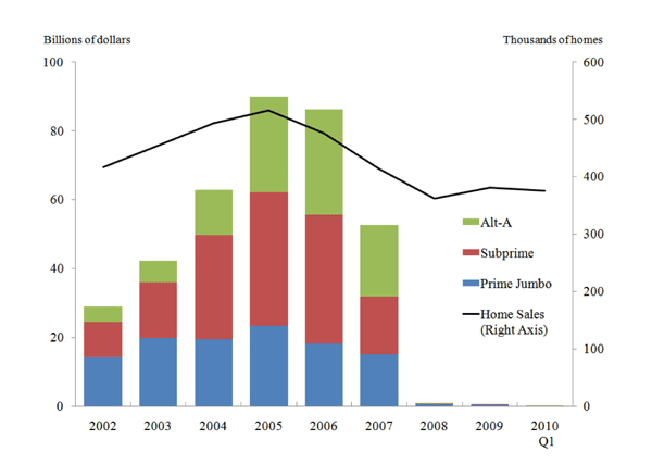
Source: Inside Mortgage Finance and National Association of Realtors.

Data for Figure 1

Year	Prime Jumbo (billions of dollars)	Subprime (billions of dollars)	Alt-A (billions of dollars)	Home Sales (thousands of homes)
2002	14.29453333	10.22340833	4.455233333	416.3652968
2003	19.787875	16.24654167	6.17925	453.739726
2004	19.448175	30.21245	13.215475	492.8984517
2005	23.39196667	38.75301667	27.6936	515.1255708
2006	18.25311667	37.3833	30.47298333	475.8287671
2007	15.03853333	16.79556667	20.80083333	412.913242
2008	0.554825	0.18845	0.154558333	361.4708561
2009	0.459741667	0.072866667	0	380.609589
2010	0	0	0.238966667	375.1018519

Figure 2. Global CDO Issuance, Annual Rate

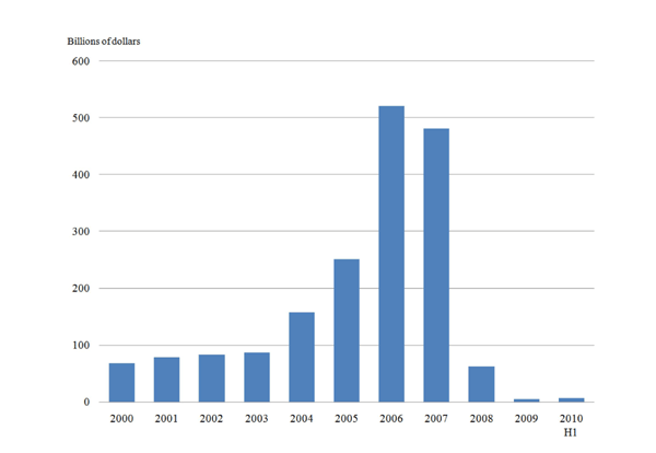
Source: Securities Industry and Financial Markets Association (SIFMA).

Data for Figure 2

Year	Total (billions of dollars)
2000	67.9877
2001	78.4538
2002	83.0743
2003	86.6298
2004	157.8207
2005	251.2653
2006	520.6446
2007	481.6007
2008	61.8868
2009	4.336
2010-H1	6.3744

Figure 3. Trading When Securities are Uniformly Distributed Between L=60 and U=130

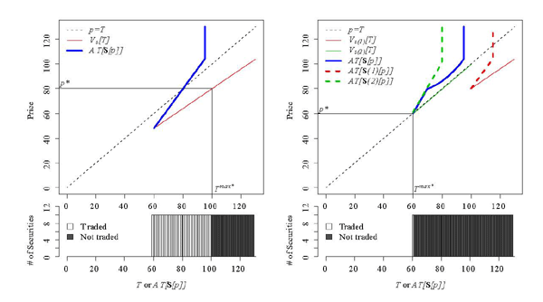
Left panel: Seller's discount (x) is set to 0.8, and only some securities will trade.
Right panel: Second round of trading.

Figure 4. Trading When Securities are Uniformly Distributed Between L=0 and U=130

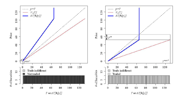
Left panel: Seller's discount (x) is set to 0.8, and only securities with T=0 will trade.
Right panel: x=0.4 and all securities trade.

Figure 5. Left Panel: A significant mass of payoffs close to zero can preclude all trade. Right Panel: Multiple equilibria.

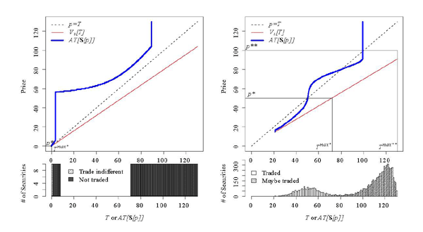
Figure 6. Trading with the Possibility of Appraisal

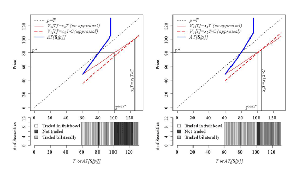
Left panel: Appraisal cost is 25.
Right panel: Appraisal cost is 21.

Figure 7. Priors for π

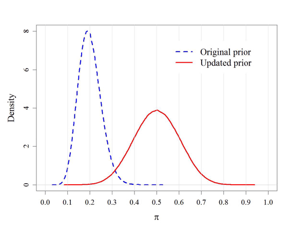
Figure 8. Securitization of Mortagages

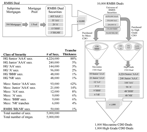
Figure 9. Left Panel: Density of mortgage types. Right Panel: Mapping from mortgage types to mortgage payoffs.

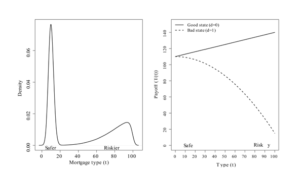
Figure 10. Expected Payoffs of Mortgage Pools When π=0.5

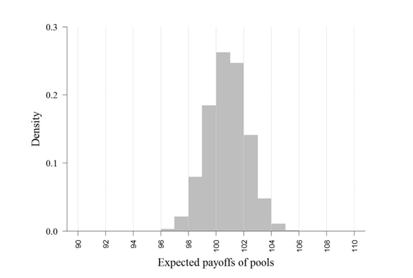
Figure 11. Left Panel: Density of mortgage payoffs. Right Panel: Cumulative density of mortgage payoffs.

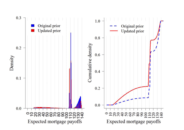
Figure 12. Payoffs of Mortgage Pools and RMBS Securities Under Original Prior (Blue) and Updated Prior (Red)

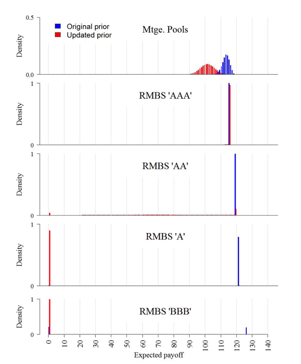
Figure 13. Payoffs of High Grade CDO Securities Under Original Prior (Blue) and Updated Prior (Red)

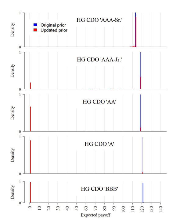
Figure 14. Payoffs of Mezzanine CDO Securities Under Original Prior (Blue) and Updated Prior (Red)

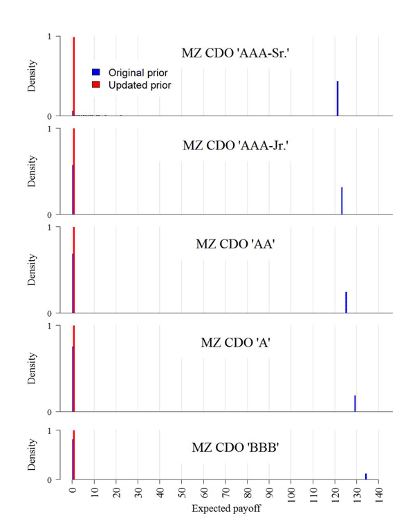
Figure 15. Trading of High Grade (CDO) Securities Under Asymmetric Information

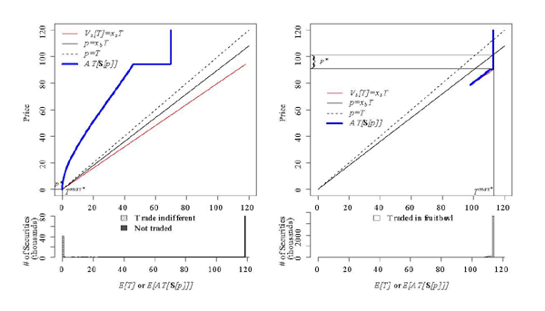
Left panel: Market for High Grade 'AAA-Junior' CDOs when x_s=0.8 and x_b=0.9.
Right panel: Market for High Grade 'AAA-senior' CDOs.

Figure 16. Knife-Edge Equilibria When CDOs Rated 'A' and Higher are Grouped Together

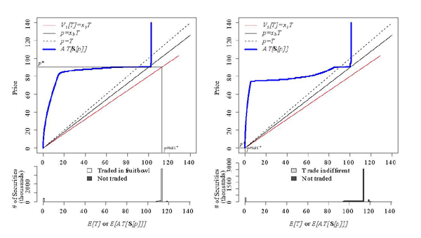
Left Panel: Updated prior (almost everything trades).
Right Panel: Uniform prior (nothing trades).

Figure 17. TARP Program

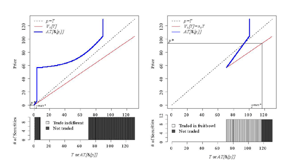
Left Panel: Pre-TARP Equilibrium.
Right Panel: Post-TARP Equilibrium.

Figure 18. Bad Bank

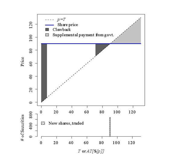
Footnotes

1.  The authors are economists in the International Finance Division of the Federal Reserve Board. We are indebted to Gene Phillips, John Ammer, Neil Ericsson, and participants of the 2010 International Risk Management Conference in Florence, Italy, for their helpful comments. We also thank Ronel Elul for a thoughtful discussion of our paper at the Global Financial Crisis research workshop held at the Federal Reserve Board. Finally, we benefited from the excellent research assistant by Grant Long and Zachary Kurtz. The views in this paper are solely the responsibility of the authors and should not be interpreted as reflecting the views of the Board of Governors of the Federal Reserve System or of any other person associated with the Federal Reserve System. Return to text

2.  Throughout this paper, the term "asset-backed securities" is used in the broad sense and encompasses residential mortgage backed securities (RMBS) and collateralized debt obligations (CDOs). Return to text

3.  The U.S. Treasury acknowledged this in a White Paper accompanying the March 23, 2009 press release announcing the details of the Public-Private Investment Program to purchase troubled assets. The White Paper states that "while fundamentals have surely deteriorated over the past 18-24 months, there is evidence that current prices for some legacy assets embed substantial liquidity discounts."(U.S. Department of Treasury (2009)) Return to text

4.  We broaden the definition of "the sell-side" to include both issuers (those that produced the securities) and people who have previously purchased the securities and have held them for long enough to know what they are really worth. Return to text

5.  Although our analysis focusses on the CDO market, the conclusions would readily apply to the market for asset-backed commercial paper (ABCP). Similar to CDOs, information about the underlying loans backing ABCP was lost along the chain. Return to text

6.  This securitization scheme is based on the example in Gorton (2007). Return to text

7.  In yet another level of securitization which we ignore here, CDO and RMBS tranches may be purchased by other CDOs ("CDO-squareds") or asset-backed commercial paper conduits. Return to text

8.  The model is stylized because we ignore issues like the timing and intensity of defaults and prepayments, and also the complex covenants and triggers present in RMBS and CDO deals. Return to text

9.  The underlying distribution of mortgage types is a combination of two beta distributions. The "safe" mortgage types are characterized by a beta distribution with mean 10 and standard deviation of 2. The "risky" mortgage types are drawn from a beta distribution with mean 80 and standard deviation of 15.  Return to text

10.  The density of the payoffs of the residual RMBS and CDO tranches (not shown) exhibit expected returns which are very high and dispersed under the original prior. Their expected returns fall to zero when the prior is updated. Return to text

11.  Often, but not always, CDO issuers acknowledge the potential for conflicts of interest in their prospectuses. For example, the prospectus of a CDO registration with the Securities and Exchange Commission by Everquest Financial Ltd. contains four full pages detailing the various types of conflicts of interest that may arise. The prospectus states that material losses could occur because of "the existence of conflicts of interests in our relationship with BSAM and/or its affiliates and with Stone Tower and/or its affiliates, which could result in decisions that are not in the best interests of our shareholders." (EDGAR Online, Inc. (2007)). Return to text

12.  Source: BlackRock Solutions as of May 7, 2010. Return to text

13.  The Congressional Oversight Panel recognized the enormous amount of uncertainty surrounding their estimate: "It is impossible to ever arrive at an exact dollar amount of troubled assets, but even the challenges of making a reliable estimate are formidable." (Congressional Oversight Panel (2009a))  Return to text

14.  The government is also slightly better off because it was fully reimbursed for the lemons it acquired, but these lemons are still worth something.  Return to text

15.  This approach was adopted in Germany. For an analysis of the German Bad Bank proposal see Lehment (2009). Return to text

This version is optimized for use by screen readers. Descriptions for all mathematical expressions are provided in LaTex format. A printable pdf version is available. Return to text

Home | Economic research and data | Publications and education resources
Accessibility | Contact us
Last update: October 27, 2010