Skip to: [Printable Version (PDF)]

Board of Governors of the Federal Reserve System
International Finance Discussion Papers
Number 977, May 2010 --- Screen Reader Version*

News and Sovereign Default Risk in Small Open Economies^**

Ceyhun Bora Durdu, Ricardo Nunes, and Horacio Sapriza

NOTE: International Finance Discussion Papers are preliminary materials circulated to stimulate discussion and critical comment. References in publications to International Finance Discussion Papers (other than an acknowledgment that the writer has had access to unpublished material) should be cleared with the author or authors. Recent IFDPs are available on the Web at http://www.federalreserve.gov/pubs/ifdp/. This paper can be downloaded without charge from the Social Science Research Network electronic library at http://www.ssrn.com/.

Abstract:

This paper builds a model of sovereign debt in which default risk, interest rates, and debt depend not only on current fundamentals but also on news about future fundamentals. News shocks affect equilibrium outcomes because they contain information about the future ability of the government to repay its debt. First, in the model with news shocks not all defaults occur in bad times, bringing the model closer to the data. Second, the news shocks help account for key differences between emerging markets and developed economies: as the precision of the news improves the model predicts lower variability of consumption, less countercyclical trade balance and interest rate spreads, as well as a higher level of debt more in line with the characteristics of developed economies. Finally, the model also captures the hump-shaped relationship between default rates and the precision of news obtained from the data.

Keywords: Sovereign default risk, news shocks, endogenous borrowing constraints

JEL classification: F34, F41

1  Introduction

News about future fundamentals can be a significant driving force of economic fluctuations, since they can affect agents' expectations and influence their current decisions.¹ One key source of country heterogeneity lies precisely in the ability to extract news regarding future economic developments that are relevant for forecasting and current decision making. A second relevant difference across countries relates to sovereign default risk and interest rate spreads, which can be a significant factor determining the dynamics of macroeconomic variables in small open economies.

While news and default risk have been examined separately, there is very little work exploring the implications of their joint dynamics. By affecting the incentives to default, news changes the economy through the effects on interest rate spreads. These forces were visibly at play in the 2010 debt crisis affecting some countries in the European Union. On February 3rd 2010, for instance, the Commissioner for Economic and Monetary Affairs Joaquín Almunia stated that besides Greece, Portugal and Spain were facing a loss in productivity - "For instance, those countries [Portugal and Spain] are facing a permanent loss in productivity ...". These remarks were interpreted as news in which European Union experts deemed likely that future economic conditions would continue to be relatively unfavorable in these countries. As shown in Figure 1, Credit Default Swaps increased immediately after Almunia's remarks.

Figure 1. Five-year CDS Spread

Notes: The graph on the left shows the 5-year CDS spreads for Spain (solid line) and Portugal (dashed line). The vertical line points to February 3. The graph on the right reflects a more focused version than the one on the left.

Our paper analyzes the extent to which changes in expectations -due to policy announcement or news in general- matter for macroeconomic fluctuations across countries. To pursue our goal, we build a quantitative dynamic small open economy model of sovereign debt and default subject to both contemporaneous and news shocks. Every period, the economy receives a stochastic endowment, as well as a noisy signal about next period's endowment. Households value private consumption and the government borrows from abroad to smooth consumption. Foreign lenders charge a risk premium that accounts for the default risk they face, so interest rate spreads reflect the time varying sovereign default risk. We examine the model implications quantitatively using direct data. Hence, we show the plausibility of our findings not only from a theoretical point but also from a quantitative perspective. In the quantitative analysis, we calibrate the model without news to a typical emerging market economy following Arellano (2008) and then we explore how news about future output affects the predictions of the model.

Our quantitative analysis delivers three key findings. First, we find that introducing news can account for the empirical fact that not all defaults occur in bad times. We find that negative news can lead to a default, even if current output is high. Negative news regarding future fundamentals increase next period's default risk, which immediately raises the interest rate paid by the sovereign. As the sovereign faces tighter conditions to roll-over debt, she may default in the current period. This mechanism highlights the interaction between news and default risk. Besides having direct effects, news may significantly affect default risk, which in turn, alters the fluctuations of several key macro aggregates.

Second, we find that the differences in the precision of news on future fundamentals helps rationalize differences in the fluctuations of several macroeconomic variables between emerging and industrialized economies.² The model economy where there is no news largely captures the dynamics of macroeconomic variables in emerging markets. As news becomes more informative, the model statistics get closer to those for developed countries. Our first set of findings is consistent with the premise that while agents in industrialized countries can generally rely on information systems that provide relatively accurate news, information is scarcer or less precise in most middle and low income countries.³

Finally, the model predicts a hump-shaped relationship between default rates and precision of news. More precise news enable agents to better manage the debt instrument used to smooth consumption, which lowers the country's default rate for any given amount of debt. At the same time, the lower risk profile allows the economy to sustain more debt in equilibrium which leads to more defaults. This theoretical prediction is confirmed by the data. In particular, the finding is in line with the empirical regularity about how income per capita levels are related to the historical default rates. Using data for 163 countries covering the 1950-2003 period, we document a hump-shaped relationship between per capita income levels and default rates.

Our paper is related to several strands of the literature. First, we borrow from the news and learning literature. Pigou (1927) is among the first to consider that shifts in expectations about future fundamentals are important sources of macroeconomic fluctuations. More recently, Cochrane (1994) and Beaudry and Portier (2004) find that news about total factor productivity or stock prices can explain a significant portion of the forecast variance of consumption, output and hours. Building on the real business cycle literature, Jaimovich and Rebelo (2008) and Schmitt-Grohe and Uribe (2008) explore the importance of news using log-linear approximation methods. Differently from these papers, we focus on how news shocks interact with default risk in a dynamic stochastic quantitative model of endogenous sovereign debt and default. In addition, unlike those studies, we employ nonlinear approximation methods, which is crucial to capture changes in precautionary savings due to differences in news precision.

Boz et al. (2009) build on the work of Aguiar and Gopinath (2007) with trend growth and transitory shocks. When the model economy is subject to greater uncertainty regarding the decomposition of total factor productivity to its trend growth and transitory components, the economy displays characteristics that are more similar to emerging market countries. Related to this literature, Fernández-Villaverde et al. (2009) emphasize the role of uncertainty regarding interest rate fluctuations in driving the behavior of macroeconomic aggregates in emerging economies. Complementing these studies, our framework explores how news about future fundamentals affects sovereign default risk and macroeconomic fluctuations.

Second, our paper is related to the recent literature on quantitative models of sovereign debt. Following the seminal work of Eaton and Gersowitz (1981), various studies have focused on how default risk affects economic fluctuations. A short list of papers includes Chatterjee et al. (2007), who study unsecured consumer default; Aguiar and Gopinath (2006), Arellano (2008), Cuadra and Sapriza (2008), Hatchondo, Martinez and Sapriza (2009), Lizarazo (2006), Mendoza and Yue (2008), Yue (2010), among others, who analyze various features of the dynamics of sovereign debt and default in emerging markets. Our paper advances on this literature by looking at the implications of news shocks on the behavior of sovereign spreads and international debt flows to small open economies.⁴ To our knowledge, our paper presents the first effort to integrate news and default risk in a nonlinear dynamic stochastic quantitative model of endogenous default.

Tomz and Wright (2007) document that a significant fraction of defaults have occurred in good times. The previously cited models can not easily account for this empirical evidence. The only paper that accounts for this regularity is Hatchondo, Martinez and Sapriza (2009). Hatchondo et al. (2009) build a model with political uncertainty and characterize the equilibrium dynamics under which default can occur in good times. Unlike their study, our model does not resort to political distortions that can be difficult to measure.

As we highlighted earlier, our model helps to explain cross country heterogeneity based on the improvement in the precision of news through its effect on endogenous credit risk dynamics. The probability of default and the associated risk premium in an incomplete markets setting are the major factors in explaining the business cycle fluctuations in these economies. Empirical studies have estimated these probabilities and have found that incentives to default are higher in recessions.⁵ The countercyclicality of interest rate spreads in the model is closely linked to the dynamics of the default probabilities perceived by the market. This is consistent with the empirical evidence documented in Neumeyer and Perri (2005) and Uribe and Yue (2006). These studies show that the cost of foreign credit is higher in recessions than in expansions. Similarly, Cantor and Packer (1996) find that sovereign credit ratings strongly respond to the GDP growth rate.

The rest of the paper is organized as follows. Section 2 presents the economic environment and the theoretical framework. Section 3 analyzes the quantitative implications of the benchmark model and Section 4 concludes.

2   The Model

We consider a small open economy model with households, government and foreign lenders. We first describe the stochastic structure and the news shocks.

2.1   Stochastic Structure and News Shocks

The endowment is assumed to follow an AR(1) process

$$\ln(y_{t})=\rho\ln(y_{t-1})+\varepsilon_{t},$$ (1)

with $E\left( \varepsilon\right) =0$ and $E\left( \varepsilon^{2}\right) =\sigma_{\varepsilon}^{2}$. The process is approximated using a discrete one-period Markov chain with probabilities $p(y_{t+1}=m\vert y_{t}=j)$ $\forall m,j\in\Theta$, where $\Theta$ denotes the probability space for the endowment. We consider that in any period the government receives a signal ($s$) regarding next period's endowment. Due to the signal's predictive content, it will lead the government to revise its forecast. Conditional on a future endowment ($y_{t+1}$) we need to specify the probability of receiving a given signal ($s_{t}$) in the current period. In other words, we need to define $p(s_{t}=i\vert y_{t+1}=l)$, with $l\in\Theta$ and $i\in\Xi$, where $\Xi$ denotes the probability space for the signal.

The sets $\Theta$ and $\Xi$ do not necessarily coincide. One may consider the case where the government only receives signals regarding some future endowments, in which case $\vert\Theta\vert>\vert\Xi\vert$. One can also consider the opposite case with $\vert\Theta\vert<\vert\Xi\vert$. This corresponds to the case in which, for instance, there are signals corresponding to each element in $\Theta$, and in addition there are signals corresponding to joint elements of $\Theta$. In the current paper, we consider $\vert\Theta\vert=\vert\Xi\vert$ and that for each element in $\Theta$ there exists one and only one element in $\Xi$.

The signal ($s_{t}$) is then incorporated into the forecast of next period's endowment ($y_{t+1}$). Following Bayes' theorem, the forecast conditional on current information is given by:

$$p(y_{t+1}=l\mid s_{t}=i,y_{t}=j)=\frac{p(s_{t}=i\mid y_{t+1}=l)p(y_{t+1}=l\mid y_{t}=j)}{\underset{n}{\sum}p(s=i\mid y_{t+1}=n)p(y_{t+1}=n\mid y_{t} =j)}$$ (2)

with $l,j,n\in\Theta$ and $i\in\Xi$. For the quantitative analysis, it is convenient to express the Markov chain for the joint evolution of the endowment shock and the signal. This can be implemented with the following formula:

$$\Pi(y^{\prime},s^{\prime},y,s)=p(s_{t+1}=\kappa,y_{t+1}=l\vert s_{t}=i,y_{t}=j)= p(y_{t+1}=l\vert s_{t}=i,y_{t}=j)$$

$$\sum_{m}\left[ p(y_{t+2}=m\vert y_{t+1}=l)p(s_{t+1}=\kappa\vert y_{t+2}=m)\right]$$ (3)

with $l,j,m,l\in\Theta$ and $i,\kappa\in\Xi$. Regarding the signal precision, we examined different parameterizations and formulations. We first assumed that

$$p(s_{t}=i\vert y_{t+1}=l)=\left\{ \begin{array}[c]{c} \eta\text{ \ \ \ \ \ \ \ \ \ \ \ \ \ \ \ \ \ \ \ \ if }i=l\\ (1-\eta)/(\vert\Xi\vert-1)\text{ if }i\neq l \end{array} \right. .$$ (4)

When $\eta=1/\vert\Xi\vert$ the signals are not informative, and when $\eta=1$ the government can perfectly anticipate the endowment shock one period ahead. In the quantitative analysis, we explore several cases with $1/\vert\Xi\vert\leq\eta \leq1$.⁶

We also assume that the signal is public information, i.e., the government, private agents and external lenders all observe the same signal and adjust their actions accordingly. A model where some agents receive more precise signals is interesting, but raises issues of asymmetric information that are beyond the scope of this paper.

2.2   Households

The representative household is a hand-to-mouth consumer with preferences given by the present value of the sum of instantaneous utility functions:

$$E_{0}\sum_{t=0}^{\infty}\beta^{t}u(c_{t})$$ (5)

The per period utility is concave, strictly increasing and twice differentiable. The discount factor is $\beta\in(0,1)$ and households derive utility from private consumption $c_{t}.$ In the numerical work, we use a CRRA per period utility function $u(c) =c^{(1-\sigma)}/(1-\sigma)$.

2.3   Government

The benevolent government maximizes the utility of the households. Financial markets are incomplete since the government can only save and borrow using a non-contingent, one-period bond traded in international capital markets.⁷ Each period, conditional on being in good credit standing, the government chooses between honoring its outstanding foreign debt or defaulting on it. This decision comes from comparing the net benefits of the two options. The government compares the cost of temporary exclusion from credit markets given by the foregone benefits of consumption smoothing and the output loss in autarky, against the direct costs of repayment given by the short-run disutility of lowering current consumption to repay the non-contingent loan.

Every period, given the underlying state of nature, the signal on next period's income and the amount of outstanding foreign assets, the government chooses whether to repay the current debt or default. If it chooses to repay, it continues to have access to the capital markets, and decides how much to borrow or save. To be more precise, the state variables are the realization for income ($y$), the realization for the signal ($s$), the level of foreign assets ($B$) and the credit situation of the country ($D$), where $D=1$ if the economy has access to credit markets and 0 if the economy is in financial autarky.

The government optimization problem can be expressed in a recursive dynamic programming form. The value function when the government has access to international markets and begins the period with an amount of assets $B$ and shocks ($y,s)$ is given by $V_{0}(B,y,s)$. The value associated with paying back and remaining in the credit market is given by $V^{c}(B,y,s)$, whereas the value associated with defaulting and switching to temporary autarky is given by $V^{d}(y,s)$. The problem can be expressed in the following way:

$$V_{0}(B,y,s)=\max\left\{ V^{c}(B,y,s),V^{d}(y,s)\right\}$$ (6)

and the optimal default decision of the government is characterized by

$$D(B,y,s)=\left\{ \begin{array}[c]{c} ~\ \ 1\text{ \ \ \ \ \ \ \ \ \ \ \ \ \ \ }if\text{ \ }V^{c}(B,y,s)>V^{d} (y,s)\text{ \ }\\ 0\text{ \ \ \ \ \ \ \ \ \ \ \ \ \ \ \ \ \ } otherwise\text{\ \ \ \ \ \ \ \ \ \ \ \ \ \ \ \ \ } \end{array} \right. .$$ (7)

The default policies determine a repayment set $\Gamma(B)$ defined as the set of values of the productivity and the news shock such that repayment is optimal given the level of foreign assets $B$,

$$\Gamma(B)=\{(y,s)\in \Upsilon:D(B,y,s)=1\}.$$ (8)

The default set $\digamma(B)$ defined as the set of values of the productivity and news shocks such that default is optimal given asset holding level $B$,

$$\digamma(B)=\{(y,s)\in \Upsilon:D(B,y,s)=0\}.$$ (9)

If the government does not default, the economy can issue new debt and finance consumption subject to the following resource constraint:

$$c=y+B-q(B^{\prime},y,s)B^{\prime},$$ (10)

where $q(B^{\prime},y,s)$ is the price of the bond. When the sovereign borrows, it receives $q(B^{\prime},y,s)B^{\prime}$ units of consumption goods from foreign creditors on the current period and promises to pay $B^{\prime}$ units next period conditional on not defaulting. Hence, the bond price reflects the probability of default, which depends on $B^{\prime},y$ and $s$.⁸ Then the government maximization problem can be formulated as follows:

$$\begin{split}V^{c}(B,y,s) & =\max_{B^{\prime}}\left\{ U(y+B-q(B^{\prime},y,s)B^{\prime })+\beta\sum_{y^{\prime},s^{\prime}}V_{0}(B^{\prime},y^{\prime},s^{\prime} )\Pi(y^{\prime},s^{\prime},y,s)\right\} \\ \text{s.t.} \quad c & =y+B-q(B^{\prime},y,s)B^{\prime}. \end{split}$$ (11)

When the government defaults on its debt the country is temporarily excluded from international credit markets. In addition, following Arellano (2008), the economy suffers an output loss that lowers income to $y^{def},~$ so that consumption $c^{d}=y^{def}$.⁹ More specifically we assume the following specification

$$y^{def}=\left\{ \begin{array}[c]{c} \phi E\left( y\right) \quad\text{if}\quad y>\phi E\left( y\right) \text{ \ }\\ y \quad\text{\ \ \ \ \ if} \quad y\leq\phi E\left( y\right) \end{array} \right. ,$$ (12)

with $\phi\in(0,1)$. The value function under default is given by:

$$V^{d}(y,s)=U(y^{def})+\beta\sum_{y^{\prime},s^{,\prime}}\left[ \mu V_{0}(0,y^{\prime},s^{\prime})+(1-\mu)V^{d}(y^{\prime},s^{\prime})\right] \Pi(y^{\prime},s^{\prime},y,s).$$ (13)

While in autarky, the country may regain access to external markets with an exogenous probability $\mu$. When the economy returns to financial markets, it does so with no debt burden, $B=0$, and with a continuation value $V_{0}(0,y,s)$. Conversely, the country may stay in autarky with a probability $1-\mu\$, and the continuation value $V^{d}\left( y,s\right)$.

2.4   Foreign Lenders

There is a large number of identical, infinitely-lived foreign creditors. Each lender can borrow or lend at the risk free rate $r_{f}$ and participates in a perfectly competitive market to lend to the small open economy. Lenders are risk-neutral and maximize expected profits as follows:

$$\Phi=-qB^{\prime}+\frac{\lambda(B^{\prime},y,s)}{1+r_{f}}0+\frac {(1-\lambda(B^{\prime},y,s))}{1+r_{f}}B^{\prime}.$$

The first term in the equation above shows that when creditors lend to the government in the current period, they buy the discount bond issued by the domestic government at a price $q$. Next period, the lenders may receive the face value of the bond depending on whether the government defaults or not. When it defaults, creditors get 0 units of the consumption good, where $\lambda(B^{\prime},y,s)$ is the endogenous probability that the government defaults on its sovereign debt. The probability of default $\lambda(B^{\prime },y,s)$ is endogenously determined as

$$\lambda(B^{\prime},y,s)=\sum_{y^{\prime},s^{\prime}\in \digamma(B^{\prime})}\Pi(y^{\prime},s^{\prime},y,s),$$ (14)

so that the default probability is zero when $\digamma(B^{\prime} )=\varnothing$ and it is one when $\digamma(B^{\prime})=\Upsilon.$

Since there is perfect competition in the credit market, a zero profit condition holds for the foreign creditors.¹⁰ The bond price is then

$$q(B^{\prime},y,s)=\frac{(1-\lambda(B^{\prime},y,s))}{1+r_{f}}.$$ (15)

2.5   Equilibrium Definition

A recursive equilibrium for this small open economy is characterized by a set of value functions for the government, $V_{0},V^{c},V^{d}$; a set of policy functions for household's consumption $c$, $c^{d}$; policy functions for government's default decision $D$; optimal asset holdings $B^{\prime}$; and a bond price function $q$ such that

1. Given the government policies and the bond price function, the household policies for consumption solve the household's problem,
2. Given the bond price function $q$ and the optimal policies for households, the government's value functions $V_{0},$ $V^{c}$ and $V^{d}$ and its policy functions $D$ and $B^{\prime}\$ solve (6), (11) and (13),
3. The equilibrium bond price $q(B^{\prime},y,s)$ is such that zero expected profit condition for foreign creditors holds as described in equation (15).

2.6   First Order Conditions from the Government's Problem

The Euler equation for the government is obtained from the first order condition of its dynamic optimization problem and the envelope theorem:

$$u_{c}\left( c\right) \left[ q+B^{\prime}\frac{\partial q}{\partial B^{\prime}}\right] =\beta\sum_{(y^{\prime},s^{\prime})\in \Gamma(B)}u_{c}\left( c^{\prime}\right) \Pi(y^{\prime},s^{\prime},y,s).$$ (16)

For each unit of additional borrowing, the government increases the current level of consumption by $q+B^{\prime}\frac{\partial q}{\partial B^{\prime}}$ units. The term $B^{\prime}\frac{\partial q}{\partial B^{\prime}}$ reflects that when evaluating the benefits and costs of additional external borrowing, the government takes into account that issuing more bonds decreases their price. The decreasing bond price implies that the government does not obtain as many resources from selling bonds as it would under a constant bond price. The right hand side of equation (16) computes the borrowing costs. Next period, the government should repay its debt, which reduces future consumption. However, consumption only falls in those states in which the government does not default.

3   Quantitative Analysis

The calibration is based on existing work by Arellano (2008) and is set to mimic empirical regularities of emerging markets. The parameters of the model are displayed in Table 1. Table 2 shows business cycle moments of key macroeconomic variables from the data.¹¹ We now turn to the simulation results and the statistical properties of the model. Table 3 displays a set of moments from the simulated model. The statistics reported are average values of 500 simulations with 2001 periods each. The simulated series are logged and filtered.

Table 1. Calibration

Parameter	Notation	Value
Risk Aversion	σ	2
Discount Factor	Β	0.953
Reentry Probability	μ	0.282
Default Pentalty	φ	0.969
Risk Free Interest Rate	rf	0.017
Autocorrelation of Output	ρ	0.945
Standard deviation of output	σε	0.025
News shock	η	[0,0.99]

Table 2. Business Cycle Moments in the Data

	Emerging Markets	Developed Economies
σ(c)/σ(y)	1.45	0.94
ρ(y,c)	0.72	0.66
ρ(y,tb/y)	-0.51	-0.17
ρ(y,Spread)	-0.55	0.20

3.1  No News Case

The model economy without news is identical to the models of sovereign default analyzed in the literature (e.g., Arellano (2008), among others).¹² The no news economy experiences procyclical borrowing induced by changes in default incentives. The availability of external credit and the interest rate vary with the business cycle: foreign lenders respond to an improvement in the domestic macroeconomic conditions by demanding a lower risk premium, which leads the government to borrow.¹⁴ Therefore, when debt carries default risk, the economy borrows more in booms than in recessions. This translates into countercyclical interest rates and trade balance. In addition, the variability of consumption is close to ten percent higher than the variability of output (Table 3).

3.2  Effects of News

Figure 2 plots the discount bond price schedule as a function of assets for two values of the news shock and a given output realization.¹⁴ For all levels of debt, the bond price is lower when the economy is hit by an adverse news shock. Since adverse news shocks about future productivity reveal information about potential difficulties of the government to repay its debt, risk-neutral lenders charge a higher risk premium on impact.

Table 3. Simulation Results

	No News	With News, η=0.9
σ(c)/σ(y)	1.10	1.03
ρ(y,c)	0.97	0.89
ρ(y,tb/y)	-0.23	0.17
ρ(y,Spread)	-0.28	-0.13

Figure 2. News and Bond Price Schedule

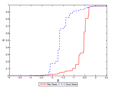
Notes: In the plot, η = 0.5 and the current endowment is at steady-state. The good and bad news cases refers to a signal of an increase and a decrease of 2.3% in the endowment, respectively.

Figure 3 shows the borrowing policy function as a function of and given for two values of the news shock. Good news reduces default risk and lowers the cost of debt, inducing further borrowing. In addition, good news implies that current output is lower than tomorrow's, which leads the government to borrow through an intertemporal substitution mechanism.

News shocks can affect the decision to default. Figure 4 illustrates the shape of the default region as a function of current debt and news shock realizations for the mean output level. The figure displays an S-shaped pattern. Signals () near the current endowment level impact the default decision, while extreme signals do not. The reason for this observation lies in the structure of the shocks. Given the Markov chain representation of the stochastic process for output, it is very unlikely to observe sudden changes in the endowment from one period to another. As shown in Equation (2), the updated probability to observe an endowment next period depends on both the signal and on the Markov chain. If an extreme signal is observed, it is effectively discounted and is interpreted as uninformative news. Conversely, plausible positive and negative signals do affect decision rules.¹⁵ As we will explain later, the S-shaped default region also implies that if the news signal is sufficiently negative and informative, the economy can experience default episodes even when the current output realizations are above their trend value.

Figure 3. News and Savings Policy

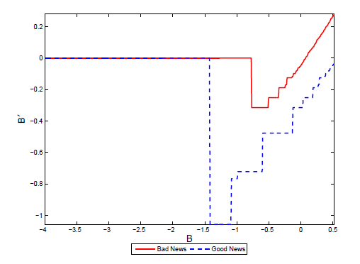
Notes: See notes for figure 2.

Figure 4. News and Default Region

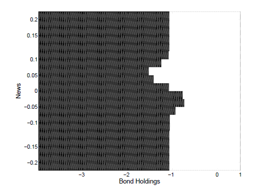
Notes: In the plot, η = 0.5 and the current endowment is at steady-state. The dark region indicates
default.

3.3   News Precision in Emerging and Developed Economies

Emerging markets are distinct from developing countries along several dimensions at the business cycle frequency. Table 2 shows some of the key differences identified in the literature: emerging markets are characterized by a higher variability of consumption relative to output, a higher correlation of consumption with output, a higher and countercyclical interest rate spreads and a countercyclical current account. In addition, developed economies have better information systems and are more closely monitored than emerging markets. News shocks help to explain these stylized facts by considering different levels of precision of news about future income realizations. When news shocks are more precise, the economy can anticipate future fundamentals more accurately and consumption smoothing becomes more effective, reducing the volatility of consumption relative to the volatility of output. In addition, bond prices respond to news in addition to output shocks, dampening the correlations of consumption, trade balance and spreads with current output. As Table 3 illustrates, when η is increased to 0.9, all moments move closer to those characterized by developed economies. Consistently, Figure 5 shows that as the news precision increases in the model, the variability of consumption relative to output and the correlation of trade balance with output get closer to those of developed economies.

3.4   Default in Good Times

The presence of news shocks is also able to rationalize the finding in the literature that a fraction of defaults occur when output is above trend. In particular, Tomz and Wright (2007) find that countries do not always default in bad states of nature. Figure 6 shows that a significant fraction of defaults have occurred when income was above trend for a large set of countries during the period from 1950 to 2003. Moreover, the figure also uncovers a new feature of the data: the fraction of the defaults that occurred in good times becomes higher for countries with higher income per capita levels. The quantitative results depicted in Figure 7 show that our model helps rationalize both stylized facts. Bad news can lead to an immediate default because it predicts that future output will be lower, which will make current debt repayments more costly. Hence, bond prices fall, leading to a deterioration in the current financing decisions and bringing forward the default decision. This mechanism can lead the economy to default even though the current state of the economy is positive. If news are more informative, this mechanism is obviously stronger. Our paper complements Hatchondo, Martinez and Sapriza (2009), which provide an explanation for the observation that countries default in good times by focusing on borrowers' heterogeneity (political risk). Unlike their study, our model does not resort to political distortions that can be difficult to measure. Moreover, our model also helps to explain the higher fraction of defaults in good times observed for the higher income per capita economies.

Figure 5. The Effect of Precision of News on Macroeconomic Variables

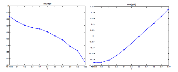
Notes: The graph on the left shows the variability of consumption relative to output, the graph on the right shows the correlation of trade balance with output as a function of the news precision, η.

 

3.5   News Precision, Hump-Shaped Default Pattern

When the economy receives more precise news, forecasts become more accurate and debt management more efficient. Since the signals are public information, international lenders can better assess beforehand the likelihood of default and lend more debt in equilibrium.¹⁶ In addition, the lower risk profile reduces the demand for precautionary savings which induces the economy to increase borrowing. The left panel of Figure 8 plots the debt level as a function of the news precision. We observe a tendency for more indebtedness as the news precision increases. Such observation is also in line with the data for emerging and developed economies (see for example Mendoza and Oviedo (2006), Durdu et al. (2009)).

Figure 6. Proportion of Defaults in Good Times by Income (1950-2003)

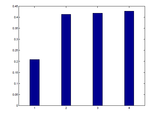
Notes: This figure shows the percentage of defaults that occurred when income was above trend in the data for 118 countries covering 1950-2003 period. Trend income was calculated by fitting a Hodrick- Prescott filter with a smoothing parameter of 100. The bars displayed correspond to different income quintiles. The fifth quintile is not shown, since the only default episode in that group corresponds to Slovenia in 1992, less than a year after its independence and with income below trend.

Figure 7. Percentage of Default in Good Times

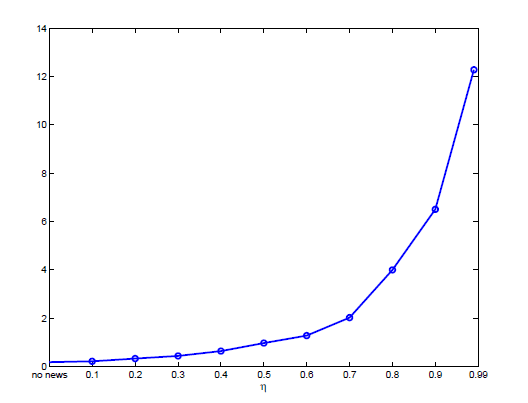
Notes: This figure shows the percentage of defaults occurring in the model when income is above average.

The right panel of Figure 8 shows the default probability as a non-monotonic function of the news precision. This non-monotonicity is at play because of two opposing forces. On the one hand, higher debt levels lead to an increase in the default probability. On the other hand, higher precision leads to better forecasting, making the government more able to avoid costly defaults. The figure shows that for precision levels above 0.6, the latter effect dominates the former. Interestingly, this non-monotonic behavior is consistent with the default rates that we estimate using data for 118 countries covering 1950-2003 (see Figure 9). To the best of our knowledge, our paper is the first to unveil this non-monotonic relation in the data. In addition, we provide a theoretical model that accounts for such feature.

Figure 8. The Effect of News on Debt Dynamics

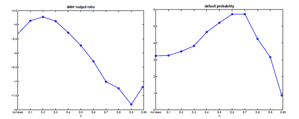
Notes: The graph on the left shows the debt-to-output ratio, and the graph on the right shows the equilibrium default probabilities as a function of the news precision, η.

Figure 9. Default Rates by Income per Capita Brackets: 1950-2003

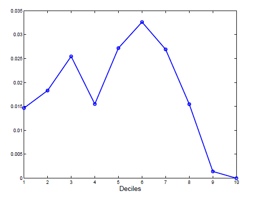
Notes: This figure shows the default rates by income decile that we estimate using data for 118 countries covering 1950-2003.

4  Conclusions

The current crisis has highlighted the importance of news regarding macroeconomic fundamentals, as evidenced by the developments in Greece, Portugal, and Spain among others. In this paper, we build a model of sovereign debt in which default risk, interest rates and debt are affected by current fundamentals and news about future fundamentals. In our framework, news shocks affect equilibrium outcomes because they contain information about the future ability of the government to repay her debt.

In a series of quantitative exercises, we show that news shocks help to account for key differences between emerging markets and developed economies. As the precision of the news improves, the model predicts lower variability of consumption, less countercyclical trade balance and interest rate spreads, as well as a higher level of debt more in line with the characteristics of developed economies. The model also captures the hump-shaped relationship between default rates and the precision of news obtained from the data. In addition, the model with news shocks can generate default episodes in good times, bringing the model closer to the stylized facts established in the literature.

5  Appendix

5.1  Algorithm

We assume an initial function for the price of the bond q₀(B',y,s), as well as initial values for V₀ and V^d. To calculate the initial value of the bond, we use the inverse of the risk free rate. For the initial values of the value functions, (V₀)₀ and (V^d)₀, we start with null matrices. Then we employ the following algorithm:

1. Use to express the per period utility as a function of B, B' , y and s, then use (V₀)₀ and (V^d)₀ and equations (6), (11) and (13) to get (V₀)₁ and (V^d)₁, the policy function, B'(B,y,s) and default function D(B,y,s).

2. Given the default function D(B,y,s), and the repayment and default sets Γ(B) and digamma(B) , compute the probability of default λ(B',y,s) using (14).

3. Update the price of the bond using the following equation: q₁ = (1-λ(B',y,s))/(1+r_f)

4. Use the updated price of the bond q₁ and the value functions (V₀)₁ and (V^d)₁ to repeat steps 1, 2, 3 and 4 until the following conditions are satisfied:

max{q₀(B',y,s)-q₁(B',y,s)} < ε

max{V₀(B',y,s)₀-V₀(B',y,s)₁} < ε

max{V^d(B',y,s)₀-V^d(B',y,s)₁} < ε

where ε is a small number.

5.2  Data

Cross country stylized facts on consumption, net exports are taken from Aguiar and Gopinath (2007), the data on sovereign interest rate correlations with macroeconomic aggregates is obtained from Neumeyer and Perri (2004), the statistics on default rates by income deciles for the period from 1950 to 2003 and the statistics on the proportion of sovereign defaults that occurred above trend by income deciles for the period 1950-2003 (Figure 9) are constructed using the database of sovereign defaults by Beim and Calomiris (2001) and income data from the IMF.

5.3  Alternative Parameterization for the News Signal

In the parameterization for the signal described in Section 2.1, it is more likely to receive a certain signal than any other. For instance, if the endowment (y_t+1) is high there is a corresponding high signal (s_t) that is more likely to be observed. However, conditional on a high endowment (y_t+1), the signals (s_t) corresponding to extremely low or very low endowments are observed with equal probability. We also considered an alternative formulation where it would be more likely to observe signals closer to the endowment:

p(s_t = i|y_t+1 = l) = {η if i = l}{f(i,l) if i ≠ l} where f(i,l) is a function satisfying the property f(i,l) > f(j,l) ↔ |i-l| < |j-l|. In particular, we considered the formula:

p(s_t = i|y_t+1 = l) = η/(e^a|i-l|b_l where a, b_l are positive constants. The precision of the signal is still determined by 1/|Ξ| ≤ η ≤ 1. The results are qualitatively and quantitatively robust across formulations, and for brevity we only report the first set.

Bibliography

Aguiar, M. and G. Gopinath, 2006. Defaultable Debt, Interest Rates and the Current Account, Journal of International Economics 69, 64-83.

Aguiar, M and G. Gopinath 2007. Emerging Markets Business Cycle: The Cycle is the Trend, Journal of Political Economy 115, 69-102.

Arellano, Cristina, 2008. Default Risk and Income Fluctuations in Emerging Economies, American Economic Review 98(3), 690-712.

Beaudry, Paul and F. Portier, 2006. Stock Prices, News, and Economic Fluctuations, American Economic Review 96(4), 1293-1307.

Beaudry, Paul and F. Portier, 2007. When can changes in expectations cause business cycle fluctuations in neo-classical settings?" Journal of Economic Theory, 135(1), 458-477.

Beim, D. and Ch. Calomiris, 2001. Emerging Financial Markets, McGraw Hill.

Boz, E., C. B. Durdu and C. Daude, 2008. Emerging Market Business Cycles Revisited: Learning about the Trend, Federal Reserve Board International Finance Discussion Paper 927.

Cantor, R. and F. Packer, 1996. Determinants and Impact of Sovereign Credit Ratings, Economic Policy Review, Federal Reserve Bank of New York.

Chatterjee, S., D. Corbae, M. Nakajima and V. Rios-Rull, 2007. A Quantitative Theory of Unsecured Consumer Credit with Risk of Default, Econometrica, 75(6), 1525-1589.

Correia, Isabel, Jorge C. Neves and Sergio Rebello, 1995. Business cycles in a small open economy, European Economic Review, vol. 39(6), 1089-1113.

Cuadra G. and H. Sapriza, 2008. Sovereign Default, Interest Rates and Political Uncertainty in Emerging Markets, Journal of International Economics 76, 78-88.

Durdu, C. B., E. G. Mendoza and M. E. Terrones, 2009. Precautionary Demand for Foreign Assets in Sudden Stop Economies: An Assesment of the New Mercantilism, Journal of Development Economics Vol. 89 pp. 194-209, July.

Eaton, J. and M. Gerzovitz,1981. Debt with Potential Repudiation: Theoretical and Empirical Analysis, Review of Economic Studies 48, 289-309.

Fernández-Villaverde, Jesús, Pablo Guerrón-Quintana and Juan F. Rubio-Ramírez, 2009. Risk Matters: The Real Effects of Volatility Shocks, NBER Working Paper 14875.

Hatchondo J., L. Martinez and H. Sapriza, 2008. Heterogeneous Borrowers in Quantitative Models of Sovereign Default, International Economic Review, forthcoming.

Hussey, R., and G. Tauchen, 1991. Quadrature-Based Methods for Obtaining Approximate Solutions to Nonlinear Asset Pricing Models, Econometrica 59, 371-396.

IMF Financial Stability Report, 2007.

Jaimovich, Nir and S. Rebelo, 2009. Can News about the Future Drive the Business Cycle?, American Economic Review, 99(4), 1097-1118.

Lizarazo, Sandra, 2006. Default Risk and Risk Adverse International Investors, Working Paper, ITAM.

Mendoza, Enrique G., 1991. Real Business Cycles in a Small Open Economy, American Economic Review 81, 797-818.

Mendoza, Enrique G. and P. Marcelo Oviedo. Fiscal Policy and Macroeconomic Uncertainty in Developing Countries: The Tale of the Tormented Insurer, NBER Working Paper 12586.

Mendoza, Enrique G. and Vivian Yue, 2008. A Solution to the Default Risk-Business Cycle Disconnect, NBER Working Paper 13861.

Neumeyer, P. and F. Perri, 2005. Business Cycles in Emerging Economies: The Role of Interest Rates, Journal of Monetary Economics 52/2, 345-380.

Schmitt-Grohe, Stephanie and Martin Uribe, 2008. What's News in Business Cycles, Working Paper, Columbia University.

Tomz, Michael, and Mark L. J. Wright. 2007. Do Countries Default in `Bad Times'? Journal of the European Economic Association 5:2-3, 352-360.

Uribe, Martín and Vivian Yue, 2006. Country Spreads and Emerging Countries: Who Drives Whom?, Journal of International Economics 69, 6-36.

Yue, Vivian, 2010. Sovereign Default and debt renegotiation, Journal of International Economics, forthcoming.

Footnotes

**  We are grateful to seminar participants at the Federal Reserve Board for comments. Correspondence: [email protected], [email protected], [email protected]. The views expressed in this paper are solely the responsibility of the authors and should not be interpreted as re�ecting the views of the Board of Governors of the Federal Reserve System or of any other person associated with the Federal Reserve System. Return to text

1.  We use the term "news" to refer to "news shocks." Return to text

2.  As earlier studies show, emerging market economies are more prone to crises, face higher interest rate spreads, and can only sustain lower debt-output ratios than their more developed counterparts. In addition, these economies experience more countercyclical trade balances and sovereign interest rate spreads, making external credit more expensive in bad times. Return to text

3.  News are more precise in higher income per capita countries. In practice, higher income countries are more closely monitored and have more abundant and better quality data. See a formal analysis of this statement in Boz et. al. (2009). Return to text

4.  Mendoza (1991) and Correia, Neves and Rebelo (1995), among others analyze business cycles in small open economies but do not consider default risk. Return to text

5.  See Peter (2002) for a survey of econometric studies on the probability of sovereign default. Return to text

6.  The results are robust to alternative specifications of the news signal, as described in the Appendix. Return to text

7.  Most external debt in developing countries represents government debt. For example, in 1995 during the Mexican financial crisis, sovereign external debt accounted for almost 70% of the total stock of foreign debt in Mexico. Return to text

8.  Notice that there is no commitment problem for the foreign creditors. If the foreign creditors borrow from the domestic government, they always repay their debt. Return to text

9.  The assumption that default reduces output can be rationalized by the fact that default episodes tend to be associated with disruptions in foreign trade and private sector's access to credit, which entail an output loss. See Rose (2005), Arteta and Hale (2006) and Mendoza and Yue (2008). Return to text

10  Alternatively, we could assume that foreign lenders have access to two instruments: a risky bond and a risk free bond. Since creditors are risk neutral, they are willing to buy the risky asset as long as its expected return $R$ equals the return of the risk free asset: $(1-\lambda)(1+R)=1+r_{f}$, with $q=\frac{1}{(1+R)}=\frac {(1-\lambda)}{1+r_{f}}$. Return to text

11.  Data details and sources are described in the Appendix. Return to text

12.  The model without news refers to the case where no signal is observed, or equivalently the signal is observed but has no informational content ( ). Return to text

13.  Additionally, since endowment shocks are persistent, higher future income also induces the government to borrow more. Return to text

14.  The bond price is an increasing function of foreign assets. As shown by earlier studies, for small levels of foreign debt, the government always pays back its debt, so it borrows from international markets at the world risk free interest rate. As foreign debt increases, there is a threshold level for which the bond price starts to decrease reflecting stronger incentives to default for indebted governments. At a sufficiently large debt level the government always defaults regardless of the output realization. At that point the probability of default is one and therefore the bond price is zero. Return to text

15.  For this reason, it is not possible to solve the model with . This calibration would imply transition probabilities that are not well defined for some cases. More specifically, if and , then is not defined. Return to text

16.  Following the literature, the calibration of the discount factor and the risk free rate induces the economy into borrowing. Return to text

This version is optimized for use by screen readers. Descriptions for all mathematical expressions are provided in LaTex format. A printable pdf version is available. Return to text

Home | Economic research and data | Publications and education resources
Accessibility | Contact us
Last update: June 21, 2010