
Board of Governors of the Federal Reserve System
International Finance Discussion Papers
Number 998, June 2010 --- Screen Reader
Version*
Immigration, Remittances and Business Cycles1
NOTE: International Finance Discussion Papers are preliminary materials circulated to stimulate discussion and critical comment. References in publications to International Finance Discussion Papers (other than an acknowledgment that the writer has had access to unpublished material) should be cleared with the author or authors. Recent IFDPs are available on the Web at http://www.federalreserve.gov/pubs/ifdp/. This paper can be downloaded without charge from the Social Science Research Network electronic library at http://www.ssrn.com/.
Abstract:
We use data on border enforcement and macroeconomic indicators from the U.S. and Mexico to estimate a two-country business cycle model of labor migration and remittances. The model matches the cyclical dynamics of labor migration to the U.S. and documents how remittances to Mexico serve an insurance role to smooth consumption across the border. During expansions in the destination economy, immigration increases with the expected stream of future wage gains, but it is dampened by a sunk migration cost that reflects the intensity of border enforcement. During recessions, established migrants are deterred from returning to their country of origin, which places an additional downward pressure on the wage of native unskilled workers. Thus, migration barriers reduce the ability of the stock of immigrant labor to adjust during the cycle, enhancing the volatility of unskilled wages and remittances. We quantify the welfare implications of various immigration policies for the destination economy.
Keywords: Labor migration, sunk emigration cost, skill heterogeneity, international real business cycles, Bayesian estimation
JEL classification: F22, F41
1 Introduction
Labor migration is sizeable and has a significant economic impact on the economies involved. The number of foreign-born residents is rising worldwide: Foreign-born residents made up as much as 13% of the total U.S. population in 2007, compared to less than 6% in 1980, a pattern visible in several other OECD countries (Grogger and Hanson, 2008). Labor migration also varies over the business cycle. Jerome (1926) documented the procyclical pattern of European immigration into the U.S. during the 19th and early 20th centuries, showing that U.S. recessions were associated with drastic declines in immigration flows, while relatively larger inflows occurred during recovery years.4 Adding to this evidence, in Fig. 1 we plot the number of apprehensions at the U.S.-Mexico border (which the existing literature uses as a proxy for attempted illegal crossings into the U.S.) along with the GDP ratio between the U.S. and Mexico measured in purchasing power parity terms; the correlation between the detrended series is 0.44. The chart shows that periods in which the U.S. economy outperformed that of Mexico generally were accompanied by an increase in the number of border apprehensions.5
Immigrant workers send remittances to developing countries on a regular basis. Conservative estimates put the amount of workers' remittances to the developing world at $338 billion in 2008. These totals represent more than 10% of the GDP of several receiving countries,6 while globally they are equivalent to 48% of total private net capital flows to developing economies (including FDI, portfolio equity and private debt).7 Just like labor migration, the remittance flows also vary during the course of the business cycle. Fig. 2 plots the pattern of remittances from the U.S. to Mexico vis-a-vis the relative performance of these economies. Larger outflows of remittances to Mexico occur during periods with faster U.S. economic growth (or lower Mexican growth). The results are even stronger when we compare remittances with the relative wage across the two economies, measured as the ratio between the real wage of unskilled workers in the U.S. (who lack a high school degree) and workers in export assembly plants (maquiladoras) in Mexico; the resulting correlation is 0.79. To sum up, the combined evidence in Fig. 1 and Fig. 2 highlights the potential insurance role of labor migration and remittances to smooth the consumption path for Mexican households whose members reside on both sides of the border.
With this evidence in mind, we examine the business cycle fluctuations of labor migration and remittance flows as well as their propagation to the rest of the economy. We also study the effect of immigration policy (reflected by the magnitude of immigration barriers) on the volatility of migration flows and remittances. To this end, we use a two-country dynamic stochastic general equilibrium (DSGE) model along the lines of Backus et al. (1994), which allows for endogenous labor migration and remittances. To account for skill heterogeneity among the native labor, we introduce two types of labor in the home economy (skilled and unskilled) while assuming that capital and skilled labor are relative complements as in Krusell et al. (2000). On the estimation side, we use Bayesian techniques with data on border enforcement and U.S.-Mexican macroeconomic indicators.
Our methodology bridges an existing gap between international macroeconomics and immigration theory. In contrast to our approach, the workhorse model of international macroeconomics assumes that labor is immobile across countries. Instead, labor migration is generally analyzed within formal frameworks limited to comparisons of long-run positions or to the study of growth dynamics. These models are not suitable for the analysis of immigration dynamics at business cycle frequencies, which is the main focus of this paper. In our model, the incentive to emigrate depends on the expectation of future earnings at the destination relative to the country of origin, the perceived sunk cost of emigration, and the return probability of immigrant labor. This probability of return plays a significant role, with approximately 70% of undocumented Mexican immigrants in the U.S. returning home within ten years (Reyes, 1997). The sunk cost reflects the intensity of border enforcement and includes the cost of searching for employment, adjustment to a new lifestyle and transportation expenditures. In the case of undocumented immigration, it includes the cost of hiring human smugglers (coyotes) as well as the physical risk and legal implications of illegally crossing the border.
In line with the empirical evidence, our model generates immigration and remittance flows that are procyclical with the relative economic performance of the two economies. An additional finding is that stricter border enforcement reduces the volatility of the stock of immigrant labor (consistent with the evidence) and increases the volatility of the immigrant wage and remittances.8In the model, the absence of labor mobility restrictions would imply that immigrant labor efficiently exploits the ups and downs of the business cycle. That is, this labor force arrives in large numbers during economic expansions when it is most needed. However, workers promptly return to their country of origin when a bad shock hits the destination economy. Higher border enforcement breaks this logic, because the increase in the stock of immigrant labor fails to keep pace with labor demand during expansions. Immigrant labor becomes relatively scarce, receives relatively higher wages and sends larger remittances to the foreign economy. In turn, the scarcity of immigrant labor during boom times reduces capital accumulation and dampens labor productivity in the destination economy. During recessions, the opposite effect occurs. Due to the barriers to labor migration, established immigrants are deterred from returning to their country of origin, placing additional downward pressure on the wage of the native unskilled workers.
Welfare results indicate that tightening the border to restrict the inflow of unskilled labor has a negative impact on the destination economy when the share of native unskilled labor is low. These results suggest that, first, restricting the number of unskilled workers decreases labor productivity. Second, when business cycle fluctuations are considered, higher border enforcement limits the adjustment of the unskilled labor supply over the cycle. Thus, the welfare loss from tightening the border offsets the gains that result from shielding the native unskilled workers from the inflows of immigrant labor.
Finally, we extend the baseline model to allow for financial integration between the home and foreign economies through international trade in bonds. Following a positive productivity shock in the home economy, foreign households have the option to lend offshore as an alternative to investing in emigration. The result shows that households can use labor migration and remittances as a substitute for cross-border financial flows to diversify and protect themselves from country-specific risk.
This paper is related to existing literature that quantifies the effect of migration in both static (Borjas, 1995; Hamilton and Whalley, 1984; Iranzo and Peri, 2009; Walmsley and Winters, 2003) and dynamic frameworks (Djacic, 1987; Storesletten, 2000). It is closely related to Klein and Ventura (2009) and Urrutia (1998), who use growth models with endogenous labor movement to assess the welfare effects of removing barriers to labor migration. In the context of DSGE models of international business cycles, the paper also is related to Acosta et al. (2009), Chami et al. (2006) and Durdu and Sayan (2010), who include remittance endowment shocks in the small open economy framework; to Alessandria and Choi (2007) and Ghironi and Melitz (2005), who use sunk costs to model exports and firm entry, respectively, as endogenous firm-level decisions; to Lindquist (2004) and Polgreen and Silos (2009), who use skill heterogeneity and capital-skill complementarity with two representative households; and to Yang and Choi (2007), who document the insurance role of remittances in response to negative income shocks in the Philippines.
The rest of the paper is organized as follows: Section 2 introduces the model. Section 3 presents the data and the Bayesian estimation. Section 4 discusses the model fit and the role of border enforcement in explaining the volatility of migration-related variables. Section 5 quantifies the impact of various shocks on cyclical dynamics and provides an impulse responses analysis. Section 6 performs the welfare analysis, followed by the conclusion in Section 7.
2 The Model
The model is representative of a standard two-country setup along the lines of Backus et al. (1994). The novel characteristic of our model is the presence of labor mobility and remittances. We assume that labor can migrate from Foreign to Home and that immigrant workers send a fraction of their income as remittances back to the country of origin each period. To explore the asymmetric effect of unskilled immigration on native labor in the destination economy, we introduce two types of labor (skilled and unskilled) in the home economy, while assuming capital-skill complementarity as in Krusell et al. (2000). Following the findings in Borjas et al. (2008), we also assume that the native unskilled and immigrant labor are perfect substitutes. As standard, we introduce as many shocks as the data series used in the estimation to avoid stochastic singularity. We present the details of the model with financial autarky in this section, with a model version with financial integration in the Appendix A.
2.1 The Home Economy
Households' Problem The home economy includes a continuum of two types of infinitely
lived households that supply units of skilled and unskilled labor,
as in Lindquist (2004). Every period ![]() , each of the
two representative households consumes
, each of the
two representative households consumes ![]() units of
the home consumption basket and supplies
units of
the home consumption basket and supplies ![]() units of labor, where subscript
units of labor, where subscript
![]() denotes skilled and
unskilled labor, respectively. Thus, the planner maximizes the
weighted sum of utilities for the two representative
households:
denotes skilled and
unskilled labor, respectively. Thus, the planner maximizes the
weighted sum of utilities for the two representative
households:
 |
(1) |
where ![]() denotes the fraction of skilled households
and
denotes the fraction of skilled households
and ![]() the fraction of unskilled households in
the total population;
the fraction of unskilled households in
the total population; ![]() and
and ![]() are the weights of the utility of skilled and
unskilled households, respectively, in the objective function of
the planner. The per-period utility takes thelog-CRRA form:
are the weights of the utility of skilled and
unskilled households, respectively, in the objective function of
the planner. The per-period utility takes thelog-CRRA form:
 |
(2) |
in which
![]() is the Frisch elasticity of the
labor supply,
is the Frisch elasticity of the
labor supply, ![]() is the weight on the disutility
from labor, and
is the weight on the disutility
from labor, and
![]() represents a preference
(demand) shock that affects intertemporal substitution. The planner
maximizes the objective function subject to the budget constraint:
represents a preference
(demand) shock that affects intertemporal substitution. The planner
maximizes the objective function subject to the budget constraint:
| (3) |
where
![]() and
and
![]() are the
aggregate amounts of skilled and unskilled labor, which firms hire
at the equilibrium wages
are the
aggregate amounts of skilled and unskilled labor, which firms hire
at the equilibrium wages ![]() and
and ![]() , respectively.
, respectively.
![]() and
and
![]() are the
aggregate consumptions of the skilled and unskilled households.
are the
aggregate consumptions of the skilled and unskilled households.
![]() denotes the gross rental rate of
capital expressed in units of the home consumption basket. Capital
accumulation follows the rule:
denotes the gross rental rate of
capital expressed in units of the home consumption basket. Capital
accumulation follows the rule:
![]() where
where
![]() is an investment-specific
technology shock. The maximization problem for the two
representative agents generates the usual first order conditions
for consumption, labor and capital accumulation, in which
is an investment-specific
technology shock. The maximization problem for the two
representative agents generates the usual first order conditions
for consumption, labor and capital accumulation, in which
![]() is the budget constraint
multiplier:
is the budget constraint
multiplier:
 |
(4) | |
| (5) | ||
![$\displaystyle =\beta E_{t}\left[ \frac{\varsigma_{t+1} }{\varsigma_{t}}\left( r_{t+1}+\frac{1-\delta}{\varepsilon_{t+1}^{I}}\right) \right] .$](img31.gif) |
(6) |
The Home Intermediate Good Production of the home good is a nested CES aggregate:
 |
(7) |
of the following components:
![$\displaystyle \Upsilon_{2,t}=\left[ \lambda^{\frac{1}{\eta}}\left( K_{t}\right) ^{\frac{\eta-1}{\eta} }+(1-\lambda)^{\frac{1}{\eta}}\left( \zeta L_{s,t}\right) ^{\frac{\eta -1}{\eta}}\right] ^{\frac{\eta}{\eta-1}},$](img34.gif) |
(8) |
where
![]() is a function in which the
unskilled immigrant and native labor enter as perfect substitutes;
is a function in which the
unskilled immigrant and native labor enter as perfect substitutes;
![]() is a CES function of capital
and skilled native labor;
is a CES function of capital
and skilled native labor; ![]() is the share
of unskilled labor in production;
is the share
of unskilled labor in production;
![]() is the share of capital in
output; and
is the share of capital in
output; and ![]() captures the relative productivity
of the skilled labor compared with unskilled labor. Finally,
captures the relative productivity
of the skilled labor compared with unskilled labor. Finally,
![]() governs the elasticity of
substitution between skilled and unskilled labor, which is the same
as the elasticity of substitution between capital and unskilled
labor;
governs the elasticity of
substitution between skilled and unskilled labor, which is the same
as the elasticity of substitution between capital and unskilled
labor; ![]() is the elasticity of substitution
between capital and skilled labor. The profit maximization problem
of the firm generates the following optimality conditions:
is the elasticity of substitution
between capital and skilled labor. The profit maximization problem
of the firm generates the following optimality conditions:
 |
 |
(9) |
 |
 |
(10) |
 |
 |
(11) |
with parameters
![]()
 and
and
 The home intermediate good is used both domestically and abroad:
![]() ,
where
,
where ![]() denotes the domestic use of the home
good, and
denotes the domestic use of the home
good, and
![]() denotes the exports of the
home good to the foreign economy. Consumption and investment are
composites of the home and foreign goods:
denotes the exports of the
home good to the foreign economy. Consumption and investment are
composites of the home and foreign goods:
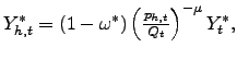
![$\displaystyle Y_{t}=\left[ \omega^{\frac{1}{\mu}}\left( Y_{h,t}\right) ^{\frac{\mu-1} {\mu}}+(1-\omega)^{\frac{1}{\mu}}\left( Y_{f,t}\right) ^{\frac{\mu-1}{\mu} }\right] ^{\frac{\mu}{\mu-1}},$](img54.gif) |
(12) |
where ![]() denotes the imports of Home from
Foreign. The demand functions for the home and foreign goods are
denotes the imports of Home from
Foreign. The demand functions for the home and foreign goods are
![]() and
and
![]() where
where ![]() and
and
![]() are the prices of the home and
foreign goods expressed in units of the home consumption basket,
and
are the prices of the home and
foreign goods expressed in units of the home consumption basket,
and ![]() is the real exchange rate. At the
aggregate level, the resource constraint takes into account not
only the consumption and investment of the native population (i.e.
is the real exchange rate. At the
aggregate level, the resource constraint takes into account not
only the consumption and investment of the native population (i.e.
![]() ) but also the
consumption of the immigrant workers established in Home,
) but also the
consumption of the immigrant workers established in Home,
![]() :
:
| (13) |
Immigrant workers' consumption, ![]() depends on
the optimization problem of the foreign household and on the
mechanism of remittances, which are described in the next
subsection.
depends on
the optimization problem of the foreign household and on the
mechanism of remittances, which are described in the next
subsection.
2.2 The Foreign Economy
Labor Migration We introduce cross-border labor mobility with sunk emigration
costs: foreign households have the option to work in the home
economy where wages are higher. The foreign household supplies a
total of
![]() units of labor every period.
Some household members reside and work abroad in Home,
units of labor every period.
Some household members reside and work abroad in Home, ![]() , whereas the rest work domestically in Foreign,
, whereas the rest work domestically in Foreign,
![]() , within the limit of the total
labor supply
, within the limit of the total
labor supply
![]() The
model calibration ensures that the immigrant wage in Home is higher
than the wage in the country of origin so that the incentive to
emigrate from Foreign to Home exists every period.9
However, a fraction of the foreign labor always remains in Foreign
(
The
model calibration ensures that the immigrant wage in Home is higher
than the wage in the country of origin so that the incentive to
emigrate from Foreign to Home exists every period.9
However, a fraction of the foreign labor always remains in Foreign
(
![]() 10 The
macroeconomic shocks are small enough for these conditions to hold
every period.
10 The
macroeconomic shocks are small enough for these conditions to hold
every period.
An amount ![]() of foreign labor emigrates to
Home every period, where the stock of immigrant labor is built
gradually over time. The time-to-build assumption in place implies
that the new immigrants start working one period after arriving at
the destination. They continue to work in Home in all subsequent
periods until the occurrence of an exogenous return-inducing shock,
which hits with probability
of foreign labor emigrates to
Home every period, where the stock of immigrant labor is built
gradually over time. The time-to-build assumption in place implies
that the new immigrants start working one period after arriving at
the destination. They continue to work in Home in all subsequent
periods until the occurrence of an exogenous return-inducing shock,
which hits with probability
![]() every period, forcing them to
return to the country of origin (Foreign). This shock occurs at the
end of every time period and may reflect issues such as termination
of employment in the destination economy, likelihood of
deportation, or voluntary return to the country of origin,
etc.11 Thus, the rule of motion for the
stock of immigrant labor in Home is:
every period, forcing them to
return to the country of origin (Foreign). This shock occurs at the
end of every time period and may reflect issues such as termination
of employment in the destination economy, likelihood of
deportation, or voluntary return to the country of origin,
etc.11 Thus, the rule of motion for the
stock of immigrant labor in Home is:
![]() where
where ![]() is the flow of new foreign labor that
emigrates to Home every period, and
is the flow of new foreign labor that
emigrates to Home every period, and ![]() is the
stock of immigrant labor that works in Home every period.
is the
stock of immigrant labor that works in Home every period.
Household's Problem The representative foreign household has preferences over real consumption and labor effort as in (2) and maximizes the inter-temporal utility:
 |
(14) |
subject to the budget constraint:
| (15) |
where
![]() is the wage in the foreign
economy and
is the wage in the foreign
economy and
![]() denotes the
total income from hours worked by the non-emigrant labor in
Foreign. We define
denotes the
total income from hours worked by the non-emigrant labor in
Foreign. We define ![]() as the immigrant wage
earned in Home, so that the total emigrant labor income expressed
in units of the foreign composite good is
as the immigrant wage
earned in Home, so that the total emigrant labor income expressed
in units of the foreign composite good is
![]() . On the spending
side, emigration requires a sunk cost of
. On the spending
side, emigration requires a sunk cost of ![]() units of immigrant labor, equal to
units of immigrant labor, equal to
![]() units of the foreign
composite. Changes in labor migration policies (i.e. border
enforcement) are reflected by shocks
units of the foreign
composite. Changes in labor migration policies (i.e. border
enforcement) are reflected by shocks
![]() to the level of the sunk
emigration cost
to the level of the sunk
emigration cost ![]() , so that
, so that
![]() . The gross
rental rate of foreign capital is denoted by
. The gross
rental rate of foreign capital is denoted by
![]() . Finally, capital accumulation
is characterized by:
. Finally, capital accumulation
is characterized by:
![]() , in which
, in which
![]() is a foreign
investment-specific shock.
is a foreign
investment-specific shock.
Optimality Conditions It is useful to rewrite the budget constraint as:
![]() where
where ![]() is the difference between the immigrant
wage in Home and the resident wage in Foreign at time
is the difference between the immigrant
wage in Home and the resident wage in Foreign at time ![]() , expressed in units of the foreign consumption basket:
, expressed in units of the foreign consumption basket:
| (16) |
The optimization problem of the foreign household delivers a typical Euler equation and pins down the total labor effort:
![$\displaystyle \frac{1}{\varepsilon_{t}^{I^{\ast}}}=\beta E_{t}\left[ \frac{\varsigma _{t+1}^{\ast}}{\varsigma_{t}^{\ast}}\left( r_{t+1}^{\ast}+\frac{1-\delta }{\varepsilon_{t+1}^{I^{\ast}}}\right) \right]$](img93.gif) and and 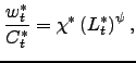 |
(17) |
where
 is the multiplier on the budget constraint and
![]() is a foreign
demand shock. In addition, potential emigrants face a trade-off
between the sunk emigration cost,
is a foreign
demand shock. In addition, potential emigrants face a trade-off
between the sunk emigration cost,
![]() , and the difference
between the stream of expected future wages at the destination,
, and the difference
between the stream of expected future wages at the destination,
![]() , and in the country of
origin,
, and in the country of
origin,
![]() , expressed in units of the
foreign composite good. Using the new budget constraint and the law
of motion for the stock of immigrant labor,
, expressed in units of the
foreign composite good. Using the new budget constraint and the law
of motion for the stock of immigrant labor,
![]() , the first order
condition with respect to new emigrant labor
, the first order
condition with respect to new emigrant labor ![]() sent abroad every period implies:
sent abroad every period implies:
![$\displaystyle f_{e,t}w_{i,t}Q_{t}^{-1}=\overset{\infty}{\underset{s=t+1}{\sum}}\left[ \beta(1-\delta_{l})\right] ^{s-t}E_{t}\left[ \left( \frac{\varsigma _{s}^{\ast}}{\varsigma_{t}^{\ast}}\right) d_{s}\right] .$](img102.gif) |
(18) |
The equation shows that, in equilibrium, the sunk emigration cost
equals the benefit from emigration, with the latter given by the
expected stream of future wage gains, ![]() ,
adjusted for the stochastic discount factor and the probability of
return to the country of origin every period.
,
adjusted for the stochastic discount factor and the probability of
return to the country of origin every period.
The Foreign Intermediate Good Foreign production is a Cobb-Douglas function of non-emigrant
labor and capital,
 , in which
![]() is a neutral
technology shock. As in Backus et al. (1994), the foreign-specific
good can be either used domestically,
is a neutral
technology shock. As in Backus et al. (1994), the foreign-specific
good can be either used domestically,
![]() or exported to the Home
economy,
or exported to the Home
economy, ![]() , so that the total foreign output is
, so that the total foreign output is
![]()
The foreign composite good,
![]() incorporates amounts of both
the foreign-specific intermediate good,
incorporates amounts of both
the foreign-specific intermediate good,
![]() and the home-specific
imported good,
and the home-specific
imported good,
![]() :
:
![$\displaystyle Y_{t}^{\ast}=\left[ \left( \omega^{\ast}\right) ^{\frac{1}{\mu}}\left( Y_{f,t}^{\ast}\right) ^{\frac{\mu-1}{\mu}}+(1-\omega^{\ast})^{\frac{1}{\mu} }\left( Y_{h,t}^{\ast}\right) ^{\frac{\mu-1}{\mu}}\right] ^{^{\frac{\mu }{\mu-1}}}.$](img112.gif) |
(19) |
This foreign composite good can be consumed by the non-emigrant labor that resides in Foreign (as opposed to the emigrant labor established in Home), invested in physical capital, and used for investment in emigration (to cover the sunk costs of sending new emigrant labor abroad):
| (20) |
The demand functions for the foreign and home goods in the
foreign economy are
![]() and
and
 where
where ![]() and
and
![]() are the corresponding
prices expressed in units of the foreign consumption basket. In
turn, the gross rental rate of foreign capital and the local wage
are determined by the marginal productivity of capital and labor,
are the corresponding
prices expressed in units of the foreign consumption basket. In
turn, the gross rental rate of foreign capital and the local wage
are determined by the marginal productivity of capital and labor,
 and
and
Remittances and Trade Balance The household's optimization problem pins down the fraction of
labor that resides abroad, ![]() and the
pooled level of consumption of the foreign household,
and the
pooled level of consumption of the foreign household,
![]() . Since the household is the
unit that maximizes utility in this model setup, the allocation of
consumption across emigrant and non-emigrant workers would remain
undetermined without further assumptions. To determine this
spending pattern, we introduce an insurance mechanism of
remittances parametrized to fit the data.
. Since the household is the
unit that maximizes utility in this model setup, the allocation of
consumption across emigrant and non-emigrant workers would remain
undetermined without further assumptions. To determine this
spending pattern, we introduce an insurance mechanism of
remittances parametrized to fit the data.
We assume that immigrant workers residing in Home send
remittances, denoted with ![]() , to Foreign
every period. Thus, the immigrant labor income is divided entirely
between remittances sent to Foreign (which are expressed in units
of the foreign composite) and immigrant consumption taking place in
Home,
, to Foreign
every period. Thus, the immigrant labor income is divided entirely
between remittances sent to Foreign (which are expressed in units
of the foreign composite) and immigrant consumption taking place in
Home,
![]() .12 To
highlight the intensive and extensive margins of remittances, we
also consider remittances per unit of immigrant labor defined as
.12 To
highlight the intensive and extensive margins of remittances, we
also consider remittances per unit of immigrant labor defined as
![]() where
where
![]() is consumption per
unit of immigrant labor. The stock of established immigrants,
is consumption per
unit of immigrant labor. The stock of established immigrants,
![]() , represents the extensive margin of
remittances.
, represents the extensive margin of
remittances.
The risk sharing mechanism of remittances is described in detail
in Appendix B. In summary, the mechanism warrants a steady-state
allocation in which foreign household members residing in either
Home or Foreign enjoy the same amount of consumption per unit of
labor, equal to
![]() units of consumption.13 Thus, the steady-state amount of
remittances per unit of immigrant labor is equal to the difference
between the immigrant wage and immigrant consumption (expressed in
units of the composite good in Home):
units of consumption.13 Thus, the steady-state amount of
remittances per unit of immigrant labor is equal to the difference
between the immigrant wage and immigrant consumption (expressed in
units of the composite good in Home):
![]() .
.
The sunk migration cost is a market friction that renders the stock of immigrant labor a state variable that cannot adjust immediately to temporary shocks. As a result, the gap between the immigrant and foreign wages varies over the business cycle, and household members working on both sides of the border obtain either a net surplus or a loss relative to the steady-state allocation of consumption. As shown in Appendix B, remittances represent an altruistic compensation mechanism between immigrant and resident workers:
 with with |
(21) |
A positive value of ![]() implies that a
relative improvement in the purchasing power of the immigrant wage
in terms of the consumption basket in Home (where immigrant
consumption takes place) or a relative deterioration of the
purchasing power of the foreign wage in terms of the foreign
consumption basket trigger an altruistic increase in
remittances.14 The magnitude of
implies that a
relative improvement in the purchasing power of the immigrant wage
in terms of the consumption basket in Home (where immigrant
consumption takes place) or a relative deterioration of the
purchasing power of the foreign wage in terms of the foreign
consumption basket trigger an altruistic increase in
remittances.14 The magnitude of ![]() characterizes the thrust of the altruistic
motive.15
characterizes the thrust of the altruistic
motive.15
The current account balance for Home is:
![]() Under financial autarky, the balanced current account condition,
Under financial autarky, the balanced current account condition,
![]() , implies that the trade balance,
, implies that the trade balance,
![]() must equal
the amount of remittances,
must equal
the amount of remittances,
![]() . In the absence of financial
integration, remittances act as a substitute for contingent claims
in smoothing income flows.
. In the absence of financial
integration, remittances act as a substitute for contingent claims
in smoothing income flows.
2.3 Shocks
Structural shocks that characterize the business cycle in our
model are assumed to follow ![]() processes with
i.i.d. normal error terms,
processes with
i.i.d. normal error terms,
![]() , in which
, in which
![]() and
and
![]() , where
, where
![]() As in Lubik and Schorfheide (2005), domestic and foreign shocks
are independent.
As in Lubik and Schorfheide (2005), domestic and foreign shocks
are independent.
2.4 Financial Integration
Appendix A considers the case of financial integration. We assume that international asset markets are incomplete, and that households trade country-specific, risk-free bonds. Under financial integration, a trade deficit can be financed by either remittances or international borrowing. Therefore, the current account balance for Home (i.e. the trade balance plus financial investment income minus the outflow of remittances) must equal the negative of the financial account balance (i.e. the change in bond holdings).
3 Bayesian Estimation
The Bayesian estimation technique uses a general equilibrium approach that addresses the identification problems of reduced form models. It is a system-based analysis that fits the solved DSGE model to a vector of aggregate time series (see Fernandez-Villaverde and Rubio-Ramirez, 2004, or Lubik and Schorfheide, 2005, for additional details).16
Data The number of data series used in the estimation cannot exceed the number of structural shocks in the model. Therefore, we use seven data series for the U.S. and Mexico during the period 1980:1 to 2004:3, consisting of real GDP, real consumption and real investment for each economy, as well as the total number of hours that U.S. border officers spent patrolling the border as a proxy for the intensity of border enforcement.17 We interpret an increase in border patrol hours as an increase in border enforcement. We seasonally adjust the data series using the X-12 ARIMA method, a method which addresses the important seasonal components in the labor migration and border apprehensions data. The deseasonalized data is expressed in natural logs, then detrended with a cubic trend and finally first-differenced to obtain growth rates.18 The solid line in Fig. 3 depicts the data that we match with the model.
We use additional data (beyond that included in the structural
estimation) to validate the model fit and to estimate parameters
that otherwise would remain unidentified. First, we consider data
on U.S.-Mexico relative unskilled wages as well as data on workers'
remittances expressed in real Mexican pesos. For the U.S., we use
the real hourly wage for workers with fewer than 12 years of
education (i.e. less than high school degree). For Mexico, we
consider the real hourly wage in the maquiladora sector.
However, the data on relative unskilled wages and remittances is
available for a time span that is too short to be included in the
Bayesian estimation. Instead, we use the detrended series to
estimate the elasticity of remittances with respect to the
unskilled wage differential ![]() , depicted in
equation (21),
in a reduced form estimation over the interval 1995:1 to
2006:3.
, depicted in
equation (21),
in a reduced form estimation over the interval 1995:1 to
2006:3.
Second, we use the number of apprehensions (arrests) at the U.S.-Mexico border to evaluate the model, but we do not include these in the structural estimation for two reasons. One reason is that the apprehensions data (depicted in Fig. 1) are noisy due to the random nature of border interceptions and arrests, and therefore can serve only as a rough proxy for the flows of emigrant labor. The other reason is an identification problem regarding the effect of border enforcement on apprehensions. In this paper, we assume that an increase in border enforcement (reflected by U.S. border patrol hours) leads to an increase in the sunk emigration cost. As documented by Orrenius (2001), changes in border enforcement policy act mainly as a deterrent strategy for migration flows. Migrants are more likely to hire human smugglers (coyotes) when they perceive an increase in border enforcement. The coyotes also face greater challenges in border crossings due to the increase in enforcement, and therefore they raise their fees. Consequently, the increase in border enforcement increases the cost of labor migration, which in turn may reduce the size of labor migration flows. However, for the same number of attempted illegal crossings, an increase in border patrol hours may result in more arrests. Because border enforcement may affect both the number of crossings and the number of arrests, and because the actual number of attempted crossings is unknown, it is impossible to disentangle the effect of enforcement from that of crossings on total apprehensions.
Bearing these issues in mind, we treat the flow of new emigrant
labor (![]() ) as a latent variable in our
estimated model. We use the Kalman filter to write the likelihood
function of the data and estimate the structural parameters. This
procedure allows to asses the type and magnitude of the shocks
faced by the two economies during the sample period. The
reconstruction of these " smoothed'' shocks allows us to make
inference about this latent variable. In what follows, we compare
the moments and autocovariance functions of this revealed latent
variable with those of the actual data on apprehensions to grasp
some insight of the model fit. Similarly, remittances also are
treated as a latent variable, given that the short length of this
data series does not allow for its use in the structural
estimation.
) as a latent variable in our
estimated model. We use the Kalman filter to write the likelihood
function of the data and estimate the structural parameters. This
procedure allows to asses the type and magnitude of the shocks
faced by the two economies during the sample period. The
reconstruction of these " smoothed'' shocks allows us to make
inference about this latent variable. In what follows, we compare
the moments and autocovariance functions of this revealed latent
variable with those of the actual data on apprehensions to grasp
some insight of the model fit. Similarly, remittances also are
treated as a latent variable, given that the short length of this
data series does not allow for its use in the structural
estimation.
Calibration Some parameters are fixed in the estimation:
![]() is the discount factor;
is the discount factor;
![]() is the share of capital in
output;
is the share of capital in
output;
![]() is the depreciation rate of the
capital stock. These parameters are difficult to identify unless
capital stock data is included in the measurement equation. The
rate at which the established immigrant labor returns to the
country of origin is not identified either. We set the quarterly
immigrant return rate at
is the depreciation rate of the
capital stock. These parameters are difficult to identify unless
capital stock data is included in the measurement equation. The
rate at which the established immigrant labor returns to the
country of origin is not identified either. We set the quarterly
immigrant return rate at
![]() , which on average reflects
the findings in Reyes (1997) that approximately 50% of undocumented
Mexican immigrants return to their country of origin within two
years after their arrival in the U.S. (which corresponds to a
quarterly exit rate of 0.0635) and that 65% of immigrants return
within four years after arrival (i.e. quarterly exit rate of
0.0830).19The degree of home bias,
, which on average reflects
the findings in Reyes (1997) that approximately 50% of undocumented
Mexican immigrants return to their country of origin within two
years after their arrival in the U.S. (which corresponds to a
quarterly exit rate of 0.0635) and that 65% of immigrants return
within four years after arrival (i.e. quarterly exit rate of
0.0830).19The degree of home bias, ![]() is not identified since spending ratios are not part
of the measurement set. As in Backus et al. (1994), we set
is not identified since spending ratios are not part
of the measurement set. As in Backus et al. (1994), we set
![]() , while allowing for a slightly
higher degree of openness for the smaller foreign economy,
, while allowing for a slightly
higher degree of openness for the smaller foreign economy,
![]() . Finally, we define the
pool of native unskilled labor to include the adult U.S. population
active in the labor force that lacks a high school degree. Using
data from the U.S. Census Bureau (2007), we set the share of
unskilled labor at
. Finally, we define the
pool of native unskilled labor to include the adult U.S. population
active in the labor force that lacks a high school degree. Using
data from the U.S. Census Bureau (2007), we set the share of
unskilled labor at
![]() Finally, we set the weight on
the utility of representative skilled household
Finally, we set the weight on
the utility of representative skilled household
![]() , so that the consumption ratio
for the home representative skilled and unskilled households
matches the corresponding wage ratio,
, so that the consumption ratio
for the home representative skilled and unskilled households
matches the corresponding wage ratio,
![]() 20 We
base our assumption on the findings in Krueger and Perri (2007)
that differences in the consumption of population groups with
different levels of educational attainment (e.g. skilled and
unskilled) closely reflect the income differences between the
respective groups. The calibrated parameters are depicted in Table
1.
20 We
base our assumption on the findings in Krueger and Perri (2007)
that differences in the consumption of population groups with
different levels of educational attainment (e.g. skilled and
unskilled) closely reflect the income differences between the
respective groups. The calibrated parameters are depicted in Table
1.
Prior Distributions The remaining parameters are estimated. The first four columns
of Table 2 present the mean and the standard deviation of the prior
distributions, together with their respective density functions. We
do not have much prior information about the magnitude of shocks.
Therefore, the variances of all shocks are harmonized as in Smets
and Wouters (2007), and assumed to follow an Inverse Gamma
distribution that delivers a relatively large domain. The
autoregressive parameters in the shocks are assumed to follow a
Beta distribution that covers the range between 0 and 1. For these,
we select rather strict standard deviations and thus have tight
prior distributions in order to obtain a clear separation between
persistent and non-persistent shocks, and also to generate
volatilities for the endogenous variables that are broadly in line
with the data (See Smets and Wouters, 2003, for details). For the
remaining parameters we consider Beta or Gamma distributions, which
are restricted to the positive support. We set a relatively loose
prior for the elasticity of substitution between the home and
foreign goods ![]() centered at 1.5, the value in Backus
et al. (1994). We set the prior mean of
centered at 1.5, the value in Backus
et al. (1994). We set the prior mean of ![]() at 1,
which delivers a Frisch elasticity of labor supply that is in
between microeconomic estimates and the relative larger values
usually observed in the macro literature. As discussed in the
previous section, the reduced form estimation of equation (21) sets the prior
for the elasticity of remittances with respect to the wage
differential
at 1,
which delivers a Frisch elasticity of labor supply that is in
between microeconomic estimates and the relative larger values
usually observed in the macro literature. As discussed in the
previous section, the reduced form estimation of equation (21) sets the prior
for the elasticity of remittances with respect to the wage
differential ![]() at
at ![]() .
.
We are left with five parameters to estimate, namely ![]() (share of unskilled labor in output)
(share of unskilled labor in output)![]()
![]() (elasticity of substitution between
capital and unskilled labor)
(elasticity of substitution between
capital and unskilled labor)![]()
![]() (relative productivity of native skilled over
unskilled)
(relative productivity of native skilled over
unskilled)![]()
![]() (sunk
emigration cost level), and
(sunk
emigration cost level), and ![]() (elasticity of
substitution between capital and skilled labor). For the first four
parameters, we center the priors to match four equilibrium
allocations in steady state: (1) The share of Mexico's labor force
residing in the U.S. is
(elasticity of
substitution between capital and skilled labor). For the first four
parameters, we center the priors to match four equilibrium
allocations in steady state: (1) The share of Mexico's labor force
residing in the U.S. is
![]() (Hanson, 2006).
(2) Remittances represent the equivalent of
(Hanson, 2006).
(2) Remittances represent the equivalent of ![]() of
Mexico's GDP.21 (3) The ratio between the wages of
the native skilled and unskilled labor in the U.S. is
of
Mexico's GDP.21 (3) The ratio between the wages of
the native skilled and unskilled labor in the U.S. is
![]() . (4) The U.S.-Mexico
share of GDP per capita expressed in purchasing power parity terms
is
. (4) The U.S.-Mexico
share of GDP per capita expressed in purchasing power parity terms
is ![]() , as shown by data from the IMF's World
Economic Outlook. To this end, we choose
, as shown by data from the IMF's World
Economic Outlook. To this end, we choose
![]() ,
,
![]() ,
, ![]() and
and
![]() . As previously discussed, we base
the assumption that
. As previously discussed, we base
the assumption that
![]() on the findings of Krusell et
al. (2000) that skilled labor and capital are relative complements.
Krusell et al. (2000) document a high complementarity between
skilled labor (i.e. college graduates) and capital, whereas our
pool of skilled workers is much larger since we also include high
school graduates. Therefore, we center the priors for
on the findings of Krusell et
al. (2000) that skilled labor and capital are relative complements.
Krusell et al. (2000) document a high complementarity between
skilled labor (i.e. college graduates) and capital, whereas our
pool of skilled workers is much larger since we also include high
school graduates. Therefore, we center the priors for ![]() at 0.85, a value which is only slightly below the prior
assigned to
at 0.85, a value which is only slightly below the prior
assigned to ![]() Based on the capital-skill
complementary assumption, we choose rather tight priors for these
parameters.
Based on the capital-skill
complementary assumption, we choose rather tight priors for these
parameters.
Estimation Results (Posterior
Distributions) The last five columns of Table 2 report the posterior mean,
mode, and standard deviation obtained from the Hessian, along with
the 90% probability interval of the structural parameters. The
priors are informative in general. Noticeably, we find that
![]() and
and ![]() are
significantly closer to each other (0.91 and 0.94) despite the
tight prior, weakening further the implied capital-skill
complementarity. Since remittances are not part of the estimation
set,
are
significantly closer to each other (0.91 and 0.94) despite the
tight prior, weakening further the implied capital-skill
complementarity. Since remittances are not part of the estimation
set, ![]() is not identified. As a result, its
posterior distribution practically replicates the prior based on a
reduced form estimation. The estimated values for
is not identified. As a result, its
posterior distribution practically replicates the prior based on a
reduced form estimation. The estimated values for ![]() and
and ![]()
![]() and
and
![]() are remarkably higher than their
priors, indicating a larger degree of substitution between the U.S.
and Mexican goods and also a value of the labor supply elasticity
that is closer to the microeconomic estimates. The posterior for
the level of sunk migration costs,
are remarkably higher than their
priors, indicating a larger degree of substitution between the U.S.
and Mexican goods and also a value of the labor supply elasticity
that is closer to the microeconomic estimates. The posterior for
the level of sunk migration costs, ![]() is
5.52, significantly higher than its prior, indicating that the sunk
cost per unit of emigrant labor is equivalent to the immigrant
labor income obtained over six quarters in the destination economy.
Note that border enforcement shocks are persistent and volatile (
is
5.52, significantly higher than its prior, indicating that the sunk
cost per unit of emigrant labor is equivalent to the immigrant
labor income obtained over six quarters in the destination economy.
Note that border enforcement shocks are persistent and volatile (
![]()
![]() and also that the neutral
technology innovations are less persistent and more volatile in
Mexico than in the U.S. (
and also that the neutral
technology innovations are less persistent and more volatile in
Mexico than in the U.S. (
![]() and
and
![]() in the U.S., compared to
in the U.S., compared to
![]() and
and
![]() in Mexico).
in Mexico).
4 Model Fit and the Role of Border Enforcement
Model Fit Fig. 3 reports the benchmark model's Kalman filtered one-sided estimates computed at the posterior (dashed line) along the data. The model fit appears to be satisfactory. Table 3 reports unconditional moments for the actual data. As with the vector of observables, we also express the data series in growth rates. We report standard deviations and first-order autocorrelations for three series that reflect key variables of our model: border apprehensions, remittances and U.S. border patrol hours.22 These data series are highly volatile. In addition, changes in border patrol hours are somewhat persistent. Next we report the correlations of these three data series with: (1) the U.S.-Mexico ratio of real GDP, (2) real GDP in the U.S. and (3) real GDP in Mexico, in which the GDP in Mexico is adjusted by the bilateral real exchange rate. In the data, apprehensions and remittances are pro-cyclical with the U.S.-Mexico GDP ratio, counter-cyclical with Mexico's GDP and pro-cyclical with the U.S. GDP. However, for apprehensions, the correlation with the U.S. GDP is significantly small. The link between border patrol hours and macroeconomic performance is particularly weak as the correlation of this variable with either (1), (2) or (3) is close to zero. This possibly indicates that the degree of border enforcement is a political decision often unaffected by macroeconomic considerations.
Table 4 reports the median (along the 5th and 95th percentiles)
from the simulated distributions of moments using the samples
generated with parameter draws from the posterior distribution. In
general, the model delivers volatility and persistence values that
are fairly close to observed values. The model fails, however, to
match the high volatility of remittances and the persistence of
border enforcement, despite the high persistence of enforcement
shocks in the estimated model. The model captures particularly well
the co-movement of the key migration indicators (labor migration
and remittances) with the relative economic performance of the U.S.
and Mexico. Namely, the correlation of the Home-Foreign GDP ratio
with either remittances (![]() ) or migration flows
(
) or migration flows
(![]() ) is positive and significant. The
correlation is higher for remittances than for migration flows, a
result which is in line with the data. In addition, the model
delivers a correlation of border enforcement with the output ratio
as well as with output in either Home or Foreign that is close to
zero, as in the data.
) is positive and significant. The
correlation is higher for remittances than for migration flows, a
result which is in line with the data. In addition, the model
delivers a correlation of border enforcement with the output ratio
as well as with output in either Home or Foreign that is close to
zero, as in the data.
Labor migration flows are negatively correlated with the foreign GDP, whereas their correlation with the home GDP is not significantly different than zero. This finding is consistent with the data and may be indicative of the inability of the stock of immigrants to react to domestic shocks. In addition, remittances are positively correlated with home output whereas their correlation with foreign output is negative but relatively small in absolute terms. Finally, notice that so far we have compared the empirical moments to their model counterparts expressed in growth rates, whereas the data plotted in Fig. 1 and Fig. 2 is in percentage deviations from the trend. When we compute the theoretical moments of variables expressed as log deviations from steady state, the correlation of labor migration and remittances with the Home-Foreign GDP ratio are 0.30 and 0.70, which are close to the corresponding empirical correlations (0.44 and 0.75 respectively).
To further assess the model adequacy, we compare the vector
autocovariance functions in the model and in the data, as in
Adolfson et al. (2007). The function depicts the covariance of each
observable variable against itself (measured at lags
![]() ) and other variables. These
functions are computed by estimating an unrestricted VAR model with
both the U.S.-Mexico data and artificial data sets of the same time
length generated through model simulations with parameter draws
from the posterior. We include output for both economies, border
enforcement and apprehensions/migration flows.23 Fig. 4 displays
the median vector autocovariance function from the DSGE
specification (thin line), along with the 2.5 and 97.5 percentiles
for the mentioned subset of variables. The posterior intervals for
the vector autocovariance are wide. In this case, this range
reflects both parameter and sample uncertainty, which in the latter
case is the result of using relatively few observations in the
computations. Nonetheless, in general, the data covariances (thick
lines) fall within the error bands, indicating that the model is
somewhat able to replicate the cross-variances in the data.
Overall, the model fit is satisfactory, particularly when taking
into consideration that neither migration flows nor remittances are
part of the data that we use in the Bayesian estimation.
) and other variables. These
functions are computed by estimating an unrestricted VAR model with
both the U.S.-Mexico data and artificial data sets of the same time
length generated through model simulations with parameter draws
from the posterior. We include output for both economies, border
enforcement and apprehensions/migration flows.23 Fig. 4 displays
the median vector autocovariance function from the DSGE
specification (thin line), along with the 2.5 and 97.5 percentiles
for the mentioned subset of variables. The posterior intervals for
the vector autocovariance are wide. In this case, this range
reflects both parameter and sample uncertainty, which in the latter
case is the result of using relatively few observations in the
computations. Nonetheless, in general, the data covariances (thick
lines) fall within the error bands, indicating that the model is
somewhat able to replicate the cross-variances in the data.
Overall, the model fit is satisfactory, particularly when taking
into consideration that neither migration flows nor remittances are
part of the data that we use in the Bayesian estimation.
The Role of Border Enforcement Table 5 reports counterfactual correlations, obtained by using
the posterior median of the estimated parameters while altering
only the steady-state level of the sunk emigration cost ![]() . We consider two alternative scenarios with low and
high border enforcement
. We consider two alternative scenarios with low and
high border enforcement ![]() and
and ![]() The latter scenario closely resembles the one in
the estimation
The latter scenario closely resembles the one in
the estimation
![]() .24
.24
Note that when migration barriers are low, the labor migration flows are more responsive to business cycles. In the case with low sunk cost, the correlation of the GDP ratio with migration flows is 0.51. In the case with high sunk cost, the correlation of the GDP ratio with migration flows declines (0.27) whereas the correlation with Home GDP is only 0.01. It is also notable that in the case with low migration barriers, remittances are correlated less with Mexican GDP, indicating that, when restrictions to labor mobility are low, the gap between the immigrant wage in Home and the equivalent wage in Foreign is relatively small. Thus, the need for remittances as a compensation mechanism is limited.
Simulation results also indicate that migration barriers significantly affect the volatility of the immigrant wage and total remittances. With low border enforcement, the standard deviations of these two variables (this time expressed in log deviations from steady state rather than in growth rates) are 1.59 and 2.18, respectively. With high border enforcement, the volatility of the immigrant wage and remittances increases to 2.62 and 2.64. In summary, as migration barriers restrict the ability of the stock of immigrant labor to adjust over the cycle, its factor payments and the associated remittances become more volatile.
5 The Effect of Shocks
5.1 Impulse Response Functions
We consider the impulse responses of key model variables to temporary shocks to border enforcement and neutral technology. In the latter case, we also consider a series of counterfactual scenarios (high vs. low sunk cost, financial autarky vs. integration).25
Positive Shock to Border Enforcement Fig. 5 reports the median impulse response of the estimated
model (along the 10th and 90th percentiles) to a positive shock to
the sunk emigration cost (one standard deviation), reflecting an
increase in border enforcement. As previously discussed, this
estimated shock remains very persistent. The increase in the sunk
emigration cost leads to a decline in the arrivals and in the stock
of immigrant labor, which in turn generates a gradual decline in
the capital stock in Home. This translates into lower home output
and aggregate consumption (defined as
![]() . Notice, however, that the wage
of established immigrants (which is the same as that of native
unskilled labor) benefits from this policy change.
. Notice, however, that the wage
of established immigrants (which is the same as that of native
unskilled labor) benefits from this policy change.
As foreign workers are deterred from emigrating to Home, the resident labor supply in Foreign becomes relatively abundant, and the foreign wage falls. The cheaper labor input encourages capital accumulation and enhances output in Foreign. However, due to the misallocation of labor across borders, the pooled consumption of the foreign household declines. The flow of remittances per unit of labor significantly increases to compensate for the wage difference between Home and Foreign. Total remittances decrease slightly as the immigrant labor stock declines.
Positive Technology Shock in Home: Low vs. High Sunk Emigration Costs We consider the two counterfactual scenarios with low and high
sunk emigration costs: ![]() (solid line) and
(solid line) and
![]() (dashed line). In this experiment,
different levels of migration barriers result in different
steady-state levels for the model variables. For consistency, we
compute the impulse responses using the posterior median of the
estimated parameters (with the only exception of
(dashed line). In this experiment,
different levels of migration barriers result in different
steady-state levels for the model variables. For consistency, we
compute the impulse responses using the posterior median of the
estimated parameters (with the only exception of ![]() and plot them as percentage deviations from steady
state. Fig. 6 shows the effect of an unexpected 1% increase in home
productivity.
and plot them as percentage deviations from steady
state. Fig. 6 shows the effect of an unexpected 1% increase in home
productivity.
Following the positive shock, the rise in the wage premium
encourages the arrival of new immigrant labor (![]() ). The immigrant wage premium and immigrant entry
persist above their steady-state levels after the initial shock,
and thus the stock of established immigrant labor (
). The immigrant wage premium and immigrant entry
persist above their steady-state levels after the initial shock,
and thus the stock of established immigrant labor (![]() ) adjusts gradually over time. Notably, the stock of
immigrant labor increases relatively less in the economy with the
higher sunk migration cost. In turn, the relative scarcity of
immigrant labor causes the immigrant wage in Home (which is the
same as the domestic unskilled wage) to increase more. Therefore,
as the foreign household attempts to smooth consumption across
members residing in both countries, the amount of remittances per
immigrant worker increases by more in the model with the higher
sunk cost. In the foreign economy, the local wage increases by less
in the scenario with the higher sunk migration cost. The result is
due to the larger fraction of labor that remains in Foreign when
emigration is more costly, in turn enhancing capital accumulation
and output in Foreign.
) adjusts gradually over time. Notably, the stock of
immigrant labor increases relatively less in the economy with the
higher sunk migration cost. In turn, the relative scarcity of
immigrant labor causes the immigrant wage in Home (which is the
same as the domestic unskilled wage) to increase more. Therefore,
as the foreign household attempts to smooth consumption across
members residing in both countries, the amount of remittances per
immigrant worker increases by more in the model with the higher
sunk cost. In the foreign economy, the local wage increases by less
in the scenario with the higher sunk migration cost. The result is
due to the larger fraction of labor that remains in Foreign when
emigration is more costly, in turn enhancing capital accumulation
and output in Foreign.
Given the model symmetry, a negative productivity shock leads to an economic recession with opposite results. The slower decline in the stock of immigrant labor resembles a lock-in effect that puts additional downward pressure on the wage and employment of the native unskilled. In summary, a less flexible immigration policy reflected by a larger sunk migration costs enhances the volatility of the native unskilled wage, the immigrant wage and remittances per unit of immigrant labor in response to productivity shocks.
Positive Technology Shock in Home: Financial Autarky vs. Integration Fig. 7 displays the impulse responses computed at the posterior median parameter estimates of the benchmark model. In the model with financial integration, the one period, risk-free bond constitutes an additional instrument (other than migration and remittances) that foreign households use to smooth their inter-temporal consumption path and diversify away from country-specific risk. That is, foreign households have the option to lend abroad as an alternative to investing in emigration.
Following a transitory, 1% increase in home productivity,
international bond trading (dashed line) generates a notably more
muted increase in the arrival of new immigrant labor (![]() ) relative to the case with financial autarky (solid
line). Financial integration allows for capital to flow towards the
economy with a relatively higher rate of return (Home), whose trade
balance becomes negative on impact. Immediately after the shock, as
foreign households lend to Home, they invest less in emigration to
Home. However, as capital accumulation enhances labor productivity
and wages in Home, the immigrant labor entry recovers in the medium
run. The entry of immigrant labor under financial integration
catches up with immigrant entry under financial autarky 20 quarters
after the initial shock.
) relative to the case with financial autarky (solid
line). Financial integration allows for capital to flow towards the
economy with a relatively higher rate of return (Home), whose trade
balance becomes negative on impact. Immediately after the shock, as
foreign households lend to Home, they invest less in emigration to
Home. However, as capital accumulation enhances labor productivity
and wages in Home, the immigrant labor entry recovers in the medium
run. The entry of immigrant labor under financial integration
catches up with immigrant entry under financial autarky 20 quarters
after the initial shock.
5.2 Forecast Error Variance Decomposition
Fig. 8 displays the forecast error variance decomposition of the seven observables used in the estimation, plus remittances and migration flows at various horizons (Q1, Q4, Q16, Q40), based on the posterior benchmark estimation. Technology shocks aggregate the effects of both neutral and investment-specific shocks. As discussed in Justiniano et al. (2009), the investment shock affects the marginal efficiency of investment, and it can be linked to more fundamental disturbances to the functioning of the financial system that negatively affect productivity but are not explicitly included in the model. Changes affecting border enforcement, which are assumed to be exogenous, and demand shocks complete the list.
In the short run (within a year), we observe that demand shocks play a primary role in driving the dynamics of the real macroeconomic variables in the U.S., which is in line with evidence in Smets and Wouters (2007). While the demand shocks are relatively less important to explain output in Mexico at short horizons, their impact on consumption is nonetheless sizable. In the medium to long-run, technology shocks are dominant drivers of output, consumption and investment in both countries.
At all horizons, Mexican technology and border enforcement shocks are the most important drivers of labor migration flows. In the short run, technology innovations in Mexico dominate (explain more than 70% of the forecast error variance at Q1), whereas the border enforcement shocks become relatively more important in the medium to long-run. Technology shocks in the U.S. play a negligible role in the migration dynamics, which is consistent with the lock-in effect that makes the stock of immigrant labor non-reactive to macroeconomic developments in the destination economy.
At short horizons, technology shocks and, to some extent, demand shocks explain practically all the variability of remittances. Remittances are reactive to shocks originating on both sides of the border, a result which highlights its insurance role. Instead, in the long-run, the forecast error variance of remittances is explained mostly by border enforcement and technology in Mexico, indicating that remittances are linked to the labor migration developments at longer horizons.
5.3 Historical Decomposition
Fig. 9 shows the historical contributions of shocks to the growth of key variables over the sample period (output in Mexico, border enforcement and labor migration). For the first two variables, the actual growth data (expressed as deviation from trend growth) is displayed. As previously explained, we apply the Kalman smoothing procedure to reconstruct the historical contributions of shocks to the labor migration flows as a latent variable.
The historical evidence indicates that output in Mexico (panel 1) was subject to several negative technology shocks of sizable magnitudes throughout the sample period. The debt crisis of 1982 led to a dramatic reversal in the earlier pattern of economic growth. The subsequent recovery was interrupted in late 1985, following a massive earthquake that hit Mexico City in September. As a result, output remained subdued until late 1986. Mexican output displays the sharpest decline in 1995 in the aftermath of the " tequila crisis.'' Finally, as the U.S. economy slowed down in late 2000, the Mexican economy fell into a mild recession in 2001, and output growth remained below trend until 2003.
Next we depict the detrended number of U.S. border patrol hours (panel 2), which is a proxy for border enforcement. The time series is characterized by persistent swings: border enforcement registered a sharp increase in 1989, and another steady increase in the second half of the 1990s. Enforcement was relaxed temporarily in late 2001, but a tightening followed at the end of 2002.
Finally, we estimate the contribution of historical shocks to labor migration flows and use them to make inference on this latent variable (panel 3). When compared with the actual number of apprehensions (Fig. 1), the model captures the increase in apprehensions in the aftermath of the debt crisis of 1982, and also the increase triggered by the recession that followed the Mexico City earthquake in 1985. In 1989, apprehensions declined sharply without an economic reason, reflecting a large increase in border enforcement that acted as a migration deterrent. In particular, the model succeeds in accounting for the sharp increase in apprehensions after the " tequila crisis" episode in 1995. Finally, the model captures the sharp increase in border apprehensions that began in early 2002, the result of both a relaxation in border enforcement and recession in Mexico.
6 Welfare Implications of Labor Mobility Restrictions
The planner maximizes welfare in Home, which is defined as the household's stream of expected utility. Policies that restrict labor mobility affect welfare in the destination economy through two different channels. First, since the native unskilled labor input is scarce and not perfectly substitutable in production, higher migration barriers deter capital accumulation. This, in turn, decreases labor productivity, wages and consumption. Business cycles fluctuations are not an issue in this case, and welfare can be computed in a static deterministic framework. Second, migration barriers lead to additional labor misallocations in the presence of aggregate shocks, as the stock of immigrant labor is slow to adjust over the course of the business cycle. Clearly, the second channel is the focus of this paper.
To distinguish between these two channels, we first perform the
welfare analysis while turning off all aggregate shocks and
focusing on the steady-state analysis of the estimated model. We
consider two counterfactual scenarios, with low ![]() and high
and high ![]() levels of border
enforcement, and compare their welfare outcomes to that of the
estimated model (with
levels of border
enforcement, and compare their welfare outcomes to that of the
estimated model (with
![]() ). We also analyze the welfare
outcomes while incorporating all the estimated stochastic shocks in
the counterfactual scenarios. Here we solve the model using a
second-order approximation to the model equilibrium relationships
around the deterministic steady state, following the methods in
Schmitt-Grohé and Uribe (2004).26
). We also analyze the welfare
outcomes while incorporating all the estimated stochastic shocks in
the counterfactual scenarios. Here we solve the model using a
second-order approximation to the model equilibrium relationships
around the deterministic steady state, following the methods in
Schmitt-Grohé and Uribe (2004).26
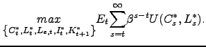
Welfare in the Home economy is defined as:
![$\displaystyle W_{t}=E_{t}\left[ \overset{\infty}{\underset{s=t}{\sum}}\beta^{s-t}\left\{ \phi sU\left( c_{s,t},l_{s,t}\right) +\left( 1-\phi\right) \left( 1-s\right) U\left( c_{u,t},l_{u,t}\right) \right\} \right] . $](img215.gif)
As standard, we measure the welfare cost (or gain) relative to
our benchmark estimated model as the fraction of the expected
aggregate consumption stream that one should add (or extract) so
that households are indifferent between the benchmark estimated
model and each of the two counterfactual scenarios. Since the
planner allocates consumption proportionally:
![]() in every
period
in every
period ![]() we can abstract from distributional
issues across the skilled and unskilled households in Home.
we can abstract from distributional
issues across the skilled and unskilled households in Home.
Our results indicate that a transition from the benchmark estimated model to the scenario with low migration barriers leads to a gain of 3.63% of the consumption stream in steady state (Table 6). When shocks are incorporated in the picture, the welfare gains of reducing barriers are significantly larger (4.36% gain). In the context of the literature, the difference between the two values is large and can be linked to the misallocation of labor across the border when the two economies are subject to shocks, some of which are highly persistent and volatile.27
On the contrary, moving from the estimated baseline framework to
the scenario with high migration barriers results in a 0.52% loss
in the consumption stream. This loss is amplified when adding the
stochastic shocks (0.67 loss). Interestingly, migration barriers
are already high in the benchmark estimated model (i.e.
![]() ), indicating that even a moderate
tightening in border enforcement can lead to significant losses
when the pool of unskilled labor is already constrained.
), indicating that even a moderate
tightening in border enforcement can lead to significant losses
when the pool of unskilled labor is already constrained.
Alternative Scenario with High Share of Native Unskilled The baseline model calibration reflects the relatively low share
of the U.S. labor force that holds no high school degree, currently
at only 8% (i.e. ![]() ). This percentage is the
result of the steady increase in high school enrollments between
the postwar era and the late 1970s. As an alternative to the
baseline calibration, we consider a scenario in which the share of
native unskilled labor in the destination economy represents as
much as 25% of the total. We find that lowering the sunk
immigration cost from the estimated value of
). This percentage is the
result of the steady increase in high school enrollments between
the postwar era and the late 1970s. As an alternative to the
baseline calibration, we consider a scenario in which the share of
native unskilled labor in the destination economy represents as
much as 25% of the total. We find that lowering the sunk
immigration cost from the estimated value of
![]() to
to ![]() leads
to a 1.01% gain in the consumption stream in steady state, due to
the improved availability of unskilled labor (both native and
immigrant). Instead, further tightening the border
leads
to a 1.01% gain in the consumption stream in steady state, due to
the improved availability of unskilled labor (both native and
immigrant). Instead, further tightening the border ![]() to
to ![]() has no impact on the domestic
household's welfare.
has no impact on the domestic
household's welfare.
However, when we extend the welfare analysis to incorporate the effect of shocks, the welfare gains of lowering the sunk immigration are reduced to only 0.06%. We interpret this result as follows: When the native unskilled labor is relatively abundant in the home economy, and its supply is elastic, the labor force is flexible enough to absorb domestic shocks that affect labor demand. However, lower immigration barriers leave the economy subject to sizable migration inflows every time a negative shock hits the foreign economy. The migration inflows can significantly worsen the situation of the native unskilled workers and create income instability. Given the magnitude of foreign shocks in the estimated model, this negative effect is sizeable. For the same reason, increasing the immigration cost in the economy with a relatively large share of native unskilled labor in the presence of shocks improves welfare rather than reducing it (the gain is 0.58%).
7 Conclusion
This paper attempts to bridge an existing gap between the international macroeconomics literature and immigration theory. In contrast to the former, we allow for labor mobility across countries. In contrast to the latter, we consider the business cycle dynamics and account for the transmission of aggregate stochastic shocks across countries in the presence of labor migration and remittances. In this context, we study the role of labor migration in explaining the behavior of remittances across the economies involved. In addition, we study the insurance role of migration and remittances as a substitute for cross-border financial flows in diversifying away country-specific risks and smoothing consumption in the country of origin. We also examine the effect of immigration policy on the volatility of labor migration and remittance flows.
In the model, the incentive to emigrate depends on the difference between the expected future earnings at the destination and in the country of origin as well as the perceived sunk costs of labor migration, which reflects immigration policy at the destination. We allow for skill heterogeneity among the native labor in the destination economy in the presence of capital-skill complementarity. In the estimation of the model, we consider data on border enforcement and macroeconomic indicators from the U.S. and Mexico. We evaluate the model using data on apprehensions at the U.S. border as a proxy for migration flows as well as data on workers' remittances to Mexico. We show that the model matches qualitatively the cyclical dynamics of both indicators.
Restricting immigration dampens the adjustment in the stock of established immigrant labor during expansions and recessions in the destination economy, and thus enhances the volatility of the native unskilled wage and remittances. The welfare analysis shows that the overall gain from unskilled immigration for the destination economy increases when the share of skilled in the total native labor is large. The quantitative analysis also suggests that immigration policies that dampen the adjustment of the stock of immigrant labor over the business cycle can lead to further welfare losses. This finding suggests that immigration policies that are flexible to adjustments based on market signals may be beneficial for the destination economy. Finally, although we acknowledge the importance of the migration of skilled labor, we do not model it in this paper. Future research should explore all of these issues.
References
Acosta, P., Lartey, E. and Mandelman, F. (2009). "Remittances and the Dutch Disease,"Journal of International Economics, 79(1): 102-116.
Adolfson, M., Laseen, S., Lindé, J. and Villani, M. (2007). "Bayesian Estimation of an Open Economy DSGE model with Incomplete Pass-Through," Journal of International Economics, 72(2): 481-511.
Alessandria, G. and Choi, H. (2007). "Do Sunk Costs of Exporting Matter for Net Export Dynamics?" Quarterly Journal of Economics, 122(1): 289-336.
Backus, D., Kehoe, P. and Kydland, F. (1994). "Dynamics of the Trade Balance and the Terms of Trade: The J-Curve?" American Economic Review, 84(1): 84-103.
Borger, S. (2009). "Estimates of the Cyclical Inflow of Undocumented Migrants to the United States, " CCIS Working Paper 181, University of California, San Diego.
Borjas, G. (1995). "The Economic Benefits from Immigration," Journal Economic Perspectives, 9(2): 3-22.
Borjas, G., J. Grogger and G. Hanson (2008). "Imperfect Substitution Between Immigrants and Natives: A Reappraisal," NBER Working Paper 13887.
Chami, R., Cosimano, T. and Gapen, M. (2006). "Beware of Emigrants Bearing Gifts: Optimal Fiscal and Monetary Policy in the Presence of Remittances," IMF Working Paper 06/61.
Cogley, T. and Nason, J. (1995). "Effects of the Hodrick-Prescott Filter on Trend and Difference Stationary Time Series: Implications for Business Cycle Research," Journal of Economic Dynamics and Control, 19(1-2): 253-278.
Djacic, S. (1987). "Illegal Aliens, Unemployment and Immigration Policy," Journal of Development Economics, 12(1): 99-116.
Durdu, B., and Sayan, S. (2010). "Emerging Market Business Cycles with Remittance Fluctuations", IMF Staff Papers, 57(2): 303-325.
Fernandez-Villaverde, Jesus and Rubio-Ramirez, Juan Francisco (2004). "Comparing Dynamic Equilibrium Models to Data: a Bayesian Approach," Journal of Econometrics, 123(1): 153-187.
Ghironi F. and Melitz, M. (2005). "International Trade and Macroeconomic Dynamics with Heterogeneous Firms," Quarterly Journal of Economics, 120(3): 865-915.
Grogger, J. and Hanson, G. (2008). "Income Maximization and the Selection and Sorting of International Migrants," NBER Working Paper 13821.
Hamilton, B. and Whalley, J. (1984). "Efficiency and Distributional Implications of Global Restrictions on Labour Mobility: Calculations and Policy Implications," Journal of Development Economics, 14(1): 61-75.
Hanson, G. and Spilimbergo, A. (1999). "Illegal Immigration, Border Enforcement, and Relative Wages: Evidence from Apprehensions at the U.S.-Mexico Border," American Economic Review, 89(5): 1337-1357.
Hanson, G. (2006). "Illegal Immigration from Mexico to the United States," NBER Working Paper 12141.
Iranzo, S. and Peri, G. (2009). " Migration and trade: Theory with an Application to the Eastern-Western European integration,'' Journal of International Economics, 79(1): 1-19.
Jerome, H. (1926). Migration and Business Cycles. New York, National Bureau of Economic Research.
Justiniano, A., Primiceri, G., Tambalotti A. (2009). "Investment Shocks and the Relative Price of Investment," CEPR Discussion Paper No. 7597.
Klein, P. and Ventura, G. (2009). "Productivity Differences and the Dynamic Effects of Labor Movements," Journal of Monetary Economics, 56(8): 1059-1073
Krueger, D., and Perri, F. (2007). "How Does Household Consumption Respond to Income Shocks? Evidence from Italy and Theoretical Explanations," mimeo, University of Pennsylvania.
Krusell, P.; Ohanian, L., Rios-Rull, J. and Violante, G. (2000). "Capital-Skill Complementarity and Inequality: A Macroeconomic Analysis," Econometrica, 68(5): 1029-1054.
Lindquist, M. (2004). "Capital-Skill Complementarity and Inequality Over the Business Cycle," Review of Economic Dynamics, 7(3):519-540.
Lubik, T. and Schorfheide, F. (2005). "A Bayesian Look at New Open Economy Macroeconomics," NBER Macroeconomics Annual, 313-366.
Orrenius, P. (2001). "Illegal Immigration and Border Enforcement along the U.S.-Mexico Border: An Overview," Economic and Financial Review, Federal Reserve Bank of Dallas, First Quarter 2001.
O'Rourke, K. and Williamson, J. (1999). "The Heckscher-Ohlin Model Between 1400 and 2000: When It Explained Factor Price Convergence, When It Did Not, and Why," NBER Working Paper 7411.
Ottaviano, G. and Peri, G. (2008). "Immigration and National Wages: Clarifying the Theory and the Empirics," mimeo, University of California at Davis.
Polgreen, L. and Silos, P. (2009). "Crude Substitution: The Cyclical Dynamics of Oil Prices and the Skill Premium," Journal of Monetary Economics, 56(3): 409-418.
Reyes, B. (1997). "Dynamics of Integration: Return Migration to Western Mexico," Public Policy Institute of California, in Research Brief, Issue 4.
Rodríguez-Zamora, C. (2008). "An Unintended Consequence of Border Enforcement," mimeo, University of Texas at Austin.
Schmitt-Grohé, S. and Uribe, M. (2004). "Closing Small Open Economy Models," Journal of International Economics, 61(1): 163-185.
Smets, F. and Wouters, R. (2003). "An Estimated Dynamic Stochastic General Equilibrium Model of the Euro Area," Journal of the European Economic Association, 1(5): 1123-1175.
Smets, F. and Wouters, R. (2007). "Shocks and Frictions in US Business Cycles: A Bayesian DSGE Approach," American Economic Review, 97(3): 586-606.
Storesletten, K. (2000). "Sustaining Fiscal Policy through Immigration," Journal of Political Economy, 108(2): 300-323.
Urrutia, C. (1998). "On the Self-Selection of Immigrants," mimeo, Universidad Carlos III de Madrid.
Walmsley, T., Winters, L. (2003). "Relaxing the Restrictions on the Temporary Movements of Natural Persons: A Simulation Analysis," CEPR Discussion Papers 3719.
World Bank (2009). Global Development Finance.
Yang, D. and Choi, H. (2007). "Are Remittances Insurance?
Evidence from Rainfall Shocks in the Philippines," World Bank
Economic Review 21(2): 219-248.
A Financial Integration
We introduce financial integration in a version of the baseline model of immigration. International asset markets are incomplete, as the representative household in each economy holds risk-free, country-specific bonds from both Home and Foreign. Each type of bonds provides a real return denominated in units of the issuer's consumption basket. Quadratic costs of adjustment for bond holdings ensure the stationarity of net foreign assets. The infinitely-lived representative agent maximizes the inter-temporal utility subject to the constraint:
 |
(22) |
where ![]() is the gross rental rate of capital in
Home;
is the gross rental rate of capital in
Home; ![]() and
and
![]() are the rates of return of the
home and foreign bonds;
are the rates of return of the
home and foreign bonds;
![]() and
and
![]() are the
principal and interest income from holdings of the home and foreign
bonds;
are the
principal and interest income from holdings of the home and foreign
bonds;
![]() and
and
![]() are the costs of adjusting holdings of the home and foreign bonds,
respectively;
are the costs of adjusting holdings of the home and foreign bonds,
respectively; ![]() is is the fee rebate.28 We
add the two Euler equations for bonds to the baseline model:
is is the fee rebate.28 We
add the two Euler equations for bonds to the baseline model:
![$\displaystyle 1+\pi B_{h,t+1}=\beta(1+r_{t+1}^{b})E_{t}\left[ \frac{\varsigma_{t+1} }{\varsigma_{t}}\right]$](img235.gif) and and ![$\displaystyle 1+\pi B_{f,t+1}=\beta(1+r_{t+1}^{b\ast })E_{t}\left[ \frac{Q_{t+1}}{Q_{t}}\frac{\varsigma_{t+1}}{\varsigma_{t} }\right] .$](img236.gif) |
(23) |
With trade in bonds, the budget constraint of the foreign household becomes:
 |
(24) |
and the corresponding Euler equations for bonds are:
![$\displaystyle 1+\pi B_{h,t+1}^{\ast}=\beta(1+r_{t+1}^{b})E_{t}\left[ \frac{Q_{t}}{Q_{t+1} }\frac{\varsigma_{t+1}^{\ast}}{\varsigma_{t}^{\ast}}\right]$](img239.gif) and and ![$\displaystyle 1+\pi B_{f,t+1}^{\ast}=\beta(1+r_{t+1}^{b\ast})E_{t}\left[ \frac{\varsigma _{t+1}^{\ast}}{\varsigma_{t}^{\ast}}\right] .$](img240.gif) |
(25) |
The market clearing conditions for bonds are:
| (26) |
Thus, financial integration through trade in country-specific
bonds adds 6 variables (
![]()
![]() and
and
![]() ) and 6 equations (23, 25, and 26) to the baseline
model with financial autarky.
) and 6 equations (23, 25, and 26) to the baseline
model with financial autarky.
Trade Balance and
Remittances Under financial integration, we replace the balanced current
account condition from the model with financial autarky
![]() with the expression
for the balance of international payments:
with the expression
for the balance of international payments:
| (27) |
which shows that the current account balance (i.e. the trade balance plus financial investment income minus remittances) must equal the negative of the financial account balance (i.e. the change in bond holdings).29
B Altruistic Remittances
Following Acosta et al. (2009), we assume that established immigrants have limited information regarding capital accumulation, investment in emigration, and labor force participation in the country of origin every period, variables which are chosen by household members residing in Foreign. We also assume that the amount of remittances is determined one period in advance, and is based solely on a forecast of the immigrant wage in Home and the resident wage in Foreign, which is the only information available to support workers' decision to remit.
Our premise is that immigrant workers (remitters) know the
structure of the Foreign economy absent business cycle fluctuations
(which are triggered by temporary shocks). Consequently, in steady
state, foreign household members residing in either Home or Foreign
enjoy the same amount of consumption per unit of labor, which is
equal to
![]() Thus, for any
immigrant worker
Thus, for any
immigrant worker ![]() the steady-state amount of
remittances
the steady-state amount of
remittances
![]() is equal to the
difference between the immigrant wage and immigrant consumption
(expressed in units of the composite good in Home):
is equal to the
difference between the immigrant wage and immigrant consumption
(expressed in units of the composite good in Home):
![]()
![]()
Over the business cycle, worker ![]() 's decision
to send remittances
's decision
to send remittances ![]() is formed at period
is formed at period
![]() , and depends on the relative wage
forecast computed one period in advance, denoted
, and depends on the relative wage
forecast computed one period in advance, denoted
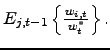 We
assume that remittances represent an altruistic compensation
mechanism between foreign workers residing in Home and Foreign.
Thus, in addition to the steady-state level of average remittances
We
assume that remittances represent an altruistic compensation
mechanism between foreign workers residing in Home and Foreign.
Thus, in addition to the steady-state level of average remittances
![]() , worker
, worker ![]() remits
an extra lump-sum amount
remits
an extra lump-sum amount ![]() if the forecast is
if the forecast is
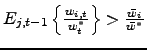 , so that
![]() . A relative wage
forecast above the steady-state ratio signals relative economic
hardship for household members residing in Foreign, and triggers
worker
. A relative wage
forecast above the steady-state ratio signals relative economic
hardship for household members residing in Foreign, and triggers
worker ![]() 's decision to remit the extra funds. For
symmetry, a relative wage forecast below the steady state results
in remittances equal to
's decision to remit the extra funds. For
symmetry, a relative wage forecast below the steady state results
in remittances equal to
![]()
Following Acosta et al. (2009), we also assume that immigrant
worker ![]() bases the relative wage forecast on a
noisy signal that is worker-specific:
bases the relative wage forecast on a
noisy signal that is worker-specific:
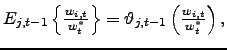 where
where
![]() is a random variable
drawn from a common uniform distribution
is a random variable
drawn from a common uniform distribution
![]() with support on the
interval
with support on the
interval
![$ \left[ 1-\Omega_{t} ^{f},1+\Omega_{t}^{f}\right] ,$](img268.gif) with
with
![]() . From this
specification, we have that
. From this
specification, we have that
![]() on
average, immigrant workers correctly predict the value of future
relative wages.
on
average, immigrant workers correctly predict the value of future
relative wages.
We define a threshold value of the forecast signal,
![]() , so that
, so that
![]() Remittances will be above their steady-state level,
Remittances will be above their steady-state level,
![]() every time remitter
every time remitter
![]() gets a random variable realization above
this threshold,
gets a random variable realization above
this threshold,
![]() This
property implies a decreasing monotonic relationship between the
threshold realization and the actual wage ratio at the time
remittances are received:
This
property implies a decreasing monotonic relationship between the
threshold realization and the actual wage ratio at the time
remittances are received:
![]() where
where
![]()
The proportion of immigrant workers that send the extra lump-sum
amount of remittances every period is given by:
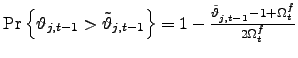 . This establishes a decreasing monotonic relationship between
average remittances and the threshold value of the forecast signal,
so that
. This establishes a decreasing monotonic relationship between
average remittances and the threshold value of the forecast signal,
so that
![]() where
where
![]() The presence of
a continuum of immigrant workers guarantees the differentiability
of
The presence of
a continuum of immigrant workers guarantees the differentiability
of ![]() . Finally, model symmetry guarantees
a stationary equilibrium where
. Finally, model symmetry guarantees
a stationary equilibrium where
![]() In essence, the model
with heterogeneous remitters presented in this appendix is
isomorphic to the one considered in the paper, in which identical
immigrant workers send average remittances equal to
In essence, the model
with heterogeneous remitters presented in this appendix is
isomorphic to the one considered in the paper, in which identical
immigrant workers send average remittances equal to ![]()
Using the equations above, we can express remittances per worker
as an increasing function of relative wages for any given value of
![]() , so that
, so that
![]() with
with
![]() . Thus, we
write average remittances as illustrated in equation (21) in the paper:
. Thus, we
write average remittances as illustrated in equation (21) in the paper:
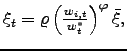 where
where ![]()
![]() is the
elasticity of average remittances with respect to relative wages.
The elasticity
is the
elasticity of average remittances with respect to relative wages.
The elasticity ![]() depends on the amount of
lump-sum funds,
depends on the amount of
lump-sum funds, ![]() and thus characterizes the
thrust of the altruistic motive. It also varies with
and thus characterizes the
thrust of the altruistic motive. It also varies with
![]() which we interpret as a
measure of uncertainty. This link between
which we interpret as a
measure of uncertainty. This link between ![]() and
and
![]() is underpinned by the second
differential,
is underpinned by the second
differential,
![]() . The intuition is that average remittances are less sensitive to
changes in the wage ratio under higher uncertainty about the
reliability of the forecast
. The intuition is that average remittances are less sensitive to
changes in the wage ratio under higher uncertainty about the
reliability of the forecast
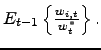
Table 1: Calibrated Parameters
| Parameter | Description | Value |
|---|---|---|
| Β | Discount factor | 0.99 |
| δ | Depreciation rate of capital | 0.025 |
| ω(ω*) | Home bias in Home (Foreign) | 0.85 (0.75) |
| α | Capital share in production | 0.33 |
| δl | Return probability of immigrant labor | 0.07 |
| s | Share of skilled workers in home labor force | 0.92 |
Table 2: Summary of the Prior and Posterior Distributions of the Estimated Parameters
| Description | Prior distribution: Name | Prior distribution: Density | Prior distribution: Mean | Prior distribution: Std Dev | Posterior distribution: Sd (Hess) | Posterior distribution: Mode | Posterior distribution: Mean | Posterior distribution: 5% | Posterior distribution: 95%% |
|---|---|---|---|---|---|---|---|---|---|
| Share of unskilled labor in output | γ | Gamma | 0.055 | 0.01 | 0.0086 | 0.0674 | 0.0673 | 0.0532 | 0.0810 |
| Elast. of subst. (K, unskilled) | θ | Beta | 0.95 | 0.015 | 0.0180 | 0.9448 | 0.9404 | 0.9123 | 0.9697 |
| Elast. of subst. (K, skilled) | η | Beta | 0.85 | 0.015 | 0.0092 | 0.9095 | 0.9076 | 0.8928 | 0.9230 |
| Product. of native skilled | ζ | Gamma | 6.2 | 0.75 | 0.7753 | 7.4039 | 7.3981 | 6.1061 | 8.6482 |
| Sunk emigration cost | fe | Gamma | 3.8 | 0.35 | 0.2735 | 5.5893 | 5.5225 | 5.0775 | 5.9767 |
| Inverse elast. of labor supply | ψ | Gamma | 1 | 0.2 | 0.2472 | 1.7686 | 1.8691 | 1.4605 | 2.2670 |
| Elast. of subst., goods | μ | Gamma |
1.5 | 0.3 | 0.2632 | 2.3735 | 2.2917 | 1.7610 | 2.7061 |
| Elast. of remittances to wages | φ | Gamma | 0.99 | 0.1 | 0.0985 | 0.9746 | 0.9828 | 0.8199 | 1.1427 |
| Neutral tech. shock (H) | ρa | Beta | 0.75 | 0.1 | 0.0233 | 0.9505 | 0.9418 | 0.9051 | 0.9792 |
| Neutral tech. shock (F) | ρa* | Beta | 0.75 | 0.1 | 0.0424 | 0.9789 | 0.9341 | 0.8721 | 0.9938 |
| Discount factor shock (H) | ρb | Beta | 0.5 | 0.05 | 0.0387 | 0.6541 | 0.6562 | 0.5923 | 0.7202 |
| Invest. tech. shock (H) | ρi | Beta | 0.5 | 0.05 | 0.0270 | 0.7655 | 0.7482 | 0.7111 | 0.7902 |
| Discount factor shock (F) | ρb* | Beta | 0.5 | 0.05 | 0.0247 | 0.7565 | 0.7491 | 0.7159 | 0.7902 |
| Invest. tech. shock (F) | ρi* | Beta | 0.5 | 0.05 | 0.0374 | 0.6343 | 0.6371 | 0.5759 | 0.6985 |
| Border enforcement shock | ρf e | Beta | 0.75 | 0.1 | 0.0031 | 0.9958 | 0.9940 | 0.9896 | 0.9986 |
| Neutral tech. shock (H) | σa | Inv gamma | 0.01 | 2* | 0.0005 | 0.0065 | 0.0066 | 0.0058 | 0.0074 |
| Neutral tech. shock (F) | σa* | Inv gamma | 0.01 | 2* | 0.0013 | 0.0176 | 0.0178 | 0.0156 | 0.0199 |
| Discount factor shock (H) | σb | Inv gamma | 0.01 | 2* | 0.0031 | 0.0390 | 0.0402 | 0.0352 | 0.0454 |
| Invest. tech. shock (H) | σi | Inv gamma | 0.01 | 2* | 0.0025 | 0.0316 | 0.0327 | 0.0285 | 0.0367 |
| Discount factor shock (F) | σb* | Inv gamma | 0.01 | 2* | 0.0033 | 0.0282 | 0.0312 | 0.0258 | 0.0365 |
| Invest. tech. shock (F) | σi* | Inv gamma | 0.01 | 2* | 0.0023 | 0.0172 | 0.0188 | 0.0150 | 0.0225 |
| Border enforcement shock | σf e | Inv gamma | 0.01 | 2* | 0.0037 | 0.0510 | 0.0515 | 0.0454 | 0.0574 |
Notes: For the Inverted gamma function the degrees of freedom are indicated. Results are based on 500,000 simulations of the Metropolis-Hastings algorithm.
Table 3: Unconditional Moments for Mexico and the U.S.
| Variable (growth) | St. dev. | Autocorr. | Corr with GDPUS/(Q*GDPMex) | Corr with GDPUS | Corr with Q*GDPMex |
|---|---|---|---|---|---|
| Apprehensions | 12.52 | -0.07 | 0.13 | 0.03 | -0.13 |
| Remittances | 7.07 | -0.08 | 0.61 | 0.09 | -0.61 |
| Border enforcement | 5.18 | 0.46 | -0.04 | 0.05 | 0.01 |
Note: Variables were transformed in delta ln (and thus expressed in growth rates). The sample period for border enforcement and apprehensions is 1980:2 to 2004:3. For workers's remittances, the sample period is 1995:2 to 2006:3.
Table 4: Unconditional Moments for the Estimated Benchmark Model
| Variable (growth) | St. dev. | Autocorr. | Corr with GDPh/(Q*GDPf) | Corr with GDPh | Corr with Q*GDPf |
|---|---|---|---|---|---|
| Migration flows | 17.57 (13.37/22.27) |
-0.15 (-0.18/-0.10) |
0.27 |
-0.03 (-0.10/0.02) |
-0.32 (-0.36/-0.27) |
| Remittances | 1.83 (1.61/2.05) |
0.06 (-0.02/0.18) |
0.57 (0.43/0.72) |
0.42 (0.31/0.52) |
-0.22 (-0.42/-0.06) |
| Border enforcement | 5.18 (4.67/5.70) |
0.00 (-0.01/0.00) |
-0.04 (-0.05/-0.02) |
0.01 (0.00/0.01) |
0.05 (0.03/0.06) |
Note: We report the median from the simulated distribution of moments using the samples generated with parameters draws of the posterior distribution. The 5th and 95th percentiles are included. See additional details in Table 3.
Table 5: Counterfactual Moments with Different Levels of Border Enforcement
| Variable (growth) | Corr with GDPh/(Q*GDPf) | Corr with GDPh | Corr with Q*GDPf |
|---|---|---|---|
| fe=6: Apprehensions | 0.27 | 0.01 | -0.30 |
| fe=6: Remittances | 0.52 | 0.35 | -0.22 |
| fe=6: Border enforcement | -0.02 | 0.01 | 0.03 |
| fe=1: Apprehensions | 0.51 | 0.29 | -0.30 |
| fe=1: Remittances | 0.50 | 0.51 | -0.09 |
| fe=1: Border enforcement | -0.01 | 0.00 | 0.02 |
Note: We simulate the model using the posterior median of the estimated parameters, with the exception of the parameter characterizing the steady-state level of border enforcement (fe). See additional details in Table 3.
Table 6: Welfare Gain/Loss of Switching From fe=5.52
| Low share of native unskilled: noshocks | Low share of native unskilled: shocks | High share of native unskilled: noshocks | High share of native unskilled: shocks | |
|---|---|---|---|---|
| To fe=1 | +3.63% | +4.36% | +1.01% | 0.06% |
| To fe=6 | -0.52% | -0.67% | 0% | +0.58% |
Note: The table shows the welfare gain/loss expressed as a percentage of the steady-state stream of expected consumption in Home when switching from the estimated sunk cost parameter (fe=5.52) to either a low sunk cost (fe=1) or high sunk cost (fe=6) regime. We consider two alternative scenarios, in which the share of the native unskilled labor is either low (8 percent) or high (25 percent).
Figure 1. Border Apprehensions and the U.S.-Mexico GDP Ratio
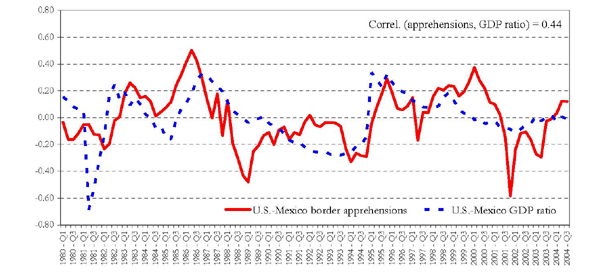
Note: Border apprehensions and the GDP ratio are seasonally adjusted and de-trended with a cubic trand. The U.S.-Mexico GDP ration is computed as the ration between (1) the U.S> real GDP (2) the real Mexican GDP multiplied by teh bilateral real exchange rate.
Figure 2. Remmittances, the U.S.-Mexico GDP Ratio, and the U.S.-Mexico Unskilled Wage Ratio
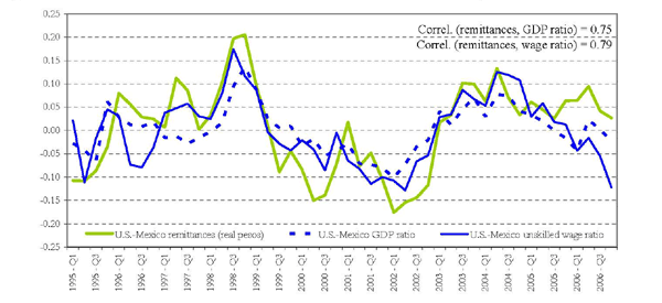
Note: Remittances are expressed in Mexican pesos at constant prices. The U.S.-Mexico wage ratio is computed as the ratio between (1) the U.S. real unskilled wage and (2) the maquiladora real wage in Mexico multiplied by the bilateral real exchange rate. See additional notes to Figure 1.
Figure 3. Data and Predicted Values from the Model
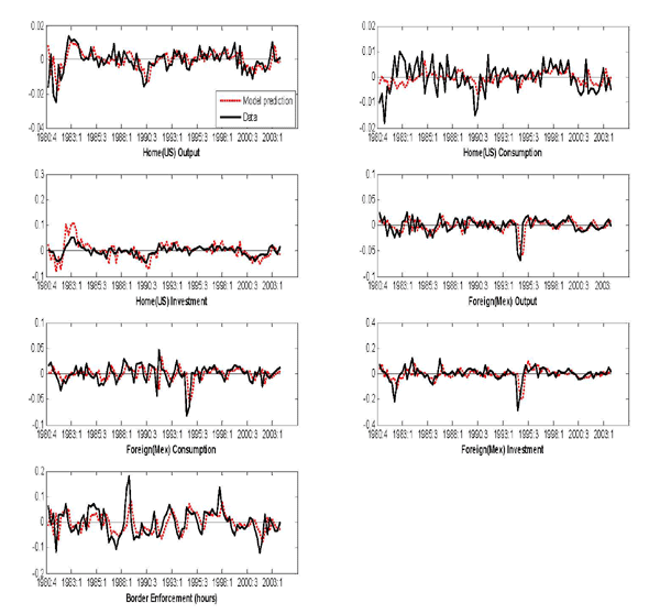
Note: Data (solid line) and benchmark model�s Kalman filtered one-sided predicted values (dashed line). Variables are transformed in Δln, and thus measured in growth rates.
Figure 4. Autocovariance Functions
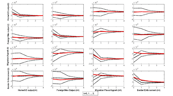
Note: The vector auto-covariance function is computed by estimating an unrestricted VAR (1) model with an uninformative prior for the variables plotted. The thin solid line refers to the median vector auto-covariance function, and the dotted lines represent the 2.5 and 97.5 percentiles. The thick solid line refers to the actual data.
Figure 5. Impulse Response to an Increase in Border Enforcement
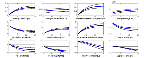
Note: The solid line is the median impulse response to a border enforcement shock (one standard deviation). The dashed lines are the 10 and 90 percent posterior intervals. We express the impulse responses as level deviations from steady-state.
Figure 6. Impulse Responses to a Positive Neutral Technology Shock in Home, Low vs. High Sunk Emigration Cost
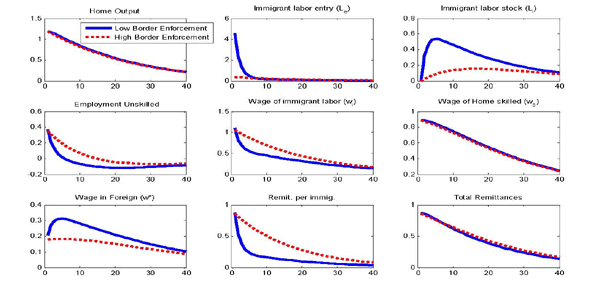
Note: Impulse response to a positive neutral technology shock at the median of the estimated parameters with the exception of fe (which we set as fe =1 for low border enforcement, and fe =6 for high border enforcement). For model comparisons, we express the impulse responses as percentage deviations from steady-state. In each case, we plot the impulse responses to a 1% increase in neutral technology in Home.
Figure 7. Impulse Responses to a Positive Neutral Technology Shock in Home, Financial Autarky vs. Integration
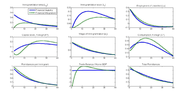
Note: Impulse responses to a positive neutral technology shock at the median of the estimated parameters, expressed as percentage deviations from steady-state.
Figure 8. Forecast Error Variance Decompositions
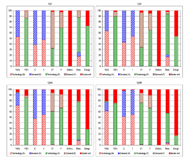
Note: Forecast variance decomposition at the posterior mode. We include the seven observables in the measurement set, remittances and migration flows. Forecast horizons: Q1, Q4, Q16 and Q40. Technology shocks include both neutral and investment-specific shocks.
Figure 9. Historical Decomposition
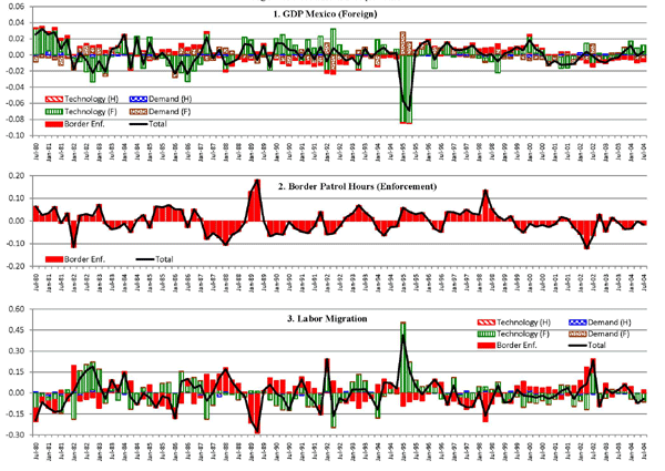
Technical Appendix and Additional Results
In this appendix, we present the model derivation and provide technical details on the Bayesian estimation. We include: (A) The derivation of the asymmetric steady state of the model; (B) Description of the data and its sources, the estimation methodology, and the Kalman smoothing procedure; (C) Sensitivity analysis, as we estimate the benchmark model with linearly detrended data (rather than the data in deviations from a cubic trend), and also the alternative model with international bond trading; (D) We plot the prior and posterior densities of the parameters of the benchmark model; the median impulse responses to each of the model shocks, including the 10 and 90 percent posterior intervals; and the Markov Chain Monte Carlo (MCMC) univariate and multivariate convergence diagnostics.
A Derivation of the Asymmetric Steady State
In this appendix, variables without time subscripts represent
steady-state values. We calibrate the steady-state values of labor
![]() ,
,
![]() and
and
![]() , and compute the corresponding
weights on the disutility from labor
, and compute the corresponding
weights on the disutility from labor ![]() ,
,
![]() , and
, and
![]() . Using the Euler equations, we
obtain the rental rate of capital net of depreciation as
. Using the Euler equations, we
obtain the rental rate of capital net of depreciation as
![]() 30 From the rule of motion of the stock
of capital we get
30 From the rule of motion of the stock
of capital we get
![]() and
and
![]() . From the rule of
motion of the stock of immigrant labor it follows that
. From the rule of
motion of the stock of immigrant labor it follows that
![]() .
.
The Foreign Economy Using the Cobb-Douglas production function
 , it follows that:
 |
 |
(1) |
 |
(2) | |
 |
(3) | |
 |
 |
(4) |
The Home Economy We solve the steady state for Home numerically using a system of
eight non-linear equations (5, 6, 9-18 below) in eight
unknowns (
![]() ,
, ![]() ,
,
![]() ,
,
![]() ,
, ![]() ,
,
![]() ,
, ![]() ,
, ![]() ), as follows:
), as follows:
Equations 1-2: In steady state, output and the marginal product of capital are:
 |
![$\displaystyle =\gamma^{\frac{1}{\theta}}\left( L_{i}+L_{u}\right) ^{\frac{\theta-1} {\theta}}+\left( 1-\gamma\right) ^{\frac{1}{\theta}}\left[ \lambda ^{\frac{1}{\eta}}K^{\frac{\eta-1}{\eta}}+(1-\lambda)^{\frac{1}{\eta}}\left( \zeta L_{s}\right) ^{\frac{\eta-1}{\eta}}\right] ^{\frac{\eta}{\eta-1} \frac{\theta-1}{\theta}},$](imga31.gif) |
(5) |
![$\displaystyle =p_{h}\left( 1-\gamma\right) ^{\frac{1}{\theta} }\lambda^{\frac{1}{\eta}}\left( \widetilde{Y}_{h}\right) ^{\frac{1}{\theta} }\left[ \lambda^{\frac{1}{\eta}}K^{\frac{\eta-1}{\eta}}+(1-\lambda)^{\frac {1}{\eta}}\left( \zeta L_{s}\right) ^{\frac{\eta-1}{\eta}}\right] ^{\frac{\theta-\eta}{\left( \eta-1\right) \theta}}K^{-\frac{1}{\eta}}.$](imga33.gif) |
(6) |
Equation 3: Using the steady-state expression for the net
present value of the gains from emigration,
![]() , we obtain:
, we obtain:
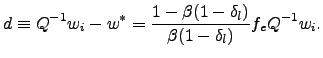 |
(7) |
As a result, the steady-state ratio between the immigrant wage in Home and the wage in the country of origin, expressed in units of the home consumption basket, is:
![$\displaystyle \Omega\equiv\frac{w_{i}}{w^{\ast}Q}=\left[ 1-\frac{1-\beta(1-\delta_{l} )}{\beta(1-\delta_{l})}f_{e}\right] ^{-1}.$](imga36.gif) |
(8) |
Note that when ![]() , it follows that
, it follows that ![]() . In other words, when the sunk emigration cost is
zero, labor migration will take place up the the point at which, in
equilibrium, the immigrant wage is equal to the wage in the country
of origin.
. In other words, when the sunk emigration cost is
zero, labor migration will take place up the the point at which, in
equilibrium, the immigrant wage is equal to the wage in the country
of origin.
Next, we insert
 and
and
 into equation 8 to
obtain:
into equation 8 to
obtain:
 |
(9) |
Equation 4: The balanced current account condition implies:
 |
(10) |
in which we use:
![$\displaystyle =\frac{L^{\ast}}{L^{\ast}-L_{i}}\left[ Y^{\ast}-\delta K^{\ast }-f_{e}w_{i}\frac{L_{e}}{Q}\right] ,$](imga44.gif) |
(11) | |
![$\displaystyle =\left[ \omega^{\ast\frac{1}{\mu}}\left( \widetilde{Y} _{f}-Y_{f}\right) ^{\frac{\mu-1}{\mu}}+\left( 1-\omega^{\ast}\right) ^{\frac{1}{\mu}}\left( Y_{h}^{\ast}\right) ^{\frac{\mu-1}{\mu}}\right] ^{\frac{\mu}{\mu-1}},$](imga46.gif) |
(12) | |
 |
(13) | |
 |
(14) |
Equations 5-6: We write the demand ratios for the two intermediate goods in each economy as:
 |
 |
(15) |
 |
 |
(16) |
Equations 7-8: The price indexes for the composite good of each country are:
| (17) | ||
 |
(18) |
Next we use the steady-state values for
![]() ,
, ![]() ,
,
![]() ,
,
![]() ,
, ![]() ,
,
![]() ,
, ![]() , and
, and
![]() computed above to obtain solutions for the
rest of the variables. The equations above provide the solutions
for
computed above to obtain solutions for the
rest of the variables. The equations above provide the solutions
for
![]() ,
, ![]() and
and
![]() in Home, and for
in Home, and for
![]() ,
, ![]() ,
,
![]() ,
, ![]() ,
, ![]() in Foreign. The remaining variables for Home
are:
in Foreign. The remaining variables for Home
are:
| (19) | ||
![$\displaystyle =\left[ \omega^{\frac{1}{\mu}}\left( Y_{h}\right) ^{\frac{\mu-1}{\mu }}+(1-\omega)^{\frac{1}{\mu}}\left( Y_{f}\right) ^{\frac{\mu-1}{\mu} }\right] ^{\frac{\mu}{\mu-1}},$](imga78.gif) |
(20) | |
![$\displaystyle =p_{h}\left( 1-\gamma\right) ^{\frac{1}{\theta}}(1-\lambda )^{\frac{1}{\eta}}\left( \tilde{Y}_{h}\right) ^{\frac{1}{\theta}}\left[ \lambda^{\frac{1}{\eta}}\left( K_{t}\right) ^{\frac{\eta-1}{\eta} }+(1-\lambda)^{\frac{1}{\eta}}\left( \zeta L_{s,t}\right) ^{\frac{\eta -1}{\eta}}\right] ^{\frac{\theta-\eta}{\left( \eta-1\right) \theta}}\left( L_{s}\right) ^{-\frac{1}{\eta}},$](imga80.gif) |
(21) | |
![$\displaystyle =\left[ s+(1-s)\frac{(1-\phi)}{\phi}\right] ^{-1}\left( Y-\delta K-\frac{L_{i}}{L^{\ast}}C^{\ast}Q\right) ,$](imga82.gif) |
(22) | |
 |
(23) |
The remaining variables for Foreign are
![]() and
and
![]() .
Finally, the weights on the disutility from labor are
.
Finally, the weights on the disutility from labor are
![]() ,
,
![]() and
and
![]() .
.
Financial Integration In the extended model with international bond trading described
above, we use
![]() ,
,
![]() and
and
![]() in Home to obtain
in Home to obtain
![]() and
and
![]() Similarly for Foreign,
using that
Similarly for Foreign,
using that
![]() ,
,
![]() and
and
![]() it also follows that
it also follows that
![]() and
and
![]()
Finally, the balanced current account condition (10) is replaced by the following expression for the balance of international payments in steady state:
 |
(24) |
The steady-state solutions for all other variables are the same as under financial autarky.
B The Bayesian Estimation
B.1 Data Sources
Macroeconomic data on real output, consumption and investment is provided by the Bureau of Economic Analysis (for the U.S.) and INEGI (for Mexico) through Haver Analytics. Data on apprehensions at the U.S.-Mexico border and the number of hours spent by the U.S. Border Patrol on policing the border is provided by the U.S. Immigration and Naturalization Service, and made available on Gordon Hanson's website ("border linewatch apprehensions" and "border linewatch enforcement hours"). Data on workers' remittances in nominal U.S. dollars is provided by the Bank of Mexico through Haver Analytics. We convert remittances in real dollars using the U.S. CPI index, and then in real Mexican pesos using the U.S.-Mexico bilateral real exchange (obtained from the IMF's International Financial Statistics). The U.S. Census Bureau's Current Population Survey (CPS) is the source for hours worked and hourly wages (in nominal dollars) for the U.S. skilled and unskilled workers. We used monthly data for total hours worked in the last week of every month, weekly earnings before deductions, and earnings weights by educational attainment. Data on hours worked and hourly wages for Mexico's maquiladora sector (in nominal pesos) is provided by INEGI; we compute the hourly wage in nominal pesos using the monthly series on total remunerations, total number of workers, and hours per worker. In order to compute the U.S. unskilled-Mexico maquiladora wage ratio, we convert the maquiladora wage in U.S. dollars using the nominal exchange rate. We seasonally adjust the data with the X-12 ARIMA method of the U.S. Census Bureau.
B.2 Estimation Methodology
In this section we briefly explain the estimation approach used
in this paper. A more detailed description of the method can be
found in Lubik and Schorfheide (2005), Justiniano and Preston
(2010), and Schorfheide (2000) among others. Let's define
![]() as the parameter space of the DSGE
model, and
as the parameter space of the DSGE
model, and
![]() as
the data series used in the estimation. From their joint
probability distribution
as
the data series used in the estimation. From their joint
probability distribution
![]() , we can derive a
relationship between the marginal
, we can derive a
relationship between the marginal ![]() and
the conditional distribution
and
the conditional distribution
![]() which is known as the
Bayes theorem:
which is known as the
Bayes theorem:
![]() The
method updates the a priori distribution using the
likelihood contained in the data to obtain the conditional
posterior distribution of the structural parameters. The resulting
posterior density
The
method updates the a priori distribution using the
likelihood contained in the data to obtain the conditional
posterior distribution of the structural parameters. The resulting
posterior density
![]() is used to draw
statistical inference on the parameter space
is used to draw
statistical inference on the parameter space ![]() . Combining the state-form representation implied by
the solution for the linear rational expectation model and the
Kalman filter, we can compute the likelihood function. The
likelihood and the prior permit a computation of the posterior that
can be used as the starting value of the random walk version of the
Metropolis-Hastings (MH) algorithm, which is a Monte Carlo method
used to generate draws from the posterior distribution of the
parameters. In this case, the results reported are based on 500,000
draws following this algorithm. We choose a normal jump
distribution with covariance matrix equal to the Hessian of the
posterior density evaluated at the maximum. The scale factor is
chosen in order to deliver an acceptance rate between 30 and 45
percent depending on the run of the algorithm. Measures of
uncertainty follow from the percentiles of the draws.
. Combining the state-form representation implied by
the solution for the linear rational expectation model and the
Kalman filter, we can compute the likelihood function. The
likelihood and the prior permit a computation of the posterior that
can be used as the starting value of the random walk version of the
Metropolis-Hastings (MH) algorithm, which is a Monte Carlo method
used to generate draws from the posterior distribution of the
parameters. In this case, the results reported are based on 500,000
draws following this algorithm. We choose a normal jump
distribution with covariance matrix equal to the Hessian of the
posterior density evaluated at the maximum. The scale factor is
chosen in order to deliver an acceptance rate between 30 and 45
percent depending on the run of the algorithm. Measures of
uncertainty follow from the percentiles of the draws.
B.3 Smoothing
The DSGE model can be written in a state-space representation as
![]() and
and
![]() , in which
, in which
![]() is the vector of unobserved
variables at date
is the vector of unobserved
variables at date ![]() , and
, and ![]() is the vector of observables
is the vector of observables![]() shocks
shocks
![]() and
and ![]() are
uncorrelated, normally distributed, white noise vectors. The first
expression is the state equation and the second the is the
observed equation.
are
uncorrelated, normally distributed, white noise vectors. The first
expression is the state equation and the second the is the
observed equation.
Smoothing involves the estimation of
![]() conditional on the full data set
conditional on the full data set ![]() used in the
estimation. The smoothed estimates are denoted
used in the
estimation. The smoothed estimates are denoted
![]() and, as
shown in Bauer et al. (2003), can be written as:
and, as
shown in Bauer et al. (2003), can be written as:
| (25) |
in which
![]() is the mean squared forecasting error associated with the
projection of
is the mean squared forecasting error associated with the
projection of ![]() on
on ![]() and a
constant, projection which is denoted as
and a
constant, projection which is denoted as
![]() .
Using the Kalman Filter to calculate
.
Using the Kalman Filter to calculate
![]()
![]()
![]() and
and
![]() the sequence of smooth estimates
the sequence of smooth estimates
![]() is
determined from equation (25).
is
determined from equation (25).
C Additional Results and Sensitivity Analysis
For robustness, in Table A1 we report the estimation results obtained for the benchmark model with financial autarky using linearly detrended data. (In contrast, Table 2 in the main paper uses data in percent deviations from a cubic trend.) Table A2 reports the estimation results for the model with financial integration, using the data in deviations from a cubic trend. In Figure A1, we show the prior (grey line), posterior density (black line) and mode from the numerical optimization of the posterior kernel (dashed line) for the benchmark model. Figure A2 reports impulse responses to all shocks (neutral technology, demand and investment in either Home or Foreign). We depict the median response (solid lines) to a one standard deviation of the shocks, along with the 10 and 90 percent posterior intervals (dashed lines).
D Convergence Diagnostics
We monitor the convergence of iterative simulations with the methods described in Brooks and Gelman (1998).
General Univariate Diagnostics The empirical 80 percent interval for any given parameter,
![]() , is taken from each individual chain
first. The interval is described by the 10 and 90 percent of the
, is taken from each individual chain
first. The interval is described by the 10 and 90 percent of the
![]() simulated draws. Then,
simulated draws. Then, ![]() within-sequence interval length estimates are constructed. Next, a
set of
within-sequence interval length estimates are constructed. Next, a
set of ![]() observations, generated from all chains,
is also used to calculate the 80% interval, and a total-sequence
interval length estimate is obtained, so that
observations, generated from all chains,
is also used to calculate the 80% interval, and a total-sequence
interval length estimate is obtained, so that
![]() can be evaluated
can be evaluated![]() Convergence is approached when the
numerator and denominator coincide (i.e.
Convergence is approached when the
numerator and denominator coincide (i.e.
![]()
It is also possible to compute non interval-based alternatives,
which we report for robustness. The numerator and denominator in
the expression above is replaced by an empirical estimate of the
central ![]() order moments calculated from all
sequences together, and the mean
order moments calculated from all
sequences together, and the mean ![]() order moment
is calculated from each individual sequence, so as to define for
every
order moment
is calculated from each individual sequence, so as to define for
every ![]() :
:
 In Figure A3, we plot the numerator and denominator from measures
of
In Figure A3, we plot the numerator and denominator from measures
of
![]() for each of the parameters estimated
for each of the parameters estimated![]() The scale
used for drawing the initial value of the MH chain is twice that of
the jumping distribution in the MH algorithm. As it is observed,
convergence is achieved before 100,000 iterations (we use five
parallel chains).
The scale
used for drawing the initial value of the MH chain is twice that of
the jumping distribution in the MH algorithm. As it is observed,
convergence is achieved before 100,000 iterations (we use five
parallel chains).
Multivariate extensions In this case, we redefine ![]() as a a
vector parameter based upon observations
as a a
vector parameter based upon observations
![]() denoting the
denoting the ![]() element of the parameter vector in chain
element of the parameter vector in chain ![]() at time
at time ![]() The direct analogue of univariate
approach in higher dimensions is to estimate the posterior
variance-covariance matrix as:
The direct analogue of univariate
approach in higher dimensions is to estimate the posterior
variance-covariance matrix as:
![]() where
where
![]() and
and
![]() It is possible to summarize the distance between
It is possible to summarize the distance between ![]() and
and ![]() with a scalar measure that
should approach 1 (from above) as convergence is achieved, given
suitably overdispersed starting points. We can monitor both
with a scalar measure that
should approach 1 (from above) as convergence is achieved, given
suitably overdispersed starting points. We can monitor both
![]() and
and ![]() determining
convergence when any rotationally invariant distance measure
between the two matrices indicates that they are sufficiently
close. In Figure A4, we report measures of this aggregate.31
Convergence is achieved before 100,000 iterations.32
determining
convergence when any rotationally invariant distance measure
between the two matrices indicates that they are sufficiently
close. In Figure A4, we report measures of this aggregate.31
Convergence is achieved before 100,000 iterations.32
References
Bauer, A. , Haltom, N., and Rubio-Ramírez, J. (2003). "Using the Kalman Filter to Smooth the Shocks of a Dynamic Stochastic General Equilibrium Model," Federal Reserve Bank of Atlanta, Working Paper 2003-32.
Brooks, S., Gelman, A. (1998). "General Methods for Monitoring Convergence of Iterative Simulations," Journal of Computational and Graphical Statistics 7(4), 434-455.
INEGI (El Instituto Nacional de Estadística y Geografía, Mexico, 2008). Banco de Información Económica, http://dgcnesyp.inegi.org.mx/cgi-win/bdieintsi.exe
Justiniano, A. and Preston, B. (2010). "Monetary Policy and Uncertainty in an Empirical Small Open Economy Model," Journal of Applied Econometrics, 25(1).
Lubik, T. and Schorfheide, F. (2005). "A Bayesian Look at New Open Economy Macroeconomics," NBER Macroeconomics Annual, 313-366.
Schorfheide, F. (2000). "Loss Function Based Evaluation of DSGE Models," Journal of Applied Econometrics 15(6), 645-670.
U.S. Census Bureau (2007). Current Population Survey (CPS), Annual Social and Economic Supplement.
Table A1: Summary Statistics for the Benchmark Model with Financial Autarky
| Description | Prior distribution: Name | Prior distribution: Density | Prior distribution: Mean | Prior distribution: Std Dev | Posterior distribution: Sd (Hess) | Posterior distribution: Mode | Posterior distribution: Mean | Posterior distribution: 5% | Posterior distribution: 95%% |
|---|---|---|---|---|---|---|---|---|---|
| Share of unskilled labor in output | γ | Gamma | 0.055 | 0.01 | 0.0073 | 0.0463 | 0.0548 | 0.0435 | 0.0667 |
| Elast. of subst. (K, unskilled) | θ | Beta | 0.95 | 0.015 | 0.0160 | 0.9584 | 0.9438 | 0.9194 | 0.9711 |
| Elast. of subst. (K, skilled) | η | Beta | 0.85 | 0.015 | 0.0095 | 0.8894 | 0.9051 | 0.8894 | 0.9204 |
| Product. of native skilled | ζ | Gamma | 6.2 | 0.75 | 0.7442 | 6.2091 | 6.7725 | 5.6067 | 8.0518 |
| Sunk emigration cost | fe | Gamma | 3.8 | 0.35 | 0.2419 | 3.37831 | 6.0988 | 5.7650 | 6.4663 |
| Inverse elast. of labor supply | ψ | Gamma | 1 | 0.2 | 0.2415 | 1.1223 | 2.1114 | 1.7127 | 2.5006 |
| Elast. of subst., goods | μ | Gamma |
1.5 | 0.3 | 0.1819 | 1.5924 | 1.9022 | 1.6060 | 2.1894 |
| Elast. of remittances to wages | φ | Gamma | 0.99 | 0.1 | 0.1005 | 0.9864 | 0.9860 | 0.8194 | 1.1454 |
| Neutral tech. shock (H) | ρa | Beta | 0.75 | 0.1 | 0.0205 | 0.9837 | 0.9177 | 0.9056 | 0.9719 |
| Neutral tech. shock (F) | ρa* | Beta | 0.75 | 0.1 | 0.0271 | 0.9482 | 0.9354 | 0.8937 | 0.9808 |
| Discount factor shock (H) | ρb | Beta | 0.5 | 0.05 | 0.0310 | 0.6873 | 0.7118 | 0.6596 | 0.7613 |
| Invest. tech. shock (H) | ρi | Beta | 0.5 | 0.05 | 0.0253 | 0.6871 | 0.7536 | 0.7183 | 0.7902 |
| Discount factor shock (F) | ρb* | Beta | 0.5 | 0.05 | 0.0198 | 0.6280 | 0.7637 | 0.7369 | 0.7902 |
| Invest. tech. shock (F) | ρi* | Beta | 0.5 | 0.05 | 0.0043 | 0.7902 | 0.7800 | 0.7734 | 0.7855 |
| Border enforcement shock | ρf e | Beta | 0.75 | 0.1 | 0.0038 | 0.9807 | 0.9919 | 0.9863 | 0.9978 |
| Neutral tech. shock (H) | σa | Inv gamma | 0.01 | 2* | 0.0004 | 0.0061 | 0.0065 | 0.0058 | 0.0072 |
| Neutral tech. shock (F) | σa* | Inv gamma | 0.01 | 2* | 0.0014 | 0.0177 | 0.0178 | 0.0155 | 0.0198 |
| Discount factor shock (H) | σb | Inv gamma | 0.01 | 2* | 0.0029 | 0.0446 | 0.0413 | 0.0364 | 0.0459 |
| Invest. tech. shock (H) | σi | Inv gamma | 0.01 | 2* | 0.0026 | 0.0379 | 0.0348 | 0.0306 | 0.0392 |
| Discount factor shock (F) | σb* | Inv gamma | 0.01 | 2* | 0.0043 | 0.0880 | 0.0456 | 0.0389 | 0.0530 |
| Invest. tech. shock (F) | σi* | Inv gamma | 0.01 | 2* | 0.0032 | 0.0536 | 0.0284 | 0.0229 | 0.0332 |
| Border enforcement shock | σf e | Inv gamma | 0.01 | 2* | 0.0041 | 0.0536 | 0.0553 | 0.0489 | 0.0621 |
Notes: For the Inverted gamma function the degrees of freedom are indicated.
Table A2: Summary Statistics for the Benchmark Model with Financial Integration Estimated with Cubic Detrended Data
| Description | Prior distribution: Name | Prior distribution: Density | Prior distribution: Mean | Prior distribution: Std Dev | Posterior distribution: Sd (Hess) | Posterior distribution: Mode | Posterior distribution: Mean | Posterior distribution: 5% | Posterior distribution: 95%% |
|---|---|---|---|---|---|---|---|---|---|
| Share of unskilled labor in output | γ | Gamma | 0.055 | 0.01 | 0.0094 | 0.0957 | 0.0960 | 0.0809 | 0.1109 |
| Elast. of subst. (K, unskilled) | θ | Beta | 0.95 | 0.015 | 0.0171 | 0.9456 | 0.9405 | 0.9138 | 0.9680 |
| Elast. of subst. (K, skilled) | η | Beta | 0.85 | 0.015 | 0.0107 | 0.8854 | 0.8864 | 0.8696 | 0.9042 |
| Product. of native skilled | ζ | Gamma | 6.2 | 0.75 | 0.5827 | 6.1874 | 5.9279 | 4.9515 | 6.8451 |
| Sunk emigration cost | fe | Gamma | 3.8 | 0.35 | 0.1625 | 6.4665 | 6.1006 | 5.8442 | 6.3897 |
| Inverse elast. of labor supply | ψ | Gamma | 1 | 0.2 | 0.1897 | 1.312 | 1.3295 | 1.0078 | 1.6277 |
| Elast. of subst., goods | μ | Gamma |
1.5 | 0.3 | 0.1100 | 1.8934 | 1.8185 | 1.6443 | 2.0006 |
| Elast. of remittances to wages | φ | Gamma | 0.99 | 0.1 | 0.0964 | 0.9608 | 0.9600 | 0.8003 | 1.109 |
| Neutral tech. shock (H) | ρa | Beta | 0.75 | 0.1 | 0.0255 | 0.9602 | 0.9432 | 0.9051 | 0.9853 |
| Neutral tech. shock (F) | ρa* | Beta | 0.75 | 0.1 | 0.0300 | 0.9815 | 0.9499 | 0.9042 | 0.9935 |
| Discount factor shock (H) | ρb | Beta | 0.5 | 0.05 | 0.0400 | 0.6006 | 0.6148 | 0.5482 | 0.6807 |
| Invest. tech. shock (H) | ρi | Beta | 0.5 | 0.05 | 0.0346 | 0.3757 | 0.3819 | 0.3230 | 0.4376 |
| Discount factor shock (F) | ρb* | Beta | 0.5 | 0.05 | 0.0203 | 0.7834 | 0.7603 | 0.7312 | 0.7902 |
| Invest. tech. shock (F) | ρi* | Beta | 0.5 | 0.05 | 0.0188 | 0.7816 | 0.7647 | 0.7386 | 0.7902 |
| Border enforcement shock | ρf e | Beta | 0.75 | 0.1 | 0.0018 | 0.9973 | 0.9960 | 0.9935 | 0.9991 |
| Neutral tech. shock (H) | σa | Inv gamma | 0.01 | 2* | 0.0005 | 0.0071 | 0.0073 | 0.0065 | 0.0082 |
| Neutral tech. shock (F) | σa* | Inv gamma | 0.01 | 2* | 0.0012 | 0.0178 | 0.0179 | 0.0159 | 0.0200 |
| Discount factor shock (H) | σb | Inv gamma | 0.01 | 2* | 0.0011 | 0.0116 | 0.0125 | 0.0107 | 0.0143 |
| Invest. tech. shock (H) | σi | Inv gamma | 0.01 | 2* | 0.0007 | 0.0078 | 0.0086 | 0.0074 | 0.0098 |
| Discount factor shock (F) | σb* | Inv gamma | 0.01 | 2* | 0.0021 | 0.0219 | 0.0238 | 0.0202 | 0.0270 |
| Invest. tech. shock (F) | σi* | Inv gamma | 0.01 | 2* | 0.0009 | 0.0095 | 0.0103 | 0.0088 | 0.0117 |
| Border enforcement shock | σf e | Inv gamma | 0.01 | 2* | 0.0038 | 0.0508 | 0.0520 | 0.0459 | 0.0582 |
Notes: For the Inverted gamma function the degrees of freedom are indicated.
Figure A1. Prior and Posterior Distributions
Figure A1 (Continuation). Prior and Posterior Distributions
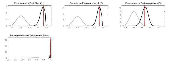
Note: Benchmark Model. Results based on 500,000 draws of the Metropolis algorithm. Gray line: prior. Black line: posterior. Vertical dashed line: posterior mode (from the numerical optimization of the posterior kernel).
Figure A2. Impulse Response Functions to the Model's Shocks - Neutral Technology Shock at Home
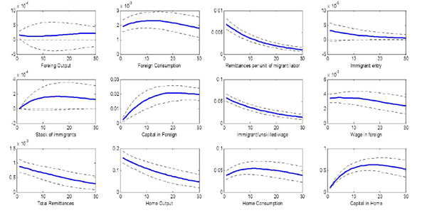
Figure A2 (continuation). Impulse Response Functions to the Model's Shocks - Neutral Technology Shock at Foreign
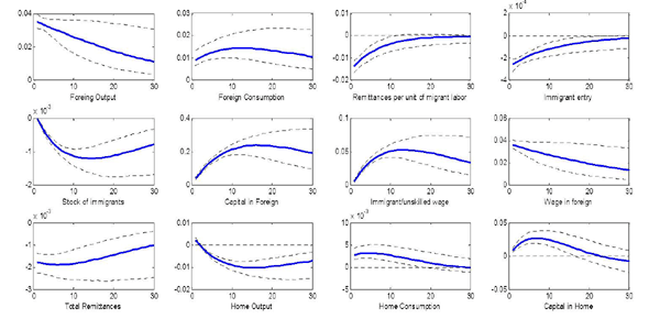
Figure A2 (continuation). Impulse Response Functions to the Model's Shocks - Demand Shock at Home

Figure A2 (continuation). Impulse Response Functions to the Model's Shocks - Investment Shock at Home
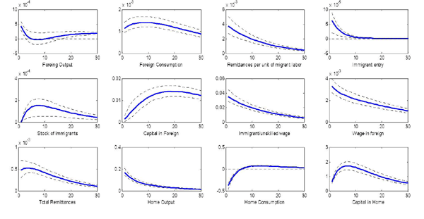
Figure A2 (continuation). Impulse Response Functions to the Model's Shocks - Demand Shock at Foreign
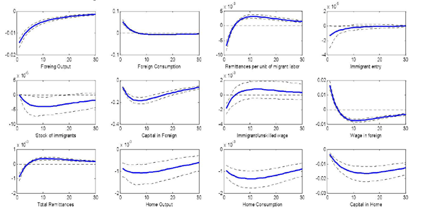
Figure A2 (continuation). Impulse Response Functions to the Model's Shocks - Investment Shock at Foreign
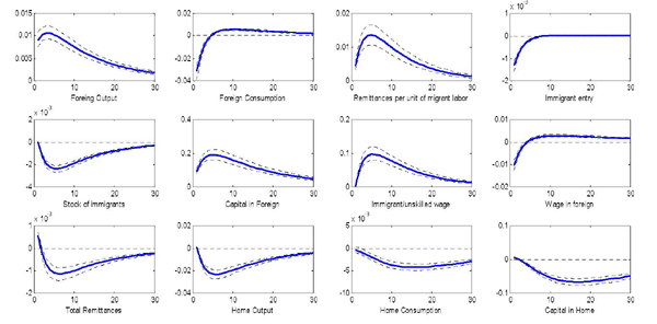
Note: The solid line is the median impulse response to one standard deviation of the shocks; the dotted lines are the 10 and 90 percent posterior intervals.
Figure A3. MCMC Univariate Convergence Diagnostics
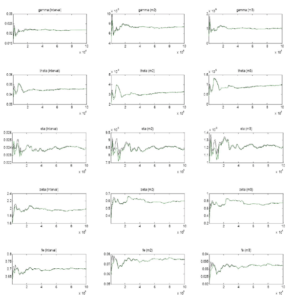
Figure A3 (Continuation). MCMC Univariate Convergence Diagnostics
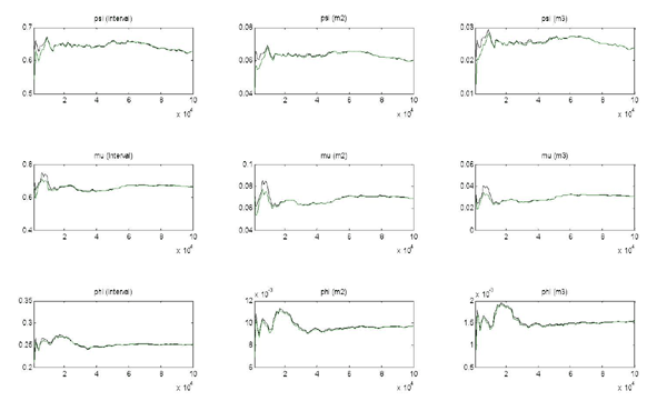
Note: Univariate convergence diagnostics (Brooks and Gelman, 1998). The first, second and third columns are the criteria based on the eighty percent interval, the second and third moments, respectively. Univariate diagnostics for the shocks are available upon request.
Figure A4. MCMC Multivariate Convergence Diagnostics
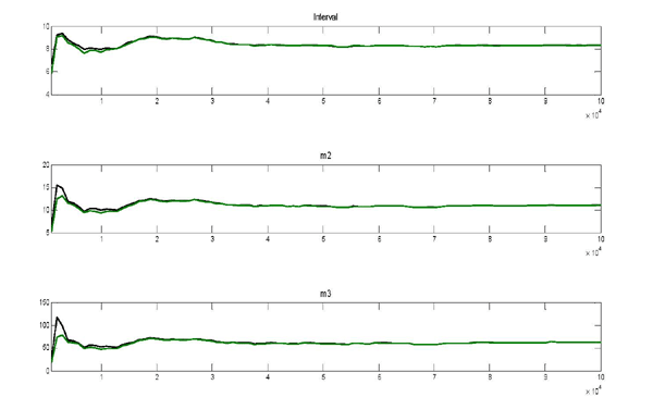
Note: Multivariate convergence diagnostics (Brooks and Gelman, 1998). The first, second and third graphs are the criteria based on the eighty percent interval, the second and third moments, respectively.
Footnotes
1. This paper is a significantly revised version of " Immigration and the Macroeconomy.'' We acknowledge Gustavo Canavire and Menbere Shiferaw for superb research assistance. We thank our discussants Mario Crucini and Bora Durdu, as well as James Anderson, Susanto Basu, Fabio Ghironi, Peter Ireland, Nobuhiro Kiyotaki, Giovanni Peri, Myriam Quispe-Agnoli, B. Ravikumar, Alessandro Rebucci, Pedro Silos, Nicole Simpson, and conference and seminar participants at the NBER Summer Institute (International Finance and Macroeconomics), Bank of Japan, Central Bank of the Philippines, FRB of Atlanta, Federal Reserve Board, FRB of Boston, Georgia Tech, Inter-American Development Bank and the University of Delaware, who provided helpful comments. Part of this project was developed while Andrei Zlate was visiting the FRB of Atlanta and the FRB of Boston, whose hospitality he gratefully acknowledges. The views in this paper are solely the responsibility of the authors and should not be interpreted as reflecting the views of the Federal Reserve Bank of Atlanta, the Board of Governors of the Federal Reserve System or of any other person associated with the Federal Reserve System. Return to text
2. Federal Reserve Bank of Atlanta, Research Department, 1000 Peachtree St N.E., Atlanta, GA, 30309, e-mail: [email protected]. Return to text
3. Board of Governors of the Federal Reserve System, Division of International Finance, 20th St and Constitution Ave NW, Washington, DC, 20551, e-mail: [email protected]. Return to text
4. For instance, the number of arrivals into the U.S. declined by almost 40 percent in the aftermath of the financial panic episode of 1907. Notable declines also were observed during the U.S. recessions of 1876-79, 1894 and 1922. At that time, there were fewer restrictions on the legal immigration from Europe, and most of the arrivals were properly documented (O'Rourke and Williamson, 1999). Therefore, the recorded flows of immigrant labor in the U.S. were closely related to the economic considerations modeled in this paper. Return to text
5. Similarly, Hanson and Spilimbergo (1999) find that a 10% relative decline in the Mexican real wage has been associated with a 6 to 8% increase in U.S. border apprehensions. Borger (2009) finds similar results using annual survey-based micro estimates of migration flows. Return to text
6. Examples for 2007 include Moldova (34.1%), Honduras (21.5%), Guyana (24.3%), Jordan (21.7%) and the Philippines (11.3%). See the World Bank's Global Development Finance (2009). Return to text
7. In 2008, total net international private capital flows to developing economies (which include 144 low income and lower/upper-middle income economies) reached $707 billion, less than the average of $793 billion of the previous four years. From this total, FDI accounted for $583 billion, while net portfolio equity and debt flows accounted for $124 billion. See World Bank (2009). Return to text
8. Rodríguez-Zamora (2008) shows that the recent increase in border enforcement resulted in less volatile migration inflows and outflows across the U.S.-Mexico border. After growing at double digit rates, remittances drastically fell in the aftermath of the U.S. financial crisis. Return to text
9. Due to the cross-country wage asymmetry, there is no labor migration from Home to Foreign. Return to text
10. Since home and foreign goods are imperfect substitutes, the demand for the foreign good is always positive, and a share of the foreign labor is always required for production in Foreign. Return to text
11. Absent other frictions, since wages in Home are always higher than in Foreign, the endogenous return decision rule is outside the scope of this model. The endogenous entry-exogenous exit formulation that we adopt follows the guidelines for firm entry and exit in Ghironi and Melitz (2005). Return to text
12. For simplicity, we assume that immigrant workers cannot invest their labor income in the home economy. Return to text
13. Variables marked with an upper bar denote steady state values. Return to text
14. Our mechanism of remittances is isomorphic to the one resulting from the framework with heterogeneous remitters described in Appendix B. Return to text
15. The parameter
![]() ensures that remittances in steady state are equal to the
difference between immigrant labor income and immigrant
consumption. Return to text
ensures that remittances in steady state are equal to the
difference between immigrant labor income and immigrant
consumption. Return to text
16. A more comprehensive discussion of the estimation, the data series used in the estimation, the Monte Carlo Markov Chain (MCMC) convergence diagnostics and additional results can be found in a separate technical appendix of this paper, available online. Return to text
17. The sources for all data series used in this paper are described in the technical appendix. Return to text
18.
![]()
![]() is the vector of observed variables, where
is the vector of observed variables, where
![]()
![]() We
use cubic detrending since the traditional HP filtering can result
in spurious cycles in the data that affect the estimates (see
Cogley and Nason, 1995, for details). For robustness, we also have
estimated the baseline model with linearly detrended data as in
Smets and Wouters (2003), and also the model with international
bond trading (and cubic-detrended data). The results, available in
the technical appendix, are very similar. Return to text
We
use cubic detrending since the traditional HP filtering can result
in spurious cycles in the data that affect the estimates (see
Cogley and Nason, 1995, for details). For robustness, we also have
estimated the baseline model with linearly detrended data as in
Smets and Wouters (2003), and also the model with international
bond trading (and cubic-detrended data). The results, available in
the technical appendix, are very similar. Return to text
19. For instance, using the information
that 35% of undocumented Mexican immigrants are still in the U.S.
four years after their arrival, we compute the quarterly exit rate
as
![]() , and thus
, and thus
![]() Return to text
Return to text
20. We take the weighted average of hourly earnings for the U.S. skilled labor (i.e. high school degree or more), as well as for the U.S. unskilled labor (i.e. without a high school degree) using data provided by the U.S. Census Bureau (2007). We divide the sample into four groups: (a) no high school degree; (b) completed high school; (c) some college or associate's degree; and (d) bachelor's degree or higher. Then we take the average of the respective earnings weighted by their share in the total population. Return to text
21. These are conservative estimates. Remittances tend to be underreported, particularly between neighboring countries. Return to text
22. For the first two variables, the sample period is 1980:2 to 2004:3. The sample period for remittances is 1995:2 to 2006:3. Return to text
23. We draw 3,000 parameter combinations from the posterior distribution and simulate 3,000 artificial data sets (of the same length as the ones in the data) to estimate vector autocovariance functions using the same VAR specification applied on the actual U.S./Mexico data. Return to text
24. Notice that in the previous section we calculated the median value of a set of moments generated with a large set of parameter draws from the posterior distribution. In this counterfactual scenario, we calculate moments by using just the median parameter values from the posterior distribution. The results should be close, but not necessarily the same. Return to text
25. The impulse response of the estimated model (median and percentiles) for all shocks are reported in a separated technical appendix available online. Return to text
26. The first-order approximation to the unconditional mean of endogenous variables coincides with their non-stochastic steady-state values. Return to text
27. Notice that this welfare gain holds even under the assumption that natives unskilled and immigrants are perfect substitutes as in Borjas et al. (2008). If some degree of complementarity exists (See for instance, Ottaviano and Peri, 2008), welfare gains could be even higher. Return to text
28. The cost parameter ![]() is necessary to avoid non-stationarity of the stock of
liabilities, but is set close to zero (0.0025) to avoid altering
the high-frequency dynamics of the model. Return to text
is necessary to avoid non-stationarity of the stock of
liabilities, but is set close to zero (0.0025) to avoid altering
the high-frequency dynamics of the model. Return to text
29. See the technical appendix (available online) for estimation results with this extended model setup. Return to text
30. Note that in the model described in
Section 2 of the main paper we use the gross rental rate of capital
that includes depreciation,
![]() and
and
![]() . Return to text
. Return to text
31. Note that, for instance, the interval-based diagnostic in the univariate case becomes now a comparison of volumes of total and within-chain convex hulls. Brooks and Gelman (1998) propose to calculate for each chain the volume within 80%, say, of the points in the sample and compare the mean of these with the volume from 80% percent of the observations from all samples together. Return to text
32. As a sensitivity analysis, we calculate the same measure when increasing the scale used in drawing the initial value by 25, 100 and 150 percent respectively (so as to draw values from a sufficiently stretched out distribution). Convergence is achieved before 200,000 iterations. The convergence diagnostic charts are available upon request. Return to text
This version is optimized for use by screen readers. Descriptions for all mathematical expressions are provided in LaTex format. A printable pdf version is available. Return to text