Skip to: [Printable Version (PDF)]

Board of Governors of the Federal Reserve System
International Finance Discussion Papers
Number 1030, September 2011 --- Screen Reader Version*

Empirical Estimation of Trend and Cyclical Export Elasticities

Jane Haltmaier^**

NOTE: International Finance Discussion Papers are preliminary materials circulated to stimulate discussion and critical comment. References in publications to International Finance Discussion Papers (other than an acknowledgment that the writer has had access to unpublished material) should be cleared with the author or authors. Recent IFDPs are available on the Web at http://www.federalreserve.gov/pubs/ifdp/. This paper can be downloaded without charge from the Social Science Research Network electronic library at http://www.ssrn.com/.

Abstract:

This paper uses an adaptation of Vahid and Engle's common trend/common cycle analysis to estimate trend and cyclical export elasticities for trading partner income and real exchange rates for 36 countries. For the countries for which both types of income elasticities can be identified, the cyclical elasticity is on average more than twice as large as the trend elasticity. The methodology is applied to forecasting exports during the recent cycle and it appears to improve on simpler models for about half of the countries. For an aggregate of all of the countries for which separate elasticities can be identified, the RMSE is about half as large for the trend/cycle model as for the simple model.

Keywords: Exports, cycles, forecasting

JEL classification: E32, F17

I.  Introduction

The steep plunge in global exports during the recent recession took most observers by surprise, even given the unusually large drop in GDP. As shown in Figure 1, real global exports fell nearly 20 percent between the second quarter of 2008 and the first quarter of 2009, while real GDP fell about 4 percent. Since the trough exports have increased by about 25 percent, while real global GDP has risen about 3½ percent.

The implied elasticity of exports relative to income over this period is obviously much larger than the average trend elasticity. From 1980 to 2010 real exports rose by about 440 percent, compared with an increase in GDP of 250 percent, implying a long-run elasticity of around 1.75. This suggests that forecasts of exports that rely on trend income elasticities may miss much of the cyclical behavior of exports.

The purpose of this paper is to estimate trend and cyclical export elasticities for both income and exchange rates for 36 countries, and to assess whether this information can improve forecasts of exports, given forecasts of income and exchange rates. The elasticities are estimated using a version of the common trend/common cycle analysis introduced by Vahid and Engle (1993).

Estimates of trend and cyclical income elasticites were obtained for 22 of the 36 countries in the sample. For the other countries, only the trend elasticities were significant (with the exception of Venezuela, which showed only a cyclical relationship). On average, the cyclical elasticities are more than twice as large as the trend elasticities.

The methodology was used to forecast exports during the recent cycle. It appears to improve on simpler models that relate exports to income without regard for the stage of the cycle for about half of the countries. For an aggregate of all of the countries for which separate elasticities can be identified, the RMSE is about half as large for the trend/cycle model as for the simple model.

The paper is organized as follows: section II presents the model in the context of the relevant literature, section III discusses the data, and section IV presents the estimation results. Section V presents a decomposition of income and exports into their trend and cyclical components, section VI presents a forecast comparison, and section VII concludes.

II.  The Model

The methodology used in this paper is based on Vahid-Engle (1993) estimation of common trends and common cycles. The starting point is a column vector of n time series that are assumed to be difference stationary (integrated of order 1, or I(1)). The variables each have a trend (permanent) and a stationary (cyclical) component, so the system can be written as:

(1) Y_t = P_t + C_t

where Y is a column vector of the variables, P is the nonstationary component, and C is the stationary component.

Cointegration suggests that r stationary linear combinations exist, where r is less than or equal to n-1. They note that the cointegrating combinations will be linear combinations of the cyclical parts of Y, i.e.:

(2) $\alpha$^/ Y_t = $\alpha$^/ P_t + $\alpha$^/ Ct = 0 + $\alpha$^/ C_t

where $\alpha$ is the n by r matrix of cointegrating coefficients. These coefficients can be estimated using cointegrating regressions.

The concept of common cycles is analogous. If there are s common feature linear combinations of Y, comprising the n by s matrix $\alpha$*, these linear combinations will have no trend component, i.e.

(3) $\alpha$*^/ Y_t = $\alpha$*^/ P_t + $\alpha$*^/ C_t = $\alpha$*^/ P_t + 0

Vahid and Engle apply this methodology to a two-variable case, consumption and income. They find one linearly independent cointegration vector and one linearly independent cofeature vector, which in addition to providing estimates of the short and long-run elasticities of consumption with respect to income, also allows for a simple decomposition of consumption and income into their trend and cyclical components.

The model can be generalized to any number of variables; a similar decomposition of the trend and cyclical components is possible if the total number of linearly independent relationships, both cointegration and cofeature, is equal to the number of variables. For instance, Peter Kugler (2000) applies the methodology to the case of Swiss exports, real exchange rates, and world trade, and finds two cointegration and one cofeature vectors, which again allows for a decomposition.

In the model used here it is assumed that there may be either or both trend and cyclical relationships between exports on the one hand and trading partner income and real trade-weighted exchange rates on the other. While these relationships can take many different forms, this paper focuses on the ones that are the most likely for both theoretical and empirical reasons. In particular, exports are assumed to be endogenous relative to trading partner income and real exchange rates. It is not necessarily the case that all three variables will have both trend and cyclical components, or that there will be both trend and cyclical relationships among those that do.

If all three variables have both trend (permanent) and cyclical components, the following identities hold:

(I)	X = Xp + Xc
	I = Ip + Ic
	E = Ep + Ec

where X = real exports, I = real trade-weighted trading partner income, and E = real trade-weighted exchange rate.

While it is likely that both exports and income will have permanent components (i.e. be integrated of order 1), the real exchange rate may well be stationary in levels (i.e., integrated of order 0). In this case the identities can be written as:

(II)	X = Xp + Xc
	I = Ip + Ic
	E = Em + Ec

where Em is the mean value of E.

It is of course also possible that either exports or income do not have trend/permanent components, but this is much less likely (and in fact, among the 36 countries is found only for Venezuelan exports). Thus, we will assume that the model fits either (I) or (II).

If there are common trends, the three variables may be related through either one or two cointegrating relationships, as described below. (Two co-integrating relationships implies one common trend, while one implies two trends). Similarly, if there are common cycles there may be either one or two co-feature relationships. (Again, two separate co-feature vectors implies one common cycle, while one indicates there are two.)

Three potential forms for long-run (co-integrating) relationships among exports, income, and real exchange rates are considered:

(1) X_p = $\alpha$_p + $\beta$_p * I_p : there is a co-integrating relationship between exports and income, but not between exports and exchange rates. This may occur if exports and income are not stationary in levels, but exchange rates are.

(2) X_p = $\alpha$_p + $\beta$_p * I_p + $\gamma$_p * E_p : there is one co-integrating relationship between exports on the one hand and income and real exchange rates on the other (one linearly independent co-integrating vector).

(3) X_p = $\alpha$_p + $\beta$_p * I_p

X_p = $\delta$_p + $\gamma$_p * E_p : there are two linearly independent co-integrating relationships between exports on the one hand and income and real exchange rates on the other. In cases (2) and (3) all of the variables have unit roots.

The case where there is no long-run relationship between exports and income but there is a long-run relationship between exports and real exchange rates is very unlikely. The empirical results in fact do not suggest such a relationship in any of the 36 countries in the sample, so it was dropped from further consideration.

Five potential cyclical relationship structures are considered:

(A) there is no cyclical relationship.

(B) there are two distinct cyclical relationships (two co-feature vectors) between exports and income and exports and the real exchange rate:

X_c = $\alpha$_c + $\beta$_c * I_c

X_c = $\delta$_c + $\gamma$_c * E_c

(C) there is one co-feature vector that includes both income and exchange rates:

X_c = $\alpha$_c + $\beta$_c * I_c + $\gamma$_c * E_c

(D) there is one co-feature vector that includes only income:

X_c = $\alpha$_c + $\beta$_c * I_c

(E) there is one co-feature vector that includes only exchange rates:

X_c = $\alpha$_c + $\gamma$_c * E_c

There are thus 15 potential combinations. The cases in which the total number of relationships (co-integrating and co-feature) are equal to the number of variables to be identified allow a decomposition of exports, income, and real exchange rates into their permanent and cyclical components (if these exist). For instance, for the models in group 1(exports and income have both permanent and cyclical components, the real exchange rate has only a cyclical component, and there is one co-integrating relationship between exports and income), a decomposition of exports and income into trend and cyclical components can be obtained with models 1B (two separate two co-feature vectors); 1C (one co-feature vector that includes both income and exchange rates); and 1D (one co-feature vector that includes only income). For the models in group 2 (all three variables have both one co-integrating vector with both variables), there also are three sub-cases that allow a decomposition: 2B, 2D, and 2E. For the models in group 3 only 3C allows a decomposition. As it turns out, only Venezuela does not fall into one of the categories that allows decomposition.

Empirically, the procedure followed was to first determine which category of long-run model ((1), (2), or (3)) was the best fit for each country, and then to find the best-fitting cyclical relationship. As described in more detail in the results section, the variables were first tested for the presence of unit roots. In virtually all cases the null hypothesis of a unit root cannot be rejected for both exports and income, while the tests for the real exchange rate were mixed. Thus, all three of the cointegration models were estimated for each country and the countries were assigned to categories based on the empirical results.

For 20 of the 36 countries the exchange rate was either insignificant, incorrectly signed, or implausibly large in the co-integrating equation(s). These were assigned to category 1. Thirteen countries fell into category 2 (one co-integrating equation that includes both independent variables). There were only 2 countries in category 3 (two separate co-integrating equations). Again following Vahid and Engle, the lagged error correction terms along with lagged changes in the variables were then used as instruments in GMM estimation of the cyclical relationship(s).

III.  Data

The data are quarterly, covering the period 1980-2010, and are drawn primarily from individual country sources. There are 36 countries in the sample.¹

Real Exports

The export series is exports of goods since most countries do not have data on exports of services by trading partner. All of the countries in the sample have data for recent years. In cases where export data were not available for the entire period, data from the IMF balance-of-payments database were used for the earlier years. Most countries also have some type of export price deflator, although in some cases it was from the national income accounts and included both goods and services. For countries that do not have export price data for the entire period, proxies were used. In some cases these were domestic price indexes and in others they were export prices of close trading partners. In these situations equations were estimated for the period for which data were available and were backcasted to obtain the earlier data. The price deflators were converted to U.S. dollars, as were the real export series.

Trading partner GDP and Real Exchange Rates

Real GDP was also obtained primarily from country sources, supplemented with IMF data where it was missing. Trading partner GDP was obtained using bilateral export weights. Real exchange rates were calculated using nominal exchange rates and consumer price indexes, combined using bilateral trade weights relative to the countries in the sample.

IV.  Estimation Results

Table 1 presents the results of tests for unit roots in the three variables. The first three columns are the Augmented Dickey-Fuller test statistics (null hypothesis is that there is a unit root); the second three columns show the results of a Kwiatkowski-Phillips-Schmidt-Shin test (null hypothesis that there is no unit root).

The ADF and KPSS statistics both suggest that all of the export and income series have unit roots except for Venezuelan exports, which appears to be stationary on the basis of both statistics. The ADF test cannot reject the hypothesis of a unit root for the real exchange rate for all but three of the series, but the KPSS tests suggest that about half of these series do not have unit roots.

Johansen tests, which are not reported in detail here, indicate that there is at least one co-integrating relationship among the three variables for all of the countries, and some suggested that there could be two. However, most of the cases that indicated two relationships produced implausibly large and/or positive exchange rate elasticities for the second equation. Given the mixed results of the unit root and Johansen tests, all three of the co-integration models outlined above were estimated for all of these countries except Venezuela using FMOLS, and the countries were divided into the three categories outlined above on the basis of the estimated results, shown in table 2.

The income variable is significant for all of the countries included in the estimation, either with or without the real exchange rate in the co-integrating equation, and the coefficients do not vary much across equation types. The income elasticities are generally around 2, although they are higher for some countries, notably China, where the elasticity is close to 5. The real exchange rate elasticities vary widely, and often are not significant.

On the basis of these results, the countries were divided into the three categories listed above as follows:

(1) (exports and income are co-integrated, the exchange rate has only a cyclical component) Argentina, Mexico, Denmark, Finland, France, Greece, the Netherlands, Norway, Portugal, Sweden, UK, US, China, Hong Kong, Indonesia, India, Singapore, the Philippines, Taiwan, Vietnam.

(2) (one co-integrating relationship that includes exports, income, and exchange rates) Chile, Colombia, Austria, Belguim/Luxembourg, Germany, Ireland, Italy, Spain, Switzerland, Canada, Japan Korea, Thailand

(3) (two separate co-integrating relationships between exports and income and exports and exchange rates) Brazil, Malaysia

The next step was to estimate the cyclical elasticities. Following Vahid and Engle, the change in the log of exports was regressed on changes in the logs of trading partner GDP and exchange rates, using the lagged error correction term(s) from the co-integrating relation(s) as instruments, along with lagged values of changes in the three variables. This method should ensure that the relationship among the current period changes are independent of the past, and thus embody common cyclical components. All of the potential cyclical combinations (B, C, D, and E) shown above were estimated for each country. The "best" model for each country was selected based on both the estimation results as well as an evaluation of the resulting decomposition of trading partner GDP into its trend and cyclical components.

Table 3 contrasts the trend and cyclical elasticities (where available) from the preferred model for each country. For 23 of the 36 countries it was possible to estimate a cyclical elasticity as well as a trend elasticity. (The first column shows which model was the best fit for each country. The ones that fall into the model 1A and 2A categories did not exhibit any measurable cyclical relationship).

As indicated at the bottom of the table, the average trend income elasticity for all of the countries (excluding Venezuela) was 2.25. For the countries that show both a trend and cyclical elasticity, the average trend elasticity was 1.81. For countries that did not show a separate cyclical elasticity, the trend elasticity was more than a full percentage point higher, 2.98. The average cyclical income elasticity was 4.6, more than twice as high as the trend elasticity for countries that have both.

The average trend exchange rate elasticity was -1.24. For countries with both trend and cyclical elasticities, the average was -1.65. For countries with only a cyclical elasticity, it was lower, -.78. The average cyclical exchange rate elasticity was -1.36, with an average of -1.13 for countries with both trend and cyclical elasticites and an average of -1.52 for countries that have only cyclical elasticities.

V.  Decomposition

As indicated in the first column of table 3, 22 of the 36 countries fit into model categories that allow a decomposition of the variables into trend and cyclical components. Five countries fit model 1B (United States, France, Netherlands, Portugal, and Indonesia), four fit model 1C (United Kingdom, Finland, Philippines, and Singapore), three fit model 1D (Taiwan, Greece, and Argentina), four fit model 2B (Japan, Switzerland, Austria, and Belgium/Luxembourg), four fit model 2D (Italy, Germany, Canada, and Thailand), and two fit model 3C (Malaysia and Brazil). Thirteen other countries showed only trend, not cyclical relationships, and Venezuela showed only a cyclical relationship. The formulas for the decomposition in each case are shown in the appendix.

As shown in Figure 2, the decomposition produces reasonable measures of permanent trading partner income for most cases, although there are several that clearly do not fit very well. The same might be said for the measures of trend exports, shown in Figure 3. Figure 4 shows the cyclical components of trading partner GDP and exports, again illustrating the much greater cyclicality of exports.

VI.  Forecasts

Although it is interesting to observe the very different elasticities that appear to characterize the trend and cyclical relationships between GDP and exports, this information is more useful if it can be applied in a practical way to forecasts of exports, given forecasts of GDP and exchange rates. As noted earlier, the steepness of the decline in trade in the most recent recession caught most observers by surprise, even given the size of the decline in GDP. The question is whether forecasts that explicitly take into account the differences in trend and cyclical elasticities could do a better job.

Most forecasts of exports rely on a model in which exports are determined by projections of key variables such as trading partner GDP and real exchange rates. A simple model of this type is estimated here, with the change in the log of real exports as a function of the change in the logs of trading partner GDP and the real exchange rate. We then compare the forecast from this model with one that is based on the models estimated above.

All of the models were estimated from 1980:Q4 to 2008:Q2 and then used to obtain forecasts for the period 2008:Q3-2010:Q4. Actual values of the exogenous variables are used in the forecast. For the simple model that is all that is required. However, for the models that include both trend and cyclical elasticities, forecasts of these components are needed. Although these models allow for a historical decomposition of trading partner GDP into trend and cyclical components, the same cannot be done for forecasts, given the contemporaneous nature of the relationship. Two methods were used to obtain forecasts of the components. The first projects the trend components using the average growth rates for the preceding five years and calculates the cyclical component as the difference between the actual and the estimated trend. The second uses HP filters to separate the trend and cyclical components.

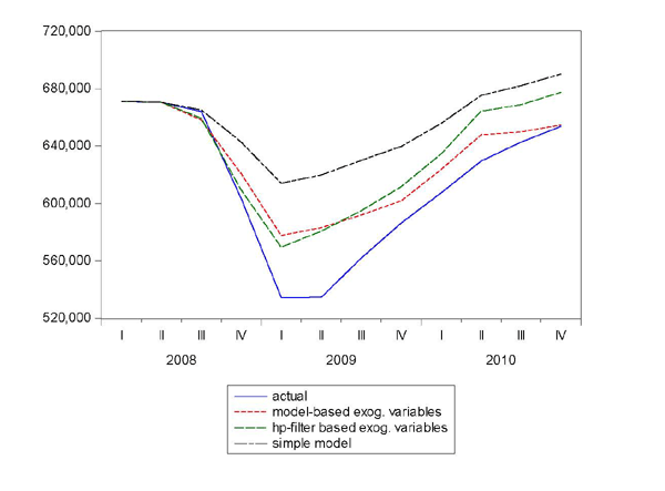
The results are shown in table 4 (root mean squared % errors) and in figures 5 and 6 (forecasts). Forecasts from the models that distinguish trend and cyclical elasticities are better than forecasts from the simple models for about half of the countries, including the United States, Canada, Japan, and Germany. The aggregate forecast error, shown in the last line of the table, is about half the size for the trend/cyclical elasticity models compared with the simple model. As shown in figure 6, the forecasts from these models do not capture all of the cyclical decline that occurred in the past cycle, but they are much closer than the simple model. As shown in table 5, the total decline in exports predicted by the aggregate models is 14-15 percent, compared with 8.5 percent for the simple model and 20.4 percent for the actual.

VII.  Conclusion

Obtaining accurate forecasts of exports during economic cycles is challenging, given that exports tend to be considerably more cyclical than GDP. Models that do not distinguish between trend and cyclical elasticities are likely to understate the swings in exports during cycles, and may correspondingly overstate the elasticity during more tranquil periods. This paper uses a version of the Vahid-Engle estimation of co-integration and co-feature relationships to estimate trend and cyclical elasticities for a total sample of 36 countries. Of this group, both types of elasticities were obtained for 22 countries. As expected, the cyclical elasticities were generally considerably higher than the trend elasticities; the average cyclical elasticity was about 2½ times higher than the average trend elasticity for countries for which both could be estimated.

The methodology was used to derive forecasts that were compared with a simple model that estimates only an average elasticity. The forecasts were better in about half of the cases. For an aggregate of all of the individual forecasts, the models estimated here had a root-mean-squared error that was about half the size of that obtained with the simple model.

This paper represents a first step in this work. Future efforts will be directed at trying to tailor the models more specifically for individual countries and to improving the forecasting techniques for the exogenous variables.

Table 1. Unit Root Tests

	ADF: Exports	ADF: Income	ADF: Ex. Rate	KPSS: Exports	KPSS: Income	KPSS: Ex. Rate
Argentina	-0.874	0.528	-2.252	1.271	1.335	0.370
Belgium-Luxembourg	-0.586	-1.231	-2.895*	1.301	1.329	0.109
Brazil	-0.864	-0.105	-1.997	1.306	1.337	0.933+
Chile	-0.902	0.034	-2.280	1.277	1.335	0.473+
Colombia	-0.658	-0.832	-1.850	1.287	1.332	0.485+
Mexico	-2.609	-1.549	-2.857	1.310	1.332	0.312
Venezuela	-3.029*	-1.017	-1.572	0.433+	1.336	0.260
Austria	-0.772	-1.203	-2.032	1.321	1.323	0.355
Denmark	-1.336	-1.288	-1.917	1.323	1.331	0.704+
Finland	-0.641	-0.816	-1.645	1.286	1.336	0.327
France	-0.776	-1.164	-2.981*	1.321	1.330	0.437
Germany	-0.260	-1.059	-2.424	1.309	1.334	0.331
Greece	-2.631	-1.456	-0.406	1.120	1.324	1.035+
Ireland	-1.527	-1.370	-1.898	1.317	1.329	0.385
Italy	-2.642	-1.013	-2.260	1.273	1.332	0.122
Netherlands	0.384	-1.278	-2.894*	1.299	1.327	0.385
Norway	-1.902	-1.314	-2.823	1.250	1.329	0.137
Portugal	-1.732	-1.308	-1.509	1.279	1.328	1.196+
Sweden	-1.173	-1.198	-2.584	1.314	1.333	0.633+
Singapore	-0.428	-0.487	-2.738	1.328	1.339	0.571+
Spain	-1.295	-1.622	-1.467	1.333	1.326	0.353
Switzerland	-0.228	-1.238	-2.563	1.323	1.330	0.602+
UK	-0.999	-1.199	-2.508	1.300	1.334	0.489+
US	-0.242	-0.739	-1.855	1.292	1.338	0.133
Canada	-2.027	-1.688	-1.470	1.269	1.331	0.267
Japan	-1.018	-0.244	-2.096	1.329	1.342	0.372
China	-2.088	-1.957	-2.639	1.333	1.320	0.880+
Hong Kong	-2.148	1.289	-1.235	1.282	1.342	0.796+
Indonesia	-0.129	-1.024	-2.030	1.281	1.336	0.949+
India	0.392	-0.396	-1.542	1.328	1.338	0.900+
Korea	-0.192	1.124	-2.568	1.345	1.339	0.513+
Malaysia	-0.321	-1.177	-1.586	1.305	1.339	1.091+
Philippines	-0.372	-0.707	-2.561	1.298	1.337	0.303
Taiwan	-1.354	0.721	-0.610	1.323	1.333	0.936+
Thailand	-1.311	-0.658	-1.894	1.325	1.339	1.037+
Vietnam	-0.811	-2.009	-2.459	1.319	1.327	0.209

Critical values for the ADF test: -3.48 (1%); -2.89 (5%); -2.58 (10%)
Critical values for the KPSS test: .739(1%); .463(5%); .347(10%).
*Null hypothesis of a unit root rejected at 5% level.
+Null hypothesis that series is stationary rejected at 5% level.

Table 2. Cointegration Estimation Results

	Two Separate Equations: Income	Two Separate Equations: Exchange Rate	One Equation: Income	One Equation: Exchange Rate
Argentina	1.82*	-6.26*	1.89*	.19
Brazil	1.84*	-2.15*	1.76*	-.05
Chile	2.18*	-4.61*	2.00*	-.44*
Colombia	3.10*	-5.49*	2.79*	-.44*
Mexico	3.19*	8.36*	3.02*	.36
Venezuela	.31	.23*	.18	.21
Austria	2.36*	24.57	2.69*	-2.98*
Denmark	1.74*	3.60	1.75*	-.02
Belgium-Luxembourg	1.54*	16.52*	1.57*	-1.19**
Finland	2.06*	-3.61	2.12*	-.37
France	1.93*	-22.12*	1.87*	-.79**
Germany	1.68*	25.91**	1.84*	-1.28*
Greece	1.00*	2.24*	.76*	.86**
Ireland	3.95*	18.88	4.13*	-1.86*
Italy	1.51*	.62	1.53*	-.51
Netherlands	1.53*	23.68*	1.22*	5.21**
Norway	2.01*	-2.42	1.91*	-1.21
Portugal	2.06*	4.59*	1.58*	1.09
Sweden	1.75*	-1.54	1.76*	-.01
Spain	3.08*	11.45	3.35*	-1.37*
Switzerland	1.60*	11.57*	1.88*	-1.33
UK	1.34*	6.42*	1.29*	.38**
US	1.68*	-5.29	1.80*	-.27
Canada	1.33*	-7.31*	1.55*	-.91*
Japan	1.13*	3.33	1.17*	-.15**
China	4.85*	NA	5.24*	.39
Hong Kong	1.73*	4.35*	1.58*	1.06*
Indonesia	1.47*	-1.47	1.76*	.27*
India	2.86*	NA	2.85*	.21
Korea	2.83*	-14.27*	2.75*	-.35**
Singapore	2.36*	31.88*	2.40*	-.35
Malaysia	2.02*	-2.25*	2.05*	.13
Philippines	1.87*	-15.26	1.89*	.37
Taiwan	2.10*	-5.89*	2.57*	1.20*
Thailand	3.20*	-8.06*	2.62*	-1.41*
Vietnam	5.58*	3.01**	5.60*	-.05

* Significant at 1% level.
** Significant at 5% level.

Table 3. Trend and Cyclical Elasticities

	Model	Income: Trend	Income: Cyclical	Exchange Rate: Trand	Exchange Rate: Cyclical
Argentina	1D	1.82*	9.49**	NA	NA
Brazil	3C	1.84*	2.70	-2.15*	-0.58**
Chile	2A	2.01*	NA	-0.44*	NA
Colombia	2A	2.79*	NA	-0.44*	NA
Mexico	1A	3.19*	NA	NA	NA
Venezuela	-	NA	3.86	NA	-0.48*
Austria	2B	2.69*	2.99*	-2.98*	-2.50*
Denmark	1A	1.74*	NA	NA	NA
Belgium-Luxembourg	2B	1.57*	1.80*	-1.19**	-1.32*
Finland	1C	2.06*	4.30	NA	-1.44**
France	1B	1.93*	3.64*	NA	-2.37*
Germany	2D	1.84*	5.21*	-1.28*	NA
Greece	1D	1.00*	5.88	NA	NA
Ireland	2A	4.13*	NA	-1.86*	NA
Italy	2D	1.53*	3.58	-0.51**	NA
Netherlands	1B	1.53*	3.85*	NA	-2.47*
Norway	1A	2.01*	NA	NA	NA
Portugal	1B	2.06*	2.47**	NA	-2.63
Sweden	1A	1.75*	NA	NA	NA
Spain	2A	3.35*	NA	-1.37*	NA
Switzerland	2B	1.88*	1.94*	-1.33*	-1.49*
UK	1C	1.34*	4.70*	NA	-0.85**
US	1B	1.68*	4.86*	NA	-0.93*
Canada	2D	1.55*	4.41*	-0.91*	NA
Japan	2B	1.17*	8.41*	-0.15**	-0.79**
China	1A	4.85*	NA	NA	-2.03**
Hong Kong	1A	1.73*	NA	NA	NA
Indonesia	1B	1.47*	5.79**	NA	-1.02*
India	1A	2.86*	NA	NA	-1.09*
Korea	2A	2.75*	NA	-0.35**	NA
Singapore	1C	2.36*	5.88*	NA	-2.13**
Malaysia	3C	2.02*	5.98*	-2.25*	-1.05**
Philippines	1C	1.87*	5.51*	NA	-0.76*
Taiwan	1D	2.10*	3.06*	NA	NA
Thailand	2D	2.62*	5.36*	-1.41*	NA
Vietnam	1A	5.58*	NA	NA	NA
Average all countries with trend/ cycle	n/a	2.25	4.59	-1.24	-1.44
Average countries with both trend and cycle	n/a	1.81	4.62	-1.62	-1.29
Average countries with only trend/cycle	n/a	2.98	3.86	-.91	-1.52

* Significant at 1% level.
** Significant at 5% level.

Table 4. Root-Mean-Squared Forecast Errors (%)

	Simple model	Model-based forecasts of exog.	HP-filter based forecasts of exog.
United States	5.10	2.68	3.08
Canada	11.08	7.21	6.73
Japan	23.79	13.40	14.80
United Kingdom	6.53	6.71	10.15
Switzerland	4.06	28.54	12.63
Austria	19.84	22.41	17.30
Belgium/Lux	9.19	3.86	4.79
Finland	20.87	52.51	38.44
France	3.86	16.89	4.82
Germany	8.51	5.92	5.13
Greece	27.16	10.59	12.47
Italy	12.35	41.02	29.55
Netherlands	2.98	37.26	22.38
Portugal	10.30	6.31	3.92
Argentina	19.74	89.87	50.19
Brazil	11.34	19.24	19.72
Taiwan	15.81	13.08	15.95
Singapore	3.27	5.44	5.55
Malaysia	16.59	21.90	41.11
Philippines	10.79	11.66	14.39
Indonesia	12.40	24.72	15.73
Thailand	21.93	4.11	9.51
Aggregate exports	9.12	4.42	4.87

Table 5. Percent Change in Aggregate Exports, 2008: Q1-2009:Q1

Actual	Simple model	Model-based forecasts of exog. variables	HP-filter based forecasts of exog. variables
-20.4	-8.5	-13.9	-15.1

Appendix:  Decomposition of Exports and Output into Trend and Cyclical Components

For models 1B, 1C, and 1D (exports and output have unit roots, exchange rates do not):

X = X_p + X_c

I = I_p + I_c

E = E_m + E_c

X_p = $\alpha$_p + $\beta$_p * I_p

For model 1B:

X_c = $\alpha$_c + $\beta$_c * I_c

X_c = $\delta$_c + $\gamma$_c * E_c

I_p = (X - ($\alpha$_p + $\alpha$_c) - $\beta$_c * I)/($\beta$_p - $\beta$_c)

For model 1C:

X_c = $\alpha$_c + $\beta$_c * I_c + $\gamma$_c * E_c

I_p = (X - ($\alpha$_p + $\alpha$_c) - $\beta$_c * I - $\gamma$_c *(E- E_m)/($\beta$_p - $\beta$_c)

For model 1D:

X_c = $\alpha$_c + $\beta$_c * I_c

I_p = (X - ($\alpha$_p + $\alpha$_c) - $\beta$_c * I)/($\beta$_p - $\beta$_c)

For models 2B and 2D (exports and output, and exchange rates all have unit roots and there is one co-integrating relationship):

X_p = $\alpha$_p + $\beta$_p * I_p + $\gamma$_p * E_p

For model 2B:

X_c = $\alpha$_c + $\beta$_c * I_c

X_c = $\delta$_c + $\gamma$_c * E_c

Y_p = (X - ($\alpha$_p+$\alpha$_c+$\gamma$_p/$\gamma$_c*( $\delta$_c - $\alpha$_c)-$\beta$_c*(1- $\gamma$_p/$\gamma$_c)*I)-$\gamma$_p*E) /($\beta$_p + $\beta$_c*(1-$\gamma$_p/$\gamma$_c)) For model 2D:

X_c = $\alpha$_c + $\beta$_c * I_c

I_p = (X - ($\alpha$_p + $\alpha$_c) - $\beta$_c * I) - $\gamma$_p * E) /($\beta$_p - $\beta$_c)For model 3C (two co-integrating relationships and one co-feature relationship with both variables):

X_p = $\alpha$_p + $\beta$_p * I_p

X_p = $\delta$_p + $\gamma$_p * E_p

X_c = $\alpha$_c + $\beta$_c * I_c + $\gamma$_c * E_c

I_p = (X - ($\alpha$_p+ $\alpha$_c + $\gamma$_p/$\gamma$_c*( $\delta$_p - $\alpha$_p) - $\beta$_c * I - $\gamma$_c * E) /($\beta$_p *(1-$\gamma$_c/$\gamma$_p) - $\beta$_c)

Figure 1. World Exports and GDP Year-Over-Year % Change

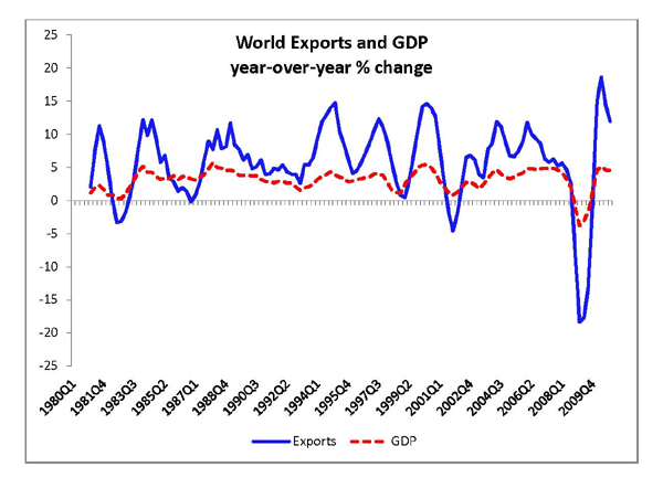
Figure 2a. World Exports and GDP Year-Over-Year % Change

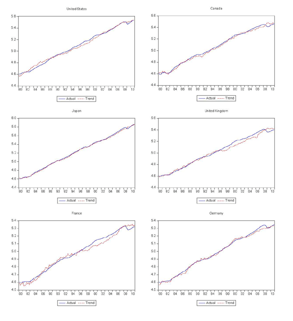
Figure 2b. World Exports and GDP Year-Over-Year % Change (cont'd)

Figure 2c. World Exports and GDP Year-Over-Year % Change (cont'd)

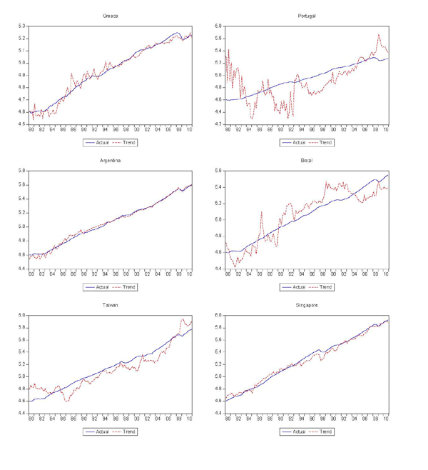
Figure 2d. World Exports and GDP Year-Over-Year % Change (cont'd)

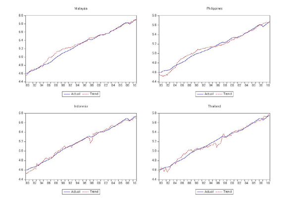
Figure 3a. Actual and Trend Exports

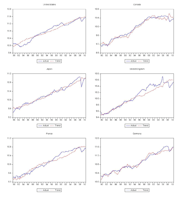
Figure 3b. Actual and Trend Exports (cont'd)

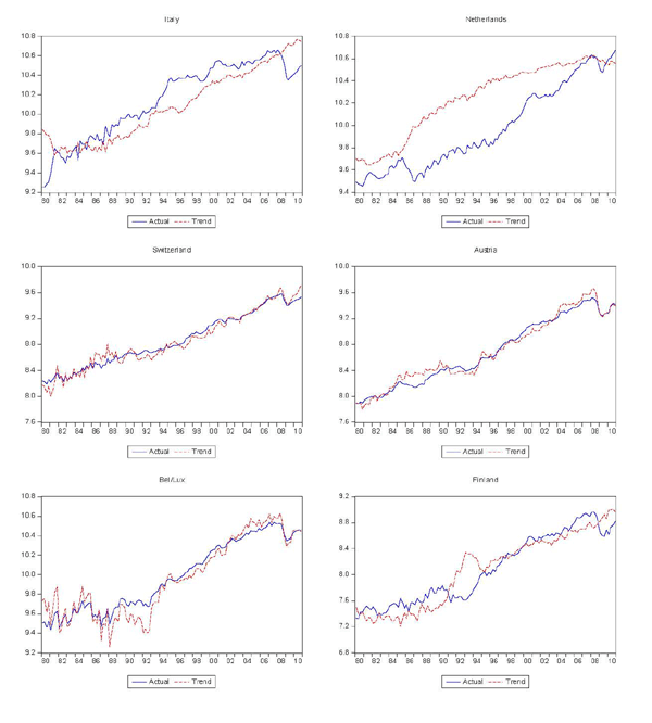
Figure 3c. Actual and Trend Exports (cont'd)

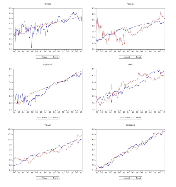
Figure 3d. Actual and Trend Exports (cont'd)

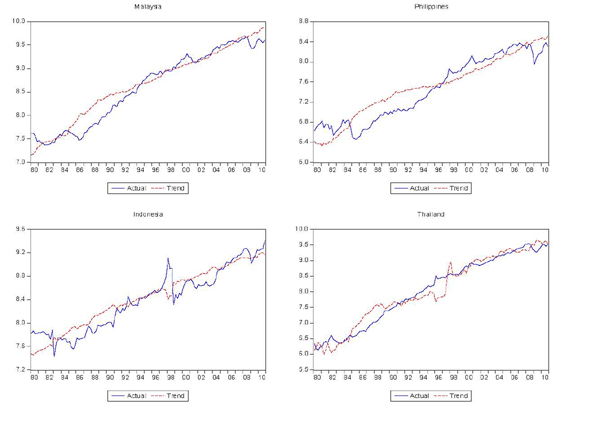
Figure 4a. Cyclical Components of Trading Partner GDP and Exports

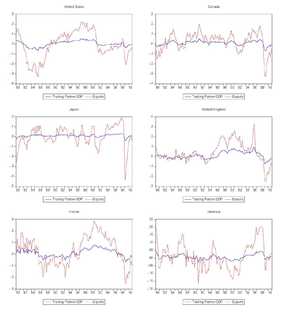
Figure 4b. Cyclical Components of Trading Partner GDP and Exports (cont'd)

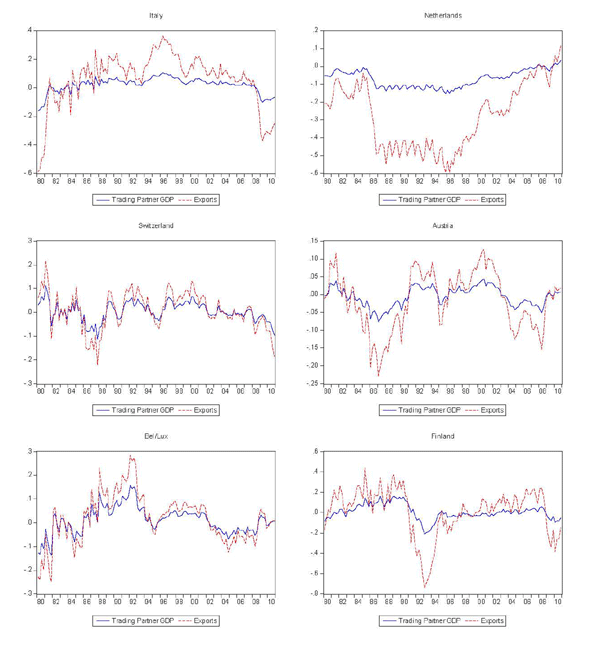
Figure 4c. Cyclical Components of Trading Partner GDP and Exports (cont'd)

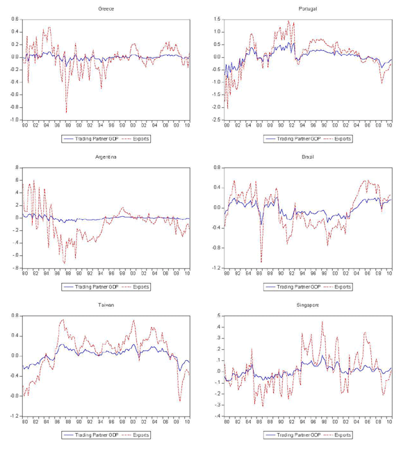
Figure 4d. Cyclical Components of Trading Partner GDP and Exports (cont'd)

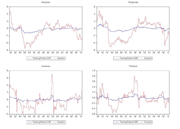
Figure 5a. Comparison of Export Forecasts

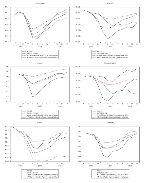
Figure 5b. Comparison of Export Forecasts (cont'd)

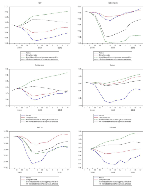
Figure 5c. Comparison of Export Forecasts (cont'd)

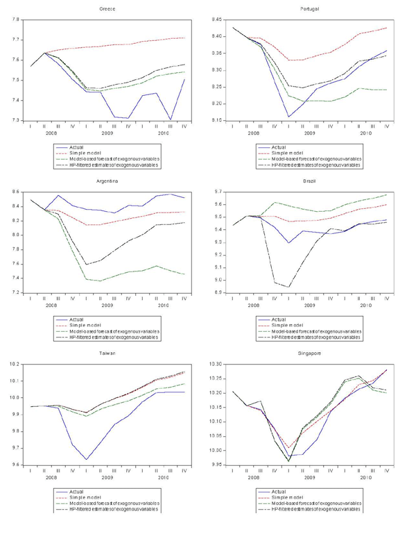
Figure 5d. Comparison of Export Forecasts (cont'd)

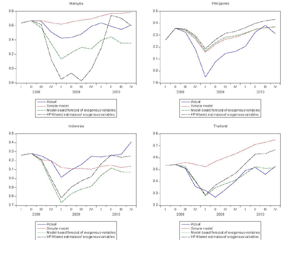
Figure 6. Comparison of Export Forecasts Summed

References

Clavijo, F., and R. Faini, "Differentiating Cyclical and Long-Term Income Elasticities of Import Demand," Policy, Planning, and Research Working Paper 197, the World Bank, May 1989.

Carvalho, V., A. Harvey, and T. Trimbur, "A Note on Common Cycles, Common Trends, and Convergence," Journal of Business and Economic Statistics, vol. 25, (2007), pp.12-20.

Caporale, G.M., and M.K.F. Chui, "Estimating Income and Price Elasticities of Trade in a Cointegration Framework," Review of International Economics, 7(2), (1999), pp. 254-264.

Engel, C., and J. Wang, "International Trade in Durable Goods: Understanding Volatility, Cyclicality, and Elasticities," Journal of International Economics, 83 (2011), pp. 37-52.

Fadiga, M., and S. K. Misra, "Common trends, Common Cycles, and Price Relationships in the International Fiber Market," Journal of Agricultural and Resource Economics, 32(1) (2007), pp. 154-168.

Gu, B., and H.S. Lee, "Common Trends, Common Cycles and Forecasting," The Journal of the Korean Economy, vol. 8, #2 (Fall 2007), pp. 305-327.

Kapetanios, G., "A Note on Joint Estimation of Common Cycles and Common Trends in Nonstationary Multivariate Systems," Working Paper # 483, Queen Mary, University of London (2003).

Kugler, P. "The Common Trend and Common Cycle of Exports and the Real Exchange Rate: Empirical Results from Swiss Data," Weltwirtschaftliches Archiv, vol. 136(1), (2000), pp. 171-180.

Senhadji, A., and C. Montenegro, "Time Series Analysis of Export Demand Equations: A Cross-Country Analysis," Working Paper 98/149, IMF (1998).

Vahid, F., and R. Engle, "Common Trends and Common Cycles," Journal of Applied Econometrics," vol. 8, (1993), pp. 341-360.

Footnotes

**  The author is a Senior Advisor in the Division of International Finance. Mailing address: Division of International Finance, Board of Governors of the Federal Reserve System, Mail Stop 20, Washington D.C. 20551, U.S.A. Email: [email protected]. Telephone: (202)-452-2374; fax (202)-263-4850. Return to text

1.   United States, Austria, Belgium/Luxembourg, Denmark, Finland, France, Germany, Greece, Ireland, Italy, the Netherlands, Norway, Portugal, Sweden, Switzerland, Spain, United Kingdom, Canada, Japan, China, Hong Kong, Taiwan, South Korea, Singapore, Malaysia, the Philippines, Thailand, Indonesia, India, Vietnam, Argentina, Brazil, Chile, Colombia, Mexico, and Venezuela.  Return to text

This version is optimized for use by screen readers. Descriptions for all mathematical expressions are provided in LaTex format. A printable pdf version is available. Return to text

Home | Economic research and data | Publications and education resources
Accessibility | Contact us
Last update: September 30, 2011