International Relative Price Levels: A Look Under the Hood

Jaime Marquez, Charles Thomas, and Corinne Land¹

NOTE: International Finance Discussion Papers are preliminary materials circulated to stimulate discussion and critical comment. References in publications to International Finance Discussion Papers (other than an acknowledgment that the writer has had access to unpublished material) should be cleared with the author or authors. Recent IFDPs are available on the Web at http://www.federalreserve.gov/pubs/ifdp/. This paper can be downloaded without charge from the Social Science Research Network electronic library at http://www.ssrn.com/.

Abstract:

This paper examines the structure of international relative price levels using purchasing power parities (PPP) at the product-level from the 2005 World Bank's International Comparison Program (ICP). Our examination is motivated by questions arising from two applications using economy-wide PPPs: the measurement of real effective exchange rates (REERs) and the correlation between prices and development. Specifically, how would our view on competitiveness be affected if one were to use PPP measures that exclude non-tradable categories? Is it the case that an increase in per-capita income raises the prices of non-tradable categories? These questions are not new. What is new here is the use of relative price levels (as opposed to indexes) at the product level for 144 countries that differ greatly in their level of development.

Keywords: International comparison program, purchasing power parity, competitiveness, penn effect, real effective exchange rates, tradability

JEL classification: F41, F43

1 Introduction

Economy-wide PPPs provide information on international relative price levels and hence capture a dimension of competitiveness not incorporated in indexes that measure price changes alone.³ But a relevant question, so far neglected, is how would our view on competitiveness be affected if one were to use PPP measures that exclude non-tradable categories? In addition, since it is acknowledged that prices for some categories are particularly difficult to compare across countries, to what extent are PPP-based GDP price comparisons being influenced by the readings on these "comparison-resistant" categories? Our calculations indicate that excluding comparsion-resistant categories halves the measured difference between U.S. prices and the prices of its major trading partners; excluding non-tradable categories eliminates the difference entirely. The obvious question raised by this finding is which measure is better for making inferences about international competitiveness: the measure including all the expenditure categories or the narrower measures including only tradable or comparable products? Though we do not have a definitive answer to this question, we follow Keynes (1925) and Corden (1994) and show that prices for non-tradable and comparison-resistant categories play an integral role in measuring international competitiveness.

The correlation between aggregate prices and development, known as the Penn Effect, has been examined extensively. The conventional explanation for this correlation is that as development expands, demand across all expenditure categories increases, which raises the prices of non-tradables but not the prices of tradables because these are determined in world markets. This explanation raises an interesting question: is it the case that an increase in per-capita income raises the relative prices of non-tradable categories? This question has not been addressed before and an answer to it is of interest because finding that these correlations are absent would undermine the conventional explanation for the Penn Effect. To be sure, interest in disaggregation is not new.⁴ What is new here is the use the relative price levels (as opposed to indexes) at the product level for 144 countries that differ greatly in their level of development.

The next section describes the data; section 3 lays out the basic constructs of our PPP-based REER and demonstrates its sensitivity to the exclusion of non-tradable and non-comparable categories. Section 4 reports the results from regressions relating the within-product relative prices to relative incomes. Section 5 offers a few concluding thoughts.

2 Data Description

2.1 ICP Data

The ICP provided the 2005 benchmark purchasing power parities for 146 countries and 126 basic headings;⁵ a " basic heading" is the lowest level of disaggregation for which PPPs are computed.⁶ The ICP also provided country data on population, market exchange rates, the 2005 values for GDP, PPPs for GDP, and expenditures on each basic headings; these expenditures add up to GDP.

Reliance on the 2005 ICP benchmarks has several advantages. First, they are the first to include actual price observations for China, and the first since 1985 to include actual price observations for India.⁷ Second, the ICP differentiates between government expenditures and private expenditures, facilitating international price comparisons. Finally, data collection uses the concept of "Structured Product Descriptions," which is a list of standardized attributes that identifies a product as narrowly as possible, enhancing product comparability.⁸These detailed descriptions allow the ICP to identify several basic headings as comparison-resistant: government production of health services, collective services, social protection, education, and various medical services.

The ICP does not provide, however, a taxonomy of basic headings as being tradable or not; indeed, developing a widely accepted taxonomy of tradability has remained elusive.⁹ Thus, given the difficulties of concisely defining tradability, we use a subjective but, we believe, reasonable classification of basic headings as tradable. However, one of the advantages of using the disaggregated price data is that one can examine the implications of alternative definitions by re-grouping the basic headings accordingly. So, our definition is ad-hoc but it is not rigid.

2.2 Cross-Country Distributions of Relative Prices

We measure the 2005 bilateral price level of the United States with respect to country in basic heading as

$\displaystyle q_{j,us}^{i}=\frac{E_{\frac{j}{\$}}}{PPP_{\frac{j}{us}}^{i}}$ , $\displaystyle i=1,...126;$ $\displaystyle j=1,...,144,$

(1)

where $E_{\frac{j}{\$}}$ is the 2005 market exchange rate for country with respect to the U.S. dollar and $PPP_{\frac{j}{us}}^{i}$ is the PPP exchange rate of the basic heading in the country, defined as $\frac {P_{j}^{i}}{P_{us}^{i}}$ where $P_{j}^{i}$ is the price level (local currency per unit) of the basic heading in the country. A value of 2 for $q_{j,us}^{i}$ means that the price of the basic heading in the United States is twice that of the same basic heading in country , when both are expressed in a common currency.

Given equation (1), we assemble the cross-country distributions of relative prices for each basic heading to examine two questions: Are the prices of a given basic heading equalized across countries?¹⁰ Is the dispersion of relative prices across countries related to whether the product is tradable?

Figure 1 shows the cross-country distributions of relative prices ( $q_{j,us}^{i}$ ) for each basic heading; the figure shows the basic headings that the ICP identifies as comparison resistant and the basic headings that we identify as tradable and non-tradable. For each distribution, we show the median and four percentiles; these distributions are arranged in descending order of their medians. The data show that most of the medians are well above one, especially for comparison-resistant products. Further, the medians of the distributions for tradable products are generally lower than those for non-tradable products. Finally, the dispersion of relative prices for non-tradables is considerably larger than that for tradables. These properties resonate with our priors that international trade tends to equate prices across countries and that this tendency is greatest for the most readily tradable products.

3 U.S. Relative Price Levels in 2005

We now assess the importance of the product mix for measuring U.S. international relative price levels. To this end, we begin by assembling the cross-country distributions of relative prices for the largest trading partners of the United States.¹¹ Figure 2 shows that the median for most of these distributions is quite close to one and well below the median for the distributions using 144 countries. To emphasize the importance of the country mix, figure 3 compares the distributions of relative prices without differentiating across basic headings. The figure shows that the cross-country distribution of relative prices for U.S. trading partners is considerably narrower and more symmetrical than the one for the 144 countries.

To provide some perspective on what we are after, figure 4 depicts U.S. relative price levels based on the ICP's published GDP parities for the 34 countries included in figure 2. By this measure, U.S. GDP prices were twice as high as the GDP prices in India and 30 percent below those in Switzerland. The question of interest is to what extent are these measures of relative prices influenced by the prices of basic headings that are either non-tradable or comparison-resistant?

Addressing this question involves two steps. The first one is to measure the aggregate relative price level between the United States and the trading partner using alternative basic headings. To this end, we use a weighted geometric average:

$\displaystyle q_{j,L}= {\textstyle\prod\limits_{i\in L}} \left( q_{j,us}^{i}\right) ^{w_{ij,L}},j=1,...,34,$

(2)

where is a list of basic headings, $q_{j,us}^{i}$ is defined in equation (1), $w_{ij,L}$ is the share of the country's expenditure on the basic heading, and $\sum_{i\in L}w_{ij,L}=1$ . A value of 2 for $q_{jL}$ means that U.S. prices are twice as high as those in the country in list . We consider three lists:

$\qquad L_{1}$ : All headings

$\qquad L_{2}$ : Authors' defined tradable headings

$\qquad L_{3}$ : All headings excluding ICP's " comparison resistant" headings

The second step is to map the $q_{j,L}$ into alternative measures of the U.S. real effective exchange rate. To this end, we use a weighted geometric mean:

$\displaystyle Q_{L}= {\textstyle\prod\limits_{j=1}^{34}} \left( q_{j,L}\right) ^{\delta_{j}},L=L_{1},L_{2},L_{3},$

(3)

where $Q_{L}$ is the level of the U.S. real effective exchange rate for list , $q_{j,L}$ is defined in equation (2), and $\delta_{j}$ is the U.S. bilateral trade weight associated with the country.¹² A value of 2 for $Q_{L}$ means that the aggregate of U.S. prices in list is twice as high as the average of aggregate prices of U.S. trading partners in the same list.

Figure 5 reports our calculations. As a check on our procedures, we compare the "all-headings" measure $q_{j,L_{1}}$ to the published ICP's GDP relative prices, denoted as $q_{j,GDP}$ and shown earlier in figure 4. Excluding Thailand and Malaysia, the two measures are very close and two factors help explain this gap. First, $q_{j,L_{1}}$ is measuring prices of domestic expenditures whereas $q_{j,GDP}$ is measuring prices of expenditures on domestic products-that is, excluding imports and including exports. Second, equation (2) might differ from the one used by the ICP.

Taking $q_{j,L_{1}}$ as our benchmark of economy-wide relative prices, we find that the relative-price measure excluding non-tradable headings ( $q_{j,L_{2}}$ ) shifts down the structure of U.S. relative price levels with the shift being particularly pronounced vis-à-vis emerging economies. For example U.S. aggregate prices are measured to be 105 percent above those in India; whereas, if we exclude non-tradable headings, the gap shrinks to 60 percent. In contrast, vis-à-vis Switzerland, the measured differential shrinks by only one percent with the exclusion of non-tradables. The relative-price measure excluding comparison-resistant headings ( $q_{j,L_{3}}$ ) also shifts down the structure of relative prices, but to a lesser extent than when prices in non-tradable headings are excluded.

The rightmost column of figure 5 shows the sensitivity of $Q_{L}$ to changes in the mix of basic headings. Specifically, if one includes the prices of all headings ( $Q_{L_{1}}$ ), then U.S. prices appear to be 25 percent above the average of its trading partners. If we exclude prices of headings that are difficult to compare across countries, then the measured wedge shrinks to about 10 percent ( $Q_{L_{2}}$ ). Finally, if we limit ourselves to prices for tradable basic headings ( $Q_{L_{3}}$ ), then there appears to be little difference between U.S. prices and the average of prices of its major trading partners.

This finding suggests that excluding either comparison-resistant or non-tradable basic headings from the product mix lowers the measure of U.S. relative prices. We do not take this finding as evidence for designating either $Q_{L_{2}}$ or $Q_{L_{3}}$ as the better measure for making inferences about international competitiveness. Rather, we consider the comparison-resistant and non-tradable basic headings essential to analyzing international price positions.

Our view is not new. Indeed, Keynes noted in 1925 (p. 301): " it is the price of sheltered [non-tradable] goods that determines the competitiveness of a country because it is those prices that determine the cost of producing tradable goods. The price of unsheltered goods will be equalized by trade."¹³ Further, Keynes' view is formalized by Corden (1994, p. 267) who argues that a country's international competitiveness is determined by the profitability in industries producing tradables. Specifically, Corden measures international competitiveness in the industry as the ratio of the country's price markup to that of the United States:

$\displaystyle \rho_{i}=\left( \frac{P_{j,i}}{MC_{j,i}}\right) /\left( \frac{P_{us,i} }{MC_{us,i}}\right) ,$

(4)

where $P_{j,i}$ is the dollar price of the tradable industry in the country, and $MC_{j,i}$ is the associated marginal cost, also in dollars. Thus, if $\rho_{i}>1$ , then the country is said to be more competitive than the United States because it has a higher price markup. Further, if one assumes that international trade equalizes prices of tradable products, then

$\displaystyle \rho_{i}=\left( \frac{P_{i}}{MC_{j,i}}\right) /\left( \frac{P_{i} }{MC_{us,i}}\right) =\frac{MC_{us,i}}{MC_{j,i}}.$

(5)

Again, if $\rho_{i}>1$ , then the country is more competitive than the United States because it has lower marginal costs. Marginal costs are directly related to factor prices, such as wages that are, in turn, directly related to the importance of non-tradables (e.g. housing, medical services) in domestic expenditures. Given that comparison-resistant and non-tradable basic headings account for more than half of U.S. total domestic expenditures (figure 6), abstracting from them yields an incomplete characterization of international competitiveness.

4 Development and Relative Price Levels

In this section we study the correlation between the level of economic development and the level of relative prices across countries, known as the Penn Effect. Intuitively, higher levels of income raise the demands for tradable and non-tradable goods and services. The higher demand for tradables is met through international trade with no change in tradable's prices. But the higher demand for non-tradables is met by the fixed, local supply, raising the price of non-tradables and, thus, the overall price level. So the natural question to ask is whether the data support the view that an increase in income raises the relative prices of non-tradable categories.

To this end, we begin by replicating the Penn Effect and postulate that

$\displaystyle \ln q_{GDP}=\alpha+\beta\cdot\ln y+u,$ $\displaystyle u\symbol{126}N(0,\sigma^{2}),$

(6)

where

$\qquad q_{GDP}=(q_{1,GDP}\cdots q_{144,GDP})^{\prime}$

$\qquad q_{j,GDP}$ is the U.S. price relative to the price of the

country using ICP's published GDP parities

$\qquad y=(\frac{y_{1}}{y_{us}}\cdots\frac{y_{144}}{y_{us}})^{\prime}$

$\qquad\frac{y_{j}}{y_{us}}=(\frac{GDP_{j}}{POP_{j}}\cdot\frac {1}{PPP_{\frac{j}{\$}}})/\frac{GDP_{us}}{POP_{us}}$

$GDP_{j}$ is the GDP of the

country

$POP_{j}$ is the population of the

country

For the conventional explanation of the Penn Effect to be consistent with the aggregate data, one needs to find that $\beta<0$ : An increase in the per-capita income of the country relative to U.S. per-capita income raises the price in the country relative to the corresponding U.S. price and, hence, lowers $q_{j,GDP}$ . The regression yields

$\begin{displaymath} \begin{array}[c]{lcl} \text{ln$q$}_{GDP} & = & \begin{array}[t]{r} 0.1715\ ^{(0.0502)} \end{array}\ -\! \begin{array}[t]{r} 0.2354\ ^{(0.0219)} \end{array}\text{ln$y$} \end{array}, \end{displaymath}$

where the standard errors of the coefficients are corrected for potential heteroskedasticity of the residuals.¹⁴ The result confirms that $\beta<0$ when using the ICP's published parities for GDP.

To examine whether this correlation holds at the level of basic headings, we use

$\displaystyle \ln q_{i}=\alpha_{i}+\beta_{i}\cdot\ln y+u_{i},$ $\displaystyle i=1,...,126,$ $\displaystyle u_{i}\symbol{126}N(0,\sigma_{i}^{2}),$

(7)

where $q_{i}=(q_{1,us}^{i}\cdots q_{144,us}^{i})^{\prime}$ and $q_{j,us}^{i}$ is defined in equation (1). For the conventional explanation of the Penn Effect to be consistent with the data at the disaggregate level, one needs to find that $\beta_{i}<0:$ An increase in the per-capita income of the country relative to U.S. per-capita income tends to raise the price of the good in the country relative to the corresponding U.S. price, which then lowers $q_{j,us}^{i}$ . Thus finding that $\beta_{i}=0$ for non-tradables would undermine the usefulness of the conventional explanation for the Penn Effect.

Figure 7 shows the estimates of $\beta_{i}$ and their 95 percent confidence bands.¹⁵ For the vast majority of basic headings, the estimated $\beta_{i}$ is negative and significantly different from zero. That is, for most of the basic headings, higher prices in the country are associated with higher incomes in the country. We also note that the estimates of $\beta_{i}$ tend to be larger (in absolute value) for the headings that we denoted non-tradables than for the headings we denoted tradables. This finding strengthens the empirical support of the conventional explanation of the Penn Effect.

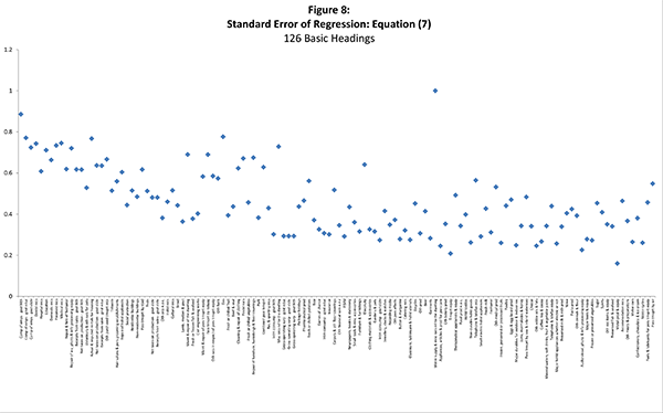
This pattern for the $\beta_{i}$ s is not a necessary consequence of the pattern seen in figure 1, as the estimated intercept could absorb the variation in the medians. Indeed, the estimated standard errors of the regressions bear no relationship to the ordering of the basic headings (figure 8). Finally, note that for three of these products (motorcars, motorcycles, and passenger transport by air), the estimated $\beta$ is significantly positive, meaning that higher prices are associated with lower incomes, a deviation from the Penn Effect. This seemingly contradictory finding might be the result of some countries treating these products as luxuries and thus levying taxes on them.

5 Conclusions

The view under the hood yields two insights that might be useful for practical analyses and further research.

First, we get a good sense of the extent to which the real effective exchange rate for the United States is affected by the inclusion of non-tradable prices. For 2005, with the full product list, the U.S. REER shows U.S. prices to be more than 20 percent above those of its trading partners, while for tradable products alone, there is little difference between U.S. prices and those of its trading partners. We do not view this sensitivity as an argument for excluding non-tradables when judging competitiveness because the prices of non-tradables are central to determining a country's profitability in tradable products.

Second, the Penn Effect is not an artifact of aggregation. Indeed we find that this effect holds for the majority of basic headings. Interest in this disaggregation is not new but previous work uses aggregate price indexes for selected sectors of industrial countries. In contrast, we offer evidence based on relative price levels (as opposed to indexes) of 126 basic headings for 144 countries that differ greatly in their level of development. This generality makes the Penn Effect an interesting subject for future research because it does not rely on aggregation formulas.

Figure 1: Distribution of Relative Prices (Pus/Pi) -- Log Scale

Figure 1 shows the cross-country distributions of relative prices for each basic heading; the figure shows the basic headings that the ICP identifies as comparison resistant and the basic headings that we identify as tradable and non-tradable. For each distribution, we show the median and four percentiles; these distributions are arranged in descending order of their medians. The data show that most of the medians are well above one, especially for comparison-resistant products. Further, the medians of the distributions for tradable products are generally lower than those for non-tradable products. Finally, the dispersion of relative prices for non-tradables is considerably larger than that for tradables. These properties resonate with our priors that international trade tends to equate prices across countries and that this tendency is greatest for the most readily tradable products.

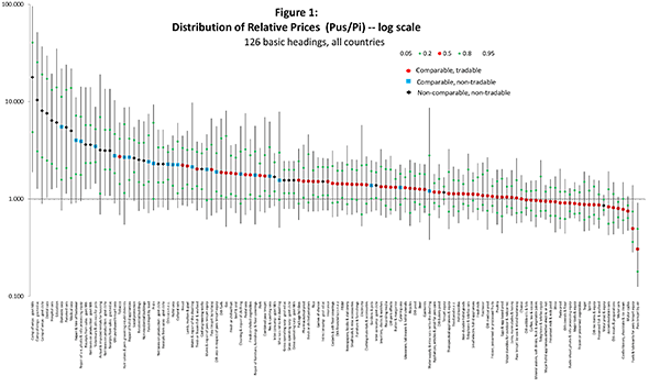
Figure 2: Distribution of Relative Prices -- Log Scale

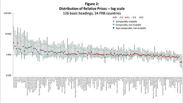
Figure 2: We now assess the importance of the product mix for measuring U.S. international relative price levels. To this end, we begin by assembling the cross-country distributions of relative prices for the largest trading partners of the United States.This figure shows that the median for most of these distributions is quite close to one and well below the median for the distributions using 144 countries.

Figure 3: Histogram of Relative Prices - Ln(Pus/Pi)

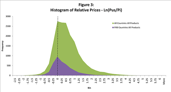
Figure 3: Compares the distributions of relative prices without differentiating across basic headings. The figure shows that the cross-country distribution of relative prices for U.S. trading partners is considerably narrower and more symmetrical than the one for the 144 countries.

Figure 4: Published Domestic Expenditures Ln Relative Prices (Pus/Pi)

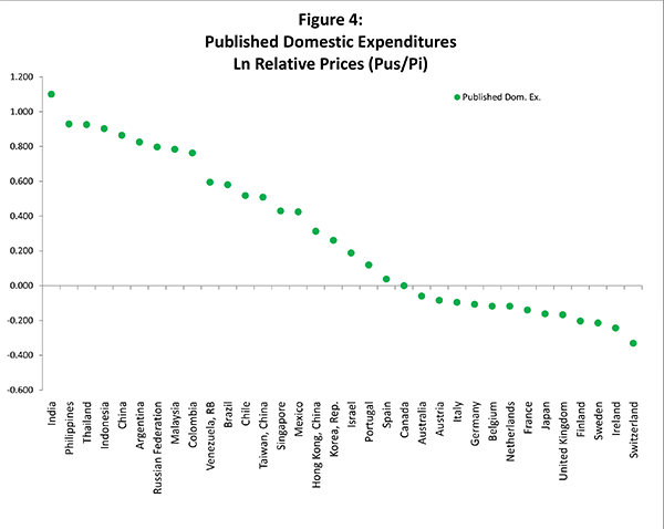
Figure 4: Depicts U.S. relative price levels based on the ICP's published GDP parities for the 34 countries included in figure 2. By this measure, U.S. GDP prices were twice as high as the GDP prices in India and 30 percent below those in Switzerland.

Figure 5: Selected Domestic Expenditure Groupings Ln Relative Prices (Pus/Pi)

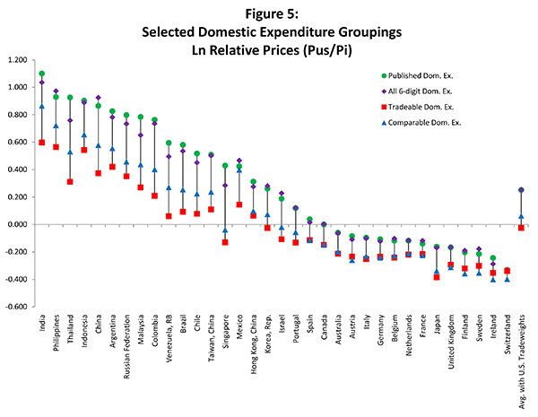
Figure 5: Reports our calculations. As a check on our procedures, we compare the all-headings measure to the published ICP's GDP relative prices, denoted as and shown earlier in figure 4. Excluding Thailand and Malaysia, the two measures are very close and two factors help explain this gap. First, is measuring prices of domestic expenditures whereas is measuring prices of expenditures on domestic products-that is, excluding imports and including exports. Second, equation (2) might differ from the one used by the ICP.

Figure 6: Selected Expenditure Shares

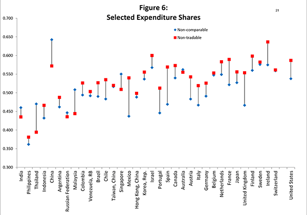
Figure 6: Marginal costs are directly related to factor prices, such as wages that are, in turn, directly related to the importance of non-tradables (e.g. housing, medical services) in domestic expenditures. Given that comparison-resistant and non-tradable basic headings account for more than half of U.S. total domestic expenditures, abstracting from them yields an incomplete characterization of international competitiveness.

Figure 7: Corrrelation Between Relative Prices and Development: 95% Confidence Band

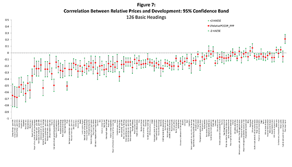
Figure 7: Shows the estimates of Beta sub i and their 95 percent confidence bands.15 For the vast majority of basic headings, the estimated Beta sub i is negative and significantly different from zero. That is, for most of the basic headings, higher prices in the jth country are associated with higher incomes in the jth country. We also note that the estimates of Beta sub i tend to be larger (in absolute value) for the headings that we denoted non-tradables than for the headings we denoted tradables. This finding strengthens the empirical support of the conventional explanation of the Penn Effect.

Figure 8: Standard Error of Regression: Equation (7)

Figure 8: This pattern for the Beta sub i s is not a necessary consequence of the pattern seen in figure 1, as the estimated intercept could absorb the variation in the medians. Indeed, the estimated standard errors of the regressions bear no relationship to the ordering of the basic headings (figure 8). Finally, note that for three of these products (motorcars, motorcycles, and passenger transport by air), the estimated Beta is significantly positive, meaning that higher prices are associated with lower incomes, a deviation from the Penn Effect. This seemingly contradictory finding might be the result of some countries treating these products as luxuries and thus levying taxes on them.

References

Asea P. and E. Mendoza, 1994, " The Balassa-Samuelson Model: A General-Equilibrium Appraisal," Review of International Economics, 2, 244-267.

Bergin, P., R. Glick, and A. Taylor, 2006, "Productivity, Tradability, and the Long-run Price Puzzle," Journal of Monetary Economics, 53, 2041-2066.

Canzoneri, M., R. Cumby, B. Diba, 1996, "Relative Labor Productivity and the Real Exchange Rate in the Long Run: Evidence for a Panel of OECD Countries," NBER Working Paper, No. 5676.

Chen, S. and M. Ravallion, 2008, "China is Poorer than we Thought, But No Less Successful in the Fight Against Poverty," World Bank Policy Research Working Paper, No. 4621.

Chinn, M., 2005, "A Primer on Real Effective Exchange Rates: Determinants, Overvaluation, Trade Flows and Competitive Devaluation," NBER Working Paper, No. 11521.

Corden, M., 1994, Economic Policy, Exchange Rates, and the International System, Chicago: University of Chicago Press.

De Gregorio, J., A. Giovannini, and H. Wolf, 1994, "International Evidence on Tradables and Nontradables Inflation," European Economic Review, 38, 1225-1244.

Doornik, J. and D. Hendry, 2007, Empirical Econometric Modeling, London: Timberlake.

Froot, K. and K. Rogoff, 1995, "Perspectives on PPP and Long-run Real Exchange Rates," in G. Grossman and K. Rogoff (eds.), Handbook of International Economics, vol 3., Amsterdam: North-Holland.

Heston, A., R. Summers and B. Aten, 2006, Penn World Table Version 6.2, Center for International Comparisons of Production, Income and Prices at the University of Pennsylvania.

Hooper, P. and J. Richardson (eds.), 1991, International Economic Transactions: Issues in Measurement and Empirical Research, Chicago: University of Chicago Press.

Isard, P., 1977, "How Far Can We Push the Law of One Price?" American Economic Review, 67, 942-948.

Keynes, J., 1925, " The Committee on the Currency," The Economic Journal, 138, 299-304.

Klau, M. and S. Fung, 2006, "The New BIS Effective Exchange Rate Indices," BIS Quarterly Review, March, 51-65.

Kravis, I., A. Heston, and R. Summers, 1978, International Comparisons of Real Product and Purchasing Power, Baltimore: Johns Hopkins University Press.

Kravis, I. and R. Lipsey, 1990, "The International Comparison Program: Current Status and Problems," NBER Working Paper, No. 3304.

Leahy, M., 1998, "New Summary Measures of the Foreign Exchange Value of the Dollar," Federal Reserve Bulletin, October, 811-18.

Lipsey, R., L. Molinari, and I. Kravis, 1990, "Measures of Prices and Price Competitiveness in International Trade in Manufactured Goods," NBER Working Paper, No. 3442.

Lothian, J. and M. Taylor, 2008, "Real Exchange Rates Over the Past Two Centuries: How Important is the Harrod-Balassa-Samuelson Effect?" Economic Journal, 118, 1742-1763.

Ravallion, M., 2010, "Price Levels and Economic Growth: Making Sense of the PPP Changes Between ICP Rounds," World Bank Policy Research Working Paper, No. 5229.

Summers, R. and A. Heston, 1991, "The Penn World Table (Mark 5): An Expanded Set of International Comparisons, 1950-1988," Quarterly Journal of Economics, 106, 327-368.

Taylor, M., 2003, "Purchasing Power Parity," Review of International Economics, 11, 436-452.

Thomas, C., J. Marquez, and S. Fahle, 2008, "Measuring U.S. International Relative Prices," Federal Reserve Board International Finance Discussion Paper, No. 917.

Thomas, C., J. Marquez, J. Coonan, and S. Fahle, 2011, " International Relative Price Levels: Stylized Facts," in F. Vogel and D.S. Prada Rao (editors), Measuring the Size of The World Economy: A Framework, Methodology and Results from the International Comparison Program, Washington DC: World Bank, forthcoming.

Turner, P. and J. Van't dack, 1993, "Measuring International Price and Cost Competitiveness," BIS Economic Papers, No. 39.

World Bank, 2008, Global Purchasing Power Parities and Real Expenditures: 2005 International Comparison Program, Washington DC: World Bank.

Footnotes

* The views in this paper are solely the responsibility of the authors and should not be interpreted as reflecting the views of the Board of Governors of the Federal Reserve System or of any other person associated with the Federal Reserve System. We are grateful to Nada Hamadeh for providing the ICP data and to both Fred Vogel and D.S. Prasada Rao for numerous comments. We are also grateful to Rudolfs Bems, Neil Ericsson, and to participants in previous presentations of this paper at George Washington University, the meetings of the Fall 2009 Midwest International Economics Group (Penn State), the Fall 2009 and Spring 2012 Workshops of the Federal Reserve Board, the 58th World Statistical Congress of the International Statistical Institute (Ireland, August 2011), and the 2012 IMF's Research Seminar series. The regression results use OxMetrics 6.20; see Doornik and Hendry (2007). Return to text

1. The views in this paper are solely the responsibility of the authors and should not be interpreted as reflecting the views of the Board of Governors of the Federal Reserve System or of any other person associated with the Federal Reserve System. We are grateful to Nada Hamadeh for providing the ICP data and to both Fred Vogel and D.S. Prasada Rao for numerous comments. We are also grateful to Rudolfs Bems, Neil Ericsson, and to participants in previous presentations of this paper at George Washington University, the meetings of the Fall 2009 Midwest International Economics Group (Penn State), the Fall 2009 and Spring 2012 Workshops of the Federal Reserve Board, the 58th World Statistical Congress of the International Statistical Institute (Ireland, August 2011), and the 2012 IMF's Research Seminar series. The material presented here draws from, and extends, the analysis in Thomas et al. (2011). The regression results use OxMetrics 6.20; see Doornik and Hendry (2007). Return to text

2. For reviews on the measurement of real effective exchange rates, see Froot and Rogoff (1995), Taylor (2003), Chinn (2005), Klau and Fung (2006); other relevant papers include Lipsey, Molinari, and Kravis (1990), Hooper and Richardson (1991), and Turner and Van't dac (1993). For the relation between prices and development, see Kravis, Heston, and Summers (1978); Summers and Heston (1991); Asea and Mendoza (1994); De Gregorio, Giovannini and Wolf (1994); Canzoneri, Cumbi and Diba (1996); Bergin, Glick, and Taylor (2006); Heston, Summers, and Aten (2006); Lothian and Taylor (2008); and Ravalion (2010). Return to text

3. See Turner and Van't dack (1993) and Thomas et al. (2008, 2011). Return to text

4. Both Asea and Mendoza (1994) and De Gregorio et al. (1994) use price indexes for production 20 sectors from 14 industrial countries; Canzoneri et al. (1996) uses aggregate prices for five production sectors of 13 OECD countries. Return to text

5. The data had incomplete records for Zambia and Zimbabwe, which are excluded from our analysis. Return to text

6. For an early treatment, see Kravis and Lipsey (1990); the latest treatment is found in World Bank (2008, p. 14) and chapters 6 and 7 for details. Return to text

7. See Chen and Ravallion (2008) and appendix G of World Bank (2008). Return to text

8. See World Bank (2008, p. 142). Return to text

9. De Gregorio et al. (1994) define a product as tradable if at least 10 percent of the value of its production "worldwide" is exported. DeGregorio et al. examine 20 production sectors for a world consisting of 14 industrial countries. The practical appeal of their definition diminishes as soon as one expands the list of countries included in the world and uses disaggregated expenditure categories, which is what we do here. Return to text

10. For an earlier treatment of this question, see Isard (1977). Return to text

11. We use the 34 countries included in the broad measure of the Federal Reserve's real effective value of the dollar (Leahy 1998): Argentina, Australia, Austria, Belgium, Brazil, Canada, Chile, China, Colombia, Finland, France, Germany, Hong Kong, India, Indonesia, Ireland, Israel, Italy, Japan, Korea, Malaysia, Mexico, Netherlands, Philippines, Portugal, Russia, Singapore, Spain, Sweden, Switzerland, Taiwan, Thailand, United Kingdom, and Venezuela; these countries account for roughly 92 percent of 2005 total U.S. trade. The data come from the U.S. Commerce Department. Return to text

12. We use the weighting scheme adopted by the Federal Reserve (Leahy, 1998). In this scheme, the un-normalized broad weight for a given country is $\omega_{j}=0.5\cdot \mu_{j}+0.25\cdot\xi_{j}+0.25\cdot\varsigma_{j},$ where $\mu_{j}$ is the share of non-oil imports from the country; $\xi_{j}$ is the export share to the country; and $\varsigma_{j}$ is the extent to which exports to the country compete with exports from other countries; the normalized broad weight of the country is $\delta_{j}=\frac{\omega_{j}}{\Sigma_{v} \omega_{v}}.$ The data come from the U.S. Commerce Department. Return to text

13. Of course, productivity differentials also figure importantly into the mapping from the prices of non-tradables to the cost of producing tradables. Unfortunately, broad, cross-country data that compare the levels of productivity are not available. Return to text

14. The regression statistics are SER: 0.289; $\overline{R}^{2}:$ 0.55. The Jarque-Bera test for normality is 4.3466 and one cannot reject the hypothesis that the residuals are normally distributed at the 5 percent significance level. Return to text

15. These bands use the heteroskedasticity-corrected standard errors. Return to text

This version is optimized for use by screen readers. Descriptions for all mathematical expressions are provided in LaTex format. A printable pdf version is available. Return to text