![[FRB logo]](../bitmaps/sm_head2.gif)
|
Survey of Consumer Finances Survey methodology |
![[FRB logo]](../bitmaps/sm_head2.gif)
|
This paper describes the construction of the analysis weights for the 1992 Survey of Consumer Finances (SCF). The weighting procedures described here are a significant extension of those used by Kennickell and Woodburn [1992] for the 1989 SCF. The SCF sample is complex in a way that makes it very difficult to apply any of the standard methods of variance estimation, such as balanced repeated replication, without substantial assumptions and simplifications. Moreover, for disclosure reasons, it is not possible to release publicly the information about the sample that would be necessary to make these calculations. Here we develop a bootstrap procedure that mimics important dimensions of the original sample design to select replicates from the set of completed cases. For each of 1,000 such replicates, we compute a weight using all the steps involved in the calculation of the main analysis weight. To demonstrate the use of these weights, we estimate some key statistics of the distribution of household net worth and their associated confidence intervals.
The next section of this paper gives a brief overview of the SCF, and the following section gives a summary of the sample design. Section III and the following section discuss the development of weights. One important goal of this section is to identify weak points in the weight construction in order to clarify the most important areas for further research. In the fourth section, we discuss the construction of the replicate weights for variance estimation, and as an example of how these weights can be used, we provide some estimates of the distribution of net worth along with some confidence intervals. A final section discusses our proposals for future work.
I. Background on the SCF
Since 1983, the SCF has been conducted on a triennial basis by the Board of Governors of the Federal Reserve System in cooperation with the Statistics of Income Division (SOI) of the Internal Revenue Service.1 The Survey Research Center at the University of Michigan collected the data for the survey from 1983 to 1989, and the National Opinion Research Center (NORC) at the University of Chicago has collected the data since that time.
The SCF is intended to provide information on the financial characteristics of U.S. households. The questionnaire takes, on average, about 75 minutes to complete, though the time required may be as much as three hours for households with very complex finances. The most detailed data are collected on assets (including checking, money market, and savings accounts, IRAs and Keogh accounts, savings bonds, other types of bonds, mutual funds, publicly-traded stocks, trust accounts, annuities, businesses, the principal residence, other real estate, loans made to others, and other assets) and liabilities (including credit card debt, principal residence mortgage debt, other mortgage debt, lines of credit, automobile loans, education loans, other installment loans, loans against stocks and insurance policies, and other loans). Information is also collected on employment history, pension rights, inheritances, marital history, attitudes, and numerous other items. A more complete description of the data is given in Kennickell and Starr-McCluer [1994].
II. Sample Design
The survey is expected to provide accurate information on the distribution of many financial variables. Some of these variables are broadly-distributed in the population (e.g., credit card debt, principal residence mortgages, and automobile ownership). Many other variables have a highly skewed distribution (e.g., most financial assets, investment real estate, and businesses). A standard area-probability sample would provide sufficient coverage for the first type of variables, but very inefficient estimates for the distribution of the second type. As discussed later in this paper, the use of the respondents from such a sample without some account of nonrandom nonresponse would also present serious problems of bias. The SCF addresses these problems directly by using a dual-frame sample incorporating both an area-probability sample and a special list sample developed from a sample of tax records. In the 1992 survey, the great majority of the households estimated to be in the top 5 percent of the distribution of net worth were derived from the list sample.
The unit of analysis in the SCF is the household, and most information is collected for the "primary economic unit" (PEU) within the household. In the area-probability sample, the PEU is defined as the economically dominant person or couple within a household together with all persons financially dependent on that person or couple.2 For the list sample, the PEU is defined as the selected taxpayer together with the spouse and all persons who are financially dependent on that unit. Summary information is collected for all other economic units together.
II.A Area-Probability Sample
The 1992 SCF area-probability (AP) sample is a multi-stage EPSEM design (see Kish [1965]) constructed from 1980 Census records. At the first stage of selection, NORC divided the entire U.S. into geographic units and placed these units into strata based on degree of urbanization, population size, and location. Sixteen large metropolitan areas such as New York, Los Angeles, and other such cities were selected as primary sampling units (PSUs) with probability one. Another 68 PSUs were selected at random from the remaining strata. "Segments" within these PSUs were selected with probability proportional to a size measure determined from the 1980 Census population figures.3 Dwelling units were listed by field staff for each segment, and sample units were selected with probability inversely proportional to the number of housing units listed. Every unit in this part of the sample had an equal probability of selection.
II.B List Sample
To obtain good measures of highly concentrated assets, we would like to supplement the area-probability sample with a list sample that allows us to optimize our coverage of dollars of various financial variables rather than housing units. For most purposes, net worth would be a good proxy for a complicated index of such financial variables weighted by analytic importance. Unfortunately for our purposes, there is no national registry of net worth. However, extensive data are collected on income as a product of the administration of federal income taxes, and many of the income variables reported derive from assets.
Under an agreement with SOI, we are allowed access to an annual sample of tax data, the individual tax file (ITF), that has been developed by SOI for other purposes--principally for use in modeling behavioral responses to the tax code and related analysis.4 Our agreement is designed to protect the privacy of individuals to the highest degree consistent with data collection, and it places strong restrictions on the use of the ITF and resulting survey data. The agreement also imposes a significant restriction on sampling, as noted below.
In brief, the ITF oversamples taxpayers who have high income or other unusual characteristics, and the sample is stratified by several types of income including business, farm, and other types of income. Because of the potentially long delay in the filing of some returns (particularly complex returns) and the time needed to collect and process the return data, the records in the ITF derive from tax returns that were filed in the year preceding the survey--generally for the tax year two years before the survey. The ITF may also contain data from returns filed for earlier years, multiple returns for the same taxpayer (initial and revised returns, or multiple years of returns), and returns for taxpayers who do not live in the U.S.5 The 1990 ITF, which forms the frame for the 1992 SCF list sample, contains about 120,000 records.
II.B.1 List Sample Design
Using the income flow data in the ITF, we construct a proxy for net worth. This "wealth index" is a capitalization of individual income types assuming an average rate of return for each income-generating asset (see Heeringa, Connor, and Woodburn [1994] for more information on the history of this procedure).6 The exact form of the 1992 index is given by
WINDEX = Home Equity + ABS(taxable interest income)/.1165 + ABS(nontaxable interest income)/.067 + ABS(dividends)/.057 + ABS(rents and royalties)/.115 + [ABS(S-Corp. income) + ABS(estate and trust income))/.230 + (ABS(Schedule C gross) + ABS(Schedule F gross profit) + ABS(other farm income)]/.172 + ABS(realized long-term capital gains) + ABS(realized short-term capital gains),
where ABS represents the absolute value function.7 All list cases were assigned a value for home equity, which was imputed separately for each case of the original ITF strata using values estimated from earlier SCFs. The rates of return were determined from aggregate data and are assumed to be uniform for all taxpayers.8
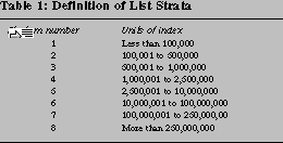
The list sample was selected in two stages. First, for cost reasons the ITF was subsetted to include only taxpayers who filed from addresses in one of the PSUs selected for the AP sample.9 Next, the remaining cases were separated into strata defined in terms of the wealth index and higher strata are sampled at a higher rate (table 1).10 The highest stratum was not sampled at all.11
As a part of the agreement with SOI, since 1989 a special approach has been taken to contacting the list sample cases. Before these cases are approached by an interviewer, they are mailed a package containing a description of the survey, and letters from the Chairman of the Federal Reserve Board and from an official at the organization conducting the survey, requesting cooperation with the survey. Also enclosed with these materials is a prepaid postcard to be returned if the individual does not wish to be interviewed.12 Taxpayers not returning the postcard are approached with the same intensity as the area-probability cases.
II.B.2 Problems with List Design
To provide motivation for some of the weighting adjustments, we summarize here some problems with the list design that are covered more thoroughly in Kennickell and McManus [1993] and Frankel and Kennickell [1995]. First, the geographic distribution of taxpayers with high values of the wealth index is very different from that of other people. In general, people who are wealthier in this sense tend to cluster more than other people, particularly in large cities. There are also significant clusters of such people in areas that are not included in the sample, and many areas in the sample with relatively high numbers of households and relatively small numbers of wealthy people. One indicator of the error in the equal distribution assumption is the fact that the survey estimate of the number of people in stratum 6 and above in the selected areas (using ITF weights adjusted by the area selection probabilities) is only 81.5 percent of the estimate obtained from the full ITF. This deviation indicates a potentially serious decrease in the efficiency of the sample. Adjustments are made by post-stratification at the weighting stage to correct the sample estimates of taxpayers in the upper strata.
There are other conceptual problems with the wealth index that may cause some observations to be classified in an incorrect stratum. However, unless these misclassifications are systematically correlated with other relationships that we care about in analysis, these problems serve only to decrease the efficiency of our estimates. In some cases there are assets (such as IRAs, Keogh accounts, antiques, artwork, etc.) that yield no regular income that would usually show up on a tax return, causing such cases to have a wealth index that is too low relative to their net worth. By stratum, the median fraction of such omitted assets ranges as high as 15 percent of assets, and the fraction is substantially higher for some cases. The assumed value of the principal residence also frequently appears inadequate. Even more troublesome is the set of rates of return that are assumed in computing the wealth index. From data reported in the survey, we know that for many businesses and some types of real estate, the income flows can be highly variable (or even close to zero for new businesses) and provide very little information about the true value of the asset. This may be less of a problem for other types of assets, but we have little information to gauge the problem.
Unlike the AP sample, which is selected as a function of a current-year characteristic, place of residence, list cases are selected based on a previous-year (or earlier) characteristics, location and level of the wealth index. Very preliminary information available from an embedded panel in the ITF reported in Kennickell and McManus [1993] suggests that incomes, which are the basis of the wealth index, are quite variable, and there is a tendency for high incomes to decline somewhat. Other support for this finding is given by Williams and Sammartino [1993]. Again, unless income variability is correlated with financial behavior, this problem is also one of sample efficiency.
One of the messiest problems with using the list frame together with the area-probability frame is the fact that the latter is based on housing units, while the former is based on tax filing units, which are individuals or married couples. A household may contain multiple filers, and the filers within a household may change between the time the returns used in the sample selection are filed and the time of the survey. The problem with having additional economic units in a selected household is that in such cases the household should have a selection probability that accounts for the possibility that any of the tax-filing units in the household could have been selected. Since nothing is known about either the filing status or the types of income reported by the additional units, we are limited in the corrections we can make. However, the data suggest that ignoring this problem may not be too serious, at least for net worth estimation. The 1992 SCF contains limited information on these units. About 18 percent (unweighted) of the households selected in the bottom wealth index stratum contained at least one economic unit besides the PEU. In the top wealth index stratum, the proportion drops to only 0.4 percent. For most cases, the ratio of the wealth held by these secondary units to the wealth of the PEU is very small: the median ratio is about 1 percent. In about 10 percent of cases, other economic units have wealth greater than that of the PEU, but this proportion drops off quickly in the higher strata.
A closely related issue is the filing status of the selected
taxpayer. If that person is married, he or she may choose to file a
joint return with a spouse or to file separately. According to the
1992 SCF, the proportion of separate filers is relatively small among
respondents in every stratum except the very top (11 percent) and the
very bottom (12 percent) strata. The overall median of the ratio of
the taxable income of the head divided by that of the spouse/partner
is 1.1. However, this figure ranges broadly over the wealth-index
strata, with the lower strata having a median close to 1, and the top
two strata having a very large median ratio. At the sample selection
stage, we assumed that in cases of separate filers, the two 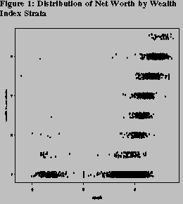 partners had identical
values of the wealth index.13 This assumption
may create some problems at the upper end of the distribution, but at
this point it is not clear what can be done in a systematic way.
However, because the number of cases involved is fairly
small--particularly in the higher strata--the bias is likely to be
correspondingly small.
Given the inefficiencies and limitations of the wealth index, one might reasonably ask how good it is as a means of stratifying cases in terms of the desired variable, net worth. In the 1992 survey, the index had only a .41 correlation with net worth, though the Spearman rank correlation--0.84--is considerably higher. As a graphical summary of the performance of the index, figure 1 shows the distribution of a transformation of net worth by wealth-index strata.14 From this picture, it is clear that the index is achieving the desired effect, even though the distinction between neighboring strata is blurred.15
III. Computation of Weights
In practice, it is not possible to compute a pure design-based weight for the entire SCF sample. To do so would require that we be able to compute the joint probability of observation under either sample frame. This calculation is inhibited by two factors. First, the representation of the AP cases within the list frame is not known. Second, there is clear evidence that nonresponse in the list frame is non-ignorable (Little [1983]) within the list sample (see Kennickell and McManus [1993]). If, as seems reasonable, nonresponse in the AP sample is similarly non-ignorable, simply assigning a list case a probability of observation under the area frame equal to that of an area case would yield biased results. The weight that we create for the 1992 SCF sample is a "post-stratification weight" (PSW) that relies to as high a degree as possible on the original probability design of the sample.16 The SCF is multiply-imputed, and each set of imputations is stored as a separate replicate ("implicate") of the data record (see Kennickell [1991]). Weights are constructed for each of the five implicates separately.
III.A. Construction of Separate Frame Weights
The construction of the weights proceeds in three steps. First, we attempt to produce the best weights for each sample separately, given the available information. Next, the separate frame weights are combined based on assumptions about the relative information content of each sample for certain domains. Finally, the combined weights are subjected to raking and other post-stratification adjustments.
III.A.1. Area-Probability Weights
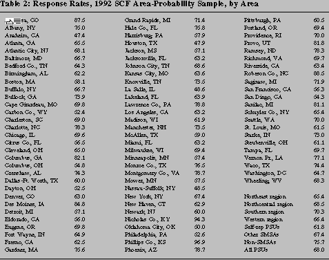
For the AP sample, table 2 gives the percent of eligible cases in each PSU that responded to the 1992 survey. Compared with the 1989 survey, the distribution of response rates in 1992 is fairly uniform.17
The information available for nonresponse adjustments in the AP sample is very limited.18 At this point, the only usable systematic information we have for the AP sample is the location of the sample cases. Thus, we are limited to nonresponse adjustments at the PSU level, implicitly assuming that nonresponse is ignorable within PSUs. The nonresponse adjustment consists of multiplying the base weight of every participating AP case in each PSU by the ratio of the number of eligible cases to the number of respondents.
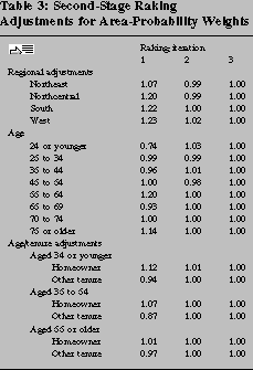
Because the AP sample is based on a 1980 frame, we would like to adjust the population figures to an exact 1992 basis.19 To accomplish this goal and to incorporate other important information about the population structure, we further adjust the population totals using three iterations of a rake based on control figures estimated from the March 1992 Current Population Survey: first the weights are adjusted to regional totals, then to fine age categories, and finally to a two-way cross of age categories and housing tenure (see table 3).20 Regional controls allow for broad population shifts. Age and housing tenure are included to capture some economic factors in the patterns of nonresponse and to ensure that these two variables, which are very important in the analysis of the data, match the best estimates available for the population.
 III.A.2. List Weights
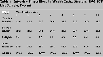
As shown in table 4, nonresponse for the list sample varies widely
over wealth index strata. Because the list frame contains a great
deal of auxiliary information on respondents and nonrespondents, we
are able to make a variety of complex adjustments for nonresponse.21 As noted in the discussion of the sample design,
the wealth index used to stratify the list sample was based on tax
data from units in existence two years earlier. By the time of the
survey, several selected units had divorced. In the event that a pair
of selected joint filers divorced during this time, a decision was
made to follow both parties, and each member of the original couple
was assigned the original ITF base weight.22
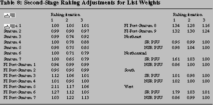
At the second level of adjustment, we perform three iterations of
a three-level raking procedure. The rake margins are totals for the
original sampling strata, for post-strata defined in terms of a
measure of financial income constructed with components of taxable
income in the ITF (table 7), and for geographic areas defined as the
four major Census regions crossed with self-representing PSU status
(table 8).23 Earlier research on nonresponse
in the SCF list sample (see Kennickell and McManus [1993]) suggests
that this measure of financial income accounts for about
three-quarters of the explanatory power of a detailed model of
nonresponse.24 The motivation at this stage is
to introduce this important variable while preserving the allocation
of the original design and further realigning the geographic
distribution of the sample, without the additional complications of
more complex model-based adjustments.25
III.A.2.a. Adjusting the Overall Population Totals for the List Weights
As noted earlier, the list frame refers to the population filing
tax returns in 1991 largely for tax year 1990, while the AP sample is
defined in terms of households in existence at the time of the survey
in 1992. We make a set of simple assumptions about the growth of the
number of list sample cases to put the list weights on the same
population basis as the AP sample.
One possibility is to allow all types of cases to grow in size by
the overall rate of growth in the number of households from 1990 to
1992 (1.7 percent). However, if the correspondence between household
growth and growth in the number of tax filers is not uniform for all
groups, this adjustment could lead to a distortion. Evidence
presented in Kennickell and McManus [1993] suggests that the alignment
of households and tax-filing units is close for the higher
wealth-index strata. In addition, these units are highly likely to
file a tax return for every year they are in existence. Thus, we
assume that the number of cases in the wealth-index strata three
through seven increase in size at the same rate as the overall
population. For the bottom two wealth-index strata, we define a
control total using the AP sample and the adjusted weights for the top
five strata. The survey asks about tax filing status for tax year
1991, which we take as a proxy for 1992 filing status. We use the
adjusted AP weights to estimate the number of households filing
returns for either the head or the spouse/partner in 1992, and the
control total for strata one and two combined is given by this total
less the number of households in stratum three and above estimated
using the adjusted weights.26 This
approach implies a uniform adjustment of 0.82 in the weights of cases
in strata one and two.
III.B. Combining Area-Probability and List Weights
At this stage in the weight development, we have our best
estimates of the nonresponse-adjusted weights for both the AP and list
samples. There are procedures that could be used to make estimates
given the two separate samples. However, much of the information that
would be needed for such calculations cannot be released. Thus, we
create a merged weight. Such a merged weight would be straightforward
if the probability of observation were known for each case under each
design. As noted earlier, this information is not available. Thus we
must make some assumptions to proceed. We develop a
post-stratification technique for this purpose.
To reduce excessive variation of the weights in some gross-asset post-strata, the weights
in post-strata 2 through 7 were truncated at the 95th percentile, and those in the first post-stratum--where the number of cases is much larger than in any of the other post-strata--were
truncated at the 99th percentile and the mass removed by truncation was spread uniformly over
all cases within each post-stratum (table 13).
IV. Construction of Bootstrap Weights
For many purposes, it is very desirable to be able to estimate
variances for statistics derived from the SCF. However, the classical
means of variance estimation (e.g., balanced repeated replication or
linearization) are not possible in the SCF, at least not without very
strong simplifying assumptions about the dual-frame design and the
nature of nonresponse. However, it is straightforward, though
somewhat more cumbersome than in classical procedures, to compute
variance estimates using bootstrap techniques.32 Briefly, we create a set of 999 bootstrap
replicates, selecting each replicate in a way that preserves important
properties of both the AP and list samples. For each of these
bootstrap samples, we compute a vector of weights using exactly the
same procedures described above for the main weight development.33
In the AP sample, we pair the non-self-representing PSUs into
pseudo-strata according to the original design of the sample, and
subdivide the self-representing areas into paired sets of segments.34 Taking each set of pairs one at a time, we
randomly select two areas with replacement and take all AP
observations in the selected areas.
Because the list and AP cases share a common geographic basis, we select the list sample
cases for each replicate from the self-representing PSUs and from the non-self-representing areas
drawn for the AP sample in the same bootstrap replicate. Given the set of all list cases in these
areas, we perform a second stage of selection. We sort the list cases into two levels: by their
wealth-index stratum numbers and by whether their original measure of size exceeded the original
sampling interval. Within each stratum, we randomly select cases with replacement from the
"certainty" and "noncertainty" cases separately. The justification for randomizing over the
certainty cases as well is to introduce some variance to proxy for nonresponse among this group.
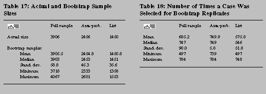
As shown in tables 17 and 18, compared with the AP sample, for the list sample there
is more variability in both the number of cases selected into the bootstrap replicates and the
number of times a given case was selected. These facts simply reflect the decisions about what
dimensions of the original design were important for sampling variance. AP cases are selected
in roughly equal-size pieces, and no subsampling is performed below the PSU level. In the case
of the list cases, there is much more variability of the number of list cases within the selected
PSUs, and we perform subselection by wealth-index strata given the PSUs. Thus, if the
assumptions made in resampling are too extreme for the list cases compared with the AP cases,
variability due to the list cases may also be relatively overstated. IV.A. Wealth Distribution
As an example of how one might use the replicate weights and the
multiply-imputed data to estimate the precision of survey estimates,
we choose the interesting and particularly difficult question of the
shape of the distribution of household net worth in 1992. The SCF is
uniquely equipped to make such an estimate since most of the survey
questions are geared toward wealth measurement, and the sample is
specifically designed to maximize the information on the high-wealth
population that holds a disproportionately large share of total
wealth.35
Table 19 provides estimates of the amounts and shares of assets, liabilities, net worth, and
income held by different percentile groups within the net worth distribution in 1992. The point
estimates suggest that 22.8 percent of all net worth was held by the top percent wealthiest
households, while the bottom 90 percent held 32.8 percent. Businesses and real estate other than
principal residences appear to figure particularly prominently in the assets of the top group. In
contrast, over half of the assets of the bottom 90 percent are accounted for by principal
residences.
SXtot = { (6/5)SX2imp + SX2samp }1/2 ,
where the imputation variance SX2imp is given by
SX2imp = (1/4) * i=1 to 5 (Xi - mean(X))2
and the sampling variance SX2samp is given by
SX2samp = (1/998) * r=1 to
999 (Xr - mean(X))2 .37
For ease of evaluation, table 19a shows the coefficient of variation for each estimate. Not
surprisingly, the variation of total assets tends to be proportionately lower than for the
components. It is interesting that overall the coefficients of variation for the top percent are
not very different than those for the other groups, and this is particularly striking in the case of
net worth. The role of imputation in these estimates of variability is substantial, but not the dominant
factor in any case. Table 19b shows the standard error with respect to imputation as a percent
of the standard error due to sampling. The standard error with respect to imputation ranges from
72.3 percent of the standard error due to sampling (for the amount of businesses held by the top
percent) to 6.3 percent (for the amount of principal residences held by the bottom 90 percent).
The practical effect is even smaller. For example, in the case of the ratio of 72.3 percent, the
total sampling error is given by
imputation sampling
error error
SXtot = (.7232 SX2samp + SX2samp).5 = 1.23 SXsamp ,
yielding a 23 percent increase over the state in which there are no missing data. In the range of
a 25 percent ratio, which is more typical, the overall standard error is inflated by only about 3
percent.
The results in table 19 stand in contrast to comparable results
reported in Kennickell and Woodburn [1992] from the 1989 SCF, which
are repeated in table 20.38 Most striking is
the decline in the point estimate of the share of total net worth held
by the top percent of the wealth distribution. In 1989 that group was
estimated to hold 28.8 percent of all net worth, with an estimated
standard error of 2.0. Even without a formal significance test, it is
obvious that the 22.8 percent estimate (with a standard error of 1.7)
is significantly different at any conventional level. Avery,
Elliehausen and Kennickell [1988] reported an estimate of 24.1 percent
for this figure from the 1983 SCF, but an estimate of sampling error
that is comparable with 1992 is not available. However, given that
the 1983 figure is within one (1992) standard error of the 1992
estimate, they are very likely not significantly different.
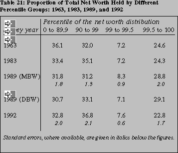
A somewhat different picture of change emerges when we look at the distribution more
broadly. For convenience, table 21 reproduces results from tables 19 and 20, together with
estimates using the "design-based" weights reported in Kennickell and Woodburn [1992], and
estimates for 1963 and 1983 from Avery, Elliehausen and Kennickell [1988]. Standard errors
are not available for 1963 or 1983, or under the design-based weights in 1989.
Over the period covered by the SCF--1983 to 1992--the fraction of net worth held by
the bottom 90 percent of the wealth distribution is estimated to vary by no more than 2.6
percentage points. Our ability to apply formal significance tests here is limited, but the 1983
estimate is within one (1992) standard error of the 1992 estimate. Moreover, the 1989 model-based weight estimate is within one (1989) standard error of the 1983 figure and within one
standard error (1989 or 1992) of the 1992 figure. Thus, it seems very reasonable to suppose that
the fraction of net worth held by the bottom 90 percent of the distribution did not change
significantly over the 1980s, and that one must look elsewhere within the top 10 percent of the
distribution to explain the changes in the share of the very top group.
The much earlier 1963 Survey of Financial Characteristics of
Consumers (SFCC) may offer some more perspective on the question of
changes in wealth concentration.39 Like the SCFs from
1983 and forward, the SFCC was directed by staff at the Federal
Reserve Board, and it used a sample drawn from tax data to provide a
better representation of the top of the wealth distribution. Although
it was not possible to apply to the SFCC the complex statistical
techniques used in the SCF, the surveys provide roughly comparable
data. Concentration estimates based on the 1963 data suggest that the
share of net worth held by the bottom 90 percent of the distribution
may have fallen over between 1963 and 1989 and begun to turn up again
in 1992. We are not able to apply formal significance tests to the
change, but based on the available standard errors, it seems likely
that at least part of this change would be judged significant in terms
of sampling and imputation error.
V. Future Research
In this paper, we have described a weighting methodology and a straightforward (though
computationally intensive) method of computing estimates of sampling and imputation error.
This work is a significant extension of earlier work reported in Kennickell and Woodburn [1992]
and Kennickell and McManus [1993]. However, there are a number of areas where the SCF
sampling and weighting procedures--which are obviously interdependent--need refinements.
Unit nonresponse in the list sample is high, and experience suggests that it is unlikely that
we can make large advances there. However, there is still good reason to believe that we can
make further progress in modeling nonresponse for this sample using frame data. Only the
pressure of time has kept us from pursing that direction here, and we fully expect to follow up
on this with the 1995 SCF. Nonresponse in the AP sample is also a potentially serious problem.
Because we have the list sample and means to adjust the list sample for nonresponse, it may not
be so troublesome if the rates of nonresponse among wealthy families in the AP sample are
similar to those we find in the list sample. However, it is well known, at least in survey folklore
if not in documented studies, that unit nonresponse is a particularly serious problem at the bottom
end of the wealth distribution. This problem affects both samples, but we have no expectation
of being able to address the problem with the list sample since it only includes tax filers and it
has complicated imperfections at that end of the wealth spectrum. To make progress with this
source of nonresponse, we have expanded the information collected for every case (interviews
and noninterviews) and we will attempt to use this information for better adjustment of the AP
sample weights in the 1995 SCF.
We know that the geographic distribution of list sample cases differs strongly from that
of the general population, and in the 1998 SCF we expect to make specific allowances for this
fact at the design stage, rather than having to impose the result through post-stratification.
Unfortunately, the necessary work for this purpose could not be completed in time fo the 1995
survey. However, additional information on changes in the AP sample frame was collected
during the administration of the 1995 SCF. This information will be used to update the frame
estimates of housing units to avoid, at least in part, the heavy reliance on post-stratification.
Changes in the SCF list sample design for the 1995 survey introduced a calibrated
approach to calculating the wealth index that serves as the basis for stratification (Kennickell and
Frankel [1995]). Our expectation is that this refinement will reduce the variance of list sample
weights within gross asset groups, and thus lessen our dependence on ad hoc weight truncation.
In the selection of the bootstrap samples used in the construction of the replicate weights,
we use only what we believe are the important dimensions of the original sample selection. This
procedure takes no direct account of nonresponse. However, as we know even from the simple
tables in this paper, nonresponse varies systematically in several dimensions. In the future, we
expect to develop a resampling method that takes at least some account of the fact that not all
cases within a cell have equivalent probabilities of observation. It might be possible to take
account of these differences by using additional models, by using categories of the sort we have
used here for post-stratification (e.g., financial income cells), or even by taking a function of the
main weight as a size measure for cases within selection cells.
Throughout this paper, we have made almost no mention of nonsampling error other than
imputation error. This is appropriate given that this paper is concerned with weights and
associated subjects. However, we do not want to leave the reader with the impression that other
sources of error are unimportant. There is explored territory concerning other measurement error
(e.g., see Sudman, Bradburn, and Schwarz [1996]), and huge unexplored territory. It is clear to
practitioners that interviewer effects, mode effects, and similar factors play a large part in the
statistical reliability of the final data. At this point, our ability to measure such factors is still
relatively small. For the future, it is important to think of the surveys as integrated statistical
processes, to apply measurement and feedback wherever possible, and to try to solve agency and
moral hazard problems by motivation and incentives where actions are unobservable or partially
unobservable--particularly in the case of interviewer behavior.
BIBLIOGRAPHY
Avery, Robert B., Gregory E. Elliehausen, and Arthur B. Kennickell [1988] "Measuring Wealth
with Survey Data: An Evaluation of the 1983 Survey of Consumer Finances," Review of
Income and Wealth (December), pp. 339-369.
Frankel, Martin and Arthur B. Kennickell [1995] "Toward the Development of an Optimal
Stratification Paradigm for the Survey of Consumer Finances," paper presented at the
1995 Annual Meetings of the American Statistical Association, Orlando, FL.
Greenberg, Daphne [1983] "An Estimation of U.S. Family Wealth and its Distribution from
Micro-Data," Review of Income and Wealth (March), pp. 23-44.
Internal Revenue Service [1992] "Individual Income Tax Returns, 1990."
Kennickell, Arthur B. [1991] "Imputation of the 1989 Survey of Consumer Finances: Stochastic
Relaxation and Multiple Imputation," 1991 Proceedings of the Section on Survey
Research Methods, Annual Meetings of the American Statistical Association, Atlanta, GA.
__________ and Douglas A. McManus [1993] "Sampling for Household Financial Characteristics
Using Frame Information on Past Income," Proceedings of the Section on Survey
Research Methods, 1993 Annual Meetings of the American Statistical Association, San
Francisco, CA.
__________ and Martha Starr-McCluer [1994] "Changes in Family Finances from 1989 to 1992:
Evidence from the Survey of Consumer Finances," Federal Reserve Bulletin (October),
pp. 861-882.
__________ and R. Louise Woodburn [1992] "Estimation of Household Net Worth Using
Model-Based and Design-Based Weights: Evidence from the 1989 Survey of Consumer
Finances," mimeo Board of Governors of the Federal Reserve System.
Kish, Leslie [1965] Survey Sampling, John Wiley, New York.
Little, Roderick J.A [1983] "Chapter 21: The Ignorable Case" and "Chapter 22: The nonignorable
case," in Incomplete Data in Sample Surveys, New York: Academic Press.
Projector, Dorothy S. and Gertrude S. Weiss [1966] "Survey of Financial Characteristics of
Consumers," Board of Governors of the Federal Reserve System.
Sitter, R.R. [1992] "A Resampling Procedure for Complex Survey Data," Journal of the
American Statistical Association, 87(419), pp. 755-65.
Sudman, Seymour, Norman M. Bradburn, and Norbert Schwarz [1996] Thinking About Answers,
Jossey-Bass, San Francisco.
Williams, Roberton and Frank Sammartino [1993] "Income Mobility of the Rich: Some
Preliminary Findings," paper presented at the 1993 Annual Meetings of the American
Statistical Association, San Francisco, CA.
* Part
of the work on this paper was done while Kennickell was a visitor at
the Center for Economic Research (CentER) at Tilburg University in the
Netherlands. The authors are grateful to Herman Camphuis, Arie
Capteyn, Gerhard Fries, Barry Johnson, Myron Kwast, and Martha
Starr-McCluer for comments and support, and to James Faulkner, Todd
King, and Diane Whitmore for research assistance. The opinions
presented here are the responsibility of the authors alone and do not
necessarily reflect the views of the Board of Governors of the Federal
Reserve System, Freddie Mac, or the Internal Revenue Service. All
remaining errors are the responsibility of the authors.
| return to text
1 There
is an earlier series of surveys done by the University of Michigan
with sponsorship of the Federal Reserve. However, these surveys were
largely intended for purposes other than the measurement of the
distribution of financial characteristics. The earliest
U.S. prototype of a survey like the SCF was the Survey of Financial
Characteristics of Consumer, conducted by the Federal Reserve in 1963
with a follow-up in 1964 (see Projector and Weiss [1966]). | return to text
2 In most households, the
economically dominant person or couple is obvious. In a household
containing only one person or couple that own or rent the dwelling,
the PEU consists of this person or that couple and all people
financially interdependent with this person or couple. Where more
than one person not related or living as partners own or rent the
dwelling, the person nearest age 45 is selected along with that
person's spouse or partner (where relevant) and all other persons
financially interdependent with that person (or that
couple). | return to text
3 Although an area-probability
sample based on the 1990 Census data was just available at the time
the sample was to be selected, the cost of listing many new segments
combined with the desirability of retaining as many as possible of the
experienced interviewers in the old primary sampling units argued for
using the older sample. | return to text
4 The construction of the ITF is
described in detail in "Individual Income Tax Returns, 1990." As a
sample, the ITF has statistical properties that should be
considered. However, for the representation of higher-income cases,
which is the main reason for our using the ITF, sampling rates from
the universe of taxpayers are sufficiently high that sampling error
for this group is relatively unimportant. | return
to text
5 For purposes of the SCF list
design, all returns from foreign addresses (including APO addresses)
were deleted from the frame. Where there were multiple returns from
one taxpayer, only the most recent return was
retained. | return to text
6 For example, it a taxpayer
reports $100 in interest income and the rate of interest were assumed
to be 10 percent, then the value of the asset that generated the
income would be estimated to be $1,000. This technique has been
commonly used in economics (see, e.g., Greenberg [1983]). Recent
evidence (see Frankel and Kennickell [1995]) suggests that the
relationship is quite noisy. | return to
text
7 Clearly, there is no direct
logical justification for the absolute value function if we are
literally attempting to estimate wealth. There are actually few cases
with significant negative income flows at this level and there was a
presumption that people with large negative income must have had
substantial assets to be able to sustain a negative income. | return to text
8 If a sample couple filing a
joint return had divorced by the time they were contacted, they were
assigned a new value of the wealth index given by
WINDEX(div)=(WINDEX(mar)-home equity)/2+home equity for use in
nonresponse and other post-survey weight adjustments. | return to text
9 One important qualification in
the use of this file is that the address that is reported in the tax
data may not be that of the person whose name is on the return.
Although the IRS requires filers to use their own mailing address, it
appears that in some cases the address may be that of an accountant,
lawyer, or other tax-preparer or agent. |
return to text
10 For confidentiality reasons,
the exact sampling rates cannot be revealed.
| return to text
11 The total number of cases in
the highest stratum is very small, the probability of obtaining an
interview is very small, and the likelihood of other problems is
large. Even though the top group probably controls a large amount of
assets, the fraction of net wealth held by the group is relatively
small and might be better approximated from other sources, such as
Forbes. | return to text
12 In 1983, a similar procedure
was followed, except that the postcard was to be returned only if the
person agreed to be interviewed. As would be expected, response rates
for the list sample in 1983 were dramatically lower--only about 10
percent of the sample agreed to participate.
| return to text
13 The effect of this assumption
is that we divide their weights by 2 at the sample selection stage to
account for the multiple occurrence of the family. | return to text
14 The data reported in these
charts is based on imputed data from the participants in the 1992 SCF,
and thus take no account of the unit nonresponse discussed in the next
section. Net worth is displayed on the horizontal axis using a
convenient logarithmic transformation of the data: For strictly
negative values the value is the negative of the base-ten logarithm of
the absolute value of the number, and for numbers greater than or
equal to zero, the figure is equal to the base-ten logarithm of the
maximum of one and the value of the variable.
| return to text
15 The data used in the plot for
this paper are also blurred for confidentiality reasons. However, the
same pattern is evident in the unaltered data. | return to text
16 For the 1989 SCF, we also
computed a more model-based weight. As it turned out, this weight
added a great deal of complexity to the weight construction, but did
not produce interesting differences from the PSW. | return to text
17 See Kennickell and McManus
[1993] for the rates in both years. The difference is a result of a
conscious investment of interviewer resources intended to reduce the
component of estimation variance due to variation in the weights for
the AP sample. | return to text
18 Interviewers recorded some
data on neighborhood characteristics of all the area
cases--respondents and nonrespondents. However, there are missing
values of this information for some cases. Moreover, general
experience in other surveys is that interviewers are not able to make
analytically usable distinctions about types of housing structures and
neighborhoods. These variables are currently under investigation and
may be used in later adjustments. We expect to develop more useful
measures for the 1995 SCF. | return to
text
19 In principle, additions of
addresses to the 1980 frame (estimated as the difference between the
final number of lines listed in a segment and the Census figure)
should provide an estimate of the number of housing units in 1992.
Unfortunately, the methodology was not in place at the time of that
survey to capture this additional information. The 1995 SCF will
employ added addresses in this way. | return
to text
20 If anyone in a household
owned any part of the dwelling or the ground on which it was located,
the unit was treated as a homeowner. | return
to text
21 Use of SOI data for purposes
of nonresponse adjustment is governed by contract agreements between
the Federal Reserve, the Statistics of Income Division of the IRS, and
NORC. Under the terms of these agreements, there are strict limits
imposed on the use of tax information, and all information produced as
a result of using tax data are subjected to a thorough review to
protect the privacy of survey respondents and nonrespondents. | return to text
22 The base input for the list
weight is the inverse of the probability of selection, which is the
product of the probability of selection into the SOI sample (adjusted
for filing status as discussed earlier), the probability of selection
of the areas in the AP sample, and the sampling rate within the list
sampling strata (with adjustments for cases with size measure greater
than the sampling interval). | return to
text
23 Financial income includes
income reported on the tax return for taxable and nontaxable interest,
and dividends. | return to text
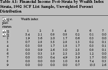
24 A table in the appendix gives
the unweighted joint distribution of the respondents in the list
sample over wealth index strata and financial income post-strata. | return to text
25 Because there is relatively
large difference on average between nonresponse in self-representing
PSUs and that in non-self-representing PSUs, we impose the more
detailed geographic factor here. The use of these terms is also
supported by the results of Kennickell and McManus [1993]. | return to text
26 Some adjustments to the
survey data were made to determine tax filing status for respondents
in 1991. The survey requested this information directly. In cases
where a respondent had not yet filed a return but expected to do so
later, the survey also requested this information. AP cases with more
than $50,000 in financial assets and all list cases were assumed to
have filed a tax return regardless of what they reported to the direct
question. | return to text
27 The survey estimates that
13.7 percent of households did not file a tax return in 1991. Where
the filing status is missing in the survey, we use imputed values. | return to text
28 Where necessary, imputed data
were used in this calculation. | return to
text
29 Formally, the merging is as
follows: In post-stratum i, let Nia = weighted number of AP
cases, Nil = weighted number of list cases, nia
= the unweighted number of AP cases, nil = the unweighted
number of list cases, and let Ris =
(nis/Nia)/[(nia/Nia) +
(nil/Nil)] for s={a,l}. Then for case j from
sample s in post-stratum I, COMBINDED_WGTj = Ria
* AP_WGTj + Ril * LIST_WGTj , where
AP_WGTj is the nonresponse-adjusted AP weight (equal to
zero for list cases), and LIST_WGTj is the
nonresponse-adjusted list weight (equal to zero for AP cases). | return to text
30 This decision implicitly
reflects an assumption that the best estimate of the number of cases
in this group is determined by the list sample. Given the high
correlation of indicators of wealth and nonresponse, it is highly
likely that any such estimates based on the AP sample would be
strongly biased. | return to text
31 All the post-stratification
and raking control totals for the adjustment of post-strata one and
two are derived from CPS data less the totals for cells estimated with
the adjusted weights for higher post-strata and for the nonfilers. | return to text
32 See Sitter [1992] for a
discussion of variance estimation using bootstrap techniques. | return to text
33 Replicate weights are
created only for the first implicate. |
return to text
34 These are the groupings one
would use in performing a BRR estimate of variance using the AP sample
alone. | return to text
35 Note that the net worth
measure considered here does not include the present value of Social
Security benefits, future benefits from defined-benefit pension plans,
or measures of human capital. Ongoing research on the first two of
these issues will provide appropriate data for the inclusion of these
factors in future calculations. | return to
text
36 The figures shown in the memo
items for the number of observations and the minimum net worth in the
group also vary with sampling and imputation. For simplicity, these
figures are shown only for the first implicate. | return to text
37 For the imputation variance,
the mean function is taken with respect to all five implicates. For
simplicity, we have computed bootstrap weights only for the first
implicate. Thus, for the sampling variance, the mean function is
taken with respect to all 999 bootstrap replicates. | return to text
38 The Kennickell and Woodburn
figures were estimated with a set of model-based weights they
computed. We choose that set here rather than the more design-based
weights because standard errors are only available for the model-based
weights. The techniques reported in the creation of the weights in
this paper are a refinement of the approach taken in the calculation
of these 1989 model-based weights. | return
to text
39 See Projector and Weiss
[1966] for additional information on the SFCC. | return to text
40 Projector and Weiss [1966]
report an estimate of 0.76 from the 1963 SFCC. | return to text
41 As another indicator of the
changes in the distribution of net worth, median (mean) net worth
adjusted to 1992 dollars using the CPI, is estimated to be $33,700
($107,000) in 1963, $48,300 ($168,700) in 1983, $51,500 ($197,200) in
1989, and $48,700 ($185,100) in 1992. |
return to text
 A small
number of cases have net worth much greater or smaller than other
cases in their original sampling strata--that is, misclassification
appears to be a problem. Some such cases may have had a change in
household composition since the time of the tax returns on which the
sample is based, some may have had unusual income in that year, and
for some the wealth index may be inadequate for other reasons. A
number of possible adjustments are possible. For simplicity, we
decided for purposes of weighting to reassign the initial weights of
cases that had unusually high or low values of gross assets within
each stratum. Cases with a level of gross assets exceeding the 90th
percentile of the next highest wealth index stratum, or lying below
the 10th percentile of the next lowest stratum, are assigned the
median weight for that neighboring cell. Table 5 shows the number of
affected cases by wealth index stratum.
 The weight is then adjusted in several stages using control data from the entire ITF (not
just the cases in the selected PSUs). An initial adjustment is made for nonresponse by wealth
index strata and geographic location. The intention here is to align the sample to the original
frame in a way comparable to what is done for the AP adjustments and to provide a preliminary
realignment of the weights to account for some rough geographic distortions. The adjustment
factors are shown in table 6.
 First, AP
cases that did not file a 1991 tax return are given their
nonresponse-adjusted weight computed as above.27 Second, the remaining cases are divided into
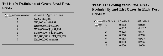
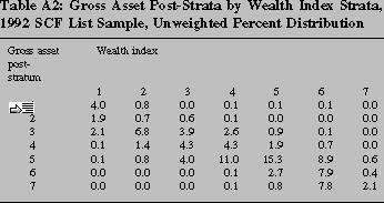
seven post-strata defined in terms of gross assets (see table 10).28 There are many possible alternatives to gross
assets, including possibly an index number created as a weighted
average of several concepts. We have found that using gross assets
categories in this way yields good weights for most estimation
appropriate for the SCF. Because each sample purports to represent
the same population of tax-filers, we combine AP and list cases within
each of these post-strata scaling each weight its weighted
contribution to the number of cases in each post-stratum (table 11).29 We then adjust the weighted counts to maintain
comparability with external figures (table 12). Post-strata three and
above are adjusted to control totals estimated from the list sample
alone.30 Control totals for the first two post-strata are
computed as a residual of the CPS estimate of households less the
totals for the higher post-strata and the number of nonfilers.
 III.C. Final Adjustments
 Because we
have no systematic external information on the demographic
characteristics of wealth households and we wish to minimize the
variation in the weights of such households, we make no further
adjustments to the weights of cases in post-strata three and higher.
For the remaining cases, there is good external information. We
subject cases in post-strata one and two to a final round of
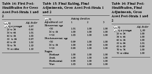
post-stratification and raking in three steps. First, the weights are
post-stratified by the fine age categories (table 14).31 Next, these cases are subjected to three
iterations of a rake from homeownership/coarse age categories to
region categories (table 15). Finally, these weights are
post-stratified to finer age categories (table 16). Separate weights
are created for each implicate.
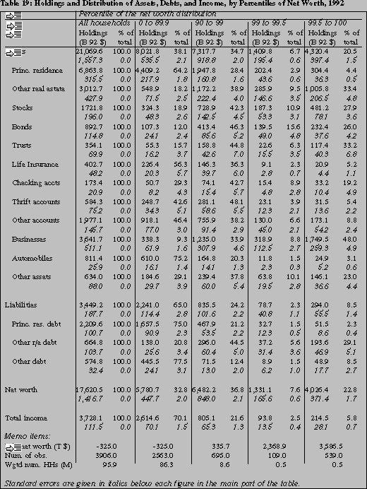
 The table also shows
the standard error of each estimate attributable to sampling and
imputation combined.36 The standard error for
statistic X is estimated as:
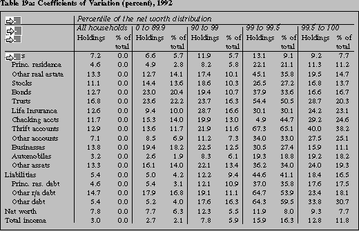
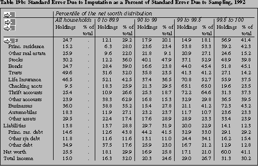 Figure 2 shows a kernel density plot of the distribution over the 999 bootstrap replicates,
of the share of net worth held by the top of one percent of the net worth distribution in 1992.
Because we did not construct weights for all implicates, we are unable to display the imputation
and sampling variation on the same chart. As is evident from the picture, the mass of the
distribution is very tightly clustered between about 20 and 24 percent.
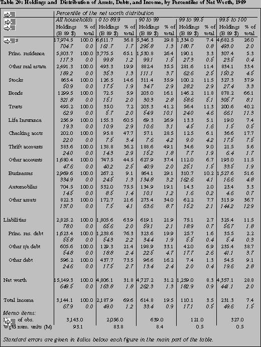 The change between 1989 and 1992 in the point estimate of the share held by the top
percent appears to be the result of an 8 percent decline in the nominal level of the holdings of
that group while the total for all households rose by about 17 percent. There were also sizable
declines in the top group's holdings of bonds, trusts, and 'other' assets. This drop in the wealth
of this group may reflect directly or indirectly the lingering effects of the 1991-92 recession,
falling prices for real estate, the rise in business failures, or a cooling in the markets for some
financial assets and for art.
 Another
distributional measure of net worth is the Gini coefficient, defined
as one minus twice the area under the Lorenz curve (the cumulative
percentile distribution of net worth plotted against the corresponding
percentile distribution of households). In the case that all assets
are distributed equally, the Lorenz curve is a diagonal line and the
Gini coefficient is equal to zero. In the case that all net wealth is
held by one household, the Gini coefficient is equal to one. Using
data from the 1983 SCF, Avery, Elliehausen, and Kennickell [1988]
reported a value of 0.777 for the Gini coefficient. From the 1989 SCF
data, Kennickell and Woodburn [1992] estimated that the value had
risen significantly to 0.793 with a standard error due to sampling and
imputation of 0.011. Using the 1992 SCF data, we find that the point
estimate has fallen to the intermediate value of 0.782 with a standard
error of 0.011 for the 1992 estimate. Both the 1983 and 1989 values
are within a single standard error.40 Thus, according to
this measure, the overall direction of change in the distribution of
wealth since 1983 is statistically ambiguous.41
Top of page
Home | Surveys
| OSS |
SCF index
To comment on this site, please fill out our feedback form.
Last update: December 1, 2000, 5:00 PM