Skip to: [Printable Version (PDF)] [Bibliography] [Footnotes]

Finance and Economics Discussion Series: 2007-57 Screen Reader version ^♣

Financial Market Perceptions of Recession Risk

Thomas B. King, Andrew T. Levin, and Roberto Perli^*¹

Keywords: Recession forecasting, yield curve, term spread, credit spread

Abstract:

Over the Great Moderation period in the United States, we find that corporate credit spreads embed crucial information about the one-year-ahead probability of recession, as evidenced by both in- and out-of-sample fit. Furthermore, the incidence of "false positive" predictions of recession is dramatically reduced by utilizing a bivariate model that includes a measure of credit spreads along with the slope of the yield curve; indeed, these bivariate models provide much better forecasting performance than any combination of univariate models. We also find that optimal (Bayesian) model combination strongly dominates simple averaging of model forecasts in predicting recessions.

Introduction

Central banks watch financial markets closely, at least in part because financial data may embed valuable signals about the state of the economy and risks to the macroeconomic outlook. For example, conventional wisdom holds that negative term spreads--that is, a downward-sloping yield curve--generally reflect an elevated risk of recession over the subsequent year.² Furthermore, a long tradition has emphasized the extent to which a widening of credit spreads--that is, the difference in yields between low- and high-grade securities--can provide advance warning of a deterioration in macroeconomic conditions.³

However, recent research has cast significant doubt on the extent to which statistical models can provide robust signals in forecasting economic growth or assesssing the near-term risk of recession. For example, several studies have documented a weakening link in the relationship between term spreads and economic activity over the past couple of decades.⁴ More generally, the analysis of Stock and Watson (2003)--henceforth referred to as SW03--has highlighted the unsatisfactory performance of statistical models in forecasting GDP growth, although their study focused on univariate models and did not include any measures of corporate credit spreads.

In this paper, we perform a systematic comparison of statistical models of U.S. recession risk over the Great Moderation period. In particular, we consider monthly data for the period 1988 to 2007 for 54 different financial-market variables, including all of the series considered by SW03 as well as a variety of corporate credit spreads and several other distinct measures of market liquidity. Furthermore, we examine the entire space of bivariate statistical models to determine whether any of these models can provide a substantial improvement in the Bayesian information criterion or out-of-sample forecasting performance of the best univariate models. Finally, we investigate the benefits of combining individual model forecasts via either simple unweighted averaging or Bayesian model averaging (which places relatively greater weight on models with higher posterior probability).

Our analysis indicates that corporate credit spreads embed crucial information about the one-year-ahead probability of recession, as evidenced by both in-sample fit and out-of-sample forecasting performance. Furthermore, the incidence of "false positive" predictions of recessions is dramatically reduced by utilizing a bivariate model that includes both a credit-spread measure and a term-spread measure. In 2006, for example, the yield curve was generally flat or inverted and hence models based solely on this variable signaled an alarmingly high probability of recession, whereas our data-preferred bivariate model is consistent with survey evidence indicating that financial-market participants perceived a very small risk of recession.⁵

Moreover, we find that Bayesian model averaging produces results far superior to simple model averaging in our out-of-sample forecasting exercises, in contrast to some previous studies that have found it to be inconsequential or even counterproductive. Because a large proportion of the models we consider turn out to have no meaningful forecasting ability, simple model averaging swamps the predictive power of the few informative models with overwhelming amounts of noise. On the other hand, because the models that fail at out-of-sample forecasting also generally have poor in-sample fit, Bayesian model averaging assigns them relatively little weight. The Bayesian model average thus discriminated quite strongly between the 2001 recession and the subsequent expansion, while the simple model average produced only slightly higher probabilities prior to the recession than afterwards.

We begin the sample in 1988 in light of the evidence for a structural break in term-spread models mentioned above, as well as for practical considerations of data availability and reliability prior to the mid-1980s. However, there are also good economic reasons to limit attention to a relatively recent sample. The well known drop in real-side volatility that began in the 1980s--the "Great Moderation"--appears to have involved a decline in the frequency and duration of recessions, which is likely to have altered reduced-form forecasting relationships.⁶ Furthermore, financial markets developed at an unprecedented pace during this time, giving market access to a much larger class of investors and providing those investors increasingly diverse ways to place bets on their perceptions of the economic outlook. Thus, market signals today are likely to reflect a different set of factors than they did twenty years ago. Although beginning the sample in 1988 limits us to only sixteen recession-month observations, this turns out to be sufficient to draw strong statistical conclusions about which variables are important.

The paper proceeds as follows. The following section lays out the basic logit model that we consider and discusses our approach to model comparison. Sections 3 and 4 discuss the results for the univariate and bivariate cases, respectively. Section 5 considers issues of model and parameter uncertainty, including computations of posterior probabilities that the various regressors enter the model and our model averaging exercises. Section 6 offers some conclusions.

2. Methodology

We follow Estrella and Trubin (2006) and others in modeling the probability that the economy will be in a recession exactly twelve months ahead, conditional on a vector of currently observable explanatory variables x $_{t}$ :

(1) $P_m \left( {{\rm {\bf x}}_t ;{\rm {\bf\theta }}_m } \right)\equiv P\left[ {R_{t+12} =1\,\left\vert {\,{\rm {\bf x}}_t } \right.} \right]=\lambda \left( {{\rm {\bf {x}'}}_t {\rm {\bf\theta }}_m } \right)$

where $_{s}$ is a dummy indicating a recession in month , $\lambda$ (.) is the logistic function, and $\theta$ $_{m}$ is a vector of parameters defined on the space $\Theta$ $_{m}$ . The subscript indexes different possible models, which, for our purposes, is simply defined by zeros in different positions among the elements of $\theta$ (or different choices of variables in x). Given a maximum-likelihood (ML) estimate of the parameters $\theta$ $_{m}$ ^*, the usual point estimate of $_{m}$ in any period is computed as $\lambda$ (x $_{t}$ $\prime$ $\theta$ $_{m}$ $^{\ast })$ .

Two alternatives to this basic model that are popular in the literature are (a) to use a probit, rather than a logit function, and (b) to model the cumulative probability over the twelve-month period--i.e., the probability of being in a recession at any time over the next year. The choice between logit and probit makes very little difference in the outcome of these models. The choice of whether to examine cumulative or marginal probabilities can make a difference, although we found qualitatively similar results for our sample when considering cumulative models. We focus on the one-year-ahead specification in equation (1) for ease of interpretation and to avoid introducing serial correlation through an overlapping dependent variable.

Our general approach to comparing various logit models of recessions builds on work by Estrella and Mishkin (1998) and, recently, by Wright (2006). In making these comparisons, we focus on Bayes factors. Let X $\equiv$ {x $_{1}$ , x $_{2}$ , ..., x $_{T}$ } denote the time series of the explanatory variables and R $\equiv$ { $_{13}$ , $_{14}$ , ..., $_{T+12}$ } be the series of recession dummies. For two competing models and (not necessarily nested) with parameter vectors $\theta$ $_{a}$ and $\theta$ $_{b}$ , the Bayes factor is defined as

(2) $B_{b,a} \equiv \frac{\mu _b \left( {{\rm {\bf R}}\,\left\vert {\,{\rm {\bf X}}} \right.} \right)}{\mu _a \left( {{\rm {\bf R}}\,\left\vert {\,{\rm {\bf X}}} \right.} \right)}$

where $\mu$ $_{m}$ is the marginal likelihood of model ,

(3) $\mu _m \left( {{\rm {\bf R}}\,\left\vert {\,{\rm {\bf X}}} \right.} \right)=\int\limits_{\Theta _m } {L_m \left( {{\rm {\bf R}}\,\left\vert {\,{\rm {\bf X}},\,{\rm {\bf\theta }}_m } \right.} \right)\pi _m \left( {{\rm {\bf \theta }}_m } \right)d{\rm {\bf\theta }}_m }$

and $_{m}$ and $\pi$ $_{m}$ are the likelihood function and prior parameter distribution, respectively, for model . Within each model, we specify diffuse priors for the parameters, so that the posterior distribution is determined by the likelihood function. For the logit models that we consider, the likelihood functions are

(4) $L_m \left( {{\rm {\bf R}}\,\left\vert {\,{\rm {\bf X}},\,{\rm {\bf\theta }}_m } \right.} \right)=\prod\limits_{t=1}^T {\frac{\exp \left[ {R_t {\rm {\bf {\theta }'}}_m {\rm {\bf x}}_t } \right]}{1+\exp \left[ {{\rm {\bf {\theta }'}}_m {\rm {\bf x}}_t } \right]}}$

Although the likelihood function in (4) can be computed analytically for any given value of $\theta$ $_{m}$ , the integral in equation (3) cannot. Under normality, the log of this integral is proportional to the commonly used Bayesian Information Criterion:

(5) $BIC_m =-2\ln L_m \left( {{\rm {\bf R}}\,\left\vert {\,{\rm {\bf X}},\,{\rm {\bf\theta }}_m \ast } \right.} \right)+K_m \ln T$

where $_{m}$ is the number of parameters in model .⁷ The BICs forms the basis for our in-sample model comparison. We compute these measures for each of the univariate and bivariate logit models discussed below, using monthly financial data from February 1988 through April 2006 (with R spanning February 1989 through April 2007).

We also perform (pseudo) out-of-sample tests. It is of interest to know both how well the models do in predicting recessions and how well they do in predicting expansions--that is, their type-I and type-II errors. We thus consider two test periods: (1) the 2001 recession, estimating the model on financial data through April 2000, and (2) the post-2001 expansion, estimating on data through November 2000. In general, a successful model should generate high recession probabilities in the first period and low probabilities in the second period.⁸

3. Univariate Models

We first examine the performance of financial variables one at a time. The list of 54 variables we consider appears in the first column of Table 1. The list includes all of the financial variables used by SW03, as well as spreads on 5- and 10-year corporate bonds with various credit ratings. We also include three other variables that are only available since the mid-1980s--the spread between on- and off-the-run Treasury notes (a measure of market liquidity) and option-implied volatilities on the S&P 500 and the 10-year Treasury rate.⁹ Following SW03, we transform the variables in various ways. First, for many of the nominal quantities, we deflate by a measure of inflation expectations from the Survey of Professional Forecasters, matched to the closest relevant maturity.¹⁰ Second, depending on the time-series properties of the variable, we consider logs, first differences ( $\Delta )$ , percentage changes (% $\Delta )$ , or log second differences (% $\Delta$ $^{{\rm y}})$ .

The BIC produced by each univariate logit model is shown in the second column. (For comparison, as shown in the last row, the BIC produced by a model with no regressors--i.e., a constant probability--is 121.0.) The two models ranked highest by this criterion are those based on the AA 10-year and AA 5-year credit spreads. Beyond these, models based on various term spreads have BIC's that are moderately higher. All of the other variables perform relatively poorly as univariate forecasters. The third column shows the Bayes factor for each model (using the BIC approximation), relative to the top model. Taking these numbers literally, the AA 10-year model is 5,000 times as likely to be "correct" as the best of the term-spread models, and over 1 million times as likely as most of the other models in the table.

The final two columns of the table report the results of out-of-sample tests. Of all of the variables, the 10-year AA spread produced the highest out-of-sample recession probability for the months in 2001 when a recession actually occurred. Several of the other credit spreads also yielded average probabilities of over 50% during this time. Meanwhile, most term spreads produced recession probabilities between 20 and 40 percent. On the other hand, most of the credit spreads also gave out-of-sample recession probabilities well above the unconditional probability of 10.4% during the post-2001 expansion, while most interest rates and term spreads gave quite low probabilities.

Figure 1 provides some further insight into the relative performance of credit and term spreads over this sample by plotting the in-sample recession probabilities produced by the lowest-BIC model of each type. The horizontal line indicates the unconditional recession probability of 7.3 percent. The relatively poor performance of the term spread (the dashed line) is driven primarily by three episodes. First, although the yield curve did invert prior to the 1990-91 recession, its most dramatic dip was in March of 1989, too far in advance of first official recession month, which occurred in August of the following year.¹¹ By contrast, the credit spread (the solid line) began rising precisely in August 1989. The second episode occurs in 1997-98, a period in which the yield curve was flat, producing recession probabilities of over 20% for several months in a row. Meanwhile, credit spreads remained quite low, except for a brief spike following the collapse of Long Term Capital Management in October 1998. Finally, toward the end of our sample the yield curve again inverted, even as corporate spreads remained at historic lows. Since no official recession had materialized by April 2007, this represents a failure of the term-spread model.

It is also instructive to consider some models that perform even less well. The solid line in Figure 2 gives the predictions of the ten-year high-yield credit spread. Junk-bond spreads frequently receive attention in the press because fragile firms may be especially sensitive to economic and financial deterioration. However, as the graph indicates, this sensitivity may also lead to false positives--notably, during the turmoil of 2002 and 2003, a period of financial turmoil in the wake of scandals at Enron and elsewhere. The dotted line in the graph presents the predictions of the worst-performing model, which uses the second difference of log silver prices. The recession probabilities generated by this model are nearly indistinguishable from the constant-probability case. The consideration of such models will dampen the simple model-average forecasts (but not the optimally weighted forecasts) we construct below.

We note, however, that even the best credit spreads, by themselves, are not perfect predictors. In addition to the spike in 1998, the AA spread produces some false positives in the 2002-03 period. In other words, while term spreads may ignore important information about default risk, credit spreads may be overly sensitive to financial-market noise that is not necessarily linked to macroeconomic fundamentals. Presumably, information from both sources is potentially useful. This is precisely our motivation for considering bivariate models in the following section.

4. Bivariate Models

In light of the recent difficulties the term-spread model has had, some research has suggested that additional variables may more fully capture market perceptions. Most of this work has focused on other aspects of the yield curve itself. For example, Hamilton and Kim (2002) decompose the yield curve into components due to short rates and interest-rate volatility, and Wright (2006) examines models including inflation, interest-rate levels, and term premia. In general, accounting for the level, in addition to the slope, of the yield curve adds significant forecasting power for recession models. On the other hand, SW03 conclude that adding financial variables to the term spread does not significantly enhance its success in forecasting GDP growth. Our exercises below build on these approaches but consider a more comprehensive list of possible financial factors.

Our 54 variables offer a total of 1,431 possible bivariate models. Of these, the 25 models that rank highest by BIC are presented in Table 2. All of these models dominate even the best-performing univariate model. The best of the bivariate models, which includes the AA 5-year credit spread and the 2- to 10-year term spread, is over half a million times more likely to have produced the data than the model with the AA 10-year spread alone. The solid line in Figure 3, which plots the recession probability generated by this model, shows why this is the case. The bivariate model produces in-sample probabilities of around 90 percent for the two recessions, and its false positives are minor. Note that this is a considerably different picture than that which would be provided by a simple averaging of the two corresponding univariate models, as can be seen qualitatively by comparing Figure 1. Thus, the interaction between the term and credit spreads appears to matter.

The bivariate models also do a better job in terms of out-of-sample predictability. All of the models in Table 2 would have predicted the 2001 recession with greater than 50 percent probability, and most would have given probabilities of over 90 percent. During the expansion, nearly all of these models would have produced recession probabilities of less than 10 percent, with several producing less than 5 percent. Again, the models including both term and credit spreads generally do the best job in the out-of-sample tests.

5. Model and Parameter Uncertainty

From a Bayesian perspective, the marginal likelihood of each model can be used to infer the probability of that model having generated the data. In this section, we exploit this idea to quantify the probabilities of different types of models and to produce optimally weighted (Bayesian) forecasts. The weights are constructed as

(6) $w_m =\frac{p_m \exp \left[ {{-BIC_m } \mathord{\left/ {\vphantom {{-BIC_m } 2}} \right. \kern-\nulldelimiterspace} 2} \right]}{\sum\limits_{k=1}^M {p_k \exp \left[ {{-BIC_k } \mathord{\left/ {\vphantom {{-BIC_k } 2}} \right. \kern-\nulldelimiterspace} 2} \right]} }$

where $_{m}$ is our prior probability for model , discussed below. Given these weights, we can combine the posterior distributions produced by the various models and summarize their features.

5.1 Priors

These exercises require us to specify prior probabilities $_{m}$ across models. (These were not necessary to compute the Bayes factors discussed above.) It is tempting to specify a prior that that each of the possible models is equally likely, but this would implicitly give more prior weight to the bivariate models (which are far more numerous). Similarly, certain types of variables--e.g., credit spreads--are overrepresented among our candidate regressors, so weighting all models equally would implicitly give high weight to such variables.

To avoid stacking the odds in this way, we adopt a hierarchical prior across models that incorporates, first, equal probabilities of bivariate versus univarite models; second, uniform beliefs over whether different types of variables enter the model; and, third, uniform beliefs over which variables enter within each type. Specifically, we use equal probabilities that at least one of each of the following types of variables enters the model (non-exclusively): a credit spread, a term spread, a measure of the level of interest rates, a measure of the change in interest rates, a measure of commodity-price levels or changes, and one of the remaining variables. We then assign equal probability to each variable within each of these groups. Table 3 summarizes these priors for the univariate and bivariate models considered separately, and for all of the models considered jointly.

5.2 Posterior Probabilities of Regressors

The posterior probability of each variable $_{i}$ entering the model with a non-zero coefficient is computed as

(7) $P\left[ {\theta _i \ne 0} \right]=\sum\limits_M {w_m \delta _m \left( {\theta _i } \right)}$

where $\delta$ $_{m}$ ( $\theta$ $_{i})$ is an indicator function that takes the value of 1 if $\theta$ $_{i} \quad \ne$ 0 in model and 0 otherwise. These probabilities are reported in the "posterior probability" columns of Table 3. In all cases, there is nearly a 100% posterior probability that some credit spread belongs in the model. If a second variable is to be included, there is an 87 percent probability that it should be a term spread. As noted in the last row, the posterior probability that only one variable belongs in the model is negligible. Thus, as was suggested by the earlier results, we find strong support for a bivariate model containing both a credit spread and a term spread.

5.3 Model Averaging

This section asks whether additional performance can be gained by considering the various models' predictions in combination. For the moment, we ignore parameter uncertainty--that is, we consider only linear combinations of the models' maximum-likelihood forecasts. Thus, the model-average recession probabilities are of the form

(8) $P_t^{ave} =\sum\limits_M {\alpha _m P_m \left( {{\rm {\bf x}}_t ;{\rm {\bf\theta }}_m^\ast } \right)}$ ,

where different combinations are formed by altering the weights $\alpha$ $_{m}$ . In simple model averaging, $\alpha$ $_{m}$ = 1/ for all . In Bayesian model averaging, $\alpha$ $_{m}=w$ $_{m}$ , as defined in equation (6). To ensure that these results are not driven by a few outlier models, we also consider the simple median forecasts. These are trivially constructed by setting $\alpha$ $_{m}$ = 1 for model with the median $_{m}$ in each period and zero for all other models.

Table 4 presents the results of out-of-sample forecasting tests using these combinations. Again, we test the univariate and bivariate models separately and jointly. The simple average generally does not perform well. For the univariate models, it provides nearly the same probabilities, on average, prior to the recession and the expansion. The bivariate models do only slightly better. Considering the median forecasts, rather than the averages, generally produces results that are even worse. The failure of the simple averages and medians is not surprising, given that most of the financial indicators we consider seem to have little individual forecasting power, as was demonstrated in Table 1.

On the other hand, the Bayesian model averages do a good job of out-of-sample prediction. Among the univariate models, the 10-year AA spread receives the majority of the weight, and so the Bayesian average is similar to that of the top model in Table 1, with average recession probabilities of 86 percent during the recession and 22 percent during the expansion. For the bivariate models, the respective probabilities were 92 percent and 9 percent. Since the bivariate models receive the bulk of the posterior weight, the performance of the average across all models is similar to that of the bivariate-model average.

The Bayesian model average stands in contrast to results in other studies (including SW03) suggesting that simple averages tend to perform at least as well as Bayesian averages out of sample. However, it is clear from Figure 3 why this cannot generally be true. The dashed line shows the simple model average, and the dotted line shows the Bayesian model average. Because many of the models that we consider--for example, those depicted in Figure 2--provide very poor forecasts, the simple average is extremely damped around the unconditional mean. On the other hand, the Bayesian average tends to give the poorly performing models less weight, and it thus looks very similar to the output of the best models.

5.4 Parameter Uncertainty

Due to the relatively short sample, the parameters in some of our models are estimated with substantial uncertainty. Parameter uncertainty in these models can translate into large confidence regions around the maximum-likelihood point estimates of the recession probabilities, and--due to both the non-normality of the parameters and the nonlinearity of the logistic transformation--these confidence intervals are generally asymmetric. Thus, simply reporting maximum-likelihood values may be misleading.

To account for this problem, we estimate the distribution of recession probabilities using Monte Carlo methods. Specifically, we draw 200,000 $_{m}$ times from the posterior parameter distribution of each model (rounding the number of draws to the nearest integer) with a Metropolis-Hastings algorithm. These draws constitute a numerical approximation to the posterior distribution across both models and parameters and allow us do derive the time-varying distribution of recession probabilities, accounting for both model and parameter uncertainty.

Figure 4 tracks the resulting estimates of the mean recession probability (solid line), together with the middle 90 percent of the mass (shaded area). Due to the asymmetry, the mean recession probabilities tend to be closer to 50 percent than the ML probabilities. Thus, for example, as of April 2007, the ML estimates from the preferred bivariate model and the Bayesian average of the ML estimates both produce recession probabilities of essentially zero. However, accounting for the distribution across models and parameters, the mean probability was 12 percent, and the middle 90 percent of the distribution spanned 0 to 83 percent.

The fourth row of Table 4 shows the forecasting performance of the posterior mean, with both the parameter distributions and the model weights reestimated for each of the two out-of-sample periods. Although this measure outperformed the simple averages in predicting the recession, it fared less well in predicting the expansion. Moreover, in neither period did it dominate the Bayesian average of the maximum-likelihood estimates reported above.

However, the skewness of the distribution implies that forecasting performance will be sensitive to the central-tendency measure used. Since we are evaluating forecast performance by mean absolute error--and thus assuming a linear loss function--the median is arguably more appropriate than the mean. The performance of the median across the distribution of models and parameters is shown in the last line of the table and as the dashed line in the figure. At least for the bivariate models, this measure outperforms any of the alternatives in terms of its prediction of the post-2001 expansion, with performance during the recession comparable to the Bayesian average of the ML estimates. Qualitatively, it looks quite similar to the Bayesian average of the ML forecasts that was presented in the previous section.

6. Conclusion

This paper has considered models of recession risk based on 54 variables that reflect financial markets' perceptions. Our main findings are as follows. First, we find that credit spreads on risky debt have been at least as informative as term spreads over the past two decades for predicting recessions. Indeed, among both the univariate and bivariate models we considered, the models most preferred by the data all incorporate such spreads, and these models also tend to perform well out of sample. Second, bivariate models fit the data much better than univariate models, both in and out of sample. In particular, the best-fitting bivariate models incorporate both credit and term spreads--over the last twenty years, the simultaneous occurrence of a flat or inverted yield curve and a high credit spread has been a strong signal of an imminent recession. Finally, weighting the models' estimated recession probabilities by their relative odds of having produced the data--i.e., the Bayesian model average--results in substantially better out-of-sample forecasts than simple averages. This is due to the high weight that the data place on a relatively small number of the possible models.

To keep the analysis focused, we have confined our attention to univariate and bivariate models of recessions estimated on post-1987 data. Possibilities for future work would be to relax these restrictions. For reasons suggested above, focusing only on the recent data appears appropriate, but an interesting extension would be to trace the performance of credit spreads in earlier periods. Examining other measures of economic performance, such as GDP growth, may also provide additional insight. Finally, it may be that including more than two variables could improve the performance of the logit models even further.

References

Bernanke, B. S. 1983. "Nonmonetary effects of the financial crisis in the propagation of the Great Depression." American Economic Review, 73(3): 257-76.

Bordo, M. D. and J. G. Haubrich. 2004. "The yield curve, recessions, and the credibility of the monetary regime: Long run evidence 1875-1997." NBER Working Paper 10431.

Chauvet, M. and S. Potter. 2002. "Predicting a recession: Evidence from the yield curve in the presence of structural breaks." Economic Letters, 77(2): 245-53.

Chauvet, M. and S. Potter. 2005. "Forecasting recessions using the yield curve." Journal of Forecasting, 24(2): 77-103.

Dotsey, M. 1998. "The predictive content of the interest rate term spread for future economic growth." FRB Richmond Economic Quarterly, 84(3): 31-51.

Friedman, B. M. and K. N. Kuttner. 1992. "Money, income, prices, and interest rates." American Economic Review, 82(3): 472-92.

Estrella, A. and G. A. Hardouvelis. 1991. "The term structure as a predictor of real economic activity." Journal of Finance, 46(2): 555-76.

Estrella, A. and F. S. Mishkin. 1998. "Predicting U.S. recessions: financial variables as leading indicators." Review of Economics and Statistics, 80(1): 45-61.

Estrella, A., A. P. Rodrigues, and S. Schich. 2003. "How stable is the predictive power of the yield curve? Evidence from Germany and the United States." Review of Economics and Statistics, 85(3): 629-44.

Estrella, A. and M. R. Trubin. 2006. "The yield curve as a leading indicator: Some practical issues." FRB New York Current Issues Economics and Finance, 12(5): 1-7.

Gertler, M. and C. S. Lown. 2000. "The information in the high-yield bond spread for the business cycle: Evidence and some implications." NBER Working Paper 7549.

Geweke, J. 1999. "Using simulation methods for Bayesian econometric models: Inference, development, and communication." Econometric Reviews, 18(1): 1-73.

Giacomini, R. and B. Rossi. 2006. "How stable is the forecasting performance of the yield curve for output growth?" Oxford Bulletin of Economics and Statistics, 68: 783-95.

Hamilton, J. D. and D. H. Kim. 2002. "A Reexamination of the predictability of economic activity using the yield spread." Journal of Money, Credit, and Banking, 34(2): 340-60.

McConnell, M. M. and G. Perez-Quiros. 2000. "Output fluctuations in the United States: What has changed since the early 1980s?" American Economic Review, 95(5): 1464-76.

Stock, J. H. and M. W. Watson. 2003. "Forecasting output and inflation: The role of asset prices." Journal of Economic Literature, 41(3): 788-829.

Wright, J. H. 2006. "The yield curve and predicting recessions." FEDS Working Paper 2006-7.

Table 1. Univariate Models

	BIC	Odds relative to best univariate model (full sample)	Ave. out-of-sample prediction: 4/01-11/01	Ave. out-of-sample prediction: 12/01- 4/07
AA credit spread (10y)			89%	17%
AA credit spread (5y)	63.6	0.1040	37	9
2y-10y term spread	71.5	0.0020	39	4
3m-10y term spread	75.5	0.0003	58	9
5y-10y term spread	75.8	0.0002	26	2
2y-5y term spread	77.7	0.0001	40	6
Fed funds-10y term spread	78.8	0.0001	23	5
A credit spread (10y)	81.3	0.0000	87	20
3m-5y term spread	88.3	0.0000	41	10
AAA credit spread (10y)	90.0	0.0000	75	23
3m Treasury rate	96.1	0.0000	2	1
High-yield credit spread (10y)	96.7	0.0000	77	38
Fed funds rate	97.1	0.0000	2	1
A credit spread (5y)	97.3	0.0000	2	15
AAA credit spread (5y)	97.3	0.0000	16	9
3m-2y term spread	104.9	0.0000	27	15
Real fed funds rate	105.3	0.0000	3	3
2y Treasury rate	106.9	0.0000	2	2
B credit spread (5y)	107.8	0.0000	26	25
Real 3m Treasury rate	108.0	0.0000	3	3
Real 2y Treasury rate	109.5	0.0000	5	2
Real 5y Treasury rate	110.5	0.0000	5	2
BBB credit spread (10y)	110.8	0.0000	48	39
5y Treasury rate	114.5	0.0000	1	4
High-yield credit spread (5y)	118.7	0.0000	31	43
BBB credit spread (5y)	118.8	0.0000	12	23
10y Treasury rate	119.6	0.0000	1	8
BB credit spread (10y)	121.0	0.0000	20	39
Exchange rate, % $\Delta$	121.0	0.0000	6	9
S&P 500 implied volatility	122.7	0.0000	7	14
Real S&P 500, % $\Delta$	123.8	0.0000	7	13
S&P 500, % $\Delta$	123.9	0.0000	7	13
BB credit spread (5y)	124.0	0.0000	7	31

(Continued on next page.)

Table 1. (Continued)

	BIC	Odds relative to best univariate model (full sample)	Ave. out-of-sample prediction: 4/01-11/01	Ave. out-of-sample prediction: 12/01- 4/07
Real exchange rate, % $\Delta$			5%	10%
Dividend payout ratio, log	124.6	0.0000	0	15
Real sliver price, % $\Delta$	124.6	0.0000	6	10
10y Treasury implied volatility	124.6	0.0000	5	10
Silver price, % $\Delta$	124.6	0.0000	6	10
3m Treasury rate, $\Delta$	124.7	0.0000	6	10
Real silver price, log	124.7	0.0000	2	10
Real 3m Treasury rate, $\Delta$	124.8	0.0000	5	10
Real fed funds rate, $\Delta$	125.0	0.0000	6	10
Real gold price, log	125.1	0.0000	0	13
Real gold price, % $\Delta$	125.1	0.0000	5	11
Gold price, % $\Delta$	125.2	0.0000	5	11
Real 2y Treasury rate, $\Delta$	125.2	0.0000	5	10
Gold price, % $\Delta$ $^{{\rm y}}$	125.2	0.0000	5	10
2y Treasury rate, $\Delta$	125.2	0.0000	5	10
10y Treasury rate, $\Delta$	125.2	0.0000	5	10
On vs. off -the-run Treasury premium	125.2	0.0000	5	11
Real 5y Treasury rate, $\Delta$	125.2	0.0000	5	10
5y Treasury rate, $\Delta$	125.2	0.0000	5	10
Fed funds rate, $\Delta$	125.3	0.0000	4	11
Silver price, % $\Delta$ $^{{\rm y}}$	125.3	0.0000	6	10
Memo: Constant Probability	121.0	0.0000	5	10

Notes: Sample begins in February 1989, using independent variables from one year earlier. "Odds" in the third column are Bayes factors, computed as in equation (2), relative to the model using only the AA 10-year credit spread..

Table 2. Best-Fitting Bivariate Models

	BIC	Odds relative to best univariate model (full sample)	Ave. out-of-sample prediction: 4/01-11/01	Ave. out-of-sample prediction: 12/01- 4/07
AA (5y), 2y-10y term	32.6	561,186	94%	2%
AA (5y), 5y-10y term	33.4	372,806	71	1
AA (10y), 5y-10y term	34.2	253,449	96	2
AA (10y), fed funds rate	36.3	87,957	92	3
AA (10y), 3m Treas. rate	36.8	68,624	62	3
AA (10y), 2y-10y term	37.5	48,104	99	2
AA (10y), 2y Treas. rate	38.2	35,035	74	4
AA (10y), real 2y Treas. rate	39.4	18,946	87	5
AA (5y), 2y-5y term	39.9	15,101	93	4
AA (10y), 5y Treas. rate	40.1	13,240	69	7
AA (10y), real 5y Treas. rate	40.8	9,496	88	6
AA (10y), BBB (10y)	42.7	3,547	69	7
AA (10y), 10y Treas. rate	43.6	2,363	66	9
AA (10y), 2y-5y term	43.7	2,177	99	4
B (5y), 5y-10y term	44.0	1,921	87	2
AA (10y), BBB (5y)	44.2	1,676	89	9
AA (5y), 3m-10y term	44.3	1,659	83	5
AA (10y), BB (5y)	44.8	1,254	67	10
High-yield (10y), 5y-10 term	45.9	723	95	11
AA (10y), real silver (log)	46.2	631	53	10
AA (10y), real fed funds rate	46.2	626	88	10
AA (10y), real 3m Treas. rate	46.3	602	90	10
BBB (10y), 5y-10y term	47.5	337	93	3
AA (10y), 3m-10y term	47.6	313	95	7
High-yield (5y), 5y-10 term	48.2	230	100	7

Table 3. Probabilities of Variable Types in Model

	Univariate Models Only: Prior Probability	Univariate Models Only: Posterior Probability	Bivariate Models Only: Prior Probability	Bivariate Models Only: Posterior Probability	All Models: Prior Probability	All Models: Posterior Probability
Credit spreads (13)	16.7	99.6	30.5	100.0	25	100.0
Term spreads (7)	16.7	0.5	30.5	86.9	25	86.9
Interest rate levels (9)	16.7	0.0	30.5	12.9	25	12.9
Interest rate changes (9)	16.7	0.0	30.5	0.0	25	0.0
Commodity-price levels and changes (8)	16.7	0.0	30.5	0.0	25	0.0
Other variables (8)	16.7	0.0	30.5	0.0	25	0.0
Univariate rather than bivariate					50.0	0.0

Table 4. Out-of-Sample Performance of Model Combinations

	Ave. out-of-sample prediction, 4/01-11/01	Ave. out-of-sample prediction, 12/01- 4/07
1. Simple Average--ML forecasts: Univariate	18%	13%
1. Simple Average--ML forecasts: Bivariate	27	13
1. Simple Average--ML forecasts: All	26	13
2. Simple Median--ML forecasts: Univariate	6	10
2. Simple Median--ML forecasts: Bivariate	14	10
2. Simple Median--ML forecasts: All	13	10
3. Bayesian Average--ML forecasts: Univariate	86	22
3. Bayesian Average--ML forecasts: Bivariate	92	9
3. Bayesian Average--ML forecasts: All	91	11
4. Bayesian Average--Full posteriors: Univariate	63	24
4. Bayesian Average--Full posteriors: Bivariate	68	14
4. Bayesian Average--Full posteriors: All	68	15
5. Bayesian Median--Full posteriors: Univariate	90	18
5. Bayesian Median--Full posteriors: Bivariate	89	4
5. Bayesian Median--Full posteriors: All	89	4

Figure 1. Recession probabilities from univariate models with good fit

Figure 1 Data

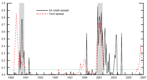
Notes: Probabilities from logit models based on independent variables one year earlier. Shaded areas indicate actual NBER recessions. AA credit spread is based on the ten-year maturity. The term spread is the difference between the 10- and 2-year nominal Treasury yields.

Figure 2. Recession probabilities from univariate models with poor fit

Figure 2 Data

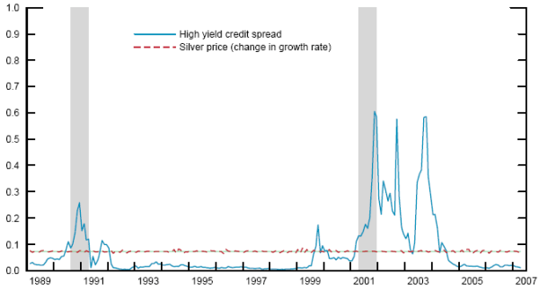
Notes: Probabilities from logit models based on independent variables one year earlier. Shaded areas indicate actual NBER recessions. The high-yield credit spread is based on the ten-year maturity.

Figure 3. Recession probabilities from best bivariate model and model combinations

Figure 3 Data

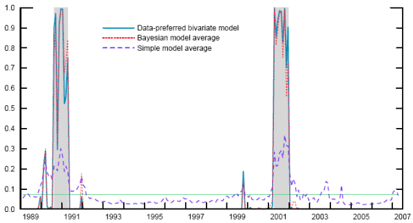
Notes: Probabilities from logit models based on independent variables one year earlier. Shaded areas indicate actual NBER recessions. Bayesian model average is the weighted average of maximum-likelihood estimates, where BIC-approximated marginal likelihoods are used to compute the weights.

Figure 4. Posterior distribution of recession probabilities across parameters and models

Figure 4 Data

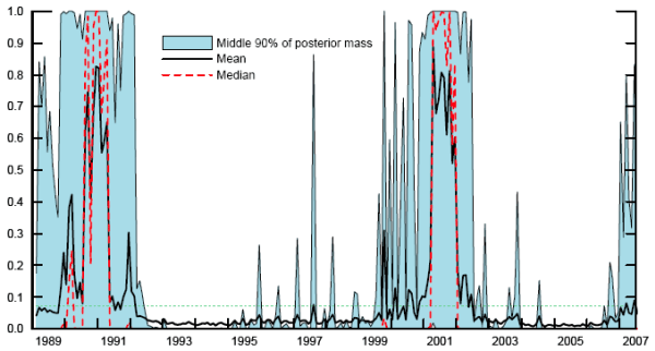
Notes: Probabilities from logit models based on independent variables one year earlier. The figure shows statistics from the full posterior distribution, taking account of both parameter and model uncertainty, as described in Section 5.4.

Footnotes

1. ^* Division of Monetary Affairs, Board of Governors of the Federal Reserve System. Corresponding author: [email protected]; (202)452-2867.

We thank Jonathan Wright and other Federal Reserve Board staff for helpful discussions and Kristen Payne and Ben Johannsen for superb research assistance. The views expressed here are those of the authors and do not represent official positions of the Federal Reserve.

This draft: 14 August 2007 Return to Text

2. See Estrella and Hardouvelis (1991), Estrella and Mishkin (1998), and Estrella, Rodrigues, and Schich (2003). Return to Text

3. See Bernanke (1983), Friedman and Kuttner (1992), Gertler and Lown (2000), and Bordo and Haubrich (2004). Return to Text

4. See Dotsey (1998), Chauvet and Potter (2002, 2005), and Giacomini and Rossi (2006). More recently, Wright (2006) investigated the extent to the predictive performance of a univariate yield-curve model can be improved by including a measure of the current level of interest rates. Return to Text

5. The business press paid close attention to the yield curve's behavior around this time and fretted about its possible implications. (See de Aenlle, C. "Market values: Talk turns to chances of recession." New York Times, 5 Aug. 2006; Hudson, M. "Ahead of the tape." Wall Street Journal, 4 Dec. 2006; and Whitehouse, M. "Bond market cranks up alarm but many investors just shrug." Wall Street Journal, 19 Jan. 2006) However, most economists did not foresee a recession. For example, the Survey of Professional Forecasters registered average predictions of close to 3% for near-term real GDP growth during this time. Return to Text

6. See, among others, McConnell and Perez-Quiros (2000). Notably, the Great Moderation in GDP was not accompanied by a comparable decline in the variability of most asset prices. Return to Text

7. Although the BIC provides a good asymptotic approximation to the marginal likelihood, the relatively small sample that we use, together with the nonlinearity of the logit model, raises the concern that the likelihood may be non-normal. Consequently, the BIC may provide incorrect rankings and weights for the various models. To account for this possibility, we also estimated the marginal likelihoods numerically, for the models ranking highest by BIC. In particular, we ran a Metropolis-Hastings algorithm, using a number of simulations equal to 10,000

$_{m}$ and computed the marginal likelihoods using a modified harmonic-mean estimator (Geweke, 1999). This procedure produced results that were very similar to those given by BIC. Return to Text

8. We note that 1 and 0 probabilities do not necessarily correspond to a "perfect fit." Presumably, the true recession probability was something less than 100% prior to the recession and something greater than 0% prior to the recovery. Since we cannot observe these true probabilities, we cannot precisely measure the model's accuracy, and these exercises must therefore be somewhat informal. Return to Text

9. Our variables are monthly averages of daily values. The implied-volatility measures are constructed from at-the-money options using the Black-Scholes formula. Return to Text

10. We interpolate the quarterly Survey to get monthly expected-inflation values. Return to Text

11. Stock and Watson (1992) and others have noted the failure of the yield curve to match the timing of this recession. Return to Text

^♣ This version is optimized for use by screen readers. Descriptions for all mathematical expressions are provided in LaTex format. A printable pdf version is available. Return to Text