Forecasting Recessions Using Stall Speeds
Keywords: Markov-switching models, business cycles, forecasting
Abstract:
JEL Classification: E32, E37
1 Introduction
This paper examines whether the notion of an economic stall speed has empirical content. By a stall speed, we mean particular values for output growth and other variables, such that when these values are reached during an expansion, the economy has tended to move into a recession within a fairly short time span. Although this notion of a stall speed for output growth has surfaced often in the business press, it appears to have been studied little in academia. The work here fills that void, focusing on two measures of US output, GDP and GDI. Nalewaik (2010a) presents a considerable amount of evidence and logic showing that GDI provides a better measure of output growth than GDP, its better-known counterpart, and in our work here, while stall phases are evident in GDP, they are more plainly visible in GDI.
We study stall speeds in two ways. First, we present non-parametric evidence, examining the distributions of output growth rates immediately before recessions, and these distributions do provide some support for the stall speed notion. Second, we examine Markov switching models that potentially embed stall phases. In particular, we estimate models that include an additional phase of the business cycle, in-between expansions and recessions or in the middle of expansions. While a stall-speed type model may come out of this type of specification, it need not; the parameter estimates may reveal that mid-expansion slow-downs or high-growth recovery phases may be more important features of economy. However, the maximum likelihood parameter estimates show that, for GDI especially, the stall phase is an important feature of the data.
Having established that the stall speed concept is useful in the latest available data, we examine next the usefulness of the Markov-switching models for forecasting recessions in real time. Models using output growth alone appear reasonably useful, producing elevated real time stall probabilities before the onset of some recessions, although the rise in the probabilities is more contemporaneous with the start of other recessions, and the model produces a considerable number of false positive spikes in the stall probabilities.
Finally, we add other important macro variables to the model besides output growth. The change in the unemployment rate is useful for identifying recessions--see also Hamilton (2005)--but less useful for identifying stalls and thus forecasting recessions. We consider two other well-known variables to help identify the stall phases: the slope of the yield curve and the percent change in housing starts. Adding these variables produces models with considerably fewer false positives in real time, and stall probabilities that become elevated well in advance of some recessions; for example, the stall probability from our preferred model was 80 percent in the middle of October 2006, more than a year before the onset of the 2007-9 recession.
The variables added to the model are well-known and should be non-controversial; the contribution of the paper is not in variable selection, but rather in the development of new and innovative ways of employing a fairly standard set of recession-forecasting variables. And the approach taken here, very different from the standard, regression-based forecasting approach, appears promising: GDP-growth forecasts from our preferred Markov-switching model outperform Blue-Chip consensus forecasts at horizons beyond one quarter ahead, and perform particularly well three and four quarters ahead. The model produces these GDP growth forecasts without running a single regression; rather, it relies on the structure of the Markov transition matrix to produce forecasts, and GDP growth is not even in the model when the parameters of that matrix are estimated.
Numerous papers attempt to forecast a binary recession indicator whose dates are determined by the NBER business cycle dating committee, using the slope of the yield curve and other variables in a probit or logit specification.1 The model using the yield curve in this paper can be interpreted as providing a bridge between that literature and the literature using the Markov switching approach of Hamilton (1989, 1990), where the likelihood the economy is in recession is determined not from the NBER dates, but endogenously from the behaviour of real variables in the model such as output growth. The Markov switching models here do that as well, employing real variables that tend to move contemporaneously with the NBER dates. But after the NBER has dated a recession, we incorporate that qualitative information into the model, treating the start and end dates as observed and measured without error as in the binary probit-logit approach.2 Adding the stall phase then allows us to add a recession forecasting aspect to the Markov-switching models as well as a contemporaneous, recession-recognition aspect, naturally leading us to incorporate variables that tend to predict recessions before they actually occur, such as those employed in probit-logit models.
The Markov-switching models in this paper are generally complementary to the probit-logit approach, but there are a few subtle differences. Most importantly, the approach here allows for explicit variability in the length of the stall phase, instead of imposing a fixed lag structure. Using the inversion of the yield curve as a short-hand example, if such an inversion tended to predict the start of a recession on a fairly regular schedule, for example in 12 months as assumed by some models, the probit-logit approach might be appropriate. But that may be asking too much of the data, and it may be that such an inversion can only tell us that a recession is likely at some point in the near future, not precisely when. The yield curve inverted about 7 months before the 2001 recession, but 16 months before the 2007-9 recession, arguing in favor of a model that allows the stall phase to be variable in length.
Section 2 of the paper presents non-parametric evidence for stall speeds in output growth. Section 3 discusses multi-stage Markov switching models, using the latest available data on output growth and related real variables. Section 4 discusses the real time performance of a three-stage Markov switching model using output growth alone, while section 5 adds the other important macroeconomic variables to the model and discusses real time performance. Section 6 concludes.
2 Non-Parametric Analysis
In this section of the paper, we examine output growth time series (as measured by real GDP and real GDI growth) to see if they tend to reach particularly low values in periods soon before the onset of a recession, as defined by the NBER business cycle dating committee, and only rarely in expansion periods not soon followed by a recession. To be more precise, we examine distributions of annualized quarterly output growth rates in the four quarters prior to recessions in the post-war period. Kernel densities for real GDP (top panel) and real GDI (bottom panel) are shown in Figure 1.3 The dashed line shows the kernel density fitting output growth rates in the four quarters prior to recessions, while the solid line show the density fitting output growth rates in other expansion quarters.4 This four-quarter split of the sample is arbitrary, serving only as motivation for the more rigorous models below, which allow for stall phases of variable length, but nonetheless Figure 1 is informative. For either GDP or GDI growth, the density fitting the growth rates preceding recessions peaks at between one and two percent, having considerably more mass to the left of those growth rates than the density fitting the other expansion growth rates, which peaks at close to four percent.
Table 1 cuts the data in a slightly different way, focusing on the left hand side of the distribution of observations. The first two rows of each panel show the cumulative total count of the number of observed growth rates falling below each cutoff considered (0 percent growth, 1 percent, etc), for all expansion quarters and for the four quarters prior to a recession. The third row shows the cumulative distribution for the growth rates four quarters prior to recessions. For example, in the top panel, we see that about a fifth of the real GDI growth rates in the four quarters prior to recessions are below zero and about a third are less than one. The fourth row shows, for observations below each cutoff, the share of the expansion observations that occur in the four quarters prior to recessions. For GDI, the second column shows that sixty four percent (14 out of 22) of expansion observations of below one percent growth were in the four quarters prior to recessions. For GDP, a little less than half (12 out of 25) of expansion observations of below one percent growth were in the four quarters prior to recessions. For both panels, this number drops fairly precipitously as we move to the right in the table, converging towards the fraction of expansion observations occurring in one of the four quarters prior to a recession (which is 43 out of 201 total observations, or about twenty-one percent). Finally, the last row of each panel shows the percentage of recessions where a growth rate in at least one of the preceding four quarters was below the cutoff. For example, eighty two percent of postwar recessions (or 9 out of 11) were preceded by a GDI growth rate of one percent or less in at least one of the four quarters prior to the recession, with the 1953-4 and 1973-5 recessions being the only exceptions the same holds true for GDP, with the 1948-9 and 1953-4 recessions being the only exceptions.
These results suggest that an observed annualized quarterly output growth rate of less than one percent could serve as a moderately useful warning sign that the economy is in danger of falling into recession. Raising the cutoff to two percent (or higher) produces many additional false positive recession signals, or type 2 errors (with the hypothesis being that the economy will soon fall into recession); for real GDI growth, only 2 out of 13 observations between one and two percent occur in the four quarters prior to recessions. And lowering the cutoff to zero percent produces more false negatives or type 1 errors, recessions where the growth rates did not fall below the cutoff in any of the preceding four quarters. It is plainly not possible to possible to identify a stall speed cutoff with no type 1 or type 2 errors, so the usual tradeoff between type 1 and type 2 errors is at play here.
Figure 2 shows the time series of annualized quarterly growth rates of real GDP and real GDI when these growth rates are three percent or less, with a line drawn for the candidate stall speed of one percent. For GDI, several of the false positives occurred in the sluggish recoveries following the 1990-1 and 2001 recessions, suggesting the stall speed cutoff rule may be least useful in such sluggish recoveries, and more useful once an expansion has matured somewhat. For GDP, we see a few more false positives in the middle of expansions, for example in 1967 and 1977. For both measures, some other false positives occurred just before the four quarters preceding a recession: For example, weak GDI growth in 1989Q2 preceded a recession by five quarters, while weak GDP growth in 1956Q1 preceded a recession by six quarters. This emphasizes the need to allow for stall periods of variable length.
Figures 3 and 4 and table 2, follow the format of the first two figures and table using two-quarter annualized changes in the output growth rates. Table 2 shows that, for the two-quarter annualized growth rates, raising the cutoff to around two percent seems appropriate, especially for real GDI growth. More than forty percent of the GDI growth rates in the four quarters prior to recessions were below two, and sixty four percent of growth rates below two (18 out of 28) occurred in the four quarters prior to a recession, with at least one of those growth rates occuring in the four-quarter period preceding eighty-two percent of post-war recessions. Figure 4 shows the only two exceptions were before the 1948-9 and 1953-4 recessions. For real GDP growth, the two percent cutoff works a little less well, echoing the results using the one quarter annualized growth rates. Indeed, the statistics compiled here using the two-quarter annualized growth rates and the two percent cutoff are quite similar to those using the one-quarter growth rates and a one percent cutoff, for both output growth estimates.
Figures 5 and 6 and table 3 examine four-quarter growth rates, smoothing through more of the quarterly volatility in the estimates (in table 3 and figure 5, we drop all quarters from the sample that include any recession quarter in the period over which the four-quarter growth rate is computed). Unfortunately, table 3 shows that, using either output growth measure, these growth rates dip below two percent before only four out of ten recessions in the sample (the 1981-2 recession was dropped from the sample because a four-quarter growth rate before this recession could not be computed due to its proximity to the previous recession), and raising the cutoff to three percent produces many false positive recession signals. So, while the four-quarter growth rates do not appear to be a particularly useful recession forecasting tool, an examination of Figure 6 shows that they might be a useful recession recognition tool: when the two-percent threshold has been breached, the economy has, without fail, either been in recession at some point over the past few quarters, or is about to fall into recession.
While the evidence thus far documents some fairly regular empirical patterns in output growth before recessions, whether these patterns are apparent in real time is a different question, as the estimates for each quarter released by the BEA not long after the quarter ends are revised several times in subsequent years, often changing noticeably around cyclical turning points. However, appendix A shows that the results are not drastically different when we examine the 3rd BEA estimates of GDP and GDI growth available in real time three months after the end of each quarter.
3 Markov Switching Models, Possibly Including Stall Phases
Further evidence that the stall speed notion might be useful comes from the bivariate Markov switching model of Nalewaik (2011), which uses real GDP and real GDI growth to infer probabilities the economy is in either a high-growth state 1 or a low-growth state 2. Earlier work focusing on GDP
growth alone (for example, Hamilton (1989) and subsequent papers) found that the low-growth states from such a model tend to coincide with recessions as defined by the NBER, but Nalewaik (2011) found some subtle differences between the bivariate model-generated low-growth states and recessions. The
maximum likelihood parameter estimates from the model in Nalewaik (2011) are reported in the top panel of table 4, using data available after the BEA released their 3rd 2010Q2 estimates and the 1959Q4 start date employed in the real time analysis below. The first four parameters are the means in
each state, the second three are the parameters of the variance-covariance matrix, assumed the same across states, and the last two parameters are transition probabilities governing the dynamics of the system, telling us the probability the economy will remain in each state in period ![]() if it is in that state in period
if it is in that state in period ![]() . The mean growth rates in the high growth state are each
about four and a half percent, while the mean growth rates in the low-growth state are just slightly under 0 percent for GDP and about minus three-quarters percent for GDI.
. The mean growth rates in the high growth state are each
about four and a half percent, while the mean growth rates in the low-growth state are just slightly under 0 percent for GDP and about minus three-quarters percent for GDI.
These growth rates in low-growth states are higher than the average growth rates of GDP and GDI in recessions, and Figure 7 shows why, plotting the latest smoothed probabilities of the low-growth state for each period in the sample. By smoothed probabilities, we mean two-sided probabilities, where the probability for each period is estimated using the entire sample of output growth rates. We can see that while these probabilities are very high during recessions (shaded gray), they are also elevated for substantial periods of time before some recessions, for example before the 1980 recession, the 1990-1 recession, and the 2007-9 recession. This suggests the Nalewaik (2011) model is combining periods of sluggish growth before recessions, periods we might call the stall phase of an expansion, together with recessions themselves to arrive at its more expansive definition of a low-growth state reflected in its parameters and probabilities. The probabilities of low-growth state are also quite elevated in some periods immediately after the more-recent recessions in the sample (i.e. the 1990-1 and 2001 recessions).
In this paper, we examine models that treat recessions as observed after the NBER business cycle dating committee calls their trough date. Then the maximum likelihood estimates of the mean growth rates of GDP and GDI in the recession state are just the mean growth rates in periods classified as
belonging to that state (see Hamilton and Chauvet, 2005). Similarly, the maximum likelihood estimate of the probability of remaining in the recession state in period ![]() , conditional on being in
the recession state in period
, conditional on being in
the recession state in period ![]() , is simply the number of recession periods followed by another recession period, divided by the total number of recession periods (again, see Hamilton and
Chauvet, 2005). The model partitions expansion quarters into two other possible states, with the recession state classified as state 3. The dynamics of the transition probabilities from state to state are governed by the following transition matrix P:
, is simply the number of recession periods followed by another recession period, divided by the total number of recession periods (again, see Hamilton and
Chauvet, 2005). The model partitions expansion quarters into two other possible states, with the recession state classified as state 3. The dynamics of the transition probabilities from state to state are governed by the following transition matrix P:
| (1) | ![\begin{displaymath}\left( \begin{array}{c} \pi_{t=1} \\ \pi_{t=2} \\ \pi_{t=3} \end{array} \right) = \left[\begin{array}{ccc} p_{11} & p_{21} & 1-p_{33}-p_{32} \\ 1-p_{11} & p_{22} & p_{32} \\ 0 & 1-p_{22}-p_{21} & p_{33} \end{array}\right]\left(\begin{array}{c} \pi_{t-1=1} \\ \pi_{t-1=2} \\ \pi_{t-1=3} \end{array} \right).\end{displaymath}](img3.gif)
|
Initially, we impose only one zero on the matrix: If the economy is in state 1 in any given period, then next period the economy either stays in state 1 (with probability ![]() estimated
by the model) or transitions to state 2 (with probability
estimated
by the model) or transitions to state 2 (with probability ![]() ). The economy cannot pass directly from state 1 into recession, but must pass through an "in-between" state 2 first. We see
little loss of generality in the imposition of this structure, because even if such an "in-between" state does not exist, the model is free to pick a very short duration for state 2, with parameters similar to the recession parameters, and state 2 could then simply cannibalize the first quarter
or two of each recession.5
). The economy cannot pass directly from state 1 into recession, but must pass through an "in-between" state 2 first. We see
little loss of generality in the imposition of this structure, because even if such an "in-between" state does not exist, the model is free to pick a very short duration for state 2, with parameters similar to the recession parameters, and state 2 could then simply cannibalize the first quarter
or two of each recession.5
When the economy is in state 3 (i.e. in a recession), next period the economy either stays in state 3 (with probability ![]() estimated as described earlier), transitions back to the
"in-between" state 2 (which occurs with probability
estimated as described earlier), transitions back to the
"in-between" state 2 (which occurs with probability ![]() ), or transitions to state 1 (with probability
), or transitions to state 1 (with probability
![]() ). If the economy is in the "in-between" state 2, next period the economy either stays in state 2 (with probability
). If the economy is in the "in-between" state 2, next period the economy either stays in state 2 (with probability ![]() ), transitions back to state 1 (with probability
), transitions back to state 1 (with probability ![]() ), or transitions to the recession state 3 (which probability
), or transitions to the recession state 3 (which probability
![]() ). Of course, if
). Of course, if ![]() is high relative to
is high relative to ![]() , a high probability of being in state 2 is not particularly useful for forecasting recessions, and state 2 is often not a "stall phase", but rather something else, perhaps a "pause that
refreshes" in the middle of a maturing expansion. And even if
, a high probability of being in state 2 is not particularly useful for forecasting recessions, and state 2 is often not a "stall phase", but rather something else, perhaps a "pause that
refreshes" in the middle of a maturing expansion. And even if ![]() is low relative to
is low relative to ![]() , the "in-between" state 2 need not correspond to a stall phase. For example, the three state "plucking" model of Friedman (1993) and Sichel (1994) has the exact same structure as the model outlined here. In that model, output growth is rapid in the early stages of an
expansion as the economy moves back towards the trend in potential output and underutilized resources are reemployed, before moderating over the later part of the expansion after output has moved back close to trend; see also Kim and Nelson (1999).
, the "in-between" state 2 need not correspond to a stall phase. For example, the three state "plucking" model of Friedman (1993) and Sichel (1994) has the exact same structure as the model outlined here. In that model, output growth is rapid in the early stages of an
expansion as the economy moves back towards the trend in potential output and underutilized resources are reemployed, before moderating over the later part of the expansion after output has moved back close to trend; see also Kim and Nelson (1999).
Maximum likelihood parameter estimates of this model are reported in the first row of table 5. The model does peg state 1 as the "normal expansion" phase, with mean growth rates in this state very similar to those in the 2-state model in the top panel, while state 2 looks very much like the
"stall" phase of the cycle, with mean GDP growth of one and a half percent and mean GDI growth of about one percent. The mean growth rates in recessions are in the neighborhood of minus one and a half percent. More remarkably, the maximum likelihood estimate of the probability that the economy
moves back into a stall phase after a recession is, to at least four significant digits, zero, as is the maximum likelihood estimate of the probability that the economy moves back to the normal expansion phase after entering the low-growth "in-between" phase 2. This second result shows the stall
speed notion is indeed supported by these data, and is likely to be useful in forecasting recessions, since the economy does not tend to fall into the low-growth state 2 without subsequently falling into recession. State 2 is indeed a stall phase, and the "pause that refreshes", widely discussed
in the mid-1990s, is not an evident feature of these data. With no loss of generality, the last set of parameter estimates in table 5 impose that ![]() and
and ![]() equal zero, so the transition matrix P is:
equal zero, so the transition matrix P is:
| (2) |
|
The smoothed probabilities of state 2 (the solid line) and state 3 (the dotted line) associated with the maximum likelihood parameter estimates in table 5 are shown in Figure 8. The stall phases are indeed of variable length, with fairly long stall phases before the 1990-1 recession and the 2007-9 recessions. Most of the recession probabilities line up fairly well with the NBER dates, although weak growth in 1991 produces fairly high recession probabilities for a few quarters after the end of the 1990-1 recession, and the 2001 recession does not appear clearly in these probabilities.6
To examine these results further, table 6 reports parameter estimates from 3-state Markov-switching models using either GDP alone, GDI alone, or using a related variable. For GDP, when we impose that ![]() and
and ![]() equal zero, the parameter estimates are very close to those in the bivariate model and maintain their stall speed characteristics. These smoothed probabilities
are reported in the top panel of Figure 9. The 2001 recession registers less clearly than in the bivariate model, as we may expect since GDP registered only one quarter of negative growth in that recession. When we do not impose zeros on
equal zero, the parameter estimates are very close to those in the bivariate model and maintain their stall speed characteristics. These smoothed probabilities
are reported in the top panel of Figure 9. The 2001 recession registers less clearly than in the bivariate model, as we may expect since GDP registered only one quarter of negative growth in that recession. When we do not impose zeros on ![]() and
and ![]() , the maximum likelihood estimates shift over to a new equilibrium that looks very different, one where state 1 is a rapid growth
phase and state 2 is a moderate growth phase, somewhat resembling the "plucking" model of Friedman (1993) and Sichel (1994). However, since
, the maximum likelihood estimates shift over to a new equilibrium that looks very different, one where state 1 is a rapid growth
phase and state 2 is a moderate growth phase, somewhat resembling the "plucking" model of Friedman (1993) and Sichel (1994). However, since
![]() , the economy sometimes transitions from the moderate to the rapid growth phase, and since
, the economy sometimes transitions from the moderate to the rapid growth phase, and since
![]() , the economy sometimes transitions from recession directly to the moderate growth phase.
, the economy sometimes transitions from recession directly to the moderate growth phase.
For comparison, the next two rows of table 6 estimate the model using the annualized quarterly growth rates of industrial production (IP), and these estimates look very much like the Friedman-Sichel "plucking" model, whether we impose the zeros on the transition matrix or not.7 When the zeros are not imposed, the estimates assign a positive probability to ![]() , allowing the economy to transition from recession to the moderate growth phase without passing through the rapid growth phase. The smoothed probabilities from this model, plotted along with IP growth in Figure 10, suggest that such a transition occured
following the 1990-1 and 2001 recessions, but the economy transitioned to the rapid growth phase after all other recessions in the sample. Since the maximum likelihood estimate of
, allowing the economy to transition from recession to the moderate growth phase without passing through the rapid growth phase. The smoothed probabilities from this model, plotted along with IP growth in Figure 10, suggest that such a transition occured
following the 1990-1 and 2001 recessions, but the economy transitioned to the rapid growth phase after all other recessions in the sample. Since the maximum likelihood estimate of ![]() is
zero, the economy does not transition back to the rapid growth phase after entering the moderate growth phase; the rapid growth phase occurs exclusively after recessions, as predicted by a plucking-type model.
is
zero, the economy does not transition back to the rapid growth phase after entering the moderate growth phase; the rapid growth phase occurs exclusively after recessions, as predicted by a plucking-type model.
The next two rows of table 6 show that the model using GDI alone prefers a stall-speed model, with the maximum likelihood parameter estimates of ![]() and
and ![]() precisely zero, as in the bivariate model. In the bivariate model, then, it is largely the behavior of GDI that drives the estimates towards a stall-speed model. In general, the bivariate models weight GDI growth
more heavily than GDP growth, because the smaller conditional variance of GDI growth and wider spreads between its means imply that it provides a better signal of the state of the world (see Nalewaik 2011).8 The bottom panel of Figure 9 shows smoothed probabilities from this three-state model. The 2001 recession registers more clearly using GDI than using GDP, not surprising since GDI fell for all three quarters of the recession.
precisely zero, as in the bivariate model. In the bivariate model, then, it is largely the behavior of GDI that drives the estimates towards a stall-speed model. In general, the bivariate models weight GDI growth
more heavily than GDP growth, because the smaller conditional variance of GDI growth and wider spreads between its means imply that it provides a better signal of the state of the world (see Nalewaik 2011).8 The bottom panel of Figure 9 shows smoothed probabilities from this three-state model. The 2001 recession registers more clearly using GDI than using GDP, not surprising since GDI fell for all three quarters of the recession.
Interestingly, the last two rows of table 6 show that a stall-speed model with maximum likelihood parameter estimates of ![]() and
and ![]() equal to zero also obtains using the first difference of the unemployment rate (U). Figure 11 shows smoothed probabilities from this model along with the change in the unemployment rate (defined as the unemployment rate in the last month
of the quarter minus the unemployment rate in the last month of the previous quarter). Clearly, the unemployment rate identifies the 2001 recession more clearly than either output growth measure. The stall periods in figure 11 are somewhat shorter than those for GDI growth, suggesting output growth
enters its stall phase earlier than the change in unemployment, somewhat echoing the end-of-expansion productivity slow-down phenomenon identified by Gordon (1979, 1993, 2003, and 2010).
equal to zero also obtains using the first difference of the unemployment rate (U). Figure 11 shows smoothed probabilities from this model along with the change in the unemployment rate (defined as the unemployment rate in the last month
of the quarter minus the unemployment rate in the last month of the previous quarter). Clearly, the unemployment rate identifies the 2001 recession more clearly than either output growth measure. The stall periods in figure 11 are somewhat shorter than those for GDI growth, suggesting output growth
enters its stall phase earlier than the change in unemployment, somewhat echoing the end-of-expansion productivity slow-down phenomenon identified by Gordon (1979, 1993, 2003, and 2010).
These results suggest that there may be at least four meaningful phases to the business cycle, with the rapid recovery and stall phases appearing with different degrees of clarity in output, industrial production and unemployment. That the high-growth recovery phase is most apparent in IP largely follows from Sichel (1994), who shows that inventory restocking accounts for most of the unusually rapid growth in the early stages of a recovery. Presumably, this inventory restocking is more important for goods, represented by the industrial sector and IP, than for the services, which constitute the bulk of economy-wide measures of output and the labor market.
We did estimate some univariate four-state models, where state 4 is the rapid recovery phase of the plucking model and the transition matrix P is:
| (3) | ![\begin{displaymath}\left( \begin{array}{c} \pi_{t=1} \\ \pi_{t=2} \\ \pi_{t=3} \\ \pi_{t=4} \end{array} \right) = \left[\begin{array}{cccc} p_{11} & p_{21} & p_{31} & 1-p_{44} \\ 1-p_{11} & p_{22} & 0 & 0 \\ 0 & 1-p_{22}-p_{21} & p_{33} & 0 \\ 0 & 0 & 1-p_{33}-p_{31} & p_{44}\end{array}\right]\left(\begin{array}{c} \pi_{t-1=1} \\ \pi_{t-1=2} \\ \pi_{t-1=3} \\ \pi_{t-1=4} \end{array} \right).\end{displaymath}](img16.gif)
|
A positive ![]() implies the economy skips the rapid recovery phase after some recessions. Parameter estimates are reported in table 7 from this model for Real GDI growth and the change
in the unemployment rate, which identified both the stall phase and the rapid recovery phase. The smoothed probabilities from the model fitting the change in the unemployment rate (not shown) suggest the rapid recovery phase occured only after the 1981-2 recession, but the smoothed probabilities
from the model fitting real GDI growth (not shown) show rapid recoveries after each recession up until the mid-1980s. But, predictably, these GDI-based probabilities show a rapid recovery followed neither the 1990-1 recession nor the 2001 recession, and occured with a probability of only around 50
percent for one quarter following the 2007-9 recession.
implies the economy skips the rapid recovery phase after some recessions. Parameter estimates are reported in table 7 from this model for Real GDI growth and the change
in the unemployment rate, which identified both the stall phase and the rapid recovery phase. The smoothed probabilities from the model fitting the change in the unemployment rate (not shown) suggest the rapid recovery phase occured only after the 1981-2 recession, but the smoothed probabilities
from the model fitting real GDI growth (not shown) show rapid recoveries after each recession up until the mid-1980s. But, predictably, these GDI-based probabilities show a rapid recovery followed neither the 1990-1 recession nor the 2001 recession, and occured with a probability of only around 50
percent for one quarter following the 2007-9 recession.
We do not report results from the four-state model using IP growth because it did not identify a meaningful stall phase. This suggests that an important part of some stall phases may have been concentrated in services, a fact that may help explain some of the relative superiority of GDI over GDP in identifying stall phases. Nalewaik (2010a) presents a considerable amount of evidence that, over much of the sample examined here, GDI has been a better measure of economy-wide output than GDP, likely because GDP does a relatively poor job measuring many services industries. If some stall phases have been concentrated in those services industries, that would explain why GDI growth has been better than GDP growth at identifying stalls. For example, the output of real estate and financial services may have been particularly hard hit in the stall phase preceding the 2007-9 recession, and that may have been picked up better by GDI than GDP.
While these results are interesting, differentiating between the early phases of expansions seems extraneous to the main goal of the paper, which is identifying stall phases before NBER-defined recessions. So, in subsequent sections of the paper, we focus on the three-state models including GDI growth, leaving generalizations to four-state models for future research.
4 The Markov Switching Model for Output, Real-Time Estimates
The top panel of Figure 12 shows, using real-time data, the estimated probabilities of the stall state plus the recession state from the bivariate 3-state model, imposing ![]() and
and
![]() equal zero. Specifically, the probability for 1978Q1 is the probability for that quarter computed using the time series from 1959Q4 to 1978Q1 that existed at the end of June 1978 after
the BEA's 3rd release of 1978Q1 data; the 1978Q2 probability uses the time series from the BEA's 3rd release of 1978Q2 data in September 1978; etc. Prior to 1991Q4, we use real GNP and GNI growth instead of real GDP and GDI growth, because those were in fashion at the time. The bottom panel shows
the real-time mean GNI/GDI growth rate estimates.
equal zero. Specifically, the probability for 1978Q1 is the probability for that quarter computed using the time series from 1959Q4 to 1978Q1 that existed at the end of June 1978 after
the BEA's 3rd release of 1978Q1 data; the 1978Q2 probability uses the time series from the BEA's 3rd release of 1978Q2 data in September 1978; etc. Prior to 1991Q4, we use real GNP and GNI growth instead of real GDP and GDI growth, because those were in fashion at the time. The bottom panel shows
the real-time mean GNI/GDI growth rate estimates.
Note that, in this analysis, we treat a recession as observed for purposes of computing recession parameters only after the NBER has declared both its peak and its trough, to be extra conservative and make sure we do not employ any information that would not have been known in real time. For example, since the NBER declared the troughs of the 1981-2 and 1990-1 recessions on July 8, 1983 and on December 22, 1992, respectively, for releases between those two dates, we treat only recessions up to and including the 1981-2 recession as observed. Similarly, between December 22, 1992 and July 17, 2003 (the announcement date of the 2001 recession trough), we treat recessions up to and including the 1990-1 recession as observed; between July 17, 2003 and September 20, 2010 (the announcement date of the 2007-9 recession trough), we treat recessions up to and including the 2001 recession as observed, and for the last release in our sample, the only one after September 20, 2010, we treat the 2007-9 recession as observed.
The real-time estimates in Figure 12 show some modest successes and some notable failures. Among the successes, the probability of recession plus stall jumped up to around 90 percent after the 3rd BEA release of 1979Q2 data in September 1979, several months before the start of the 1980 recession, and the probability jumped up above 60 percent after the 3rd BEA release of 2007Q1 data in June 2007, six months before the start of the 2007-9 recession, although it ticked back down to around 40 percent three months later before jumping back up to around 90 percent in December 2007. For the 1990-1 and 2001 recessions, the rise in the probabilities was more contemporaneous with the start of the recession, or slightly lagging, given the reporting delays. Overall, this stall speed model provides a somewhat early warning sign before some recessions, but not all of them.
Counterbalancing these modest successes are some false positive stall signals, some related to model- and parameter-instability. The dotted line in the bottom panel of Figure 12 shows that the mean growth rate in the stall state stays between 0.5 and 2 percent, except for a brief period in the mid-1990s, when it jumps up to almost 3 percent. These estimates followed the 1995 benchmark revision to the NIPA accounts, which revised the entire historical time series, and these particular revisions led the model to switch over to something more like the "plucking" model, with smoothed probabilities of state 2 elevated for the better part of several expansions. So while these high probabilities are a "false positive" in some sense, it is not because the model thought the economy was entering a stall phase. Rather, the model thought the economy was entering its "normal expansion" phase after passing through its "rapid recovery" phase. Interestingly, over this whole series of estimates, this is the only time the bivariate model switches over to something like a plucking model, and it soon switches back to the stall speed model.
During the extended set of elevated probabilities in the mid-1980s, the mean in state 2 was relatively high, but the model still looks like a stall speed model, so this is more of a pure set of extended false positive readings. In 1991, the probabilities are slow to come down after the end of the recession, due to sluggish growth. And in 2003, elevated readings occur primarily because of weakness in real GDI growth at that time, coupled with the shallowness of the 2001 recession, which causes the model to misclassify the period from late 2000 to early 2003 as an extended stall phase.
Figure 13 compares the real-time probabilities of the low-growth state from the bivariate two-state Markov switching model in Nalewaik (2011), the solid line, with the real-time probabilities of the stall state plus the recession state from the bivariate three-state model, the dotted line. While the false positives in the mid-1980s and mid-1990s do not occur in the two-state model, a marked advantage to that model, we also see some advantages to the three-state model. First, the probability of either stall or recession stays more consistently elevated before the recessions starting in 1980 and 2007. Second, and more subtly, the recession probability comes down slightly faster after the end of some recessions. This occurs because the spread between the means in the expansion and recession states in the three-state model is wider than the spread between the means in the high- and low-growth states in the two-state model, allowing the three-state model to signal the transition from recession to expansion more quickly. Again, for more details on how this logic works, see Nalewaik (2011).
While the analysis so far uses the time series that were actually available in real time, we made no distinction between the observations at the end of the sample that have been little revised (i.e. the 3rd current quarterly estimates), and those that have passed through annual and benchmark revisions. Appendix A provides some analysis of the statistical properties of the 3rd current quarterly estimates, and shows how they differ from the revised estimates.
5 Markov Switching Models, Augmented with Additional Variables
Adding an explicit stall phase to the Markov switching model raises the question of whether we could better identify the stall phase by incorporating information from other variables. Directly adding additional variables to the model is the easiest way to proceed, but things did not work out so well when we added our first new variable, the slope of the yield curve (TERM), measured as the difference in yields between 10-year Treasury bonds and 3-month Treasury bills. Essentially, the model is able to partition states 1 and 2 in a way that fits TERM so well that it focuses on fitting TERM alone in expansions, ignoring the behavior of output growth so that state 2 loses its stall phase characteristics. Figure 14 shows TERM and smoothed probabilities from a model that substitutes TERM for GDP growth, where we see probabilities of state 2 staying high for long time periods in the 1960s and the second half of the 1990s, when the slope of the yield curve was relatively flat. A stall phase that lasts five years is not meaningful for our purposes, so adding TERM to the model in this way is not a viable option.
Adding the change in the unemployment rate (U) and the log change in the quarterly average of housing starts (STARTS) poses no such problems. We weight the log change in housing starts by the nominal share of residential investment in GDP, so that it represents (approximately) a contribution to GDP growth. Output growth and the unemployment rate are economy-wide aggregates, but residential investment is a small component of the economy whose share of output fluctuates wildly over the business cycle, so weighting in this way makes sense as a way to crudely capture the changing importance of this component for the overall economy. For example, in the summer and fall of 2010, when many analysts were concerned that the economy might be entering a double-dip recession, one argument against that outlook was that the output share of cyclically-sensitive sectors was already extremely low, around 2 percent of nominal GDP in the case of housing, implying that a renewed downturn in those sectors was less likely to drag down the economy as a whole than in say, early 2006, when that housing share was at an extremely-elevated 6 percent.
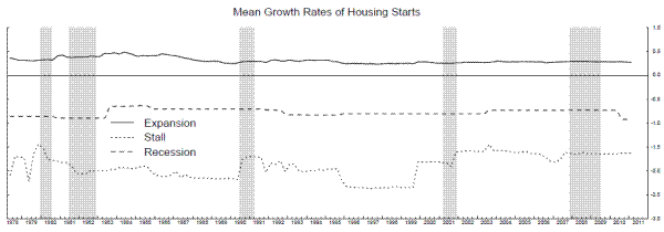
GDP arguably adds little to the model when GDI is available, so we examine a three-variable model with the STARTS contribution, GDI, and U. Parameters estimated from 1964Q2 to 2010Q2 are reported in the first two panels of table 8A. The change in U is generally useful in identifying recessions. The difference between its mean in the recession state, where it rises six tenths of a percentage point per quarter, and the mean in the stall state, where it rises less than one tenth of a percentage point per quarter, is 2.3 times its conditional standard deviation. For GDI growth, the difference between the stall and recession means is only 1.1 times its standard deviation, so the recession signals it provides are less sharp. STARTS is not useful for identifying the transition from the stall phase to recession, since it actually subtracts less from GDP growth in recessions than in stalls. For identifying stalls, the difference between the mean in the expansion state and the mean in the stall state is the relevant number, a difference that amounts to 0.8 standard deviations for U and about 1.4 standard deviations for both GDI and STARTS. So, both GDI and STARTS are moderately useful for identifying stalls. Smoothed probabilities from this model, along with STARTS, are plotted in Figure 15. The stall phases and recession probabilities look reasonable.
To get the information from TERM into the model, we use the techniques in Nalewaik (2010b) for incorporating forecasts into Markov switching models. The conditional means and variance of TERM are estimated in a second stage using the smoothed probabilities from the first stage model estimated in table 8A; these are the first three parameters in Table 8B. The means of TERM in the normal expansion state 1 and in the recession state 3 are both about 1.7 percent, but in the stall state 2 (where the stall state is determined by STARTS, GDI, and U, not by TERM itself), TERM averages only 0.1 percent. The first element of the variance-covariance matrix below shows the difference between the mean in the normal expansion state and the stall state is about 1.5 standard deviations, so TERM does appear likely to be useful for identifying stalls. Table 8B reports parameter estimates for four lags of TERM as well as its contemporaneous value, showing that the third and fourth lags of TERM are useful for differentiating between expansions and recessions. For example, a value for TERM four quarters ago of around a 0.3 percent suggests the economy is still in recession, while a value for TERM four quarters ago of 1.8 percent suggests the economy is back in a normal expansion phase.
TERM is more timely than the BEA estimates, so one way to incorporate the information in TERM is to roll the probabilities forward one quarter and update them using the conditional distributions of TERM and its lags, as in Nalewaik (2010b).9 For example, the 3rd BEA estimates for 2010Q2 were released in late September 2010, but by close of business on the last day of September, a few days later, the 2010Q3 value of TERM was known, allowing us to update probabilities for that next quarter using the information in TERM. Usually less than a week after we observe that value for TERM, we observe U for the next quarter (available the first Friday of first month of the quarter), and a couple of weeks after that, we observe the value for STARTS for the next quarter (released around the middle of the first month of the quarter), allowing us to update the probabilities with the information from these variables as well.
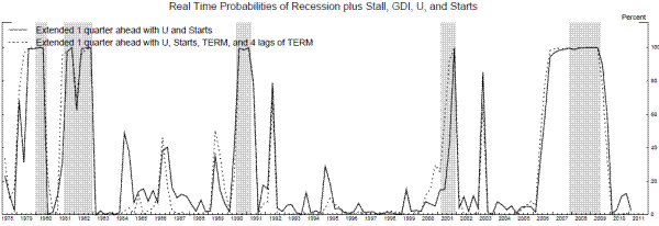
Figure 16 shows probabilities estimated for the latest quarter in real time, where the latest quarter has been partially updated as described above. So the timing here is somewhat different than in Figures 12 and 13; for example, the 1978Q1 estimates plotted in Figure 16 were available after the March 1978 STARTS data was released in the middle of April 1978. The dotted line shows probabilities for the latest quarter updated using U, STARTS, TERM and its four lags, while the solid line shows these probabilities updated using U and STARTS only.10 Note that although GDI is not employed to update the probability for the latest quarter, it remains very influential because the probability for the latest quarter is strongly influenced by the probability from the previous quarter through the Markov transition matrix P, and that previous-quarter probability reflects the information from GDI. Although the unemployment rate and housing starts revise little, we compute these probabilities using real time data from various BEA databases and publications and from the Philadelphia Fed's real time dataset.
Compared to Figure 12, the most striking feature of Figure 16 is the lack of false positives. We see only two individual quarters of false positive spikes higher than 50 percent in the stall probabilities, one in the midst of the jobless recovery after the 1990-1 recession and the other in the jobless recovery after the 2001 recession. Furthermore, these probabilities provide considerable advance warning ahead of some recessions, especially when the probabilities are updated using TERM as well as U and STARTS. For example, in the middle of April 1979, nine months before the onset of the 1980 recession, the model shows the probability that the economy entered a stall phase in 1979Q1 was about 75 percent, rising to 96 percent three months later. After that initial rise, the probabilities of either stall or recession remain close to 100 percent until the middle of October 1980, when they show a high likelihood the economy moved back into an expansion phase in 1980Q3, which turned out to be correct. The expansion probabilities remain high until the middle of July 1981, the month the 1981-2 recession officially started, when the probabilities updated with TERM show a 96 percent probability the economy entered a stall phase in 1981Q2. The probabilities of stall or recession remain elevated until April 1983, when they show a 100 percent probability the economy moved back into an expansion phase in 1983Q1, which again turned out to be accurate.
In July 1989, the model updated using TERM shows a 51 percent probability the economy entered a stall phase in 1989Q2, but this stall probability came back down to 3 percent by April 1990, so the real time identification of the stall phase was not so good before the 1990-1 recession. The timing of the spike back up in the recession probability in 1990 was determined by the data available in real time on GNI. In particular, the spike occured with the annual revision accompanying the BEA's 1990Q2 "advance" data release in late July 1990, coinciding with the official recession start date. These revisions showed that GNI growth in 1989 was much weaker than initially thought, and clarified the fact that the economy was indeed in a stall phase in 1989; see Nalewaik (2011) for more details.
Of the five recessions analyzed here, the 2001 recession was picked up least well by the probabilities updated using U and STARTS, which showed relatively little weakness ahead of and early in that downturn. However, TERM did turn down ahead of that recession, providing some advance warning. In the mid-January 2001, the model using TERM showed a 30 percent probability that the economy entered a stall phase in 2000Q4, and in mid-July 2001, model showed a 58 percent probability that the economy was in either a stall or recession in 2010Q2, the first quarter of the 2001 downturn. In April 2002, both probabilities show the economy likely moved back to expansion in 2002Q1, which turned out to be accurate.
The probabilities from this model provided the longest advance warning ahead of the 2007-9 downturn. In the middle of October 2006, the model updated using TERM showed an 80 percent probability that the economy entered a stall phase in 2006Q3. The corresponding probability updated using U and STARTS alone was also very elevated at 59 percent, a probability with rose to 94 percent three months later. After that, the probabilities of stall plus recession remain very high until January 2010, when the probabilities updated with TERM show a 66 percent chance the economy entered an expansion phase in 2009Q4, one quarter after the NBER trough.
Table 8C evaluates the real time forecasting performance of the Markov switching model updated with TERM by comparing its point forecasts with Blue Chip consensus forecasts. Forecasts ![]() quarters ahead from the Markov switching model are easily constructed by taking the real time probabilities for each quarter, and iterating those forward using the transition matrix
quarters ahead from the Markov switching model are easily constructed by taking the real time probabilities for each quarter, and iterating those forward using the transition matrix ![]() to
produce the probabilities governing the expected state of the world
to
produce the probabilities governing the expected state of the world ![]() periods ahead. Forecasts are then computed by multiplying these probabilities by the conditional means of the variable of
interest. Conditional means for any variable, even one not included in the model, can be computed easily as weighted averages using the smoothed probabilities as weights. In this comparison we focus on GDP growth, examining forecasts from zero quarters ahead (where the zero-quarter-ahead forecast
for any quarter is produced in the first month of that quarter, for both Blue Chip and the model) to ten quarters ahead, although the Blue Chip forecasts are available on a consistent basis only out to four quarters ahead.
periods ahead. Forecasts are then computed by multiplying these probabilities by the conditional means of the variable of
interest. Conditional means for any variable, even one not included in the model, can be computed easily as weighted averages using the smoothed probabilities as weights. In this comparison we focus on GDP growth, examining forecasts from zero quarters ahead (where the zero-quarter-ahead forecast
for any quarter is produced in the first month of that quarter, for both Blue Chip and the model) to ten quarters ahead, although the Blue Chip forecasts are available on a consistent basis only out to four quarters ahead.
The top panel of the table shows that, from 1981Q3 to 2010Q3, the Blue Chip forecasts zero quarters ahead have smaller root-mean-square forecast errors (RMSFE) than the forecasts from the Markov switching model. This was expected, since there is no substitute for closely tracking the incoming spending data when forecasting GDP growth in the near term, and the Markov switching model does not do that. But the Markov-switching model produces comparable-sized forecast errors one quarter ahead, and as the forecast horizon increases, the magnitude of the RMSFE increases more rapidly for the Blue Chip forecasts than for the Markov-switching forecasts. The unconditional standard deviation of GDP growth was 2.87 percentage points over this sample, so the Blue Chip consensus exhibits essentially zero (actually, slightly negative) forecasting ability beyond two quarters ahead.
The next two panels reports results from splitting the out-of-sample period. One panel shows RMSFE in periods classified as either recessions or stalls, where stalls are crudely defined as in section 2 (i.e. as the four quarters immediately preceding a recession), while the other panel shows RMSFE in all other expansion periods. As expected, the relative accuracy of the Markov-switching forecasts at longer horizons is concentrated in recessions and stall periods.11 Finally, the bottom panel shows that the superiority of the Markov-switching forecasts is particularly pronounced over the last two business cycles, from 1993Q2 to 2010Q3. This is partly the case because, over this more-recent sample, the long-horizon Markov-switching forecasts are more accurate in normal expansion periods as well as in stall and recession periods. At the three- and four-quarter ahead forecast horizons, the RMSFE from the Markov-switching model are 12 to 14 percent smaller than those from the Blue Chip consensus; the bolding shows that the differences between the squared forecast errors at these horizons are statistically significant at the 5 percent significance level, using Diebold-Mariano standard errors with eight lags. The unconditional standard deviation of GDP growth was 2.62 percentage points over the 1993Q2 to 2010Q3 sample, so while Blue Chip again exhibits no forecasting ability beyond one-quarter ahead, the Markov-switching model does.
It is notable that this long-horizon forecasting ability seems to stem primarily from the structure of the Markov-switching model, not from the selection of variables included in the model. So, while the slope of the yield curve and the change in housing starts are good long-horizon forecasting
variables, using these two variables to forecast GDP growth recursively using OLS regressions yields three- and four-quarter ahead forecasts with RMSFE 13 to 14 percent larger than those from the switching model. Such regression-based approaches are standard, and, indeed, ubiquitous in economic
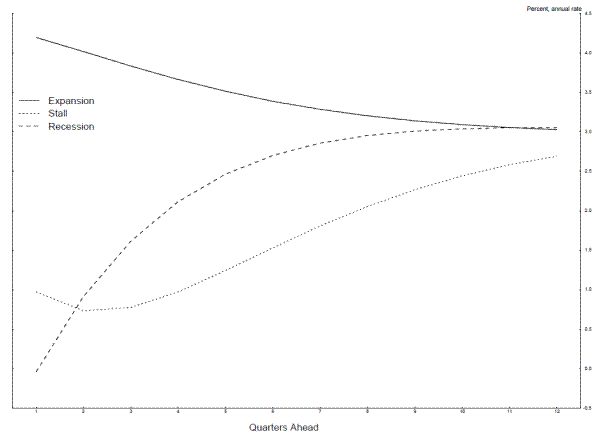
forecasting, so it is interesting that the Markov-switching model does better by taking an entirely different approach to forecasting. The Markov-switching model does not estimate a single regression to construct its forecasts, but rather relies on the transition matrix ![]() to construct forecasts extending arbitrarily far ahead. Figure 17 gives more insight into how this works, and why the Markov-switching model might be particularly good at forecasting beyond one quarter
ahead. Conditional on 100 percent probability of being in a particular state of the world in period 0, the figure shows GDP growth forecasts from
to construct forecasts extending arbitrarily far ahead. Figure 17 gives more insight into how this works, and why the Markov-switching model might be particularly good at forecasting beyond one quarter
ahead. Conditional on 100 percent probability of being in a particular state of the world in period 0, the figure shows GDP growth forecasts from ![]() to 12 quarters ahead, again just the probabilities computed using the iterated transition matrix
to 12 quarters ahead, again just the probabilities computed using the iterated transition matrix ![]() multiplied by the
three conditional means, which are 4.4 percent in state one, 1.7 percent in state two, and -1.3 percent in state three.
multiplied by the
three conditional means, which are 4.4 percent in state one, 1.7 percent in state two, and -1.3 percent in state three.
Conditional on starting out in either the expansion state (see the solid line) or the recession state (see the dashed line), the forecasts converge monotonically and fairly rapidly to the long-run steady-state growth rate of around 3 percent. However, conditional on starting out in the stall state (see the dotted line), the forecasts initially move down away from the steady-state, as the probability the economy transitions from the stall state to recession increases. The predicted values bottom out at around 0.7 to 0.8 percent at the two- and three-quarters ahead horizon, and remain below 1 percent four quarters ahead before rising to about 2 percent eight quarters ahead. Essentially, a successful determination that the economy is in the stall state allows a forecaster to project GDP growth that is well below average far into the future, since the economy is likely to stay in the stall state for a time before falling into the recession state. This fact seems to account for much of the relative forecasting success of this model at horizons beyond a quarter or so ahead.
The forecast conditional on starting out in the stall state in Figure 17 is obviously not modal, and may look highly implausible under the structure of the model. Specifically, an analyst familiar with the stall speed notion may object to such a forecast, arguing that the economy could not
experience such slow growth for so long without falling into recession. This logic is absolutely correct if the goal is to produce a modal forecast; the modal forecast here would be 1.7 percent in periods one to three, periods where the modal probability puts the economy in the stall state, -1.3
percent in periods four to six, periods where the modal probability puts the economy in recession, and 4.4 percent in period seven and beyond, periods where the modal probability puts the economy in expansion. But similar to the case of forecasting a binary variable which takes on a value of 1 with
probability ![]() and 0 otherwise, where the optimal forecast (in the sense of minimizing RMSFE) is not 1 but rather
and 0 otherwise, where the optimal forecast (in the sense of minimizing RMSFE) is not 1 but rather ![]() , the optimal forecast here is not the modal forecast, but rather one that probabilistically averages over many different possible paths for the economy, each with a different set of lengths for the stall phase and the recession phase.
, the optimal forecast here is not the modal forecast, but rather one that probabilistically averages over many different possible paths for the economy, each with a different set of lengths for the stall phase and the recession phase.
6 Concluding Remarks
We have presented both non-parametric evidence and parametric evidence from Markov switching models showing that the economic stall speed concept has some empirical content, and can be moderately useful in forecasting recessions. While real time analysis of the Markov switching models using output growth (i.e. GDP and GDI growth) alone shows they have exhibited a fair number of false positive recession signals, adding some additional variables to the model considerably reduces the incidence of false positives. Specifically, the slope of the yield curve and the percent change in housing starts are useful for identifying the stall phase of the cycle, while the change in the unemployment rate is useful for identifying recessions themselves. Interestingly, the false positive recession signals that remain are in the sluggish, jobless recoveries immediately following the 1990-1 and 2001 recessions, suggesting an important caveat to our results. The dynamics at play in the early part of the 1990s and 2000s expansions may have been different than the dynamics at play in the more-mature part of those and other expansions, and our stall speed models may have omitted an additional phase of the business cycle that has appeared in recent decades, namely the sluggish, jobless recovery phase.12 If so, the applicability of these stall speed models may be somewhat limited at certain times, such as in the middle of 2010 when the economy evidently slowed while still in the early stages of recovery from the 2007-9 recession.
Going forward, the accuracy of these stall speed models will depend on the success of the Federal Reserve and other policymakers in anticipating economic weakness and heading it off with timely policy actions. Recessions have become less frequent since the mid-1980s, which may be related to policy: the elevated stall probabilities in the mid-1980s, mid-1990s, and possibly even in early 2003, may have been cases where the economy was in the early stages of a stall, but monetary easing averted an imminent recession. If the Fed anticipates and averts more recessions going forward, the stall-speed models may not work as well, in the sense that they may show more false positive stall readings. However, if the Fed does become better at preventing the types of recessions we have seen in the past, future recessions may start in ways that are difficult to anticipate based on current data and knowledge. In that case, the stall-speed models again may not work as well going forward, but the economy would not necessarily experience fewer recessions.
The results in the paper open up other questions. It may be that the stall phase of the business cycle has little economic content, and occurs simply because the economy moves somewhat slowly, so an "in-between" phase must exist between recessions and expansions.13 But a slow-moving economy seems unlikely to be the whole story, and the stall phase may be driven by interesting economic mechanisms. Linking the empirical results here to economic models that embed such mechanisms, producing non-linear, "knife-edge" dynamics, may be an interesting avenue for future research.
Tables and Figures
Table 1A: Real GDI, quarterly annualized percent change, 1947Q2-2007Q4:
| Cutoff | 0 | 1 | 2 | 3 |
| Cumulative Frequency < cutoff (Total) | 13 | 22 | 35 | 69 |
| Cumulative Frequency < Cutoff (4 qtrs before recession) | 9 | 14 | 16 | 26 |
| Cumulative Distribution (4 qtrs before recession) | 21% | 33% | 37% | 60% |
| Percent obs < cutoff occuring in 4 qtrs before recession | 69% | 64% | 46% | 38% |
| Percent of Recessions with any of 4 qtrs prior < cutoff | 64% | 82% | 91% | 100% |
Table 1B: Real GDP, quarterly annualized percent change, 1947Q2-2007Q4:
| Cutoff | 0 | 1 | 2 | 3 |
| Cumulative Frequency < cutoff (Total) | 11 | 25 | 43 | 72 |
| Cumulative Frequency < Cutoff (4 qtrs before recession) | 7 | 12 | 16 | 24 |
| Cumulative Distribution (4 qtrs before recession) | 16% | 28% | 37% | 56% |
| Percent obs < cutoff occuring in 4 qtrs before recession | 64% | 48% | 37% | 33% |
| Percent of Recessions with any of 4 qtrs prior < cutoff | 55% | 82% | 82% | 100% |
Table 2A: Real GDI, 2-quarter annualized percent change, 1947Q3-2007Q4:
| Cutoff | 0 | 1 | 2 | 3 |
| Cumulative Frequency < cutoff (Total) | 5 | 14 | 28 | 52 |
| Cumulative Frequency < Cutoff (4 qtrs before recession) | 4 | 9 | 18 | 22 |
| Cumulative Distribution (4 qtrs before recession) | 10% | 21% | 43% | 52% |
| Percent obs < cutoff occuring in 4 qtrs before recession | 80% | 64% | 64% | 42% |
| Percent of Recessions with any of 4 qtrs prior < cutoff | 27% | 45% | 82% | 100% |
Table 2B: Real GDP, 2-quarter annualized percent change, 1947Q3-2007Q4:
| Cutoff | 0 | 1 | 2 | 3 |
| Cumulative Frequency < cutoff (Total) | 1 | 12 | 25 | 62 |
| Cumulative Frequency < Cutoff (4 qtrs before recession) | 0 | 5 | 12 | 21 |
| Cumulative Distribution (4 qtrs before recession) | 0% | 12% | 29% | 50% |
| Percent obs < cutoff occuring in 4 qtrs before recession | 0% | 42% | 48% | 34% |
| Percent of Recessions with any of 4 qtrs prior < cutoff | 0% | 45% | 73% | 100% |
Table 3A: Real GDI, 4-quarter percent change, 1948Q1-2007Q4:
| Cutoff | 0 | 1 | 2 | 3 |
| Cumulative Frequency < cutoff (Total) | 2 | 5 | 13 | 38 |
| Cumulative Frequency < Cutoff (4 qtrs before recession) | 2 | 5 | 11 | 19 |
| Cumulative Distribution (4 qtrs before recession) | 5% | 13% | 28% | 49% |
| Percent obs < cutoff occuring in 4 qtrs before recession | 100% | 100% | 85% | 50% |
| Percent of Recessions with any of 4 qtrs prior < cutoff | 10% | 20% | 40% | 80% |
Table 3B: Real GDP, 4-quarter percent change, 1948Q1-2007Q4:
| Cutoff | 0 | 1 | 2 | 3 |
| Cumulative Frequency < cutoff (Total) | 0 | 1 | 10 | 43 |
| Cumulative Frequency < Cutoff (4 qtrs before recession) | 0 | 1 | 7 | 20 |
| Cumulative Distribution (4 qtrs before recession) | 0% | 3% | 18% | 51% |
| Percent obs < cutoff occuring in 4 qtrs before recession | 0% | 100% | 70% | 47% |
| Percent of Recessions with any of 4 qtrs prior < cutoff | 0% | 10% | 40% | 80% |
|
|
|
|
|
|
|
|
||
| 4.42 | 4.60 | -0.16 | -0.71 | 8.66 | 6.29 | 5.61 | 0.93 | 0.82 |
|---|---|---|---|---|---|---|---|---|
| (0.27) | (0.24) | (0.51) | (0.51) | (0.90) | (0.70) | (0.70) | (0.02) | (0.06) |
|
|
|
|
|
|
|
|
|
|
|||||
| 4.55 | 4.72 | 1.50 | 0.96 | -1.28 | -1.51 | 8.06 | 6.04 | 5.18 | 0.94 | 0.75 | 0.77 | 0.00 | 0.00 |
|---|---|---|---|---|---|---|---|---|---|---|---|---|---|
| (0.26) | (0.24) | (0.68) | (0.64) | (0.83) | (0.65) | (0.88) | (0.66) | (0.67) | (0.02) | (0.13) | (0.11) | (0.04) | (0.07) |
| 4.55 | 4.72 | 1.50 | 0.96 | -1.28 | -1.51 | 8.06 | 6.04 | 5.18 | 0.94 | 0.75 | 0.77 | ||
| (0.26) | (0.24) | (0.69) | (0.67) | (0.85) | (0.73) | (0.90) | (0.68) | (0.70) | (0.02) | (0.10) | (0.09) |
| Variable |
|
|||||||||
| GDP | 4.50 | 1.55 | -1.28 | 8.11 | 0.94 | 0.74 | 0.77 | -531.91 | ||
| GDP | (0.36) | (1.03) | (1.03) | (1.01) | (0.02) | (0.19) | (0.09) | |||
| GDP | 7.48 | 3.20 | -1.28 | 6.28 | 0.64 | 0.90 | 0.77 | 0.04 | 0.07 | -529.83 |
| GDP | (0.72) | (0.34) | (0.77) | (0.91) | (0.11) | (0.04) | (0.09) | (0.04) | (0.08) | |
| IP | 8.49 | 3.07 | -6.42 | 17.98 | 0.86 | 0.90 | 0.77 | -630.65 | ||
| IP | (0.67) | (0.47) | (0.97) | (2.01) | (0.05) | (0.04) | (0.08) | |||
| IP | 8.70 | 3.11 | -6.42 | 17.82 | 0.87 | 0.94 | 0.77 | 0.00 | 0.03 | -629.58 |
| IP | - | - | (0.86) | - | - | - | (0.08) | - | (0.04) | |
| GDI | 4.71 | 1.02 | -1.51 | 6.03 | 0.94 | 0.73 | 0.77 | -508.93 | ||
| GDI | (0.24) | (0.84) | (0.73) | (0.67) | (0.02) | (0.12) | (0.09) | |||
| GDI | 4.71 | 1.02 | -1.51 | 6.03 | 0.94 | 0.73 | 0.77 | 0.00 | 0.00 | -508.93 |
| GDI | (0.24) | (0.82) | (0.69) | (0.64) | (0.02) | (0.18) | (0.11) | (0.07) | (0.06) | |
| U | -0.12 | 0.11 | 0.58 | 0.06 | 0.94 | 0.65 | 0.77 | -37.20 | ||
| U | (0.02) | (0.07) | (0.07) | (0.01) | (0.02) | (0.15) | (0.08) | |||
| U | -0.12 | 0.11 | 0.58 | 0.06 | 0.94 | 0.65 | 0.77 | 0.00 | 0.00 | -37.20 |
| U | (0.01) | (0.05) | (0.07) | (0.01) | - | (0.16) | (0.07) | - | - |
| Variable | |||||||||||
| GDI | 3.98 | 0.27 | -1.51 | 5.90 | 5.57 | 0.92 | 0.69 | 0.77 | 0.88 | 0.00 | 0.07 |
| GDI | (0.37) | (1.00) | - | (0.45) | (0.59) | (0.02) | (0.05) | (0.09) | (0.06) | - | (0.05) |
| U | -0.10 | 0.11 | 0.58 | -0.59 | 0.05 | 0.94 | 0.62 | 0.77 | 0.82 | 0.00 | 0.20 |
| U | (0.02) | (0.07) | (0.06) | (0.10) | (0.01) | (0.03) | (0.19) | (0.08) | (0.16) | (0.23) | (0.07) |
|
|
|
|
|
|
|
||||||
| 0.28 | -1.62 | -0.92 | 4.53 | 1.20 | -1.62 | -0.12 | 0.06 | 0.60 | 0.94 | 0.77 | 0.77 |
|---|---|---|---|---|---|---|---|---|---|---|---|
| (0.12) | (0.29) | (0.34) | (0.23) | (0.50) | (0.56) | (0.02) | (0.05) | (0.06) | (0.02) | (0.08) | (0.08) |
| 1.85 | ||
|---|---|---|
| 0.53 | 6.09 | |
| -0.08 | -0.28 | 0.05 |
|
|
|
|
|
|
|
|
|
|
|
|
|
|||
| 1.74 | 0.12 | 1.66 | 1.85 | 0.08 | 1.13 | 1.89 | 0.20 | 0.69 | 1.87 | 0.44 | 0.39 | 1.83 | 0.73 | 0.31 |
|---|---|---|---|---|---|---|---|---|---|---|---|---|---|---|
| (0.10) | (0.21) | (0.23) | (0.10) | (0.20) | (0.26) | (0.10) | (0.20) | (0.28) | (0.10) | (0.21) | (0.30) | (0.10) | (0.21) | (0.31) |
| TERMt | TERMt-1 | TERMt-2 | TERMt-3 | TERMt-4 |
|---|---|---|---|---|
| 1.20 | ||||
| 0.92 | 1.17 | |||
| 0.77 | 0.89 | 1.16 | ||
| 0.72 | 0.73 | 0.89 | 1.18 | |
| 0.56 | 0.69 | 0.73 | 0.91 | 1.21 |
| Quarters Ahead: | 0 | 1 | 2 | 3 | 4 | 5 | 6 | 7 | 8 | 9 | 10 |
| RMSFE, 1981Q3-2010Q3: Markov-Switching | 2.43 | 2.59 | 2.73 | 2.82 | 2.79 | 2.82 | 2.83 | 2.82 | 2.84 | 2.86 | 2.88 |
| RMSFE, 1981Q3-2010Q3: Blue-Chip Consensus | 2.30 | 2.65 | 2.86 | 2.94 | 2.95 | ||||||
| RMSFE, 1981Q3-2010Q3, stalls and recessions: Markov-Switching | 3.11 | 3.61 | 4.04 | 4.27 | 4.16 | 4.20 | 4.19 | 4.19 | 4.26 | 4.31 | 4.37 |
| RMSFE, 1981Q3-2010Q3, stalls and recessions: Blue-Chip Consensus | 2.95 | 3.87 | 4.39 | 4.57 | 4.56 | ||||||
| RMSFE, 1981Q3-2010Q3, normal expansions: Markov-Switching | 2.14 | 2.14 | 2.12 | 2.14 | 2.17 | 2.19 | 2.21 | 2.20 | 2.17 | 2.18 | 2.17 |
| RMSFE, 1981Q3-2010Q3, normal expansions: Blue-Chip Consensus | 2.06 | 2.09 | 2.11 | 2.14 | 2.17 | ||||||
| RMSFE, 1993Q2-2010Q3: Markov-Switching | 2.39 | 2.44 | 2.41 | 2.41 | 2.40 | 2.47 | 2.54 | 2.60 | 2.64 | 2.68 | 2.71 |
| RMSFE, 1993Q2-2010Q3: Blue-Chip Consensus | 2.16 | 2.43 | 2.65 | 2.74 | 2.79 |
In this appendix, we examine the properties of the 3rd current quarterly estimates released about three months after the quarter ends (for earlier releases, i.e. advance and 2nd, GDI is not available for some quarters). Our sample of 3rd current quarterly estimates extends back to 1978Q1 only, so for comparability, we first replicate the results in Table 1 in Table A.1, using the shorter sample. The one percent cutoff works well in this shorter sample: Both growth rates dipped below one percent in at least one of the four quarters before each of the five recessions in the shorter sample; and sixty-seven percent of GDI growth rates below the cutoff (and fifty-eight percent of GDP growth rates) occurred in the four quarters prior to a recession.
Table A.2 show the comparable information using the 3rd current quarterly estimates. The patterns are slightly less sharp using the estimates available in real time. For example, fifty-four percent of GDI growth rates below the cutoff (and forty-six percent of GDP growth rates) occurred in the four quarters prior to a recession, down somewhat compared to the results using the revised data. However, the results are not drastically different, suggesting to us that, even in real time, the output growth rates contain information that might be useful for determining whether an expansion is likely in a stall phase.
Moving to the stall-speed model discussed in section 4, Nalewaik (2010b) shows how to compute the conditional means and variances of the initial estimates in these types of models using a second stage estimation procedure, and table A.3 shows results using the time series of 3rd current
quarterly estimates. The top panel repeats the parameter estimates in the bottom panel of table 6 using the 1978Q1 to 2010Q2 sample for which we have the 3rd estimates. Over this shorter sample, the maximum likelihood parameter estimate of ![]() is greater than zero, although quite small. When we restrict
is greater than zero, although quite small. When we restrict ![]() and
and ![]() to equal zero, the parameter estimates and smoothed probabilities do not change much.
to equal zero, the parameter estimates and smoothed probabilities do not change much.
The bottom panel shows second-stage parameter estimates using the time series of 3rd estimates, using first stage estimates that restrict ![]() and
and ![]() to equal zero. Compared to the latest, revised estimates, the mean growth rates of the 3rd estimates are higher (i.e. less negative) in recessions, so the output growth rates tend to revise down in periods ultimately
designated as recessions. And the 3rd estimates are lower than the latest, revised estimates in the normal expansion phase, so output growth rates tend to revise up in expansions. The revisions increase the spread between the expansion and recession growth rates by about 0.6 percentage point for
GDP and 0.7 percent for GDI.
to equal zero. Compared to the latest, revised estimates, the mean growth rates of the 3rd estimates are higher (i.e. less negative) in recessions, so the output growth rates tend to revise down in periods ultimately
designated as recessions. And the 3rd estimates are lower than the latest, revised estimates in the normal expansion phase, so output growth rates tend to revise up in expansions. The revisions increase the spread between the expansion and recession growth rates by about 0.6 percentage point for
GDP and 0.7 percent for GDI.
In the stall phase, the mean growth rate of the 3rd GDP estimates is similar to the mean growth rate using the latest, revised GDP estimates, but the mean growth rate of the 3rd GDI estimates is about three quarters of a percentage point higher than the mean growth rate of the latest, revised GDI estimates. The revisions tend to lower GDI growth but not GDP growth in the stall phase, so while an average stall speed of about one percent is applicable to GDI growth once it has passed through its annual revisions, when looking at the 3rd current quarterly estimates, an average stall speed of about one and three quarters percent is applicable to both GDP and GDI growth. For more on what these revisions might tell us about the reliability of GDP and GDI growth, see Fixler and Nalewaik (2007) and section III.B of Nalewaik (2010a).
Table A.1A: Real GDI, quarterly annualized percent change, 1978Q1-2007Q4:
| Cutoff | 0 | 1 | 2 | 3 |
| Cumulative Frequency < cutoff (Total) | 7 | 12 | 23 | 42 |
| Cumulative Frequency < Cutoff (4 qtrs before recession) | 5 | 8 | 9 | 14 |
| Cumulative Distribution (4 qtrs before recession) | 26% | 42% | 47% | 74% |
| Percent obs < cutoff occuring in 4 qtrs before recession | 71% | 67% | 39% | 33% |
| Percent of Recessions with any of 4 qtrs prior < cutoff | 80% | 100% | 100% | 100% |
Table A.1B: Real GDP, quarterly annualized percent change, 1978Q1-2007Q4:
| Cutoff | 0 | 1 | 2 | 3 |
| Cumulative Frequency < cutoff (Total) | 2 | 12 | 23 | 43 |
| Cumulative Frequency < Cutoff (4 qtrs before recession) | 2 | 7 | 9 | 13 |
| Cumulative Distribution (4 qtrs before recession) | 11% | 37% | 47% | 68% |
| Percent obs < cutoff occuring in 4 qtrs before recession | 100% | 58% | 39% | 30% |
| Percent of Recessions with any of 4 qtrs prior < cutoff | 40% | 100% | 100% | 100% |
Table A.2A: Real GDI, 3rd current quarterly estimates, annualized percent change, 1978Q1-2007Q4:
| Cutoff | 0 | 1 | 2 | 3 |
| Cumulative Frequency < cutoff (Total) | 6 | 13 | 25 | 44 |
| Cumulative Frequency < Cutoff (4 qtrs before recession) | 4 | 7 | 12 | 12 |
| Cumulative Distribution (4 qtrs before recession) | 21% | 37% | 63% | 63% |
| Percent obs < cutoff occuring in 4 qtrs before recession | 67% | 54% | 48% | 27% |
| Percent of Recessions with any of 4 qtrs prior < cutoff | 60% | 100% | 100% | 100% |
Table A.2B: Real GDP, 3rd current quarterly estimates, annualized percent change, 1978Q1-2007Q4:
| Cutoff | 0 | 1 | 2 | 3 |
| Cumulative Frequency < cutoff (Total) | 3 | 13 | 30 | 49 |
| Cumulative Frequency < Cutoff (4 qtrs before recession) | 2 | 6 | 9 | 13 |
| Cumulative Distribution (4 qtrs before recession) | 11% | 32% | 47% | 68% |
| Percent obs < cutoff occuring in 4 qtrs before recession | 67% | 46% | 30% | 27% |
| Percent of Recessions with any of 4 qtrs prior < cutoff | 40% | 80% | 100% | 100% |
|
|
|
|
|
|
|
|
|
|
|||||
| 4.09 | 4.34 | 1.85 | 1.08 | -1.51 | -1.65 | 6.65 | 5.71 | 4.24 | 0.93 | 0.81 | 0.76 | 0.03 | 0.00 |
|---|---|---|---|---|---|---|---|---|---|---|---|---|---|
| (0.31) | (0.30) | (0.64) | (0.57) | (0.80) | (0.74) | (0.91) | (0.78) | (0.72) | (0.03) | (0.11) | (0.12) | (0.02) | - |
| 4.05 | 4.28 | 1.88 | 1.03 | -1.51 | -1.65 | 6.71 | 5.78 | 4.31 | 0.94 | 0.79 | 0.76 | ||
| (0.31) | (0.30) | (0.66) | (0.61) | (0.93) | (0.86) | (0.94) | (0.80) | (0.75) | (0.03) | (0.10) | (0.11) |
|
|
|
|
|
|
|
|
|
|
| 3.68 | 3.94 | 1.83 | 1.69 | -1.16 | -1.40 | 5.64 | 5.35 | 5.06 |
|---|---|---|---|---|---|---|---|---|
| (0.27) | (0.27) | (0.52) | (0.51) | (1.10) | (1.06) | (0.72) | (0.69) | (0.68) |
Figure 1A: Kernel Densities, Annualized Quarterly Growth Rates
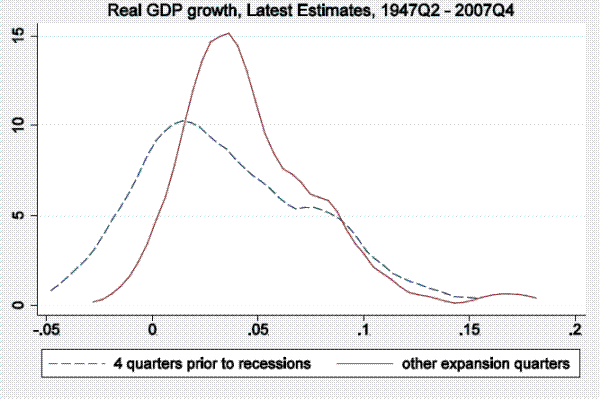
Kernel density estimates for annualized quarterly output growth estimates. The dashed line shows the kernel density fitting the four quarters prior to recessions, while the solid line shows the kernel density fitting all other expansion quarters. The top panel shows density estimates for real GDP growth, the bottom panel for real GDI growth. In both panels, the dashed line is shifted more to the left than the solid line, showing output growth tends to be weaker prior to recessions than in other expansion quarters.
Figure 1B: Kernel Densities, Annualized Quarterly Growth Rates
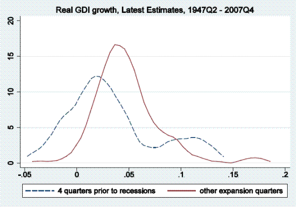
Kernel density estimates for annualized quarterly output growth estimates. The dashed line shows the kernel density fitting the four quarters prior to recessions, while the solid line shows the kernel density fitting all other expansion quarters. The top panel shows density estimates for real GDP growth, the bottom panel for real GDI growth. In both panels, the dashed line is shifted more to the left than the solid line, showing output growth tends to be weaker prior to recessions than in other expansion quarters.
Figure 2A: Output Growth Rates
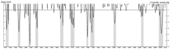
Figure 2B: Output Growth Rates
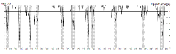
Figure 3A: Kernel Densities, 2-Quarter Annualized Growth
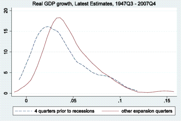
Figure 3B: Kernel Densities, 2-Quarter Annualized Growth
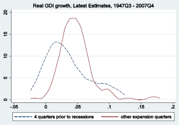
Kernel density estimates for two-quarter annualized output growth estimates. The dashed line shows the kernel density fitting the four quarters prior to recessions, while the solid line shows the kernel density fitting all other expansion quarters. The top panel shows density estimates for real GDP growth, the bottom panel for real GDI growth. In both panels, the dashed line is shifted more to the left than the solid line, showing output growth tends to be weaker prior to recessions than in other expansion quarters.
Figure 4A: Output Growth Rates
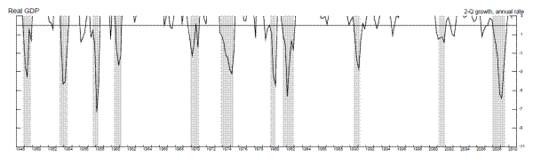
Figure 4B: Output Growth Rates
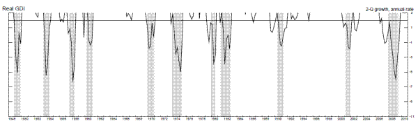
Figure 5A: Kernel Densities, Year-over-Year Growth
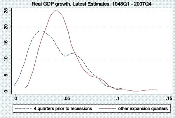
Figure 5B: Kernel Densities, Year-over-Year Growth
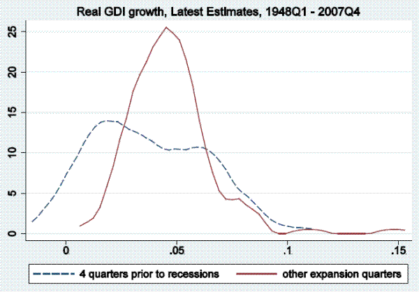
Kernel density estimates for four-quarter annualized output growth estimates. The dashed line shows the kernel density fitting the four quarters prior to recessions, while the solid line shows the kernel density fitting all other expansion quarters. The top panel shows density estimates for real GDP growth, the bottom panel for real GDI growth. In both panels, the dashed line is shifted more to the left than the solid line, showing output growth tends to be weaker prior to recessions than in other expansion quarters.
Figure 6A: Output Growth Rates
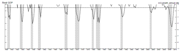
Figure 6B: Output Growth Rates
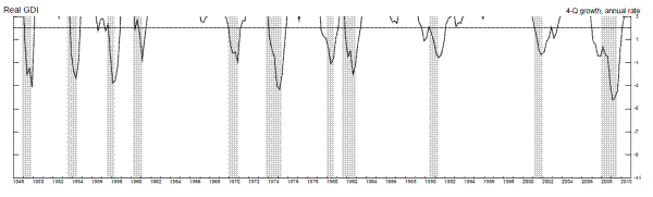
Figure 7: Two-state Markov Switching Models
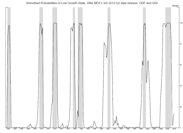
Figure 8: Three-state Markov Switching Model with Stall State
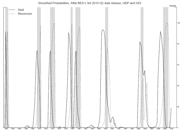
Figure 9A: Three-state Markov Switching Model with Stall State
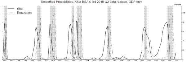
Figure 9B: Three-state Markov Switching Model with Stall State
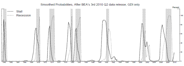
Figure 10A: Three-state Markov Switching Model
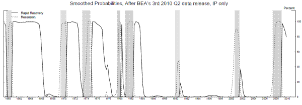
Figure 10B: Three-state Markov Switching Model
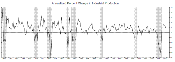
Figure 11A: Three-state Markov Switching Model with Stall State
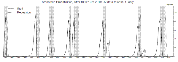
Figure 11B: Three-state Markov Switching Model with Stall State
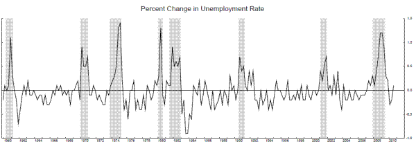
Figure 12A: Three-state Markov Switching Model with Stall State
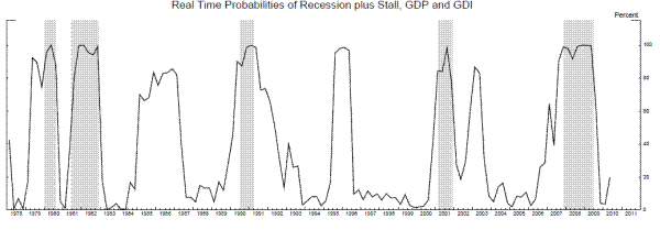
Figure 12B: Three-state Markov Switching Model with Stall State
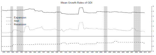
Figure 13: Markov Switching Models
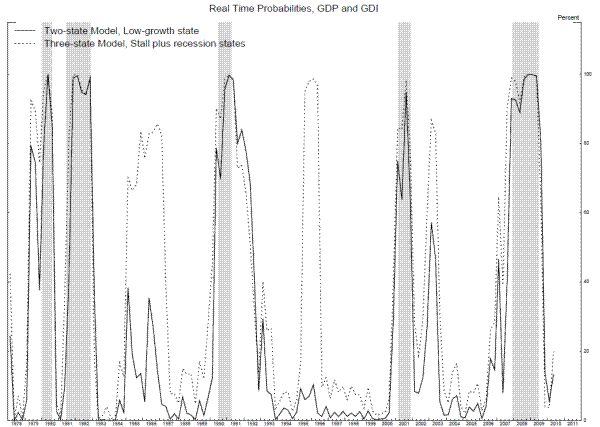
Figure 14A: Three-state Markov Switching Model with Stall State
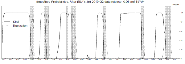
Figure 14B: Three-state Markov Switching Model with Stall State
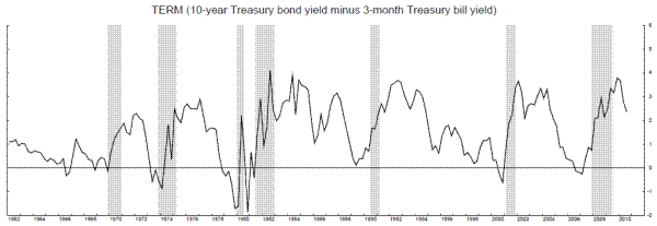
Figure 15A: Three-state Markov Switching Model with Stall State
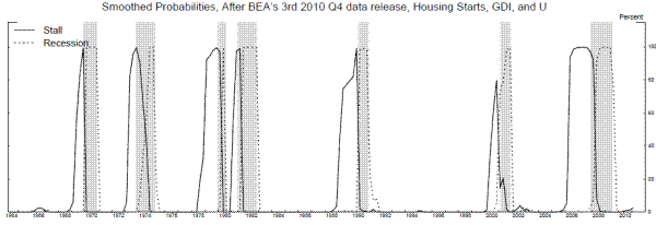
Figure 15B: Three-state Markov Switching Model with Stall State
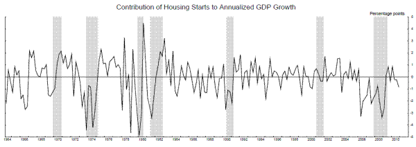
Figure 16A: Three-state Markov Switching Model with Stall State