Skip to: [Printable Version (PDF)] [Bibliography] [Footnotes]

Finance and Economics Discussion Series: 2011-28 Screen Reader version ^♣

Financial Capital and the Macroeconomy:
Policy Considerations*

Michael T. Kiley

Jae W. Sim

Board of Governors of the Federal Reserve System

Keywords: Capital market friction, financial intermediary, capital constraint, Liquidity based asset pricing, asset purchase program, capital injection policy, regulatory capital standards.

Abstract:

We develop a macroeconomic model in which the balance sheet/liquidity condition of financial institutions plays an important role in the determination of asset prices and economic activity. The financial intermediaries in our model are required to make investment commitments before a complete resolution of idiosyncratic funding risk that can be addressed only by costly refinancing, forcing them to behave in a risk-averse manner. The model shows that the balance sheet condition of intermediaries can drive asset values away from their fundamentals, causing aggregate investment and output to respond to shocks to intermediaries. We use this model to evaluate several public policies designed to address balance sheet problems at financial institutions. With regard to short-run policies, we find that capital injections conditioned upon voluntary recapitalization can be a more effective tool than direct lending/asset purchases. With regard to long-run policies, we demonstrate that higher capital requirements can have sizable short-run effects on economic activity if not implemented carefully, and that a long transition period helps avoid such effects.

JEL Classifications: E32, E44, E63.

1 Introduction

To understand the links between financial intermediation and the real economy and to assess related public policies, it is essential to have a model that captures key aspects of the dynamic frictions that cause (at least short-run) deviations from the Modigliani-Miller theorem and hence make the capital structure of the banking sector important for credit provision. These links are thin to non-existent within the workhorse framework for macroeconomic analysis, although research has begun (for instance, Adrian and Shin (2010), Brunnermeier and Pedersen (2009), Gertler and Kiyotaki (2010) and He and Krishnamurthy (2008)). Moreover, banking, finance, and macroeconomics are typically not integrated in the models used in policy circles (e.g., the discussion in Boivin et al. (2010)).

Our goal in this paper is twofold: First, we develop a dynamic model in which the balance sheet/liquidity condition of financial institutions plays an important role in the determination of asset prices and economic activity. Second, using this model, we evaluate the macroeconomic effects of short-term credit policies aimed at stabilizing the balance sheet/liquidity condition of troubled financial institutions, and assess the long-term and transitional effects of implementing higher capital standards. These policies are stylized examples of the types considered in recent discussions.¹

The financial intermediaries in our model are required to make investment commitments before a complete resolution of idiosyncratic funding risk that can be addressed only by costly refinancing (of the type emphasized by, for example, Myers and Majluf (1984) and Bolton and Freixas (2000)). The commitment structure causes financial intermediaries to behave in a risk-averse manner. The resulting caution against taking a large unhedged position given short-run funding uncertainty creates an intermediary specific pricing kernel that can deviate from the stochastic discount factor of a representative household even when the intermediary is fully owned by the household, pushing equilibrium asset returns away from their counterpart in the absence of such intermediation friction, causing aggregate investment and output to respond to shocks to intermediaries.

Our framework yields a highly tractable quantitative framework with which we can assess implications for asset markets and real economic activity. We first show that our model has plausible long-run properties. Shifts in the mix of debt and equity in the capital structure of financial intermediaries are essentially neutral in the long run, as, for example, a shift toward "more expensive" equity is offset by a decline in the borrowing rate (echoing the reasoning in Admati et al. (2010) and Hanson et al. (2011)). In addition, our framework is a business-cycle model that generalizes the LAPM (Liquidity-Based Asset Pricing Model) of Holmström and Tirole (2001), and, as a result, implies a substantial equity premium. The magnitude of this premium can explain almost a half of the measured equity premiums under our baseline calibration, suggesting that incorporation of frictions such as those we consider has important implications beyond our specific focus on the links between the level of capitalization at intermediaries, lending and lending spreads, and real activity.²

In an earlier analysis we illustrated how this model provides realistic responses of macroeconomic variables to financial shocks (Kiley and Sim (2011)), and herein we use the model to assess the efficacy of public policies designed to address balance sheet problems at financial institutions. We consider two types of stabilization policy: direct lending/asset purchase by a public authority and a capital injection conditioned on voluntary recapitalization. Our results indicate that the capital injection policy can be much more powerful than the direct lending/asset purchase policy in stabilizing output fluctuations. In our baseline simulation, the former turns out to be 6 times more effective than the latter in terms of output stabilization effects from interventions of the same size.

The key mechanism behind this difference is that an asset purchase policy suffers from a classic case of crowding out: while aggregate investment is lifted by the increase in government demand, higher government holdings lowers the supply available for private investment. This decrease in supply for private investment boosts asset prices, which causes private demand to decline along the downward sloping demand curve. Overall, the improvement in liquidity conditions and the business environment boosts aggregate demand, but this boost is not enough to overcome the crowding out effect and the size of the stimulative effect dies out rather quickly. In contrast, the capital injection policy increases private demand for capital assets by improving the capital position directly, which boosts the risk appetite for risky assets.³

Finally, we use our model to analyze the transition costs associated with a substantial increase in the minimum capital ratio for banking institutions, a subject that has been the focus of recent debate, as discussed by Admati et al. (2010) and Hanson et al. (2011), but for which a general-equilibrium quantitative assessment has been wanting. Our model fills this gap in quantitative assessments. Though we find the capital structure of the financial sector to be neutral in the long run, shifts in capital requirments can have sizable short-run effects because of the financial frictions facing intermediaries.

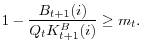
Holding the asset side of the balance sheet constant, raising the regulatory capital ratio increases the probability of costly equity finance since the cash inflow from borrowing has to be reduced to comply with the higher capital constraint. To avoid a stiff rise in the required return on capital, the intermediaries choose to cut back on the asset side of their balance sheet (lending). However, this is costly because the bank earns strictly positive intermediation margins owing to the low cost of funds associated with deposits. Thus, a transition to a higher minimum capital ratio leads financial institutions to balance the marginal cost of issuing equity (reducing dividends) with the marginal cost of cutting back on lending, bringing about a mix of some degree of financial dis-intermediation and bank recapitalization in conjunction with rising lending spreads. As a consequence, the higher capital requirements can have sizable short-run effects on economic activity if not implemented carefully, and a long transition period helps avoid such effects.

2 Model

The model consists of a representative household, a continuum of financial intermediaries, a continuum of competitive final-goods producers, a continuum of competitive investment-goods producers, and a government. The model extends that of Kiley and Sim (2011) through inclusion of a government sector. The following assumptions are central: First, the complexity of the financial markets create prohibitively large transaction costs for households. For this reason, households participate in the financial markets only through financial intermediaries, either in the form of deposits, or in the form of ownership of the intermediaries. Second, households value liquidity services from deposits at financial intermediaries, which implies that households accept returns on intermediary deposits below the risk free rate, creating a strictly positive intermediation margin. Third, the financial intermediaries face capital (margin) constraint in their capital structure choice. The constraint creates an environment where financial intermediaries may not be able to fully arbitrage away all profit opportunities because of the constraint on leverage, and thus leaves a room for policy intervention. We start with the financial intermediaries.

2.1 Financial Intermediaries

2.1.1 Return Structure

A financial intermediary $\in\lbrack0,1]$ purchases capital asset $K_{t+1}^{B}(i)$ at a market price $Q_{t}$ . The intermediary rents out this capital to final-goods firms for net rental incomes defined as

$\displaystyle R_{t+1}^{K}=\tilde{R}_{t+1}^{K}U_{t+1}^{B}(i)-\xi(U_{t+1}^{B}(i))P_{t+1}$

where $\tilde{R}_{t+1}^{K}$ is the nominal rental rate per utilization unit of capital asset ( $K_{t+1}^{B}(i)U_{t+1}^{B}(i)$ ), $U_{t+1}^{B}(i)$ is the utilization rate, $\xi(U_{t+1}^{B}(i))$ is the real cost of utilization and $P_{t+1}$ is the price level of the final goods. Equivalently, the rental income can be thought of as dividends from the final goods firms. In this case, $K_{t+1}^{B}(i)$ should be interpreted as the number of shares. The total return from the investment is composed of rents/dividends ( $R_{t+1} ^{K}K_{t+1}^{B}(i)$ ) and the capital gains associated with the changes in the price of capital assets/shares ( $(1-\delta)Q_{t+1}K_{t+1}^{B}(i)/Q_{t}$ ) where $\delta$ is the depreciation rate of capital.⁴ The superscripts

associated with $K_{t+1}$ and $U_{t+1}$ indicates that the capital stock is owned by a financial intermediary; as discussed below, we also allow the government to own capital assets, denoted by $K_{t+1}^{G}$ . The capital market clearing condition then requires

$\displaystyle 0=K_{t+1}^{G}+\int K_{t+1}^{B}(i)di-K_{t+1}$ for all $\displaystyle t$ .

(1)

To model the balance sheet/liquidity risk that financial intermediaries face, we assume that the rate of return from investment is subject to a multiplicative idiosyncratic shock such that the total rate of return can be decomposed into two components, idiosyncratic and aggregate,

$\displaystyle R_{t+1}^{F}(i)$	$\displaystyle =\epsilon_{t+1}(i)R_{t+1}^{F}$	(2)
	$\displaystyle =\epsilon_{t+1}(i)\left[ \frac{R_{t+1}^{K}+(1-\delta)Q_{t+1}}{Q_{t}}\right]$

where $\epsilon_{t+1}(i)$ is the idiosyncratic component of the return and $R_{t+1}^{F}$ is the aggregate component. We assume that the idiosyncratic shock follows an iid lognormal distribution, $\log\epsilon_{t}(i)\sim N(-0.5\sigma^{2},\sigma^{2})$ .⁵

2.1.2 Capital (Margin) Constraint

To finance the investment described above, the intermediaries mix debt (deposits) and equity. In doing so, they face a capital (margin) constraint, which requires that every dollar of investment asset should be backed by at least $m_{t}$ cents of capital. Denoting the amount of borrowed funds by $B_{t+1}(i)$ , the capital constraint can be stated as

$\displaystyle 1-\frac{B_{t+1}(i)}{Q_{t}K_{t+1}^{B}(i)}\geq m_{t}.$

(3)

A constraint such as the above can arise in various contexts. In Kiley and Sim (2011), we show how such a constraint can be derived from a Value-at-Risk (VaR) constraint such as in Brunnermeier and Pedersen (2009) and Adrian and Shin (2008). In particular, we show that the constraint can arise as a limit point of VaR constraint, where financial intermediaries are never allowed to default, i.e., the intermediaries are always required to raise enough amount of equity capital to stay afloat, a point originally made by Adrian and Shin (2008).⁶ Because our goal is to show the implications of such constraint in an environment where the recapitalization of an intermediary is costly owing to equity market frictions, we avoid the complications associated with endogenously motivating the capital constraint.

In equilibrium, the capital constraint is always binding for two reasons: First, as mentioned before, the household is willing to pay a liquidity premium for its deposits since the intermediary deposits create non-pecuniary returns for the household. Second, even without the liquidity premium, financial intermediaries prefer to issue debt rather than to issue equity owing to the dilution cost associated with equity issuance, which will be explained shortly. As a consequence, the financial intermediaries follow a "pecking order" in their capital structure choice.

2.1.3 Modeling Liquidity Risk

The primary function of financial intermediary is the transformation of short-term liquid assets into long-term illiquid capital assets. Such a transformation exposes the financial intermediaries to liquidity risk. To model this liquidity risk, we adopt the following timing convention for a given period of time :

At the beginning of each period, the aggregate component of returns ( $R_{t}^{F}$ ) becomes known.
After observing the aggregate shocks, the intermediary makes investment ( $Q_{t}K_{t+1}^{B}(i)$ ) and borrowing ( $B_{t+1}(i)$ ) decisions.
After the investment/borrowing decisions are made, the level of the idiosyncratic shock ( $\epsilon_{t}(i)$ ) becomes known to the intermediary and dividend payout /equity issuance decisions ( $D_{t}(i)\gtreqqless0$ ) are made.

The timing convention implies that the financial intermediaries have to make investment commitments before they know their (random) realization of internal funds. It also implies that the revenue shock becomes known only after the borrowing markets for intermediaries are closed. While this precise timing is somewhat arbitrary, it captures important features of reality. In particular, the timing convention represents parsimoniously short-run funding risks. For example, financial intermediaries always face uncertainty about the balance between their short-run loanable funds and/or the cost of such funds in retail/wholesale borrowing markets and the use of outstanding loan commitments; alternatively, realized income can fall short of the funding needs associated with their precommitments due to credit losses or fluctuations in asset values. Under such conditions and when outside equity is more expensive than borrowing, funding uncertainty can make the intermediaries adopt a precautionary stance in making investment/deposit decisions even when all intermediaries are risk-neutral.⁷

2.1.4 Costly Recapitalization

To capture the role of financial market frictions for the intermediaries, we adopt a costly equity finance framework. Owing to the information asymmetry between the intermediaries and the potential owners, equity issuance involves a dilution effect, a phenomenon that a dollar amount of equity issuance reduces the value of existing shares more than a dollar. We operationalize this effect by assuming that the actual cash flow related with equity is given by a function $\varphi(D_{t}(i))$ defined as,

$\displaystyle \varphi(D_{t}(i))$	$\displaystyle =\left\{ \begin{array}[c]{cl} D_{t}(i) & \text{ if }D_{t}(i)\geq0\\ (1-\bar{\varphi})D_{t}(i) & \text{ if }D_{t}(i)<0 \end{array} \right.$
	$\displaystyle =\overset{}{D_{t}(i)-\bar{\varphi}\cdot\min\{D_{t}(i),0\}}.$

In words, when the intermediary pays out a positive amount of dividends, the cash outflow associated with equity is simply given by the dividends payout, $D_{t}(i)$ . However when the intermediary issues new equities ( $D_{t}(i)<0$ ), the cash inflow associated with the notional value $-D_{t}(i)$ is reduced to $-(1-\bar{\varphi})D_{t}(i)$ . Following Bolton and Freixas (2000), we call the foregone cash flow $-\bar{\varphi}D_{t}(i)$ dilution cost .⁸

In each period, financial intermediaries face the following flow of funds constraint,

0	$\displaystyle =$ $\displaystyle \underset{\text{Cash Inflow}}{\underbrace{\epsilon_{t} (i)R_{t}^{F}Q_{t-1}K_{t}^{B}(i)+B_{t+1}(i)}}$	(4)
	$\displaystyle -$ $\displaystyle \underset{\text{Cash Outflow}}{\underbrace{[R_{t}^{B}B_{t} (i)+Q_{t}K_{t+1}^{B}(i)+\varphi(D_{t}(i))]}}.$

The cash inflow is composed of revenue from last period's investment (lending) $\epsilon_{t}(i)R_{t}^{F}Q_{t-1}K_{t}^{B}(i)$ and new borrowing from the household $B_{t+1}(i)$ . The cash outflow consists of repayment to the household for last period's borrowing $R_{t}^{B}B_{t}(i)$ , where $R_{t}^{B}$ is the borrowing rate of the intermediary, and new investment $Q_{t}K_{t+1}^{B}(i)$ . The last item in (4) can be cash inflow or cash outflow depending on the sign of $D_{t}(i)$ . When it is negative, the actual cash inflow is reduced by a constant factor, $\bar{\varphi}$ .⁹ By rearranging the terms and using the definition of capital, the flow of funds constraint can be interpreted as the law of motion for equity capital, i.e.,

$\displaystyle E_{t}(i)=\underset{\text{Net-Worth}}{\underbrace{\text{ }N_{t}(i)\text{ }} }+\underset{\text{Cash Flow for Equity}}{\underbrace{-\text{ }\varphi (D_{t}(i))}}$

where the net-worth of the intermediary is given by

$\displaystyle N_{t}(i)$	$\displaystyle =\underset{}{\epsilon_{t}(i)R_{t}^{F}Q_{t-1}K_{t}^{B}(i)-R_{t} ^{B}B_{t}(i)}$
	$\displaystyle =E_{t-1}(i)+[\epsilon_{t}(i)R_{t}^{F}-1]Q_{t-1}K_{t}^{B}(i)-(R_{t} ^{B}-1)B_{t}(i).$

2.1.5 Value Maximization Problem

To define the optimization problem of an intermediary under the specific timing convention discussed above, it is useful to introduce an expectation operator that accounts for idiosyncratic uncertainty, $\mathbb{E}_{t} ^{i}(\cdot)\equiv\mathbb{E}(\cdot\vert\mathbf{s}_{t}^{A})$ . The conditioning set of the operator includes all aggregate information up to time (denoted by $\mathbf{s}_{t}^{A}$ ) except the current realization of the idiosyncratic shock $\epsilon_{t}(i)$ . We can then formally state the value maximization problem of the intermediary as follows. The intermediary optimizes over $Q_{s}K_{s+1}^{B}(i)$ , $B_{s+1}(i)$ and $D_{s}(i)$ to maximize

$\displaystyle V_{t}^{B}(i)$	$\displaystyle =\max\sum_{s=t}^{\infty}\beta^{s-t}\mathbb{E}_{t}\left[ \frac{\Lambda_{s}}{P_{s}}\mathbb{E}_{t}^{i}[D_{s}(i)]\right]$	(5)
	$\displaystyle +\sum_{s=t}^{\infty}\beta^{s-t}\mathbb{E}_{t}\left\{ \left. \left. \frac{\Lambda_{s}}{P_{s}}\mu_{s}(i)\right[ (1-m_{s})Q_{s}K_{s+1} ^{B}(i)-B_{s+1}^{B}(i)\right] \right\}$
	$\displaystyle +\sum_{s=t}^{\infty}\beta^{s-t}\mathbb{E}_{t}\left\{ \frac{\Lambda_{s} }{P_{s}}\mathbb{E}_{t}^{i}\left[ \underset{}{\lambda_{s}(i)[}\epsilon _{s}(i)R_{s}^{F}Q_{s-1}K_{s}^{B}(i)+B_{s+1}(i)\right. \right.$
	$\displaystyle \left. \left. -R_{s}^{B}B_{s}(i)-Q_{s}K_{s+1}^{B}(i)-\overset{\overset{}{}}{\varphi (D_{s}(i))}]\right] \right\}$

where $\Lambda_{s}$ is the marginal utility of the representative household, $\mu_{s}(i)$ and $\lambda_{s}(i)$ are the Lagrangian multipliers associated with the capital constraint and the flow of funds constraint, respectively.

Note that the intermediary is risk-neutral and discounts the future dividends by the marginal utility of representative household, the owner of the institution. Also note that the flow of funds constraint and its shadow value $\lambda_{s}(i)$ are within the expectation operator $\mathbb{E}_{t}^{i} (\cdot)$ -under our timing assumption, the intermediary has to decide how much to borrow and invest before it comes to know the value of idiosyncratic shock $\epsilon_{s}(i)$ . This implies that the intermediary does not know its own shadow value of internal funds until the idiosyncratic cash flow shock becomes known and the intermediary needs to form an expectation based on aggregate conditions. We can summarize the efficiency conditions of the problem as follows,

FOC for $Q_{t}K_{t+1}(i):$

$\displaystyle \mathbb{E}_{t}^{i}[\lambda_{t}(i)]$ $\displaystyle =\mu_{t}(i)(1-m_{t})$ (6)

$\displaystyle +$ $\displaystyle \beta\mathbb{E}_{t}\left[ \frac{\Lambda_{t+1}}{\Lambda_{t}} \mathbb{E}_{t+1}^{i}[\lambda_{t+1}(i)\epsilon_{t+1}(i)]\frac{R_{t+1}^{F}}{ \Pi_{t+1}}\right]$
FOC for $B_{t+1}(i):$

$\displaystyle \mathbb{E}_{t}^{i}[\lambda_{t}(i)]=\mu_{t}(i)+\beta\mathbb{E}_{t}\left[ \frac{\Lambda_{t+1}}{\Lambda_{t}}\mathbb{E}_{t+1}^{i}[\lambda_{t+1}(i)] \frac{R_{t+1}^{B}}{\Pi_{t+1}}\right]$ (7)
FOC for $D_{t}(i):$

$\displaystyle 1=\overset{}{\lambda_{t}(i)}\varphi^{\prime}(D_{t}(i))$ (8)

where $\Pi_{t+1}\equiv P_{t+1}/P_{t}$ . On the right side of the FOCs for investment and borrowing, all macroeconomic variables at are taken out of the expectation operator $\mathbb{E}_{t+1}^{i}(\cdot)$ , since the conditioning set of $\mathbb{E}_{t+1}^{i}(\cdot)$ includes those variables at time . In contrast, the FOC for dividends is not integrated over the idiosyncratic uncertainty. This is because the dividends/equity financing decisions are made after the realization of the shock.

To see that the capital constraint binds in the steady state, consider the version of (7) that arises in the absence of aggregate uncertainty, i.e., when $\Lambda_{t}=\Lambda_{t+1}$ , $\mathbb{E}_{t}^{i}[\lambda _{t}(i)]=\mathbb{E}_{t+1}^{i}[\lambda_{t+1}(i)]$ , and $\Pi_{t+1}=1$ ,

$\displaystyle 1-\frac{\mu}{\mathbb{E}^{i}[\lambda(i)]}=\beta R^{B}$

Since the idiosyncratic uncertainty does not disappear in the steady state, the shadow value of the flow of funds constraint is still integrated over idiosyncratic uncertainty. Binding capital constraint, i.e., $\mu>0$ requires $\beta R^{B}<1$ . As shown below, this is indeed the case owing to the liquidity premium households place on deposits.¹⁰ By multiplying $1-m_{t}$ to both sides of (7) and subtracting the resulting expression from (6), we can merge the two FOCs into

$\displaystyle m_{t}\mathbb{E}_{t}^{i}[\lambda_{t}(i)]$	$\displaystyle =\beta\mathbb{E}_{t}\left[ \frac{\Lambda_{t+1}}{\Lambda_{t}}\mathbb{E}_{t+1}^{i}[\lambda_{t+1} (i)\epsilon_{t+1}(i)]\frac{R_{t+1}^{F}}{\Pi_{t+1}}\right]$	(9)
	$\displaystyle -\beta\mathbb{E}_{t}\left[ \frac{\Lambda_{t+1}}{\Lambda_{t}} (1-m_{t})\mathbb{E}_{t+1}^{i}[\lambda_{t+1}(i)]\frac{R_{t+1}^{B}}{\Pi_{t+1} }\right]$

This is the version of the efficiency condition that will be used extensively in our analysis that follows. To operationalize (9) for a sharper characterization of the equilibrium, we need to show how the intermediaries in the model form expectations regarding their liquidity condition, which is summarized by two measures, $\mathbb{E}_{t}^{i}[\lambda_{t}(i)]$ and $\mathbb{E}_{t}^{i}[\lambda_{t}(i)\epsilon_{t}(i)]$ .

2.1.6 Intermediary Asset Pricing

Our model has a symmetric equilibrium for three reasons: financial intermediaries are risk-neutral; the first moment of the idiosyncratic shock is time-invariant; and finally, the intermediaries decide how much to invest and to borrow before the realization of their idiosyncratic shocks. In this symmetric equilibrium: all financial intermediaries choose the same level of investment and borrowing, i.e., $K_{t+1}^{B}(i)=K_{t+1}^{B}(j)$ and $B_{t+1}(i)=B_{t+1}(j)$ for all and $j\in\lbrack0,1]$ . This greatly facilitates aggregation. However, dividends/equity issuance decisions are conditioned upon the realization of the idiosyncratic shock. The same thing can be said about the shadow value of the flow of funds constraint, which is the summary measure of the liquidity condition of a particular intermediary.

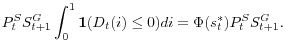
After imposing the binding capital constraint and the symmetric equilibrium condition, we can express the flow of funds constraint as

$\displaystyle D_{t}(i)-\bar{\varphi}\cdot\min\{D_{t}(i),0\}$	$\displaystyle =\epsilon_{t}(i)R_{t} ^{F}Q_{t-1}K_{t}^{B}$
	$\displaystyle -R_{t}^{B}(1-m_{t-1})Q_{t-1}K_{t}^{B}-m_{t}Q_{t}K_{t+1}^{B}.$

At the time of dividend payout/equity issuance decision, all other quantities of the above expression are predetermined. Since the LHS is strictly increasing in $D_{t}(i)$ everywhere, we can find a unique level of the revenue shock that satisfies the flow of funds constraint with $D_{t}(i)=0$ . If we let $D_{t}(i)=0$ and solve for $\epsilon_{t}$ , we obtain an equity financing threshold,

$\displaystyle \epsilon_{t}^{\ast}=(1-m_{t-1})\frac{R_{t}^{B}}{R_{t}^{F}}+m_{t}\frac{1} {R_{t}^{F}}\frac{Q_{t}K_{t+1}^{B}}{Q_{t-1}K_{t}^{B}}.$

If $\epsilon_{t}(i)\geq\epsilon_{t}^{\ast}$ , paying out a strictly positive amount of dividends is optimal while it is optimal to issue equities ( $D_{t}(i)<0$ ), incurring the dilution cost of $\bar{\varphi}$ if $\epsilon_{t}(i)<\epsilon_{t}^{\ast}$ . This and (8) imply that the shadow value of internal funds of the intermediaries depends on the realization of the idiosyncratic shock in the following way:

$\displaystyle \lambda_{t}(i)=1/\varphi^{\prime}(D_{t}(i))=\left\{ \begin{array}[c]{c} 1\\ 1/(1-\bar{\varphi})>1 \end{array} \right. \begin{array}[c]{c} \text{if }\epsilon_{t}(i)\geq\epsilon_{t}^{\ast}\\ \text{if }\epsilon_{t}(i)<\epsilon_{t}^{\ast} \end{array} .$

(10)

The discussion above regarding the equity finance threshold can be used to transform the efficiency condition (9) into a form that is more convenient for a quantitative analysis of the model, which requires us to evaluate two measures of liquidity condition: $\mathbb{E}_{t}^{i}[\lambda_{t}(i)]$ and $\mathbb{E}_{t}^{i}[\lambda_{t}(i)\epsilon_{t}(i)]$ . To that end, let $s_{t}(i)$ be a standardization of $\epsilon_{t}(i)$ defined as

$\displaystyle s_{t}(i)=\sigma^{-1}(\log\epsilon_{t}(i)+0.5\sigma^{2}).$

(11)

Since $s_{t}(i)$ is a monotonic transformation of $\epsilon_{t}(i)$ and follows a standard normal distribution, we can integrate the shadow value over the idiosyncratic uncertainty as follows

$\displaystyle \mathbb{E}_{t}^{i}[\lambda_{t}(i)]$	$\displaystyle =\int_{\epsilon_{t}\geq\epsilon _{t}^{\ast}}1\cdot dF(\epsilon)+\int_{\epsilon_{t}\leq\epsilon_{t}^{\ast} }\frac{1}{1-\bar{\varphi}}\cdot dF(\epsilon)$	(12)
	$\displaystyle =1-\Phi(s_{t}^{\ast})+\frac{\Phi(s_{t}^{\ast})}{1-\bar{\varphi}}=1+ \frac{\bar{\varphi}}{1-\bar{\varphi}}\Phi(s_{t}^{\ast})>1.$

(12) implies that the intermediary's ex ante valuation of a sure dollar is always greater than a dollar as long as the probability of costly recapitalization is strictly positive. What is uncertain here is not the dollar, but its valuation. While the realized shadow value takes only two values: it is either 1 or $1/(1-\bar{\varphi})$ , the expected shadow value is time varying as aggregate conditions change. It is this expected value that matters for the commitment decisions for investment/borrowing. The more likely is costly equity financing, the higher the expected shadow value of internal funds.

To evaluate $\mathbb{E}_{t}^{i}[\lambda_{t}(i)\epsilon_{t}(i)]$ , the following properties of lognormal distribution is useful,¹¹

$\displaystyle \int_{\epsilon\geq\epsilon_{t}^{\ast}}\epsilon f(\epsilon)d\epsilon =[1-\Phi(s_{t}^{\ast}-\sigma)]\int_{0}^{\infty}\epsilon f(\epsilon)d\epsilon,$

where $f(\cdot)$ is the pdf of the lognormal distribution conditioned upon the parameter $\sigma$ and $s_{t}^{\ast}$ is defined as (11). Using properties of the lognormal distribution and noting that $\int_{0}^{\infty }\epsilon f(\epsilon\vert\sigma_{t})d\epsilon=1$ for all bounded positive parameter $\sigma_{t}$ , one can easily see that

$\displaystyle \mathbb{E}_{t}^{i}[\lambda_{t}(i)\epsilon_{t}(i)]$	$\displaystyle =\int_{\epsilon_{t} \geq\epsilon_{t}^{\ast}}\epsilon_{t}dF(\epsilon)+\int_{\epsilon_{t} \leq\epsilon_{t}^{\ast}}\frac{\epsilon_{t}}{1-\bar{\varphi}}dF(\epsilon )$	(13)
	$\displaystyle =1-\Phi(s_{t}^{\ast}-\sigma)+\frac{\Phi(s_{t}^{\ast}-\sigma)} {1-\bar{\varphi}}=1+\frac{\bar{\varphi}}{1-\bar{\varphi}}\Phi(s_{t}^{\ast }-\sigma)>1.$

where $\Phi(s_{t}^{\ast}-\sigma)$ comes from the truncated lognormal distribution.¹² (13) implies that the intermediary's ex ante valuation of a random variable, whose mean is equal to a dollar, is always greater than a dollar. In contrast to the case of $\mathbb{E}_{t}^{i}[\lambda_{t}(i)]$ , what is uncertain is both the cash-flow and its valuation, which makes

$\displaystyle \mathbb{E}_{t}^{i}[\lambda_{t}(i)\epsilon_{t}(i)]$	$\displaystyle =1+\frac{\bar{\varphi} }{1-\bar{\varphi}}\Phi(s_{t}^{\ast}-\sigma)$
	$\displaystyle <1+\frac{\bar{\varphi}}{1-\bar{\varphi}}\Phi(s_{t}^{\ast})$ $\displaystyle =$ $\displaystyle \mathbb{E}_{t}^{i}[\lambda_{t}(i)]$

as long as $\sigma>0$ , reflecting a negative covariance between the shadow value and the idiosyncratic shock in (10). This negative covariance is intuitive - firms with a large positive idiosyncratic shock do not need costly equity financing, and hence have a lower shadow value of internal funds, than do firms with a large negative idiosyncratic shock.

In summary, the caution created by the commitment structure imposed on the investment technology amid unresolved idiosyncratic funding risk manifests itself in the conservative ex ante valuation of random and non-random cash flow. This sets a higher bar for the required return on investment as will be shown below.

Using (12) and (13), we can eliminate all expressions involving the expectation operator $\mathbb{E}_{t}^{i} (\cdot)$ in (9). To that end, it is convenient to rewrite the FOC as

$\displaystyle m_{t}=\beta\mathbb{E}_{t}\left\{ \frac{\Lambda_{t+1}}{\Lambda_{t}}\frac{ \mathbb{E}_{t+1}^{i}[\lambda_{t+1}(i)]}{\mathbb{E}_{t}^{i}[\lambda_{t}(i)]} \left[ \dfrac{\mathbb{E}_{t+1}^{i}[\lambda_{t+1}(i)\epsilon_{t+1}(i)]}{ \mathbb{E}_{t+1}^{i}[\lambda_{t+1}(i)]}\frac{R_{t+1}^{F}}{\Pi_{t+1}} -\left( 1-m_{t}\right) \frac{R_{t+1}^{B}}{\Pi_{t+1}}\right] \right\} .$

Let $\eta\equiv\bar{\varphi}/(1-\bar{\varphi})$ . After dividing the expression through by $m_{t}$ and substituting (12) and (13) in the above, we can derive the intermediary asset pricing formula,

$\displaystyle 1=\mathbb{E}_{t}\left\{ M_{t,t+1}^{B}\left[ \frac{1}{m_{t}}\left( \frac{ \tilde{R}_{t+1}^{F}}{\Pi_{t+1}}-\left( 1-m_{t}\right) \frac{R_{t+1}^{B}}{ \Pi_{t+1}}\right) \right] \right\}$

(14)

where the intermediary's pricing kernel is given by

$\displaystyle M_{t,t+1}^{B}=M_{t,t+1}^{H}\left[ \frac{1+\eta\Phi(s_{t+1}^{\ast})}{ 1+\eta\Phi(s_{t}^{\ast})}\right] =\beta\frac{\Lambda_{t+1}}{\Lambda_{t} }\left[ \frac{1+\eta\Phi(s_{t+1}^{\ast})}{1+\eta\Phi(s_{t}^{\ast})} \right]$

and the risk adjusted return is given as

$\displaystyle \tilde{R}_{t+1}^{F}=R_{t+1}^{F}\left[ \frac{1+\eta\Phi(s_{t+1}^{\ast} -\sigma)}{1+\eta\Phi(s_{t+1}^{\ast})}\right] <R_{t+1}^{F}.$

The above asset pricing formula looks different from a textbook version mainly for two reasons. First, the formula is a levered asset pricing formula. Unlike in the textbook version which assumes away leverage choice, the returns are levered up to the inverse of capital ratio. To see this point, assume $m_{t}=1$ . One can then see that the second term vanish and the formula looks closer to the conventional one, i.e., $1=\mathbb{E}_{t}[M_{t,t+1} ^{B}\cdot\tilde{R}_{t+1}^{F}/\Pi_{t+1}].$

Second, the intermediary specific pricing kernel is a filtered version of the representative household's pricing kernel, where the filter is the ratio of the shadow value of internal funds today vs. tomorrow. The filter could potentially weaken the role of the representative household as a marginal investor even though all financial intermediaries are owned by the households. Suppose that in the beginning of current period, a bad news about aggregate returns arrives. This, holding other things constant, increases the probability of costly recapitalization $\Phi(s_{t}^{\ast})$ since even a normal range of idiosyncratic return may not be enough to meet the funding needs associated with today's investment. If the aggregate shock is strong enough, the ratio of shadow values tomorrow vs. today substantially declines, making overall required return on capital ( $1/M_{t,t+1}^{B}$ ) rise, which suppresses today's investment.

Finally, we note that, when $\bar{\varphi}=0$ , the asset pricing formula collapses to

$\displaystyle 1=\mathbb{E}_{t}\left\{ M_{t,t+1}^{H}\left[ \frac{1}{m_{t}}\left( \frac{ R_{t+1}^{F}}{\Pi_{t+1}}-(1-m_{t})\frac{R_{t+1}^{B}}{\Pi_{t+1}}\right) \right] \right\}$

and idiosyncratic uncertainty plays no role in the determination of asset price. Any arbitrarily large amount of uncertainty simply does not matter for real allocations. In this sense, costly equity finance is the key friction in our framework.

The form of the intermediary asset pricing formula is superficially similar to Jermann and Quadrini (2009), who derive a similar pricing kernel from a reduced-form convex adjustment cost of dividend; however, our approach derives from a specific set of structural frictions. It is also superficially similar to the intermediary asset pricing formula of He and Krishnamurthy (2008); however, they derive their intermediary-specific pricing kernel from the assumption of risk averse intermediaries. The link to the LAPM (Liquidity-Based Asset Pricing Model) of Holmström and Tirole (2001) is more direct: In our case, the liquidity premium arises from costly recapitalization of financial intermediaries, while the premium exists for non-financial corporations with potential investment opportunity or working capital needs in Holmström and Tirole (2001).

2.1.7 Illiquidity of Balance Sheet Assets and Adjustment Cost

In our timing convention, we assume that there exist factors that make the intraperiod adjustment of balance sheet assets difficult, requiring the commitment of participants. In reality, there are also reasons why interperiod as well as intraperiod adjustments of loan portfolio can be costly. As pointed out by many, for instance, Diamond and Rajan (2000), financial assets of intermediaries are inherently illiquid: First, a substantial knowledge about the characteristics of borrowers is an indispensable prerequisite for successful selections of new borrowers and churning out inefficient existing borrowers. Second, a substantial part of balance sheet assets is composed of items that are not easily marketable since the intermediaries cannot commit themselves to work for the second buyers after the sale of such financial assets. Such an illiquidity of balance sheet assets may be the fundamental force behind the slow dynamics often found in balance sheet data.

To capture this aspect in a parsimonious way, we assume that there exists a constant return-to-scale convex adjustment cost associated with changing the nominal stock of financial assets of the intermediaries:

$\displaystyle \gamma(Q_{t-1}K_{t},Q_{t}K_{t+1})=\frac{\bar{\gamma}}{2}\left( \frac {Q_{t}K_{t+1}}{Q_{t-1}K_{t}}-1\right) ^{2}Q_{t-1}K_{t}$ , $\displaystyle \bar{\gamma}\geq0$

With the adjustment friction in balance sheet, it is straightforward to show that the intermediary asset pricing formula is modified into

$\displaystyle 1$	$\displaystyle =\mathbb{E}_{t}\left\{ M_{t,t+1}^{B}\left[ \frac{1}{m_{t}}\left( \frac{\tilde{R}_{t+1}^{F}}{\Pi_{t+1}}-\left( 1-m_{t}\right) \frac {R_{t+1}^{B}}{\Pi_{t+1}}\right) \right] \right\}$	(15)
	$\displaystyle -\frac{\bar{\gamma}}{m_{t}}\left( \frac{Q_{t}K_{t+1}}{Q_{t-1}K_{t} }-1\right) -\mathbb{E}_{t}\left\{ M_{t,t+1}^{B}\frac{\bar{\gamma}}{2m_{t} }\left[ \left( \frac{Q_{t+1}K_{t+2}}{Q_{t}K_{t+1}}\right) ^{2}-1\right] \right\} .$

Though not explicit in (15), the flow of funds constraint and the equity finance threshold need to be modified accordingly as well.

These dynamic costs of adjusting the balance sheet of financial intermediaries are not important for the qualitative predictions of the model, but will help match the dynamics of adjustment apparent in the data.

2.2 Government

Before we describe the other parts of private sector, we discuss the government sector. This makes it easier to explain the household's problem. Because we are only interested in credit policies, our model's government is solely focused on such activities. We consider two types of such credit policy: (i) direct lending/asset purchase policy (ii) capital injection policy. To make the presentation as transparent as possible, we consider one policy at a time.

2.2.1 Direct Lending/Asset Purchase Policy

We first consider a policy under which the government purchases and holds a certain fraction of capital assets for a certain period of time. The policy is motivated by the recognition of the key problem that the financial intermediaries do not have deep pockets under the capital constraint and the costly recapitalization. As a result, at a time when the prices of capital assets are unusually low, the intermediaries cannot sufficiently exploit opportunities for investment that are profitable absent financial frictions, thus intensifying the depth and prolonging the duration of downturns (due to an inability to arbitrage inefficient intermediation wedges, reminiscent of the limits of arbitrage noted by Shleifer and Vishny (1997)). If a third party which does not suffer from the deep pocket problem, say, the government, can intervene and purchase some fraction of capital assets, the undesirable downward spiral between the asset prices and aggregate investment can be mitigated.

Let $S_{t}^{G,K}$ and $S_{t}^{B,K}$ denote the shares of capital assets owned by the government and by the intermediaries, respectively. Using these notations, the market clearing condition for capital assets (1) can be expressed as

$\displaystyle 1=S_{t}^{G,K}+S_{t}^{B,K}.$

We assume that the government does not consider a short-sale policy - e.g., government investment is always greater than or equal to zero, restricting the space of $S_{t}^{G,K}$ to

. We also assume that the government maintains a balanced budget and imposes a lump sum tax to meet the balanced budget constraint,

$\displaystyle T_{t}=Q_{t}S_{t+1}^{G,K}K_{t+1}-R_{t}^{F}S_{t}^{G,K}K_{t}$

(16)

Regarding the budget constraint, three things are important: First, in our analysis, all capital assets are homogeneous by construction. As a result, the issue of potential inefficiency of the government in selecting investment projects is not addressed. Second, the policy can generate profits through the dividends and capital gains channel. Third, the tax policy turns into a transfer policy as the government starts implementing an exit strategy that runs down its investment ( $S_{t+1}^{G,K}<S_{t}^{G,K}$ ).

We assume the following AR(1) process with a serially correlated shock term for the law of motion of the government share $K_{t}^{G}$ ,

$\displaystyle S_{t+1}^{G,K}$	$\displaystyle =\rho_{g}S_{t}^{G,K}+u_{t}^{G,K}$	(17)
$\displaystyle u_{t}^{G,K}$	$\displaystyle =\rho_{u}u_{t-1}^{G,K}+\epsilon_{t}^{G,K}$

The process is effectively an AR(2) process with AR(1) and AR(2) coefficients given by $\rho_{g}+\rho_{u}$ and $-\rho_{g}\rho_{u}$ , respectively. We choose this process to replicate a hump-shaped policy intervention in a parsimonious way: a gradual phase-in and a gradual run-off. Note that the government asset position has a zero steady state and, as mentioned above, we only consider positive values for $S_{t}^{G,K}$ (which places restrictions on the parameters in 17 and the sequence of innovations $\epsilon_{t}^{G,K}$ ).

2.2.2 Capital Injection Policy

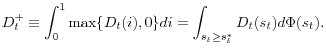
The key friction in our model is the funding risk facing the financial intermediaries because raising outside equity is costly owing to the information problem in equity market. We also have shown that such cost at the aggregate level, denoted by $\Xi_{t}$ , is given by

$\displaystyle \Xi_{t}=-\int_{0}^{1}\bar{\varphi}\min\{D_{t}(i),0\}di.$

Now consider a policy under which the government purchases the shares of the financial intermediaries at market prices and refunds the cost of equity issuance only to the institutions that are raising equities and are owned by the government. Let $S_{t}^{G}(i)$ denote the share of an intermediary owned by the government. With this policy, the market clearing condition of a particular share is given by

$\displaystyle 1=S_{t}^{G}(i)+S_{t}^{H}(i),$

where $S_{t}^{H}(i)$ is the share owned by the households.¹³ Under the proposed policy, the cost of raising equity is reduced to

$\displaystyle \Xi_{t}$	$\displaystyle =-\int_{0}^{1}\bar{\varphi}\min\{D_{t}(i),0\}di+\int_{0}^{1} \bar{\varphi}\min\{D_{t}(i),0\}S_{t+1}^{G}(i)di$
	$\displaystyle =-\int_{0}^{1}\bar{\varphi}\min\{D_{t}(i)[1-S_{t+1}^{G}(i)],0\}di$

Assuming that the government purchases pro rata shares, i.e., $S_{t+1}^{G}(i)=S_{t+1}^{G}$ , the cost can be simplified as

$\displaystyle \Xi_{t}=-(1-S_{t+1}^{G})\int_{0}^{1}\bar{\varphi}\min\{D_{t}(i),0\}di=\bar {\varphi}(1-S_{t+1}^{G})D_{t}^{-}$

where

$\displaystyle D_{t}^{-}\equiv\int_{0}^{1}\min\{D_{t}(i),0\}di=\int_{s_{t}\leq s_{t}^{\ast} }D_{t}(s_{t})d\Phi(s_{t})$

Note that the policy can be seen as equivalent to a subsidy that is proportional to the amount of equity issuance with the subsidy rate given by the government share. Note the role of $\min$ operator in this expression: the financial intermediary is eligible for the subsidy if and only if it is raising outside equity voluntarily.

We assume that the policy is funded by a lump sum tax $T_{t}$ (transfer when negative) of households. Let $P_{t}^{S}(i)$ and $P_{t-1,t}^{S}(i)$ denote the ex-dividend value of equity at time and time value of existing shares outstanding at time , respectively. Assuming a balanced budget in each period, the government budget constraint is given by

$\displaystyle T_{t}$	$\displaystyle =\int_{0}^{1}\mathbf{1}(D_{t}(i)\left. \leq\right. 0)P_{t} ^{S}(i)S_{t+1}^{G}di$
	$\displaystyle -\int_{0}^{1}\mathbf{1}(D_{t-1}(i)\left. \leq\right. 0)[\max \{D_{t}(i),0\}+P_{t-1,t}^{S}(i)]S_{t}^{G}di$

To simplify the budget constraint into a form more convenient for a quantitative analysis, first note that the ex-dividend value of equity $P_{t}^{S}(i)$ is the same for all intermediaries owing to the assumption of iid idiosyncratic shock, i.e., $P_{t}^{S}(i)=P_{t}^{S}\equiv\int_{0}^{1} P_{t}^{S}(i)di$ . To see this point more formally, let $v_{t}^{B}(i)\equiv V_{t}^{B}(i)/\Lambda_{t}$ , the value of an intermediary in real dollar units. The recursive nature of (5) implies that the following Bellman equation holds,

$\displaystyle v_{t}^{B}(i)=d_{t}(i)+\mathbb{E}_{t}[M_{t,t+1}^{H}\cdot\mathbb{E} _{t+1} ^{i}[v_{t+1}^{B}(i)]]$

where $d_{t}(i)\equiv D_{t}(i)/P_{t}$ . Let $v_{t}^{B}\equiv\mathbb{E}_{t} ^{i}[v_{t}^{B}(i)]=\int_{0}^{1}v_{t}^{B}(i)di$ , the aggregate value of all intermediaries at time

. This is also the expected value of an individual intermediary before the realization of the idiosyncratic shock. The ex-dividend value of equity at time

, $P_{t}^{S}(i)$ is given by $P_{t}\mathbb{E}_{t}[M_{t,t+1}^{H}\cdot v_{t+1}^{B}]$ and hence is the same for all intermediaries. Hence, the first term on the RHS of the budget constraint is equivalent to

$\displaystyle P_{t}^{S}S_{t+1}^{G}\int_{0}^{1}\mathbf{1}(D_{t}(i)\left. \leq\right. 0)di=\Phi(s_{t}^{\ast})P_{t}^{S}S_{t+1}^{G}.$

Also note that by the assumption of iid idiosyncratic shock and the law of large number, we have

	$\displaystyle \int_{0}^{1}\mathbf{1}(D_{t-1}(i)\left. \leq\right. 0)[\max\{D_{t} (i),0\}+P_{t-1,t}^{S}(i)]di$
	$\displaystyle =\Phi(s_{t-1})\int_{0}^{1}[\max\{D_{t}(i),0\}+P_{t-1,t}^{S}(i)]di$

In words, the partial sums of the dividends and current values of existing shares of the intermediaries that issued new shares at time

are the same as the total sums multiplied by the measure of such intermediaries.

We can then simplify the budget constraint as

$\displaystyle T_{t}=\Phi(s_{t})P_{t}^{S}S_{t+1}^{G}-\Phi(s_{t-1})(D_{t}^{+}+P_{t-1,t} ^{S})S_{t}^{G}$

where

$\displaystyle D_{t}^{+}\equiv\int_{0}^{1}\max\{D_{t}(i),0\}di=\int_{s_{t}\geq s_{t}^{\ast} }D_{t}(s_{t})d\Phi(s_{t}).$

and $P_{t-1,t}^{S}\equiv\int P_{t-1,t}^{S}(i)di$ . As mentioned above, the government purchases only the shares of the institutions that are issuing new equities, which explains the presence of $\Phi(s_{t})$ in the first term of the budget constraint. Under the assumption of no persistence in the first moment of the idiosyncratic shock and by the law of large numbers, the government portfolio held in time

shares all the properties of the aggregates at time

. This explains why we can simply multiply $\Phi (s_{t-1})$ to the second term without having to keep track of the identities (or the distribution) of the intermediaries that issued new shares at time

The last two remarks for the direct lending/asset purchase policy can be applied here as well: the government can earn profits during the implementation of the policy and the tax policy turns into a transfer policy once the exit strategy ( $S_{t+1}^{G}<S_{t}^{G}$ ) kicks in. For a straightforward comparison of this policy with direct lending/asset purchase policy, we specify exactly the same process as in the latter case,

$\displaystyle S_{t+1}^{G,S}$	$\displaystyle =\rho_{g}S_{t}^{G,S}+u_{t}^{G,S}$	(18)
$\displaystyle u_{t}^{G,S}$	$\displaystyle =\rho_{u}u_{t-1}^{G,S}+\epsilon_{t}^{G,S}$

Again, to ensure that such policy does not affect the long run equilibrium of the economy, we set the steady state of the government share equal to zero. We then perform the same perfect foresight deterministic simulation to ensure that $S_{t}^{G}$ does not go outside the proper range,

2.3 Household

The representative household consumes the final-goods and earns market wages by supplying labor inputs for the production of final goods. We assume that the household lacks necessary skills to directly manage investment projects. For this reason, the household invests its saving through financial intermediaries. The household can either invest in the shares of the intermediaries or make deposits to the intermediaries.

2.3.1 Budget Constraint

Under the assumptions made above, the budget constraint of the representative household can be expressed as

0	$\displaystyle =W_{t}H_{t}+R_{t}^{B}B_{t}-P_{t}C_{t}-T_{t}- \int_{0}^{1}P_{t} ^{S}(i)S_{t+1}^{H}(i)di$	(19)
	$\displaystyle -B_{t+1}+\int_{0}^{1}[\max\{D_{t}(i),0\}+P_{t-1,t}^{S}(i)]S_{t} ^{H}(i)di$

where $B_{t}=\int B_{t}(i)di$ , $W_{t}$ is a nominal wage rate, $H_{t}$ is labor hours, $T_{t}$ is the lump sum tax and $S_{t}^{H}(i)$ is the number of shares owned by the households outstanding at time

Consider an accounting identity that relates the ex-dividend value of equity at time ( $P_{t}^{S}(i)$ ) to the time value of existing share outstanding at time :

$\displaystyle P_{t}^{S}(i)=P_{t-1,t}^{S}(i)+X_{t}(i)$

where $X_{t}(i)$ is the value of new shares. The dilution effect discussed in the intermediary problem implies that the value of new shares, absent any public intervention, is given by the amount of negative dividends reduced by a dilution factor $\bar{\varphi}$ ,

$\displaystyle X_{t}(i)=-(1-\bar{\varphi})\min\{D_{t}(i),0\}.$

The value of new shares under the capital injection policy is modified into

$\displaystyle X_{t}(i)=-(1-\bar{\varphi})\min\{D_{t}(i),0\}-\bar{\varphi}\min\{D_{t} (i),0\}S_{t+1}^{G}$

As a result, holding the value of outstanding share at time

( $P_{t-1,t}^{S}(i)$ ) constant, the capital injection policy increases the ex-dividend value of equity at time

exactly by $-\bar{\varphi}\min \{D_{t}(i),0\}S_{t+1}^{G}$ , i.e.,

$\displaystyle P_{t}^{S}(i)=P_{t-1,t}^{S}(i)-[1-(1-S_{t+1}^{G})\bar{\varphi}]\min \{D_{t}(i),0\}.$

(20)

Substituting the accounting identity (20) in (19), one can see that the budget constraint is equivalent to

0	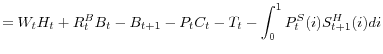$\displaystyle =W_{t}H_{t}+R_{t}^{B}B_{t}-B_{t+1}-P_{t}C_{t}-T_{t}-\int_{0}^{1}P_{t} ^{S}(i)S_{t+1}^{H}(i)di$	(21)
	$\displaystyle +\int_{0}^{1}[\max\{D_{t}(i),0\}+[1-(1-S_{t+1}^{G})\bar{\varphi}]\min \{D_{t}(i),0\}+P_{t}^{S}(i)]S_{t}^{H}(i)di$

2.3.2 Preferences

For the preferences of the representative household, we adopt the most standard specifications for quantitative analyses in the literature. One such specification can be found in Smets and Wouters (2007). More specifically, we adopt an internal habit in consumption and a labor disutility separable from the utility of consumption. To model the value households place on their deposits, we adopt the deposit-in-the utility specification originating from Sidrauski (1967), which captures the non-pecuniary benefits provided by financial institutions.¹⁴ Formally, the preferences are given by

$\displaystyle u(C_{t},C_{t-1},B_{t+1}/P_{t},H_{t})$	$\displaystyle =\log(C_{t}-aC_{t-1})$	(22)
	$\displaystyle -$ $\displaystyle \frac{\zeta}{1+\psi}(H_{t})^{1+\psi}+$ $\displaystyle \theta\log\left( \int\frac{B_{t+1}(i)}{P_{t}}di\right) .$

The household problem is straightforward: the household chooses $\{C_{t}$ , $H_{t}$ , $B_{t+1}(i)$ , $S_{t}(i)\}$ to maximize its value,

$\displaystyle V_{t}^{H}=\max\sum_{s=t}^{\infty}\beta^{s-t}\mathbb{E}_{t}u(C_{s} ,C_{s-1},B_{s+1}/P_{s},H_{s})$

subject to the budget constraint (21). For later purpose, let $\Lambda_{t}$ denote the Lagrangian multiplier associated with the budget constraint (21).

2.3.3 Pricing Financial Intermediaries

We now show how the representative household prices the debts and equities of the financial intermediaries. The FOCs for consumption, deposits and shares are given by

FOC for $C_{t}:$

$\displaystyle \Lambda_{t}=\frac{1}{C_{t}-aC_{t-1}}-\beta\mathbb{E}_{t}\left[ \frac{a}{ C_{t+1}-aC_{t}}\right]$ (23)
FOC for $B_{t+1}(i):$

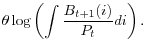
$\displaystyle 1=\frac{\theta/\Lambda_{t}}{B_{t+1}(i)/P_{t}}+\beta\mathbb{E}_{t}\left[ \frac{\Lambda_{t+1}}{\Lambda_{t}}\frac{R_{t+1}^{B}}{\Pi_{t+1}}\right]$ (24)
FOC for $S_{t+1}^{H}(i):$

$\displaystyle P_{t}^{S}(i)$ $\displaystyle =\beta\mathbb{E}_{t}\left\{ \frac{\Lambda_{t+1}}{\Lambda_{t} }\mathbb{E}_{t+1}^{i}[\max\{D_{t+1}(i),0\}\right.$ (25)

$\displaystyle \left. \underset{}{\overset{}{+[1-(1-S_{t+2}^{G})\bar{\varphi} ]\min\{D_{t+1}(i),0\}+P_{t+1}^{S}(i)]}}\right\}$

The FOC for consumption is standard. The FOC for intermediary debt is different from a standard asset pricing formula because of the non-pecuniary benefit of deposit. This creates a liquidity premium that the household is willing to fore-go in making deposits at a rate lower than risk-free rate. Formally, the liquidity premium can be defined as

$\displaystyle \beta\mathbb{E}_{t}\left[ \frac{\Lambda_{t+1}}{\Lambda_{t}}\left( \frac{R_{t+1}}{\Pi_{t+1}}-\frac{R_{t+1}^{B}}{\Pi_{t+1}}\right) \right] =\frac{\theta/\Lambda_{t}}{B_{t+1}(i)/P_{t}}\geq0$

where $R_{t+1}$ is a risk-free rate that satisfies the fictitious asset pricing equation, $1=\beta\mathbb{E}_{t}[(\Lambda_{t+1}/\Lambda_{t} )(R_{t+1}/\Pi_{t+1})]$ . In the non-stochastic steady state, we have $1=\beta R$ and

$\displaystyle \frac{\theta/\Lambda}{B/P}=1-\beta R^{B},$

which implies that $\beta R^{B}\leq1$ with the inequality strict if $\theta >0$ . This proves the statement that the capital constraint binds for the intermediaries in the steady state.

2.3.4 Cost of Capital

From a theoretical perspective, the relevant cost of capital for a financial intermediary is a marginal cost (or a weighted average of marginal costs), as can be seen directly by rewriting (9) as

	$\displaystyle \overset{}{\underset{\text{MB of Investment}}{\underbrace{\mathbb{E} _{t}\{M_{t,t+1}^{H}\mathbb{E}_{t+1}^{i}[\lambda_{t+1}(i)\epsilon _{t+1}(i)]R_{t+1}^{F}\}}}}$
	$\displaystyle =\underset{\text{MC of Investment}}{\underbrace{m_{t}\mathbb{E} _{t} ^{i}[\lambda_{t}(i)]+(1-m_{t})\mathbb{E}_{t}\left\{ M_{t,t+1}^{H} \mathbb{E}_{t+1}^{i}[\lambda_{t+1}(i)]\frac{R_{t+1}^{B}}{\Pi_{t+1}} \right\} }}.$	(26)

The above equates the marginal benefit (LHS) and the marginal cost (RHS) of investment. Evidently it is an weighted average of two components, the one associated with the marginal cost of raising capital and the one associated with marginal borrowing cost.

If the marginal cost of capital is constant, the distinction between marginal and average costs of capital is meaningless unless there is a fixed cost component, which is absent in our environment. One might be tempted to take this conclusion given that the per-unit cost of issuing equity is constant and the retail borrowing market is competitive. However, the marginal cost of capital is increasing in the size of the balance sheet. To see this point, remember that the equity financing threshold is given by

$\displaystyle \epsilon_{t}^{\ast}=(1-m_{t-1})\frac{R_{t}^{B}}{R_{t}^{F}}+m_{t}\frac{1} {R_{t}^{F}}\frac{Q_{t}K_{t+1}^{B}}{Q_{t-1}K_{t}^{B}}.$

The threshold is increasing in the size of balance sheet, $Q_{t}K_{t+1}^{B}$ : the greater the size of the balance sheet, the more likely to face the recapitalization problem. Also remember that the expected shadow value is increasing in the threshold, $\mathbb{E}_{t}^{i}[\lambda_{t}(i)]=1+\eta \Phi\lbrack(\log\epsilon_{t}^{\ast}+0.5\sigma^{2})/\sigma]$ . We can then consider a thought experiment in which the size of the balance sheet is permanently increased, boosting $Q_{t}K_{t+1}^{B}$ today and $Q_{t+1} K_{t+2}^{B}$ tomorrow in the same proportion. Holding the asset return and borrowing rate constant, this increases the equity finance threshold $\epsilon_{t}^{\ast}$ and the probability of costly recapitalization today, and causes the marginal cost of capital to rise, implying a convex cost of capital.

While the marginal cost is the theoretically valid concept for capital budgeting, often policy debates have centered around a slightly different concept of cost of capital: the weighted average cost of capital (WACC). This concept has played a significant role in assessments of the economic impact of changes in regulatory regime for capital standards, under the (potentially naive) view that equity is more costly than debt. For example, some assessments of the economic impact of shifts in required capital starts with an estimate of the effect on the weighted average cost of capital for financial institutions (see for instance BIS (2010a) and BIS (2010b)). The advantage of such a concept is its observability. In this subsection, we show how such an observable measure of cost of capital can be constructed.

The weighted average cost of capital $R_{t+1}^{W}$ is defined as the weighted sum of returns on equity and debt, i.e.,

$\displaystyle \mathbb{E}_{t}R_{t+1}^{W}=m_{t}\mathbb{E}_{t}R_{t+1}^{S}+\left( 1-m_{t}\right) R_{t+1}^{B}.$

(27)

Hence, the key issue in constructing the cost of capital is how to measure the return on equity, especially when the issuer faces costly equity financing friction. The household FOC for share can be used for this purpose. To that end, first remember that $P_{t}^{S}(i)=P_{t}^{S}$ for all

, and trivially, $\mathbb{E}_{t+1}^{i}[P_{t+1}^{S}(i)]=P_{t+1}^{S}$ . Noting that $\mathbb{E} _{t+1}^{i}[\max\{D_{t+1}(i),0\}]=D_{t+1}^{+}$ , $\mathbb{E}_{t+1}^{i} [\min\{D_{t+1}(i),0\}]=-D_{t+1}^{-}$ and $D_{t+1}=D_{t+1}^{+}-D_{t+1}^{-}$ , we can rewrite the asset pricing formula (25) as

$\displaystyle 1$	$\displaystyle =\beta\mathbb{E}_{t}\left\{ \frac{\Lambda_{t+1}}{\Lambda_{t}}\left[ \left( \frac{D_{t+1}+P_{t+1}^{S}}{P_{t}^{S}}\right) +\bar{\varphi} (1-S_{t+2}^{G})\frac{D_{t+1}^{-}}{P_{t}^{S}}\right] \right\}$
	$\displaystyle \equiv\beta\mathbb{E}_{t}[M_{t,t+1}^{H}\cdot R_{t+1}^{S}]$	(28)

The first component of return on equity is conventional: the return on equity is the sum of dividend/price ratio and the capital gain. The second component is the direct result of costly equity financing assumption we adopt. From the formula (28), one can easily see how the costly equity finance increases the cost of equity. One can also see how the capital injection policy directly lowers the cost of equity, and hence, the weighted cost of capital.

2.4 Technology

To save space, our description of the rest of the model economy will be brief. Our goal in this analysis is to investigate the role of funding-market frictions facing financial intermediaries and to consider the effects of unconventional public policies designed to address balance-sheet strains at financial institutions in an environment where other policy tools (such as traditional monetary policy) are not available. For this reason, we take the model as close as possible to a real business cycle benchmark. While we keep distinctions between nominal and real variables in our notation (thereby allowing easy integration of monetary policy questions at a later stage), price adjustment is frictionless in this analysis.

2.4.1 Final Goods

A continuum of competitive firms produce final goods using capital and labor in a constant return-to-scale (CRS) Cobb-Douglas technology. They solve the following static profit maximization problem,

$\displaystyle \max_{K_{t}(j)U_{t}(j),H_{t}^{H}(j)}\{P_{t}Z_{t}(K_{t}(j)U_{t}(j))^{1-\alpha }H_{t}^{H}(j)^{\alpha}-W_{t}H_{t}(j)-R_{t}^{K}(K_{t}(j)U_{t}(j))\}$

where $Z_{t}$ is an aggregate technology shock. Since the scale of the problem is indeterminate, one could assume a representative firm instead of a continuum.

2.4.2 Investment

A continuum of competitive firms produce investment goods by combining an input of final goods and a CRS adjustment technology. Following Christiano et al. (2003) and Smets and Wouters (2007), we specify a convex investment adjustment cost and model the investment problem as follows,

$\displaystyle V_{t}^{I}=\max_{I_{s}(k)}\mathbb{E}_{t}\sum_{s=t}^{\infty}\beta^{t-s}\frac{ \Lambda_{s}}{P_{s}}\left\{ Q_{s}I_{s}(k)-P_{s}\left[ I_{s}(k)+\frac{\bar{ \chi}}{2}\left( \frac{I_{s}(k)}{I_{s-1}(k)}-1\right) ^{2}I_{s-1}(k)\right] \right\} .$

Again, the problem is scale-free and can be thought of as the one of a representative firm instead of a continuum.

2.4.3 Goods Market Clearing Condition

The goods market clearing condition of the model economy is given by

$\displaystyle Y_{t}=C_{t}+I_{t}+\frac{\bar{\chi}}{2}\left( \frac{I_{t}-I_{t-1}}{I_{t-1} }\right) ^{2}I_{t-1}+\frac{\bar{\tau}}{2}\left( \frac{Q_{t}K_{t+1}} {Q_{t-1}K_{t}}\Pi_{t}-1\right) ^{2}\frac{Q_{t-1}K_{t}}{\Pi_{t}}.$

(29)

Note the absence of financial flows related with equity issuance costs and government subsidy for equity issuance. This is due to our assumption that the dilution cost of equity issuance takes the form of discount sale, rather than an efficiency loss for the economy (see the appendix in the working paper version for a detailed derivation for the goods market clearing condition).

3 Long Run Effects of Capital Constraint

In this section, we use some comparative statics and simulation exercises to analyze the effects of capital market frictions such as capital constraint and costly equity finance on the equilibrium returns and capital accumulation in the long run. In particular, considering the ongoing debate on the long-run effects of regulation on capital standards, we pay a special attention to the long-run effects of alternative levels of capital constraints.

3.1 Equilibrium Return Premium

In this subsection, we show how the changes in model parameters related with the degree of funding-market frictions affect the return premium and capital accumulation. To that end, we start with the steady-state version of the investment Euler equation of the model. In the steady state, the FOC for investment, equation (14), takes the form of

$\displaystyle m/\beta+(1-m)R^{B}=\left[ \frac{1+\eta\Phi\left( s^{\ast}-\sigma\right) }{1+\eta\Phi\left( s^{\ast}\right) }\right] \cdot R^{F}.$

(30)

To interpret the economic contents of the expression, it is useful to note that the stock market return of intermediary (28) is equalized to $1/\beta$ in the steady state if and only if $\eta=\bar{\varphi} /(1-\bar{\varphi})=0$ since, with no aggregate uncertainty and $\bar{\varphi}=0$ , $R^{S}=v^{B}/(m^{H}\cdot v^{B})=1/\beta$ . Therefore, one can think of the left side of (30) as the frictionless weighted average cost of capital.¹⁵ Let us denote this by $R^{W\ast}$ . We can then see immediately

$\displaystyle \frac{R^{W\ast}}{R^{F}}=\left[ \frac{1+\eta\Phi\left( s^{\ast} -\sigma\right) }{1+\eta\Phi\left( s^{\ast}\right) }\right] =\frac {\mathbb{ E}^{i}[\lambda(i)\epsilon(i)]}{\mathbb{E}^{i}[\lambda(i)]} \leq1.$

(31)

From a mechanical standpoint, the inequality is due to the monotonicity of the standard normal distribution. From an economic standpoint, however, the inequality is the result of the negative correlation between the shadow value of internal funds and the idiosyncratic profitability shock, which would not exist if the funding market were frictionless ( $\bar{\varphi}=0$ ). Facing costly recapitalization risk, the intermediaries adopt a cautionary stance before they enter commitments, reducing the investment level ex ante. As a result, given the diminishing marginal productivity of capital, the return on assets $R^{F}=r^{K}+1-\delta$ cannot come down to the level of the frictionless cost of capital despite the competitive structure and free entry in the financial industry. Obviously this is the direct result of the costly equity financing assumption. We call the bracketed term the intermediation wedge.

The intermediation wedge plays an important role in the determination of excess returns of the risky asset. To see this, we can rewrite (30 ) as

$\displaystyle R^{F}-R=R^{W\ast}\cdot\left[ \frac{1+\eta\Phi\left( s^{\ast}\right) }{ 1+\eta\Phi\left( s^{\ast}-\sigma\right) }\right] -R$

(32)

Two things stand out from this expression. First, in our model economy, an equity premium can exist in a non-stochastic steady state. The premium arises not because of the covariance of asset return and the pricing kernel of the representative household, but because of the frictions in funding markets for the financial intermediaries. In essence, the premium is closer to the liquidity premium in the LAPM (Holmström and Tirole (2001)) since it is the short-run funding risk associated with idiosyncratic return uncertainty that generates such a wedge.

Second, in the special case of $\theta=0$ (no deposits in the utility), $R^{W\ast}=1/\beta$ since $R^{B}=R$ . In this extreme case, the risk premium is entirely determined by the intermediation wedge and is always strictly positive as long as idiosyncratic uncertainty exists. It is possible, though not plausible in a realistic calibration, that the premium can be negative. This happens when $R^{W\ast}$ is too low relative to risk free rate . For instance, if the non-pecuniary benefit of deposit is pathologically large, it is possible that the household is willing to make deposit at a negative net interest rate, i.e., $R^{B}<1$ . In this case, the product of $R^{W\ast}$ and the inverse of the intermediation wedge can be smaller than the rate of time preference, implying a negative premium. The same situation can also happen when the idiosyncratic uncertainty is sufficiently low. In this case, the intermediation wedge is close to 1 and the right side of (32) can be negative since $R^{W\ast}\leq1/\beta$ . However, as will be shown below, such extreme cases do not happen with realistic calibrations.

An empirically relevant question is if the model can generate a sizable equity premium with a realistic calibration through the liquidity channel. Two crucial parameters are the dilution cost parameter $\bar{\varphi}$ , also known as floatation cost, and the amount of idiosyncratic uncertainty $\sigma$ . Figure 1 depicts the relationship between the idiosyncratic uncertainty and the equity premium for a range of parameter values for equity issuance cost. Evident are the positive relationship between the uncertainty and the return premium on one hand, and the positive relationship between the equity issuance cost and the return premium on the other hand.

These are not surprising given the theoretical structure we adopt. What is interesting is the magnitude of return premium created by the capital market frictions. There exists a wide range of the dilution cost parameter in the literature. For instance, Gomes (2001) reports 0.08 of per-unit equity issuance cost. Recently Hennessy and Whited (2007), using simulated methods of moments, provides the structural estimates of issuance cost function; their estimates of the total cost, including fixed and variable costs, is somewhat higher than reported by Gomes (2001). Cooley and Quadrini (2001) use 0.30 for their analysis, which we take for our baseline case. While this calibration is on the high end, this level of dilution cost is appropriate for the analysis of the effects of liquidity policies designed to cope with crisis situation; moreover, the empirical analysis in Kiley and Sim (2011) suggests this value helps fit the data on macroeconomic/financial interactions along some dimensions (see below). For the variance of idiosyncratic shocks, or riskiness measure, of the financial intermediaries, we choose $\sigma=0.10$ in annual frequency for our baseline calibration.

Figure 1 shows that the model generates a sizable range of return premium at plausible levels of uncertainty as long as the dilution cost is greater 0.15. At our baseline calibration, the model creates a return premium of about 300 basis points. When the dilution cost is 0.20, the model generates a 200 basis points premium. Given our conservative calibration of the uncertainty level, one can see that the model can explain a substantial part of the equity premium through the capital market frictions facing financial intermediaries.

3.2 Near Long Run Neutrality of Capital Constraint

In policy circles, it is often emphasized that a higher minimum capital ratio may increase the weighted average cost of capital for financial intermediaries in the long run. This is because the minimum capital regulation changes the mix of debt and equity so as to make financial institutions more reliant on the costly equity funding (e.g., BIS (2010a) and BIS (2010b)). However, such a conclusion does not consider potential general equilibrium effects. With a higher level of capital, financial intermediaries issue less amount of debts (or deposits) for a given level of lending. For this to happen in general equilibrium, the representative household should be discouraged from holding intermediary deposits, which occurs through a lower return on such deposits and hence a lower borrowing rate for the intermediaries. This counteracts the partial equilibrium tendency of the effective cost of capital for the intermediaries to rise from greater reliance on equity.¹⁶

To analyze the general equilibrium effects in detail, we need to show how the deposit rate and return on assets are jointly determined in equilibrium. To that end, we derive a relationship between the deposit rate and return on asset that clears the goods market. We then combine this condition with the financial market equilibrium condition given by (30) to find the set of rates of returns that support equilibrium in both markets. By using the two FOCs of the household for consumption and deposits, one can derive a linear relationship between consumption and deposit,

$\displaystyle c$	$\displaystyle =\frac{(1-a\beta)(1-\beta R^{B})}{(1-a)\theta}b$
	$\displaystyle =\frac{(1-a\beta)(1-\beta R^{B})(1-m)}{(1-a)\theta}k$

where the second equality is from the binding capital constraint. Here we use lower case letters for real quantities in the long run. From the rental market equilibrium condition, we have

$\displaystyle \frac{y}{k}=\frac{R^{F}-(1-\delta)}{1-\alpha}$

Substituting the two expressions in the resource constraint $y/k=c/k+\delta$ , one can derive a linear relationship that $R^{F}$ and $R^{B}$ have to jointly satisfy,

$\displaystyle \frac{R^{F}-(1-\delta)}{(1-\alpha)}=\frac{(1-a\beta)(1-\beta R^{B} )(1-m)}{(1-a)\theta}+\delta.$

(33)

We can then numerically solve the non-linear simultaneous equations system of (30) and (33) to determine $R^{E}$ and $R^{B}$ .

Figure 2 shows the determination of two steady states, one with and the other with . The red solid line shows the linear relationship between $R^{F}$ and $R^{B}$ that satisfy (33) (the real side of equilibrium) when .¹⁷ The blue solid line presents the locus of $R^{F}$ and $R^{B}$ that satisfy the financial side of equilibrium, i.e., (30) when . Evident is that the locus has a steep upward slope: when the borrowing rate for the financial intermediaries go up, the return on asset also has to go up to create an enough incentive for the intermediaries to invest. Point A is the intersection of the two loci, displaying the initial long run equilibrium when .

In the figure, we perform a thought experiment in which the minimum capital ratio is raised up to 0.25 and show how a new long-run equilibrium is determined. When the capital ratio goes up, the financial locus shifts downward with a steeper slope between the borrowing rate and the asset return (the blue dotted line): with a much higher minimum capital ratio, the weighted average cost of capital goes up since the new regulation forces the financial intermediaries to change a substantial portion of funding source from relatively cheap debts/deposits to more expensive equity. As a result, the investment in capital assets declines and the asset return goes up. The economy moves to point B. However, B cannot be an equilibrium because the real side of the equilibrium also changes. A new equilibrium requires the intermediaries to reduce the borrowing level substantially. The only way for the economy to achieve this is to discourage the households to hold intermediary debt/deposits: the borrowing rate for intermediaries (e.g., the deposit rate in our simple model) has to go down. The locus $R^{F}$ and $R^{B}$ that satisfy the real side of equilibrium shifts down to a new one (the red dotted line) and the new equilibrium is found at point C.

Whether the return on asset is higher or lower than the initial value depends on how sensitive this downward shift is. It turns out that the capital constraint in our model economy is near neutral: the shift in the red line almost perfectly offsets the movement in the blue line. For instance when the economy moves from to , the equilibrium asset returns drops less than 0.2 bps at an annual rate.

This thought experiment shows how the capital constraint is nearly neutral for real outcomes in the long run; this echoes the conventional wisdom, due to "Modigliani-Miller" type effects, in related academic research (e.g. Admati et al. (2010) and Hanson et al. (2011)). The near-neutrality of capital constraint, however, does not mean that a transition from one equilibrium to another will be costless. The short-run transitional dynamics is a totally different issue, to which we turn later in our analysis.

4 Policy Experiments

In this section, we consider the effects of various government policies to improve financial stability. We start by assigning parameter values. We then consider the efficacy of unconventional short-term credit policies designed to cope with extraordinary and exigent circumstances. We close the section by analyzing the transitional dynamics of the economy moving from one steady state to another under the proposed higher capital standards.

4.1 Calibration

There are three parameters that govern key aspects of the model's predictions for the macroeconomic effects of credit policies: the cost of equity issuance $\bar{\varphi}$ , the standard deviation of return on asset $\sigma$ , and the weight on the deposit in the utility $\theta$ . We try to adopt reasonable values for the first two parameters by tying there values to data from financial markets. As we mentioned earlier, we chose $\bar{\varphi}=0.30$ , following Cooley and Quadrini (2001) to replicate the harsh financing environment seen during the recent financial turmoil; this value also helps fit the data on macro-financial interactions, as shown below. Regarding the volatility, we set $\sigma=0.10$ (in annual frequency) to match the standard deviation of return on asset (profits/total asset) of U.S. banking sector reported in Demirguc et al. (2003). With regard to the weight of deposits in the utility function ( $\theta$ ), we choose its value to match (roughly) the net interest margin of financial intermediaries, $R^{E}-R^{B}$ . Saunders and Schumacher (2000) and Demirguc et al. (2003) provide an international comparison of such margins, which range from a low of 160 bps (Swiss) to a high of 500 bps (Spain and U.S.) on average during the period of 1988-1995. Conditioned upon $\bar{\varphi}=0.30$ and $\sigma=0.10$ , setting $\theta=0.07$ roughly matches the interest rate margin in the data. Note that the interest rate margin is a sum of two components, $R^{E}-R^{B}=R^{E}-R+R-R^{B}$ . With $\theta=0.07$ , about half of the margin is explained by a return premium over risk free rate $R^{E}-R$ and the rest of the margin is explained by the liquidity premium $R-R^{B}$ in our framework.

With regard to other parameters, we choose the investment and balance sheet adjustment cost parameters and the parameter governing habit persistence so as to deliver hump-shaped impulses response function to typical shocks. To deliver such slow dynamics for intermediaries' balance sheet, we specify a small loan adjustment cost by setting $\bar{\gamma}$ equal to 1. This choice, together with the choice of investment adjustment cost parameter, helps us match the persistent response of lending. For the investment adjustment cost parameter, we set $\bar{\chi}=0.5$ , a moderate value similar to those reported in macroeconomic analyses (of other issues). We calibrate the habit persistence parameter as , a value in the typical range.

For the parameters that can be considered traditional, we make standard choices whenever possible. The risk free rate in the steady state is set at $R=1/\beta=1.01$ in quarterly frequency. The depreciation rate $\delta$ is set equal to 0.025. We assume a relatively elastic labor supply by setting the inverse of Frisch elasticity parameter $\psi$ equal to 0.1 and we choose the weight of the labor disutility as $\zeta=1$ . We set $\alpha=0.60$ , a fairly standard setting.

As we have mentioned previously, this calibration helps fit the data on macroeconomic/financial interactions. Specifically, Kiley and Sim (2011) show that this model (without the government sector developed in this research) can match the impulse responses of GDP, investment, and credit spreads following a shift in the level of uncertainty facing the financial sector. For convenience, we reproduce these results in figure 3, which shows the impulse response to an uncertainty shock identified via a structural vector autoregression (along with 68-percent confidence intervals) and the model predictions (the dotted lines).¹⁸ Uncertainty increases by 10 percent (panel (a)).¹⁹. The borrowing spread rises notably (e.g., by about 20 basis points), indicating spillovers to financial conditions more generally (panel (b)); Lending (panel (c)) jumps down. This shock has important macroeconomic effects: Hours, real investment, and real GDP decline notably (by about 1/3 percent, 1 1/4 percent, and 1/3 percent, respectively). Given this fit to the data, the model is capable of quantitatively addressing the policy issues we consider.

4.2 Short-Run Stabilization Policies

We now evaluate the efficacy of the policies introduced above. To compare the two policies in an almost identical environment, we use the same parameterization, $\rho_{g}=0.85$ and $\rho_{u}=0.5$ . With this setting, a one time shock ( $\epsilon_{t}^{G,K}$ or $\epsilon_{t}^{G,S}$ ) generates a peak in the government's asset market share after 3 quarters. Thereafter, the government share undergoes a very slow run-off. We set the sizes of initial shocks so that the outlays equal about 2 percent of output, roughly matching 1 3/4 percent share of GDP that was devoted to bank recapitalization under the Troubled Asset Relief Program (TARP).

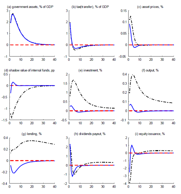
Figure 4 presents the economic effects of the two policies. The blue solid line shows the case of direct lending/asset purchase policy and black solid-dotted line the case of capital injection. In panel (a), one can see that the two policy experiments are calibrated such that the sizes of government balance sheet relative to aggregate output in the two cases are roughly the same: In both cases, the government balance sheet immediately jumps up to 2 percent level in the first period, and continues to rise to reach the peak point of 2 3/4 percent in the third quarter. The government share starts running off very slowly thereafter and eventually reaches its steady state level, zero.

Panel (b) shows the implied (period-by-period) outlays for each policy. In both cases, the maximum outlay of about 2 percent of output is reached in the first period. While the government shares of assets continue to go up after the first intervention period, a large chunk of public resources is required only for the first period since the resources are being used to buy a stock of capital assets or intermediary shares. In fact, outlays drop significantly right after the first period, and only the first four periods are associated with positive outlays. Starting from the fifth period, both policies generate a substantial amount of net profits and allow the government to disburse large amounts of money to the households as transfer. The potential payback to the households may be underestimated in our exercises because we perform the experiments around the steady state while such policies are likely to be implemented during crises when prices of asset are unusually low, which may not be well captured by a local approximation.²⁰

In panel (c), one can see that the prices of capital assets immediately jump with the policies in both cases, although the peak size and the duration of price boost is slightly greater for capital injection policy. Given our choice for a relatively small adjustment friction in investment, the magnitude of asset prices responses are not big. Nevertheless, such an increase in the asset prices improves overall balance sheet conditions of the intermediaries in both cases. One can read this from the drop in the shadow value of internal funds, panel (d).

However, panel (d) reveals a very different picture about the efficacy of the two policies in generating desired stabilization effect: The drop in the shadow value, which is the best summary measure of the liquidity/balance sheet conditions in our framework, is almost five times greater for capital injection policy, suggesting that the capital injection policy may be much more powerful than the direct lending/asset purchase policy in handling liquidity/balance sheet crisis. Panel (e) and (f) confirm this: In terms of peak response, the capital injection policy induces 5 to 6 times greater impacts on aggregate investment and output. What explains this difference?

Panel (g) provides the answer: In contrast to capital injection policy, the direct lending/asset purchase policy suffers from a classic case of `crowding out' effect. To understand this point, it is useful to realize that the two policies act on asset markets differently. When the direct lending/asset purchase policy is executed, holding the market prices of assets constant, the policy shifts the supply of capital for private sector to the left, reducing the supply from $K_{t+1}$ to $(1-S_{t+1}^{S,G})K_{t+1}$ . As a consequence, asset prices go up while the private demand for assets decreases along the downward demand curve. While overall improvement in liquidity condition and business environment helps the demand recover, this is not enough to overcome the initial crowding out effect, as confirmed by the large decline in private lending (investment) shown in panel (g). This explains why the size of the stimulative effect dies out so quickly.

The capital injection policy works in a different way. It improves the liquidity/balance sheet conditions of the intermediaries, which increases the risk appetite for capital assets as suggested by the massive drop in the shadow value in panel (d), making both the prices and the quantities of asset expand in the same direction. Roughly speaking, the vertical distance between the responses of private lending in panel (g) explains a large chunk of the difference in the efficacy of two policies.

More fundamentally, by tying the cash injection to the amount of equity financing, the policy makes the firms reveal their liquidity conditions and allows the public resources to be directed to the right place - directly at the location where the problem originates. In contrast, the direct asset purchase policy strengthens the balance sheets condition of all intermediaries, not only the cash strapped institutions, and cannot prevent the ones with large amount of surplus cash flow from paying out the extra profits as dividends (and perhaps bonuses in reality).²¹ Note that while the sizes of dividend payouts are similar in both cases, the payouts in the case of asset purchase policy are less warranted from the perspective of a policy maker given the lackluster fundamental of the economy (see panel (h)). It is also notable that the asset purchase policy is less successful in reducing the amount of costly equity finance (hence less dependence on retained earning) because it is less effective in improving internal cash flow of intermediaries.

4.3 Transitional Dynamics to Higher Levels of Capitalization

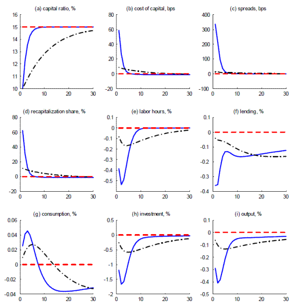
The current policy proposal from the Basel 3 process envisions a roughly 5 percentage point increase in the required ratio of common equity to risk-weighted assets (from 2 percent to 7 percent) or in the ratio of tier 1 capital to risk-weighted assets (from 4 to 8 percent). In the data, overall capital ratios have substantially exceeded these minima, both because regulators have defined well capitalized as some notable margin above the minimum and because market pressures have led financial institutions to maintain capital buffers. Consistent with various policy analyses, we assume that the increase in the regulatory minimum is passed through to overall capital ratios and consider an increase in the overall ratio of capital to assets from 10 percent to 15 percent.

We design two transition arrangements to compare two cases, fast vs slow transitions: one in which the capital ratio is raised by 5 percentage points approximately in 8 quarters and the other in which the capital ratio is raised by the same amount, but in 32 quarters. To achieve the transitional paths for the minimum capital ratio, we assume the following data generating process for the minimum capital ratio,

$\displaystyle \log m_{t}$	$\displaystyle =\log m_{t-1}+\delta_{t},$
$\displaystyle \delta_{t}$	$\displaystyle =\rho v_{t-1}+u_{t}.$

By setting an appropriate value $\rho$ , one can control how fast the capital ratio reaches a new long run value. In the case of fast transition, we set $\rho=0.5$ while we $\rho=0.85$ for the case of slow transition.

Figure 5 displays the two transitional paths for selected endogenous variables under the baseline calibration. Panel (a) shows the two transition arrangements for the permanent increase in regulatory capital ratio. In both cases, financial intermediaries face significant capital shortfalls, creating funding pressure, which leads to significantly higher costs of capital for the intermediaries as shown in panel (b). However, the slower transition is associated with a disproportionately milder rise in the cost of capital, roughly only 1/4 of increase in the cost of capital as compared with the case in the fast transition. As a consequence, the spillover effect on the general lending terms in other financial markets, shown in panel (c), is much more mitigated: while the fast transition result in a maximum 300 bps increase in credit spreads, the credit spreads in the case of slow transition are maximized at around 20 bps.

In panel (d), one can see why the slower transition is associated with smaller financial costs. The picture displays how much of the required increase in capital at each point in time is obtained by the costly equity issuance. In the faster transition case, the intermediaries have to tap equity market more intensively as the funding needs far outstrip the available cashflows. Panel (f) highlights the same point from a different angle: the faster transition is associated with much more aggressive contraction in lending. As both equity finance and decreasing lending are costly to the banks, intermediaries balance the two margins. The much higher funding costs, the loss of profitable lending opportunities, and further deterioration in cash flow owing to the ensuing overall economic downturn result in a massive drop in the price of intermediary shares in panel (e). In contrast, the slower transition allows the banks to earn their way out by relying more on the accumulation of retained earnings, allowing them to avoid the much more costly financing options and hence limiting the harmful effects on credit provision. Finally, as predicted by the effects on the credit spreads and lending, panel (e) $\sim$ (i) show that the faster implementation takes a much greater toll on economic activity: the declines in hours, lending, investment and output are about 2 to 3 times greater for the case of faster transition.

5 Conclusion

In this research, we consider a tractable macroeconomic model in which real investment is intermediated through institutions that commit financial resources amid idiosyncratic funding risk under a binding capital constraint. We show that the share of equity in the financing base of intermediaries is neutral in the long run, but not in the short run, and that financial frictions facing intermediaries imply a sizable equity premium for the aggregate economy. We then consider credit policies designed to address liquidity/balance sheet problems at intermediaries and show that a capital injection policy conditioned on voluntary recapitalization is relatively efficient because it does not suffer from a "crowding out" effect on private investment. With regard to long-run policies, we demonstrate that a transition to higher capital requirements can have sizable short-run effects on economic activity if not implemented carefully, and that a long transition period helps avoid such effects.

Bibliography

Admati, A. R., P. M. DeMarzo, M. F. Hellwig, and P. Pfleiderer (2010, September).

Fallacies, irrelevant facts, and myths in the discussion of capital regulation: Why bank equity is not expensive.
Research Papers, 2065, Stanford University, Graduate School of Business.

Adrian, T. and H. S. Shin, (2008).

Financial intermediary leverage and value at risk.
Staff Reports 338, Federal Reserve Bank of New York.

Adrian, T. and H. S. Shin, (2010).

Financial intermediaries and monetary economics.
Volume 3 of Handbook of Monetary Economics, pp. 601 - 650. Elsevier.

BIS (2010a).

Assessing the macroeconomic impact of the transition to stronger capital and liquidity requirements.
Interim report of the macroeconomic assessment group, Basel Committee on Banking Supervision, Basel, Switzerland.

BIS (2010b).

An assessment of the long-term economic impact of stronger capital and liquidity requirements.
Technical report, Basel Committee on Banking Supervision, Basel, Switzerland.

Boivin, J., M. T. Kiley, and F. S. Mishkin, (2010).

How has the monetary transmission mechanism evolved over time?
Volume 3 of Handbook of Monetary Economics, pp. 369 - 422. Elsevier.

Bolton, P. and X. Freixas, (2000).

Equity, bonds, and bank debt: Capital structure and financial market equilibrium under assymetric information.
The Journal of Political Economy 108(2), pp. 324-351.

Brunnermeier, M. K. and L. H. Pedersen, (2009).

Market Liquidity and Funding Liquidity.
Review of Financial Studies 22(6), 2201-2238.

CBO, (2011).

Report on the troubled asset relief program.
Pub. No. 4253, Congressional Budget Office.

Christiano, L., R. Motto, and M. Rostagno, (2003).

The great depression and the friedman-schwartz hypothesis.
Journal of Money, Credit and Banking 35(6), 1119-1197.

Cooley, T. F. and V. Quadrini, (2001).

Financial markets and firm dynamics.
The American Economic Review 91(5), pp. 1286-1310.

Demirguc, A., L. Laeven, and R. Levine (2003, April).

The impact of bank regulations, concentration, and institutions on bank margins.
Policy Research Working Paper Series, 3030, The World Bank.

Diamond, D. W. and R. G. Rajan, (2000).

A theory of bank capital.
The Journal of Finance 55(6), pp. 2431-2465.

Gertler, M. and N. Kiyotaki, (2010).

Financial intermediation and credit policy in business cycle analysis.
Volume 3 of Handbook of Monetary Economics, pp. 547 - 599. Elsevier.

Gomes, J. F., (2001).

Financing investment.
The American Economic Review 91(5), pp. 1263-1285.

Hanson, S. G., A. K. Kashyap, and J. C. Stein, (2011).

A macroprudential approach to financial regulation.
Journal of Economic Perspectives 25(1), 3-28.

He, Z. and A. Krishnamurthy (2008, December).

Intermediary asset pricing.
NBER Working Papers, 14517, National Bureau of Economic Research, Inc.

Hennessy, C. A. and T. M. Whited, (2007).

How costly is external financing? evidence from a structural estimation.
The Journal of Finance 62(4), pp. 1705-1745.

Holmström, B. and J. Tirole, (2001).

Lapm: A liquidity-based asset pricing model.
The Journal of Finance 56(5), pp. 1837-1867.

Janicki, H. P. and E. S. Prescott, (2006).

Changes in the size distribution of u.s. banks: 1960-2005.
Economic Quarterly (Fall), 291-316.

Jermann, U. and V. Quadrini (2009, September).

Macroeconomic effects of financial shocks.
NBER Working Papers, 15338, National Bureau of Economic Research, Inc.

Johnson, N. L., S. Kotz, and N. Balakrishnan, (1994).

Continuous Univariate Distributions (2nd ed.), Volume 1.
Wiley.

Kiley, M. T. and J. W. Sim, (2011).

Financial capital and the macroeconomy: A quantitative framework.
Finance and Economics Discussion Series 2011-27, Board of Governors of the Federal Reserve System (U.S.).

Myers, S. C. and N. S. Majluf, (1984).

Corporate financing and investment decisions when firms have information that investors do not have.
Journal of Financial Economics 13(2), 187 - 221.

Ross, S. A., (1977).

The determination of financial structure: The incentive-signalling approach.
The Bell Journal of Economics 8(1), pp. 23-40.

Saunders, A. and L. Schumacher, (2000).

The determinants of bank interest rate margins: an international study.
Journal of International Money and Finance 19(6), 813 - 832.

Shleifer, A. and R. W. Vishny, (1997).

The limits of arbitrage.
The Journal of Finance 52(1), pp. 35-55.

Sidrauski, M., (1967).

Inflation and economic growth.
The Journal of Political Economy 75(6), 796-810.

Smets, F. and R. Wouters, (2007).

Shocks and frictions in us business cycles: A bayesian dsge approach.
The American Economic Review 97(3), 586-606.

Van den Heuvel, S. J., (2008).

The welfare cost of bank capital requirements.
Journal of Monetary Economics 55(2), 298 - 320.

Wen, Y., (2009).

An analytical approach to buffer-stock saving.
Technical report.

Figure 1: Uncertainty, Cost of Equity Issuance and Return Premium Figure 1. Uncertainty, Cost of Equity Issuance and Return Premium. Link to accessible version follows.

Accessible Version

Figure 2: Long-run Neutrality of Capital Constraint: vs . Figure 2. Link to accessible version follows.

Accessible Version

Figure 3:Impact of Intermediation Shock in Model and Data (from identified VAR, see Kiley and Sim (2011)). Figure 3. Impact of Intermediation Shock in Model and Data. Link to accessible version follows.

Accessible Version

Figure 4: Efficacy of Policy Intervention: Asset Purchase (blue solid) vs Capital Injection (black dash-dot). Figure 4. Efficacy of Policy Intervention: Asset Purchase (blue solid) vs Capital Injection (black dash-dot). Link to accessible version follows.

Accessible Version

Figure 5: Transitional Dynamics of Capital Standards: Fast (blue solid) vs Slow (black dash-dot) Transition Arrangement. Figure 5. Transitional Dynamics of Capital Standards: Fast (blue solid) vs Slow (black dash-dot) Transition Arrangement. Link to accessible version follows.

Accessible Version

Footnotes

* We would like to thank seminar participants at the 2011 ASSA meetings, the Board of Governors of the Federal Reserve System, the Bank of Canada, and the Bank of Japan for comments on an earlier draft (circulated under the title "The Dynamic Effects of Bank Capital in General Equilibrium"). The views expressed herein are those of the authors, and do not reflect the views of the Federal Reserve Board or its staff. Return to Text

1. For a discussion of capital requirements, see BIS (2010a) and BIS (2010b). For a recent summary of the Troubled Asset Relief Program (TARP), which included measures to stabilize the balance sheet position of financial intermediaries, see CBO (2011). Return to Text

2. The intermediary specific pricing kernel in our framework provides a structural justification of the time-varying discount factor of Jermann and Quadrini (2009), who derive a superficially-similar pricing kernel from a reduced-form quadratic adjustment cost for dividends. Other work developing intermediary-specific discount factors includes He and Krishnamurthy (2008), who derive their intermediary-specific pricing kernel by assuming risk aversion for financial intermediaries. Return to Text

3. He and Krishnamurthy (2008) also suggest that capital injections are more effective than asset purchases, but their focus is on the asset market recovery. Our framework provides a more comprehensive assessment of impacts of the stabilization policies on employment, investment and output in a production-based business-cycle framework. Return to Text

4. In broad terms, the return structure of our intermediaries share aspects of those analyzed by Gertler and Kiyotaki (2010). Return to Text

5. Janicki and Prescott (2006) show that a lognormal distribution is a good approximation of the size distribution of the banks in U.S. In Kiley and Sim (2011), we consider a time-varying uncertainty process, where the parameter $\sigma$ follows a Markov process, and explore the implication of an increase in uncertainty for the cost of capital and economic activity. Return to Text

6. Such a constraint also can exist as a consequence of imperfect contract enforceability as in Gertler and Kiyotaki (2010) . As will be made clear below, the risk-neutrality of intermediary, the linearity of investment technology and the linearity of equity floating cost imply that the intermediary problem is linearly homogeneous such that the intermediary value function can be expressed as $V_{t}=\nu_{t}Q_{t-1} K_{t}-\varsigma_{t}B_{t}$ as in Gertler and Kiyotaki (2010) despite the difference in capital structure choices of the two approaches . It is then straightforward to derive the capital constraint by requiring that the value of firm should be greater than a lower bound for the firm value, $\bar{V}_{t}$ . One structural interpretation of the lower bound could be that of Gertler and Kiyotaki (2010): assuming that $\xi_{t}$ portion of balance sheet asset is divertable, one could derive the constraint from an incentive compatibility, i.e., $\nu_{t}Q_{t-1}K_{t}-\varsigma_{t}B_{t}\geq\xi_{t} Q_{t-1}K_{t}$ . In this case, the minimum capital ratio can be seen as $m_{t}=1-(\nu_{t}-\xi_{t})/\varsigma_{t}$ . Return to Text

7. A similar timing convention has been used by Wen (2009) in the context of buffer stock saving of risk-averse households and by Gertler and Kiyotaki (2010) in the context of interbank market borrowing decision of risk neutral banks. Note that interbank borrowing, a possibility from which we abstract, does not ameliorate the potential funding distortions under realistic assumptions. In particular, borrowing more through the interbank market to cope with cash flow shortfalls simply worsens any funding shortfall because it increases leverage. An efficient secondary market for balance sheet assets could help in this situation. However, it is natural to assume that the same information problem that makes equity finance costly also makes interbank transfer of balance sheet assets difficult (as was apparent in the financial crisis of 2008, where secondary markets for bank loans became severely distressed). Return to Text

8. In reality, the cost of issuing equity could stem from many sources. For example, outsiders who invest in new shares of the intermediary may not be able to distinguish a negative income shock from diversion or inefficiency of management. In such an environment, outsiders need to investigate the balance sheet of the intermediary before they invest to verify that the intermediary complies with the rule of truthful reporting. Furthermore, as shown by Ross (1977) and Myers and Majluf (1984), outsiders, not knowing the true investment opportunities of the intermediary, require initial discounts to protect themselves from "lemons". This type of friction is evident in market data, where, for example, equity issuance costs take the form of underwriting fees for investment banks and initial discounts of seasoned equity offerings (SEOs). Return to Text

9. Gomes (2001) points out that the per unit cost of equity issuance is either constant or declining, exhibiting an increasing returns to scale. An alternative approach considered in Jermann and Quadrini (2009) assumes a quadratic adjustment cost in dividend payouts/equity issuance. Such an assumption is motivated by empirical evidence that dividend payouts are smooth. In contrast to dividend payouts, equity financing and/or share repurchases are better described as lumpy, discrete event. In reality, modeling the mix of smooth dividend streams and lumpy equity issuance/share repurchases jointly would require considering a very complicated corporate financing problem, which lies well outside our interest in focusing on key factors driving the links between bank capitalization and real economic activity. Return to Text

10. There are other ways to ensure a binding capital constraint. For example, one can assume that the intermediary is impatient or subject to a constant death probability. Second, one can introduce a tax shield. Return to Text

11. See Johnson et al. (1994). Return to Text

12. The following property of lognormal distribution is used to derive the expression in the main text (see Johnson et al. (1994) ):

$\displaystyle \int_{\epsilon\geq\epsilon_{t}^{\ast}}\epsilon f(\epsilon\vert\sigma )d\epsilon=[1-\Phi(s_{t}^{\ast}-\sigma)]\int_{0}^{\infty}\epsilon f(\epsilon\vert\sigma)d\epsilon,$

where $f(\cdot\vert\sigma_{t})$ is the pdf of the lognormal distribution conditioned upon the parameter $\sigma$ and $s_{t}^{\ast}$ is defined as (11). Return to Text

13. We do not consider a short sale policy of the government. Hence, $0\leq S_{t}^{G} (i)\leq1$ . Return to Text

14. Recent application also can be found in Van den Heuvel (2008). Return to Text

15. Note that in the frictionless economy, the marginal cost and the average cost of capital identical since the shadow value of internal funds is always equal to one. Return to Text

16. The general equilibrium effect in this analysis is reminiscent of, but economically quite different from, the mechanism underlying the celebrated Miller-Modigliani theorem, where a shift in the mix of debt and equity changes the risk associated with each type of liability. The intermediary deposits are default risk-free in our analysis. Return to Text

17. The loci in the picture show the values of $R^{B}$ that satisfy the equilibrium conditions for 3,000 points $R^{F}$ between 1.040 and 1.065. We solve for these values using a nonlinear numerical root finder. Return to Text

18. Kiley and Sim (2011) report more details and robustness checks. Return to Text

19. To model time-varying uncertainty, we assume the following process:

$\displaystyle \log\sigma_{t}=(1-\rho_{\sigma})\log\bar{\sigma}+\rho_{\sigma}\log\sigma _{t-1}+u_{t}$ , $\displaystyle u_{t}\sim$ iid $\displaystyle N(0,\Sigma^{2}).$

(34)

We set $\rho_{\sigma}=0.85$ ; Kiley and Sim (2011) present more details Return to Text

20. The fact that the initial outlays of such policies overstate the long-run budget costs because of subsequent revenues from the purchased assets has been discussed in related policy discussions, e.g., CBO (2011). Return to Text

21. This last aspect was not highlighted by Gertler and Kiyotaki (2010) because the intermediaries in their framework never pay out dividends (their problem is a terminal value maximization). Return to Text

^♣ This version is optimized for use by screen readers. Descriptions for all mathematical expressions are provided in LaTex format. A printable pdf version is available. Return to Text

$\displaystyle \mathbb{E}_{t}^{i}[\lambda_{t}(i)]$	$\displaystyle =\mu_{t}(i)(1-m_{t})$	(6)
	$\displaystyle +$ $\displaystyle \beta\mathbb{E}_{t}\left[ \frac{\Lambda_{t+1}}{\Lambda_{t}} \mathbb{E}_{t+1}^{i}[\lambda_{t+1}(i)\epsilon_{t+1}(i)]\frac{R_{t+1}^{F}}{ \Pi_{t+1}}\right]$

$\displaystyle P_{t}^{S}(i)$	$\displaystyle =\beta\mathbb{E}_{t}\left\{ \frac{\Lambda_{t+1}}{\Lambda_{t} }\mathbb{E}_{t+1}^{i}[\max\{D_{t+1}(i),0\}\right.$	(25)
	$\displaystyle \left. \underset{}{\overset{}{+[1-(1-S_{t+2}^{G})\bar{\varphi} ]\min\{D_{t+1}(i),0\}+P_{t+1}^{S}(i)]}}\right\}$

Financial Capital and the Macroeconomy: Policy Considerations*

Financial Capital and the Macroeconomy:
Policy Considerations*