
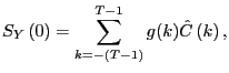
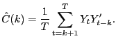
Board of Governors of the Federal Reserve System
International Finance Discussion Papers
Number 866, August 2006-Screen Reader Version*
Assessing Structural VARs*
NOTE: International Finance Discussion Papers are preliminary materials circulated to stimulate discussion and critical comment. References in publications to International Finance Discussion Papers (other than an acknowledgment that the writer has had access to unpublished material) should be cleared with the author or authors. Recent IFDPs are available on the Web at http://www.federalreserve.gov/pubs/ifdp/. This paper can be downloaded without charge from the Social Science Research Network electronic library at http://www.ssrn.com/.
Abstract:
This paper analyzes the quality of VAR-based procedures for estimating the response of the economy to a shock. We focus on two key issues. First, do VAR-based confidence intervals accurately reflect the actual degree of sampling uncertainty associated with impulse response functions? Second, what is the size of bias relative to confidence intervals, and how do coverage rates of confidence intervals compare with their nominal size? We address these questions using data generated from a series of estimated dynamic, stochastic general equilibrium models. We organize most of our analysis around a particular question that has attracted a great deal of attention in the literature: How do hours worked respond to an identified shock? In all of our examples, as long as the variance in hours worked due to a given shock is above the remarkably low number of 1 percent, structural VARs perform well. This finding is true regardless of whether identification is based on short-run or long-run restrictions. Confidence intervals are wider in the case of long-run restrictions. Even so, long-run identified VARs can be useful for discriminating among competing economic models.
Keywords: Vector autoregression, dynamic stochastic general equilibrium model, confidence intervals, impulse response functions, identification, long run restrictions, specification error, sampling
JEL Classification: C1
1 Introduction
Sims's seminal paper Macroeconomics and Reality (1980) argued that procedures based on vector autoregression (VAR) would be useful to macroeconomists interested in constructing and evaluating economic models. Given a minimal set of identifying assumptions, structural VARs allow one to estimate the dynamic effects of economic shocks. The estimated impulse response functions provide a natural way to choose the parameters of a structural model and to assess the empirical plausibility of alternative models.1
To be useful in practice, VAR-based procedures must have good sampling properties. In particular, they should accurately characterize the amount of information in the data about the effects of a shock to the economy. Also, they should accurately uncover the information that is there.
These considerations lead us to investigate two key issues. First, do VAR-based confidence intervals accurately reflect the actual degree of sampling uncertainty associated with impulse response functions? Second, what is the size of bias relative to confidence intervals, and how do coverage rates of confidence intervals compare with their nominal size?
We address these questions using data generated from a series of estimated dynamic, stochastic general equilibrium (DSGE) models. We consider real business cycle (RBC) models and the model in Altig, Christiano, Eichenbaum, and Linde (2005) (hereafter, ACEL) that embodies real and nominal frictions. We organize most of our analysis around a particular question that has attracted a great deal of attention in the literature: How do hours worked respond to an identified shock? In the case of the RBC model, we consider a neutral shock to technology. In the ACEL model, we consider two types of technology shocks as well as a monetary policy shock.
We focus our analysis on an unavoidable specification error that occurs when the data generating process is a DSGE model and the econometrician uses a VAR. In this case the true VAR is infinite ordered, but the econometrician must use a VAR with a finite number of lags.
We find that as long as the variance in hours worked due to a given shock is above the remarkably low number of 1 percent, VAR-based methods for recovering the response of hours to that shock have good sampling properties. Technology shocks account for a much larger fraction of the variance of hours worked in the ACEL model than in any of our estimated RBC models. Not surprisingly, inference about the effects of a technology shock on hours worked is much sharper when the ACEL model is the data generating mechanism.
Taken as a whole, our results support the view that structural VARs are a useful guide to constructing and evaluating DSGE models. Of course, as with any econometric procedure it is possible to find examples in which VAR-based procedures do not do well. Indeed, we present such an example based on an RBC model in which technology shocks account for less than 1 percent of the variance in hours worked. In this example, VAR-based methods work poorly in the sense that bias exceeds sampling uncertainty. Although instructive, the example is based on a model that fits the data poorly and so is unlikely to be of practical importance.
Having good sampling properties does not mean that structural VARs always deliver small confidence intervals. Of course, it would be a Pyrrhic victory for structural VARs if the best one could say about them is that sampling uncertainty is always large and the econometrician will always know it. Fortunately, this is not the case. We describe examples in which structural VARs are useful for discriminating between competing economic models.
Researchers use two types of identifying restrictions in structural VARs. Blanchard and Quah (1989), Gali (1999), and others exploit the implications that many models have for the long-run effects of shocks.2 Other authors exploit short-run restrictions.3 It is useful to distinguish between these two types of identifying restrictions to summarize our results.
We find that structural VARs perform remarkably well when identification is based on short-run restrictions. For all the specifications that we consider, the sampling properties of impulse response estimators are good and sampling uncertainty is small. This good performance obtains even when technology shocks account for as little as 0.5 percent of the variance in hours. Our results are comforting for the vast literature that has exploited short-run identification schemes to identify the dynamic effects of shocks to the economy. Of course, one can question the particular short-run identifying assumptions used in any given analysis. However, our results strongly support the view that if the relevant short-run assumptions are satisfied in the data generating process, then standard structural VAR procedures reliably uncover and identify the dynamic effects of shocks to the economy.
The main distinction between our short and long-run results is that the sampling uncertainty associated with estimated impulse response functions is substantially larger in the long-run case. In addition, we find some evidence of bias when the fraction of the variance in hours worked that is accounted for by technology shocks is very small. However, this bias is not large relative to sampling uncertainty as long as technology shocks account for at least 1 percent of the variance of hours worked. Still, the reason for this bias is interesting. We document that, when substantial bias exists, it stems from the fact that with long-run restrictions one requires an estimate of the sum of the VAR coefficients. The specification error involved in using a finite-lag VAR is the reason that in some of our examples, the sum of VAR coefficients is difficult to estimate accurately. This difficulty also explains why sampling uncertainty with long-run restrictions tends to be large.
The preceding observations led us to develop an alternative to the standard VAR-based estimator of impulse response functions. The only place the sum of the VAR coefficients appears in the standard strategy is in the computation of the zero-frequency spectral density of the data. Our alternative estimator avoids using the sum of the VAR coefficients by working with a nonparametric estimator of this spectral density. We find that in cases when the standard VAR procedure entails some bias, our adjustment virtually eliminates the bias.
Our results are related to a literature that questions the ability of long-run identified VARs to reliably estimate the dynamic response of macroeconomic variables to structural shocks. Perhaps the first critique of this sort was provided by Sims (1972). Although his paper was written before the advent of VARs, it articulates why estimates of the sum of regression coefficients may be distorted when there is specification error. Faust and Leeper (1997) and Pagan and Robertson (1998) make an important related critique of identification strategies based on long-run restrictions. More recently Erceg, Guerrieri, and Gust (2005) and Chari, Kehoe, and McGrattan (2005b) (henceforth CKM) also examine the reliability of VAR-based inference using long-run identifying restrictions.4Our conclusions regarding the value of identified VARs differ sharply from those recently reached by CKM. One parameterization of the RBC model that we consider is identical to the one considered by CKM. This parameterization is included for pedagogical purposes only, as it is overwhelmingly rejected by the data.
The remainder of the paper is organized as follows. Section 2 presents the versions of the RBC models that we use in our analysis. Section 3 discusses our results for standard VAR-based estimators of impulse response functions. Section 4 analyzes the differences between short and long-run restrictions. Section 5 discusses the relation between our work and the recent critique of VARs offered by CKM. Section 6 summarizes the ACEL model and reports its implications for VARs. Section 7 contains concluding comments.
2 A Simple RBC Model
In this section, we display the RBC model that serves as one of the data generating processes in our analysis. In this model the only shock that affects labor productivity in the long-run is a shock to technology. This property lies at the core of the identification strategy used by King, et al (1991), Gali (1999) and other researchers to identify the effects of a shock to technology. We also consider a variant of the model which rationalizes short run restrictions as a strategy for identifying a technology shock. In this variant, agents choose hours worked before the technology shock is realized. We describe the conventional VAR-based strategies for estimating the dynamic effect on hours worked of a shock to technology. Finally, we discuss parameterizations of the RBC model that we use in our experiments.
2.1 The Model
The representative agent maximizes expected utility over per
capita consumption, ![]() and per capita hours worked,
and per capita hours worked, ![]()
![$\displaystyle E_{0}\sum_{t=0}^{\infty}\left( \beta\left( 1+\gamma\right) \right... ... \log c_{t}+\psi\frac{\left( 1-l_{t}\right) ^{1-\sigma}-1}{1-\sigma }\right] , $](img4.gif)
The representative competitive firm's production function is:
where
Finally, the resource constraint is:
We consider two versions of the model, differentiated according
to timing assumptions. In the standard
or nonrecursive version, all time
![]() decisions are taken
after the realization of the time
decisions are taken
after the realization of the time ![]() shocks. This is the conventional assumption in the
RBC literature. In the recursive
version of the model the timing assumptions are as follows.
First,
shocks. This is the conventional assumption in the
RBC literature. In the recursive
version of the model the timing assumptions are as follows.
First,
![]() is observed,
and then labor decisions are made. Second, the other shocks are
realized and agents make their investment and consumption
decisions.
is observed,
and then labor decisions are made. Second, the other shocks are
realized and agents make their investment and consumption
decisions.
2.2 Relation of the RBC Model to VARs
We now discuss the relation between the RBC model and a VAR. Specifically, we establish conditions under which the reduced form of the RBC model is a VAR with disturbances that are linear combinations of the economic shocks. Our exposition is a simplified version of the discussion in Fernandez-Villaverde, Rubio-Ramirez, and Sargent (2005) (see especially their section III). We include this discussion because it frames many of the issues that we address. Our discussion applies to both the standard and the recursive versions of the model.
We begin by showing how to put the reduced form of the RBC model
into a state-space, observer form. Throughout, we analyze the
log-linear approximations to model solutions. Suppose the variables
of interest in the RBC model are denoted by ![]() Let
Let ![]() denote the vector of exogenous
economic shocks and let
denote the vector of exogenous
economic shocks and let
![]() denote the
percent deviation from steady state of the capital stock, after
scaling by
denote the
percent deviation from steady state of the capital stock, after
scaling by ![]() 5 The approximate solution for
5 The approximate solution for
![]() is given by:
is given by:
where
Also,
where
The `state' of the system is composed of the variables on the right side of (2):
![\begin{displaymath} \xi_{t}=\left( \begin{array}[c]{c} \hat{k}_{t}\ \hat{k}_{t-1}\ s_{t}\ s_{t-1} \end{array}\right) . \end{displaymath}](img53.gif)
where
Here,
We now use (5) and (6) to establish conditions under which the reduced
form representation for ![]() implied by the RBC model is a VAR with
disturbances that are linear combinations of the economic shocks.
In this discussion, we set
implied by the RBC model is a VAR with
disturbances that are linear combinations of the economic shocks.
In this discussion, we set ![]() so that
so that
![]() In
addition, we assume that the number of elements in
In
addition, we assume that the number of elements in
![]() coincides with the number of elements in
coincides with the number of elements in ![]()
We begin by substituting (5) into (6) to obtain:
Substituting (7) into (5), we obtain:
As long as the eigenvalues of
Using (9) to substitute out for
where
Expression (10) is an infinite-order VAR, because
Proposition 2.1. (Fernandez-Villaverde, Rubio-Ramirez, and Sargent) If C is invertible and the eigenvalues of M are less than unity in absolute value, then the RBC model implies:
![]() has the
infinite-order VAR representation in (10)
has the
infinite-order VAR representation in (10)
![]() The linear
one-step-ahead forecast error
The linear
one-step-ahead forecast error ![]() given past
given past ![]() 's is
's is ![]() , which is related to the economic disturbances
by (11)
, which is related to the economic disturbances
by (11)
![]() The
variance-covariance of
The
variance-covariance of ![]() is
is
![]()
![]() The sum of the
VAR lag matrices is given by:
The sum of the
VAR lag matrices is given by:
![$ B(1)\equiv\sum\limits_{j=1}^{\infty}B_{j}=HF\left[ I-M\right] ^{-1}DC^{-1} $](img11last.gif)
We will use the last of these results below.
Relation (10) indicates why researchers
interested in constructing DSGE models find it useful to analyze
VARs. At the same time, this relationship clarifies some of the
potential pitfalls in the use of VARs. First, in practice the
econometrician must work with finite lags. Second, the assumption
that ![]() is square and
invertible may not be satisfied. Whether
is square and
invertible may not be satisfied. Whether ![]() satisfies these conditions depends
on how
satisfies these conditions depends
on how ![]() is
defined. Third, significant measurement errors may exist. Fourth,
the matrix,
is
defined. Third, significant measurement errors may exist. Fourth,
the matrix, ![]() , may not
have eigenvalues inside the unit circle. In this case, the economic
shocks are not recoverable from the VAR disturbances.6 Implicitly, the econometrician who
works with VARs assumes that these pitfalls are not quantitatively
important.
, may not
have eigenvalues inside the unit circle. In this case, the economic
shocks are not recoverable from the VAR disturbances.6 Implicitly, the econometrician who
works with VARs assumes that these pitfalls are not quantitatively
important.
2.3 VARs in Practice and the RBC Model
We are interested in the use of VARs as a way to estimate the
response of ![]() to
economic shocks, i.e., elements of
to
economic shocks, i.e., elements of
![]() In
practice, macroeconomists use a version of (10)
with finite lags, say
In
practice, macroeconomists use a version of (10)
with finite lags, say ![]() A researcher can estimate
A researcher can estimate
![]() and
and
![]() To obtain the impulse
response functions, however, the researcher needs the
To obtain the impulse
response functions, however, the researcher needs the ![]() 's and the column of
's and the column of ![]() corresponding to the shock in
corresponding to the shock in
![]() that is
of interest. However, to compute the required column of
that is
of interest. However, to compute the required column of
![]() requires additional
identifying assumptions. In practice, two types of assumptions are
used. Short-run assumptions take the form of direct restrictions on
the matrix
requires additional
identifying assumptions. In practice, two types of assumptions are
used. Short-run assumptions take the form of direct restrictions on
the matrix ![]() . Long-run
assumptions place indirect restrictions on
. Long-run
assumptions place indirect restrictions on ![]() that stem from restrictions on the
long-run response of
that stem from restrictions on the
long-run response of ![]() to
a shock in an element of
to
a shock in an element of
![]() . In
this section we use our RBC model to discuss these two types of
assumptions and how they are imposed on VARs in practice.
. In
this section we use our RBC model to discuss these two types of
assumptions and how they are imposed on VARs in practice.
2.3.1 The Standard Version of the Model
The log-linearized equilibrium laws of motion for capital and hours in this model can be written as follows:
and
From (2.13) and (2.14), it is clear that all shocks have only a temporary effect on
In our linear approximation to the model solution
In practice, researchers impose the exclusion and sign
restrictions on a VAR to compute
![]() and
identify its dynamic effects on macroeconomic variables. Consider
the
and
identify its dynamic effects on macroeconomic variables. Consider
the ![]() vector,
vector,
![]() The VAR for
The VAR for
![]() is given by:
is given by:
![$\displaystyle =\left( \begin{array}[c]{c} \Delta\log a_{t}\\ \log l_{t}\\ x_{t} \end{array} \right) .$](img116.gif)
Here,
Without loss of generality, we assume that the first element in
where
The symmetric matrix, ![]() and the
and the ![]() 's can be
computed using ordinary least squares regressions. However, the
requirement that
's can be
computed using ordinary least squares regressions. However, the
requirement that
![]() is not
sufficient to determine a unique value of
is not
sufficient to determine a unique value of ![]() Adding the exclusion and sign
restrictions does uniquely determine
Adding the exclusion and sign
restrictions does uniquely determine ![]() Relation (2.18) implies
that these restrictions are:
Relation (2.18) implies
that these restrictions are:
![\begin{displaymath}\left[ I-B(1)\right] ^{-1}C=\left[ \begin{array}[c]{cc} \text... ...ine{0}\ \text{numbers} & \text{numbers} \end{array}\right] , \end{displaymath}](img132.gif)
The exclusion restriction requires that
![\begin{displaymath} D=\left[ \begin{array}[c]{cc} \underset{1\times1}{d_{11}} & ... ...\right) \times\left( N-1\right) }{D_{22}} \end{array}\right] , \end{displaymath}](img142.gif)
![\begin{displaymath} DD^{\prime}=\left[ \begin{array}[c]{cc} d_{11}^{2} & d_{11}D... ...eft( 0\right) & S_{Y}^{22}\left( 0\right) \end{array}\right] , \end{displaymath}](img143.gif)
![\begin{displaymath} S_{Y}\left( \omega\right) \equiv\left[ \begin{array}[c]{cc} ... ...a\right) & S_{Y}^{22}\left( \omega\right) \end{array}\right] . \end{displaymath}](img144.gif)
There are two solutions to (2.20). The sign restriction
selects one of the two solutions to (2.20). So, the first column of
We conclude that
2.3.2 The Recursive Version of the Model
In the recursive version of the model, the policy rule for labor
involves
![]() and
and
![]() because these variables help forecast
because these variables help forecast
![]() and
and
![]()
As in the standard model, the only shock that affects
Let
![]() and
and
![]() denote the population one-step-ahead forecast errors in
denote the population one-step-ahead forecast errors in
![]() and
and
![]() conditional on the information set,
conditional on the information set,
![]() The
recursive version of the model implies that
The
recursive version of the model implies that
Because we normalize the standard deviation of
In practice, we implement the previous procedure using the
one-step-ahead forecast errors generated from a VAR in which the
variables in ![]() are
ordered as follows:
are
ordered as follows:
![\begin{displaymath} Y_{t}=\left( \begin{array}[c]{c} \log l_{t}\ \Delta\log a_{t}\ x_{t} \end{array}\right) . \end{displaymath}](img174.gif)
![\begin{displaymath}u_{t}=\left( \begin{array}[c]{c} u_{t}^{l}\ u_{t}^{a}\ u_{t}^{x} \end{array}\right) . \end{displaymath}](img176.gif)
![\begin{displaymath} C_{2}=\left( \begin{array}[c]{c} \frac{cov(u^{l},\varepsilon... ...\left( u_{t}^{x},u_{t}^{l}\right) \right) \end{array}\right) . \end{displaymath}](img183.gif)
2.4 Parameterization of the Model
We consider different specifications of the RBC model that are distinguished by the parameterization of the laws of motion of the exogenous shocks. In all specifications we assume, as in CKM , that:
2.4.1 Our MLE Parameterizations
We estimate two versions of our model. In the two-shock maximum likelihood estimation (MLE)
specification we assume that
![]() so that
there are two shocks,
so that
there are two shocks,
![]() and
and
![]() We
estimate the parameters
We
estimate the parameters ![]() ,
,
![]() and
and
![]() by
maximizing the Gaussian likelihood function of the vector,
by
maximizing the Gaussian likelihood function of the vector,
![]() subject to (24 )
subject to (24 )![]() 9 Our results are given by:
9 Our results are given by:
The three-shock MLE specification
incorporates the investment tax shock,
![]() into the
model. We estimate the three-shock MLE version of the model by
maximizing the Gaussian likelihood function of the vector,
into the
model. We estimate the three-shock MLE version of the model by
maximizing the Gaussian likelihood function of the vector,
![]() , subject to the parameter values in (24)
, subject to the parameter values in (24)![]() The
results are:
The
results are:
The estimated values of
2.4.2CKM Parameterizations
The two-shock CKM specification has two shocks, ![]() and
and
![]() These
shocks have the following time series representations:
These
shocks have the following time series representations:
The three-shock CKM specification adds an investment shock,
As in our specifications, CKM obtain their parameter estimates
using maximum likelihood methods. However, their estimates are very
different from ours. For example, the variances of the shocks are
larger in the two-shock CKM specification than in our MLE
specification. Also, the ratio of
![]() to
to
![]() is
nearly three times larger in the two-shock CKM specification than
in our two-shock MLE specification. Section 5 below discusses
the reasons for these differences.
is
nearly three times larger in the two-shock CKM specification than
in our two-shock MLE specification. Section 5 below discusses
the reasons for these differences.
2.5 The Importance of Technology Shocks for Hours Worked
Table 1 reports the contribution, ![]() of technology shocks to three different
measures of the volatility in the log of hours worked: (i) the
variance of the log hours, (ii) the variance of HP-filtered, log
hours and (iii) the variance in the one-step-ahead forecast error
in log hours.11 With one
exception, we compute the analogous statistics for log output. The
exception is (i), for which we compute the contribution of
technology shocks to the variance of the growth rate of output.
of technology shocks to three different
measures of the volatility in the log of hours worked: (i) the
variance of the log hours, (ii) the variance of HP-filtered, log
hours and (iii) the variance in the one-step-ahead forecast error
in log hours.11 With one
exception, we compute the analogous statistics for log output. The
exception is (i), for which we compute the contribution of
technology shocks to the variance of the growth rate of output.
The key result in this table is that technology shocks account
for a very small fraction of the volatility in hours worked. When
![]() is measured
according to (i), it is always below 4 percent. When
is measured
according to (i), it is always below 4 percent. When ![]() is measured using (ii) or (iii)
it is always below 8 percent. For both (ii) and (iii), in the CKM
specifications,
is measured using (ii) or (iii)
it is always below 8 percent. For both (ii) and (iii), in the CKM
specifications, ![]() is below 2 percent.12
Consistent with the RBC literature, the table also shows that
technology accounts for a much larger movement in output.
is below 2 percent.12
Consistent with the RBC literature, the table also shows that
technology accounts for a much larger movement in output.
Figure 1 displays visually how unimportant technology shocks are
for hours worked. The top panel displays two sets of 180 artificial
observations on hours worked, simulated using the standard
two-shock MLE specification. The volatile time series shows how log
hours worked evolve in the presence of shocks to both ![]() and
and
![]() The other
time series shows how log hours worked evolve in response to just
the technology shock,
The other
time series shows how log hours worked evolve in response to just
the technology shock, ![]() The bottom panel is the analog of the top
figure when the data are generated using the standard two-shock CKM
specification.
The bottom panel is the analog of the top
figure when the data are generated using the standard two-shock CKM
specification.
3 Results Based on RBC Data Generating Mechanisms
In this section we analyze the properties of conventional VAR-based strategies for identifying the effects of a technology shock on hours worked. We focus on the bias properties of the impulse response estimator, and on standard procedures for estimating sampling uncertainty.
We use the RBC model parameterizations discussed in the previous
section as the data generating processes. For each
parameterization, we simulate 1,000 data sets of 180 observations
each. The shocks
![]() ,
,
![]() and possibly
and possibly
![]() are drawn from
are drawn from ![]() standard normal distributions. For each artificial data set, we
estimate a four-lag VAR. The average, across the 1,000 data sets,
of the estimated impulse response functions, allows us to assess
bias.
standard normal distributions. For each artificial data set, we
estimate a four-lag VAR. The average, across the 1,000 data sets,
of the estimated impulse response functions, allows us to assess
bias.
For each data set we also estimate two different confidence intervals: a percentile-based confidence interval and a standard-deviation based confidence interval.13 We construct the intervals using the following bootstrap procedure. Using random draws from the fitted VAR disturbances, we use the estimated four lag VAR to generate 200 synthetic data sets, each with 180 observations. For each of these 200 synthetic data sets we estimate a new VAR and impulse response function. For each artificial data set the percentile-based confidence interval is defined as the top 2.5 percent and bottom 2.5 percent of the estimated coefficients in the dynamic response functions. The standard-deviation-based confidence interval is defined as the estimated impulse response plus or minus two standard deviations where the standard deviations are calculated across the 200 simulated estimated coefficients in the dynamic response functions.
We assess the accuracy of the confidence interval estimators in two ways. First, we compute the coverage rate for each type of confidence interval. This rate is the fraction of times, across the 1,000 data sets simulated from the economic model, that the confidence interval contains the relevant true coefficient. If the confidence intervals were perfectly accurate, the coverage rate would be 95 percent. Second, we provide an indication of the actual degree of sampling uncertainty in the VAR-based impulse response functions. In particular, we report centered 95 percent probability intervals for each lag in our impulse response function estimators.14 If the confidence intervals were perfectly accurate, they should on average coincide with the boundary of the 95 percent probability interval.
When we generate data from the two-shock MLE and CKM
specifications, we set
![]()
![]() When we generate data from the three-shock MLE and CKM
specifications, we set
When we generate data from the three-shock MLE and CKM
specifications, we set
![]()
3.1 Short-Run Identification
Figure 2 reports results generated from four different
parameterizations of the recursive version of the RBC model. In
each panel, the solid line is the average estimated impulse
response function for the 1,000 data sets simulated using the
indicated economic model. For each model, the starred line is the
true impulse response function of hours worked. In each panel, the
gray area defines the centered ![]() percent probability interval for the estimated
impulse response functions. The stars with no line indicate the
average percentile-based confidence intervals across the 1,000 data
sets. The circles with no line indicate the average
standard-deviation-based confidence intervals.
percent probability interval for the estimated
impulse response functions. The stars with no line indicate the
average percentile-based confidence intervals across the 1,000 data
sets. The circles with no line indicate the average
standard-deviation-based confidence intervals.
Figures 3 and 4 graph the coverage rates for the percentile-based and standard-deviation-based confidence intervals. For each case we graph how often, across the 1,000 data sets simulated from the economic model, the econometrician's confidence interval contains the relevant coefficient of the true impulse response function.
The 1,1 panel in Figure 2 exhibits the properties of the VAR-based estimator of the response of hours to a technology shock when the data are generated by the two-shock MLE specification. The 2,1 panel corresponds to the case when the data generating process is the three-shock MLE specification.
The panels have two striking features. First, there is essentially no evidence of bias in the estimated impulse response functions. In all cases, the solid lines are very close to the starred lines. Second, an econometrician would not be misled in inference by using standard procedures for constructing confidence intervals. The circles and stars are close to the boundaries of the gray area. The 1,1 panels in Figures 3 and 4 indicate that the coverage rates are roughly 90 percent. So, with high probability, VAR-based confidence intervals include the true value of the impulse response coefficients.
The second column of Figure 2 reports the results when the data generating process is given by variants of the CKM specification. The 1,2 and 2,1 panels correspond to the two and three-shock CKM specification, respectively.
The second column of Figure 2 contains the same striking features as the first column. There is very little bias in the estimated impulse response functions. In addition, the average value of the econometrician's confidence interval coincides closely with the actual range of variation in the impulse response function (the gray area). Coverage rates, reported in the 1,2 panels of Figures 3 and 4, are roughly 90 percent. These rates are consistent with the view that VAR-based procedures lead to reliable inference.
A comparison of the gray areas across the first and second columns of Figure 2, clearly indicates that more sampling uncertainty occurs when the data are generated from the CKM specifications than when they are generated from the MLE specifications (the gray areas are wider). VAR-based confidence intervals detect this fact.
3.2 Long-run Identification
The first and second rows of column 1 in Figure 5 exhibit our results when the data are generated by the two- and three- shock MLE specifications. Once again there is virtually no bias in the estimated impulse response functions and inference is accurate. The coverage rates associated with the percentile-based confidence intervals are very close to 95 percent (see Figure 3). The coverage rates for the standard-deviation-based confidence intervals are somewhat lower, roughly 80 percent (see Figure 4). The difference in coverage rates can be seen in Figure 5, which shows that the stars are shifted down slightly relative to the circles. Still, the circles and stars are very good indicators of the boundaries of the gray area, although not quite as good as in the analog cases in Figure 2.
Comparing Figures 2 and 5, we see that Figure 5 reports more sampling uncertainty. That is, the gray areas are wider. Again, the crucial point is that the econometrician who computes standard confidence intervals would detect the increase in sampling uncertainty.
The third and fourth rows of column 1 in Figure 5 report results
for the two and three - shock CKM specifications. Consistent with
results reported in CKM, there is substantial bias in the estimated
dynamic response functions. For example, in the Two-shock CKM
specification, the contemporaneous response of hours worked to a
one-standard-deviation technology shock is ![]() percent, while the mean
estimated response is
percent, while the mean
estimated response is ![]() percent. This bias stands in contrast to our
other results.
percent. This bias stands in contrast to our
other results.
Is this bias big or problematic? In our view, bias cannot be evaluated without taking into account sampling uncertainty. Bias matters only to the extent that the econometrician is led to an incorrect inference. For example, suppose sampling uncertainty is large and the econometrician knows it. Then the econometrician would conclude that the data contain little information and, therefore, would not be misled. In this case, we say that bias is not large. In contrast, suppose sampling uncertainty is large, but the econometrician thinks it is small. Here, we would say bias is large.
We now turn to the sampling uncertainty in the CKM specifications. Figure 5 shows that the econometrician's average confidence interval is large relative to the bias. Interestingly, the percentile confidence intervals (stars) are shifted down slightly relative to the standard-deviation-based confidence intervals (circles). On average, the estimated impulse response function is not in the center of the percentile confidence interval. This phenomenon often occurs in practice.15 Recall that we estimate a four lag VAR in each of our 1,000 synthetic data sets. For the purposes of the bootstrap, each of these VARs is treated as a true data generating process. The asymmetric percentile confidence intervals show that when data are generated by these VARs, VAR-based estimators of the impulse response function have a downward bias.
Figure 3 reveals that for the two- and three-shock CKM specifications, percentile-based coverage rates are reasonably close to 95 percent. Figure 4 shows that the standard deviation based coverage rates are lower than the percentile-based coverage rates. However even these coverage rates are relatively high in that they exceed 70 percent.
In summary, the results for the MLE specification differ from those of the CKM specifications in two interesting ways. First, sampling uncertainty is much larger with the CKM specification. Second, the estimated responses are somewhat biased with the CKM specification. But the bias is small: It has no substantial effect on inference, at least as judged by coverage rates for the econometrician's confidence intervals.
3.3 Confidence Intervals in the RBC Examples and a Situation in Which VAR-Based Procedures Go Awry
Here we show that the more important technology shocks are in
the dynamics of hours worked, the easier it is for VARs to answer
the question, `how do hours worked respond to a technology shock'.
We demonstrate this by considering alternative values of the
innovation variance in the labor tax,
![]() and by
considering alternative values of
and by
considering alternative values of ![]() the utility parameter that controls the Frisch
elasticity of labor supply.
the utility parameter that controls the Frisch
elasticity of labor supply.
Consider Figure 6, which focuses on the long-run identification
schemes. The first and second columns report results for the
two-shock MLE and CKM specifications, respectively. For each
specification we redo our experiments, reducing
![]() by a half
and then by a quarter. Table 1 shows that the importance of
technology shocks rises as the standard deviation of the labor tax
shock falls. Figure 6 indicates that the magnitude of sampling
uncertainty and the size of confidence intervals fall as the
relative importance of labor tax shocks falls.16
by a half
and then by a quarter. Table 1 shows that the importance of
technology shocks rises as the standard deviation of the labor tax
shock falls. Figure 6 indicates that the magnitude of sampling
uncertainty and the size of confidence intervals fall as the
relative importance of labor tax shocks falls.16
Figure 7 presents the results of a different set of experiments
based on perturbations of the two-shock CKM specification. The 1,1
and 2,1 panels show what happens when we vary the value of
![]() , the parameter
that controls the Frisch labor supply elasticity. In the 1,1 panel
we set
, the parameter
that controls the Frisch labor supply elasticity. In the 1,1 panel
we set ![]() which corresponds to a Frisch elasticity of 0.63. In the 2,1 panel,
we set
which corresponds to a Frisch elasticity of 0.63. In the 2,1 panel,
we set ![]() which corresponds to a Frisch elasticity of infinity. As the Frisch
elasticity is increased, the fraction of the variance in hours
worked due to technology shocks decreases (see Table 1). The
magnitude of bias and the size of confidence intervals are larger
for the higher Frisch elasticity case. In both cases the bias is
still smaller than the sampling uncertainty.
which corresponds to a Frisch elasticity of infinity. As the Frisch
elasticity is increased, the fraction of the variance in hours
worked due to technology shocks decreases (see Table 1). The
magnitude of bias and the size of confidence intervals are larger
for the higher Frisch elasticity case. In both cases the bias is
still smaller than the sampling uncertainty.
We were determined to construct at least one example in which
the VAR-based estimator of impulse response functions have bad
properties, i.e., bias is larger than sampling uncertainty. We
display such an example in the 3,1 panel of Figure 7. The data
generating process is a version of the two-shock CKM model with an
infinite Frisch elasticity and double the standard deviation of the
labor tax rate. Table 1 indicates that with this specification,
technology shocks account for a trivial fraction of the variance in
hours worked. Of the three measures of ![]() two are
two are ![]() percent and the third is
percent and the third is
![]() percent . The 3,1
panel of Figure 7 shows that the VAR-based procedure now has very
bad properties: the true value of the impulse response function
lies outside the average value of both confidence intervals that we
consider. This example shows that constructing scenarios in which
VAR-based procedures go awry is certainly possible. However, this
example seems unlikely to be of practical significance given the
poor fit to the data of this version of the model.
percent . The 3,1
panel of Figure 7 shows that the VAR-based procedure now has very
bad properties: the true value of the impulse response function
lies outside the average value of both confidence intervals that we
consider. This example shows that constructing scenarios in which
VAR-based procedures go awry is certainly possible. However, this
example seems unlikely to be of practical significance given the
poor fit to the data of this version of the model.
3.4 Are Long-Run Identification Schemes Informative?
Up to now, we have focused on the RBC model as the data generating process. For empirically reasonable specifications of the RBC model, confidence intervals associated with long-run identification schemes are large. One might be tempted to conclude that VAR-based long-run identification schemes are uninformative. Specifically, are the confidence intervals so large that we can never discriminate between competing economic models? Erceg, Guerrieri, and Gust (2005) show that the answer to this question is `no'. They consider an RBC model similar to the one discussed above and a version of the sticky wage-price model developed by Christiano, Eichenbaum, and Evans (2005) in which hours worked fall after a positive technology shock. They then conduct a series of experiments to assess the ability of a long-run identified structural VAR to discriminate between the two models on the basis of the response of hours worked to a technology shock.
Using estimated versions of each of the economic models as a data generating process, they generate 10,000 synthetic data sets each with 180 observations. They then estimate a four-variable structural VAR on each synthetic data set and compute the dynamic response of hours worked to a technology shock using long-run identification. Erceg, Guerrieri, and Gust (2005) report that the probability of finding an initial decline in hours that persists for two quarters is much higher in the model with nominal rigidities than in the RBC model (93 percent versus 26 percent). So, if these are the only two models contemplated by the researcher, an empirical finding that hours worked decline after a positive innovation to technology will constitute compelling evidence in favor of the sticky wage-price model.
Erceg, Guerrieri, and Gust (2005) also report that the probability of finding an initial rise in hours that persists for two quarters is much higher in the RBC model than in the sticky wage-price model (71 percent versus 1 percent). So, an empirical finding that hours worked rises after a positive innovation to technology would constitute compelling evidence in favor of the RBC model versus the sticky wage-price alternative.
4 Contrasting Short- and Long- Run Restrictions
The previous section demonstrates that, in the examples we
considered, when VARs are identified using short-run restrictions,
the conventional estimator of impulse response functions is
remarkably accurate. In contrast, for some parameterizations of the
data generating process, the conventional estimator of impulse
response functions based on long-run identifying restrictions can
exhibit noticeable bias. In this section we argue that the key
difference between the two identification strategies is that the
long-run strategy requires an estimate of the sum of the VAR
coefficients,
![]() This object is notoriously difficult to estimate accurately (see
Sims, 1972).
This object is notoriously difficult to estimate accurately (see
Sims, 1972).
We consider a simple analytic expression related to one in Sims
(1972). Our expression shows what an econometrician who fits a
misspecified, fixed-lag, finite-order VAR would find in population.
Let
![]() and
and ![]() denote the parameters of the
denote the parameters of the
![]() th-order VAR fit by
the econometrician. Then:
th-order VAR fit by
the econometrician. Then:
![$\displaystyle \hat{V}=V+\min_{\hat{B}_{1},...,\hat{B}_{q}}\frac{1}{2\pi}\int_{-... ... e^{i\omega}\right) -\hat{B}\left( e^{i\omega}\right) \right] ^{\prime}d\omega,$](img247.gif)
where
Here,
To understand the implications of (26) for
our analysis, it is useful to write in lag-operator form the
estimated dynamic response of ![]() to a shock in the first element of
to a shock in the first element of
![]()
where the
![$\displaystyle \theta_{k}=\frac{1}{2\pi}\int_{-\pi}^{\pi}\left[ I-\hat{B}\left( e^{-i\omega}\right) e^{-i\omega}\right] ^{-1}e^{k\omega i}d\omega.$](img276.gif)
In the case of long-run identification, the vector
We use (26) to understand why estimation
based on short-run and long-run identification can produce
different results. According to (27), impulse
response functions can be decomposed into two parts, the impact
effect of the shocks, summarized by
![]() and the
dynamic part summarized in the term in square brackets. We argue
that when a bias arises with long-run restrictions, it is because
of difficulties in estimating
and the
dynamic part summarized in the term in square brackets. We argue
that when a bias arises with long-run restrictions, it is because
of difficulties in estimating ![]() These difficulties do not arise with short-run
restrictions.
These difficulties do not arise with short-run
restrictions.
In the short-run identification case,
![]() is a
function of
is a
function of ![]() only.
Across a variety of numerical examples, we find that
only.
Across a variety of numerical examples, we find that ![]() is very close to
is very close to ![]() 21 This result is not surprising because
(26) indicates that the entire objective of
estimation is to minimize the distance between
21 This result is not surprising because
(26) indicates that the entire objective of
estimation is to minimize the distance between ![]() and
and ![]() In the long-run identification
case,
In the long-run identification
case,
![]() depends
not only on
depends
not only on ![]() but
also on
but
also on
![]() A problem is that the
criterion does not assign much weight to setting
A problem is that the
criterion does not assign much weight to setting
![]() unless
unless
![]() happens to be relatively
large in a neighborhood of
happens to be relatively
large in a neighborhood of ![]() But, a large value of
But, a large value of
![]() is not something one can rely on.22 When
is not something one can rely on.22 When
![]() is relatively small, attempts to match
is relatively small, attempts to match
![]() with
with
![]() at other frequencies can
induce large errors in
at other frequencies can
induce large errors in
![]()
The previous argument about the difficulty of estimating
![]() in the long-run
identification case does not apply to the
in the long-run
identification case does not apply to the
![]() s
s![]() According to (28)
According to (28)
![]() is a
function of
is a
function of
![]() over the whole
range of
over the whole
range of ![]() 's, not
just one specific frequency.
's, not
just one specific frequency.
We now present a numerical example, which illustrates Proposition 1 as well as some of the observations we have made in discussing (26). Our numerical example focuses on population results. Therefore, it provides only an indication of what happens in small samples.
To understand what happens in small samples, we consider four
additional numerical examples. First, we show that when the
econometrician uses the true value of
![]() , the
bias and much of the sampling uncertainty associated with the
Two-shock CKM specification disappears. Second, we demonstrate that
bias problems essentially disappear when we use an alternative to
the standard zero-frequency spectral density estimator used in the
VAR literature. Third, we show that the problems are attenuated
when the preference shock is more persistent. Fourth, we consider
the recursive version of the two-shock CKM specification in which
the effect of technology shocks can be estimated using either
short- or long-run restrictions.
, the
bias and much of the sampling uncertainty associated with the
Two-shock CKM specification disappears. Second, we demonstrate that
bias problems essentially disappear when we use an alternative to
the standard zero-frequency spectral density estimator used in the
VAR literature. Third, we show that the problems are attenuated
when the preference shock is more persistent. Fourth, we consider
the recursive version of the two-shock CKM specification in which
the effect of technology shocks can be estimated using either
short- or long-run restrictions.
Table 2 reports various properties of the two-shock CKM
specification. The first six ![]() 's in the infinite-order VAR, computed using
(12), are reported in Panel A. These
's in the infinite-order VAR, computed using
(12), are reported in Panel A. These
![]() 's eventually
converge to zero, however they do so slowly. The speed of
convergence is governed by the size of the maximal eigenvalue of
the matrix
's eventually
converge to zero, however they do so slowly. The speed of
convergence is governed by the size of the maximal eigenvalue of
the matrix ![]() in (8), which is 0.957. Panel B displays the
in (8), which is 0.957. Panel B displays the
![]() 's that
solve (26) with
's that
solve (26) with ![]() Informally, the
Informally, the
![]() 's look
similar to the
's look
similar to the ![]() 's
for
's
for
![]() In line
with this observation, the sum of the true
In line
with this observation, the sum of the true ![]() 's,
's,
![]() is
similar in magnitude to the sum of the estimated
is
similar in magnitude to the sum of the estimated
![]() 's,
's,
![]() (see Panel C). But the
econometrician using long-run restrictions needs a good estimate of
(see Panel C). But the
econometrician using long-run restrictions needs a good estimate of
![]() This matrix is very different from
This matrix is very different from
![]() Although the remaining
Although the remaining ![]() 's for
's for ![]() are individually small, their sum is not. For
example, the 1,1 element of
are individually small, their sum is not. For
example, the 1,1 element of
![]() is
0.28, or six times larger than the 1,1 element of
is
0.28, or six times larger than the 1,1 element of
![]()
The distortion in
![]() manifests itself in a
distortion in the estimated zero-frequency spectral density (see
Panel D). As a result, there is distortion in the estimated impact
vector,
manifests itself in a
distortion in the estimated zero-frequency spectral density (see
Panel D). As a result, there is distortion in the estimated impact
vector,
![]() (Panel
F).23 To
illustrate the significance of the latter distortion for estimated
impulse response functions, we display in Figure 8 the part of
(27) that corresponds to the response of hours
worked to a technology shock. In addition, we display the true
response. There is a substantial distortion, which is approximately
the same magnitude as the one reported for small samples in Figure
5. The third line in Figure 8 corresponds to (27)
when
(Panel
F).23 To
illustrate the significance of the latter distortion for estimated
impulse response functions, we display in Figure 8 the part of
(27) that corresponds to the response of hours
worked to a technology shock. In addition, we display the true
response. There is a substantial distortion, which is approximately
the same magnitude as the one reported for small samples in Figure
5. The third line in Figure 8 corresponds to (27)
when
![]() is
replaced by its true value,
is
replaced by its true value, ![]() . Most of the distortion in the estimated impulse
response function is eliminated by this replacement. Finally, the
distortion in
. Most of the distortion in the estimated impulse
response function is eliminated by this replacement. Finally, the
distortion in
![]() is due to
distortion in
is due to
distortion in
![]() as
as ![]() is virtually identical to
is virtually identical to
![]() (panel E).
(panel E).
This example is consistent with our overall conclusion that the
individual ![]() 's and
's and
![]() are well estimated
by the econometrician using a four-lag VAR. The distortions that
arise in practice primarily reflect difficulties in estimating
are well estimated
by the econometrician using a four-lag VAR. The distortions that
arise in practice primarily reflect difficulties in estimating
![]() . Our
short-run identification results in Figure 2 are consistent with
this claim, because distortions are minimal with short-run
identification.
. Our
short-run identification results in Figure 2 are consistent with
this claim, because distortions are minimal with short-run
identification.
A natural way to isolate the role of distortions in
![]() is to replace
is to replace
![]() by its true value when
estimating the effects of a technology shock. We perform this
replacement for the two-shock CKM specification, and report the
results in Figure 9. For convenience, the 1,1 panel of Figure 9
repeats our results for the two-shock CKM specification from the
3,1 panel in Figure 5. The 1,2 panel of Figure 9 shows the sampling
properties of our estimator when the true value of
by its true value when
estimating the effects of a technology shock. We perform this
replacement for the two-shock CKM specification, and report the
results in Figure 9. For convenience, the 1,1 panel of Figure 9
repeats our results for the two-shock CKM specification from the
3,1 panel in Figure 5. The 1,2 panel of Figure 9 shows the sampling
properties of our estimator when the true value of
![]() is
used in repeated samples. When we use the true value of
is
used in repeated samples. When we use the true value of
![]() the bias
completely disappears. In addition, coverage rates are much closer
to
the bias
completely disappears. In addition, coverage rates are much closer
to ![]() percent and the
boundaries of the average confidence intervals are very close to
the boundaries of the gray area.
percent and the
boundaries of the average confidence intervals are very close to
the boundaries of the gray area.
In practice, the econometrician does not know
![]() .
However, we can replace the VAR-based zero-frequency spectral
density in (19) with an alternative estimator of
.
However, we can replace the VAR-based zero-frequency spectral
density in (19) with an alternative estimator of
![]() .
Here, we consider the effects of using a standard Bartlett
estimator:24
.
Here, we consider the effects of using a standard Bartlett
estimator:24
![$\displaystyle g(k)=\left\{ \begin{array}[c]{cc} 1-\frac{\vert k\vert}{r} & \vert k\vert\leq r\\ 0 & \vert k\vert>r \end{array} \right. ,$](img301.gif)
where, after removing the sample mean from
We now assess the effect of our modified long-run estimator. The first two rows in Figure 5 present results for cases in which the data generating mechanism corresponds to our two- and three-shock MLE specifications. Both the standard estimator (the left column) and our modified estimator (the right column) exhibit little bias. In the case of the standard estimator, the econometrician's estimator of standard errors understates somewhat the degree of sampling uncertainty associated with the impulse response functions. The modified estimator reduces this discrepancy. Specifically, the circles and stars in the right column of Figure 5 coincide closely with the boundary of the gray area. Coverage rates are reported in the 2,1 panels of Figures 3 and 4. In Figure 3, coverage rates now exceed 95 percent. The coverage rates in Figure 4 are much improved relative to the standard case. Indeed, these rates are now close to 95 percent. Significantly, the degree of sampling uncertainty associated with the modified estimator is not greater than that associated with the standard estimator. In fact, in some cases, sampling uncertainty declines slightly.
The last two rows of column 1 in Figure 5 display the results when the data generating process is a version of the CKM specification. As shown in the second column, the bias is essentially eliminated by using the modified estimator. Once again the circles and stars roughly coincide with the boundary of the gray area. Coverage rates for the percentile-based confidence intervals reported in Figure 3 again have a tendency to exceed 95 percent (2,2 panel). As shown in the 2,2 panel of Figure 4, coverage rates associated with the standard deviation based estimator are very close to 95 percent. There is a substantial improvement over the coverage rates associated with the standard spectral density estimator.
Figure 5 indicates that when the standard estimator works well,
the modified estimator also works well. When the standard estimator
results in biases, the modified estimator removes them. These
findings are consistent with the notion that the biases for the two
CKM specifications reflect difficulties in estimating the spectral
density at frequency zero. Given our finding that ![]() is an accurate estimator of
is an accurate estimator of
![]() , we conclude that
the difficulties in estimating the zero-frequency spectral density
in fact reflect problems with
, we conclude that
the difficulties in estimating the zero-frequency spectral density
in fact reflect problems with
![]()
The second column of Figure 7 shows how our modified VAR-based estimator works when the data are generated by the various perturbations on the Two-shock CKM specification. In every case, bias is substantially reduced.
Formula (26), suggests that, other things
being equal, the more power there is near frequency zero, the less
bias there is in
![]() and the better behaved is the
estimated impulse response function to a technology shock. To
pursue this observation we change the parameterization of the
non-technology shock in the two-shock CKM specification. We
reallocate power toward frequency zero, holding the variance of the
shock constant by increasing
and the better behaved is the
estimated impulse response function to a technology shock. To
pursue this observation we change the parameterization of the
non-technology shock in the two-shock CKM specification. We
reallocate power toward frequency zero, holding the variance of the
shock constant by increasing ![]() to 0.998 and suitably lowering
to 0.998 and suitably lowering
![]() in
(1). The results are reported in the 2,1 panel
of Figure 9. The bias associated with the two-shock CKM
specification almost completely disappears. This result is
consistent with the notion that the bias problems with the
two-shock CKM specification stem from difficulties in estimating
in
(1). The results are reported in the 2,1 panel
of Figure 9. The bias associated with the two-shock CKM
specification almost completely disappears. This result is
consistent with the notion that the bias problems with the
two-shock CKM specification stem from difficulties in estimating
![]()
The previous result calls into question conjectures in the
literature (see Erceg, Guerrieri, and Gust, 2005). According to
these conjectures, if there is more persistence in a non-technology
shock, then the VAR will produce biased results because it will
confuse the technology and non-technology shocks. Our result shows
that this intuition is incomplete, because it fails to take into
account all of the factors mentioned in our discussion of (26). To show the effect of persistence, we consider a
range of values of ![]() to show that the impact of
to show that the impact of ![]() on bias is in fact not monotone.
on bias is in fact not monotone.
The 2,2 panel of Figure 9 displays the econometrician's
estimator of the contemporaneous impact on hours worked of a
technology shock against ![]() . The dashed line indicates the true
contemporaneous effect of a technology shock on hours worked in the
two-shock CKM specification. The dot-dashed line in the figure
corresponds to the solution of (26), with
. The dashed line indicates the true
contemporaneous effect of a technology shock on hours worked in the
two-shock CKM specification. The dot-dashed line in the figure
corresponds to the solution of (26), with
![]() using the
standard VAR-based estimator.26 The
star in the figure indicates the value of
using the
standard VAR-based estimator.26 The
star in the figure indicates the value of ![]() in the two-shock CKM
specification. In the neighborhood of this value of
in the two-shock CKM
specification. In the neighborhood of this value of ![]() the distortion in the
estimator falls sharply as
the distortion in the
estimator falls sharply as ![]() increases. Indeed, for
increases. Indeed, for
![]() essentially no distortion occurs. For values of
essentially no distortion occurs. For values of ![]() in the region,
in the region,
![]() the distortion increases with
increases in
the distortion increases with
increases in ![]()
The 2,2 panel of Figure 9 also allows us to assess the value of
our proposed modification to the standard estimator. The line with
diamonds displays the modified estimator of the contemporaneous
impact on hours worked of a technology shock. When the standard
estimator works well, that is, for large values of ![]() the modified and standard
estimators produce similar results. However, when the standard
estimator works poorly, e.g. for values of
the modified and standard
estimators produce similar results. However, when the standard
estimator works poorly, e.g. for values of ![]() near
near ![]() , our modified estimator cuts the
bias in half.
, our modified estimator cuts the
bias in half.
A potential shortcoming of the previous experiments is that
persistent changes in
![]() do not
necessarily induce very persistent changes in labor productivity.
To assess the robustness of our results, we also considered what
happens when there are persistent changes in
do not
necessarily induce very persistent changes in labor productivity.
To assess the robustness of our results, we also considered what
happens when there are persistent changes in
![]() These do
have a persistent impact on labor productivity. In the two-shock
CKM model, we set
These do
have a persistent impact on labor productivity. In the two-shock
CKM model, we set
![]() to a
constant and allowed
to a
constant and allowed
![]() to be
stochastic. We considered values of
to be
stochastic. We considered values of ![]() in the range,
in the range, ![]() holding the variance of
holding the variance of
![]() constant. We
obtain results similar to those reported in the 2,2 panel of Figure
9.
constant. We
obtain results similar to those reported in the 2,2 panel of Figure
9.
We conclude this section by considering the recursive version of
the two-shock CKM specification. This specification rationalizes
estimating the impact on hours worked of a shock to technology
using either the short- or the long-run identification strategy. We
generate 1,000 data sets, each of length 180. On each synthetic
data set, we estimate a four lag, bivariate VAR. Given this
estimated VAR, we can estimate the effect of a technology shock
using the short- and long-run identification strategy. Figure 10
reports our results. For the long-run identification strategy,
there is substantial bias. In sharp contrast, there is no bias for
the short-run identification strategy. Because both procedures use
the same estimated VAR parameters, the bias in the long-run
identification strategy is entirely attributable due to the use of
![]()
5 Relation to Chari-Kehoe-McGrattan
In the preceding sections we argue that structural VAR-based procedures have good statistical properties. Our conclusions about the usefulness of structural VARs stand in sharp contrast to the conclusions of CKM. These authors argue that, for plausibly parameterized RBC models, structural VARs lead to misleading results. They conclude that structural VARs are not useful for constructing and evaluating structural economic models. In this section we present the reasons we disagree with CKM.
CKM's critique of VARs is based on simulations using particular DSGE models estimated by maximum likelihood methods. Here, we argue that their key results are driven by assumptions about measurement error. CKM's measurement error assumptions are overwhelmingly rejected in favor of alternatives under which their key results are overturned.
CKM adopt a state-observer setup to estimate their model. Define:
where
To demonstrate the sensitivity of CKM's results to their
specification of the magnitude of ![]() we consider the different assumptions that CKM make
in different drafts of their paper. In the draft of May 2005, CKM
set the diagonal elements of
we consider the different assumptions that CKM make
in different drafts of their paper. In the draft of May 2005, CKM
set the diagonal elements of ![]() to
to ![]() In the draft of July 2005, CKM set the
In the draft of July 2005, CKM set the ![]() diagonal element of
diagonal element of
![]() equal to
equal to
![]() times the
variance of the
times the
variance of the ![]() element of
element of ![]()
The 1,1 and 2,1 panels in Figure 11 report results corresponding
to CKM's two-shock specifications in the July and May drafts,
respectively.27 These
panels display the log likelihood value (see ![]() ) of these two models and their
implications for VAR-based impulse response functions (the 1,1
panel is the same as the 3,1 panel in Figure 5). Surprisingly, the
log-likelihood of the July specification is orders of magnitude
worse than that of the May specification.
) of these two models and their
implications for VAR-based impulse response functions (the 1,1
panel is the same as the 3,1 panel in Figure 5). Surprisingly, the
log-likelihood of the July specification is orders of magnitude
worse than that of the May specification.
The 3,1 panel in Figure 11 displays our results when the
diagonal elements of ![]() are
included among the parameters being estimated.28 We refer to the resulting
specification as the `` CKM free measurement error specification''.
First, both the May and the July specifications are rejected
relative to the free measurement error specification. The
likelihood ratio statistic for testing the May and July
specifications are 428 and 6,266, respectively. Under the null
hypothesis that the May or July specification is true, these
statistics are realizations of a chi-square distribution with 4
degrees of freedom. The evidence against CKM's May or July
specifications of measurement error is overwhelming.
are
included among the parameters being estimated.28 We refer to the resulting
specification as the `` CKM free measurement error specification''.
First, both the May and the July specifications are rejected
relative to the free measurement error specification. The
likelihood ratio statistic for testing the May and July
specifications are 428 and 6,266, respectively. Under the null
hypothesis that the May or July specification is true, these
statistics are realizations of a chi-square distribution with 4
degrees of freedom. The evidence against CKM's May or July
specifications of measurement error is overwhelming.
Second, when the data generating process is the CKM free measurement error specification, the VAR-based impulse response function is virtually unbiased (see the 3,1 panel in Figure 11). We conclude that the bias in the two-shock CKM specification is a direct consequence of CKM's choice of the measurement error variance.
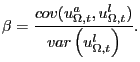
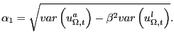
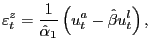
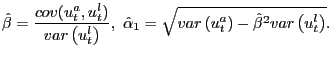
As noted above, CKM's measurement error assumption has the
implication that
![]() is
roughly equals to
is
roughly equals to
![]() To
investigate the role played by this peculiar implication, we delete
To
investigate the role played by this peculiar implication, we delete
![]() from
from
![]() and reestimate
the system. We present the results in the right column of Figure
11. In each panel of that column, we re-estimate the system in the
same way as the corresponding panel in the left column, except that
and reestimate
the system. We present the results in the right column of Figure
11. In each panel of that column, we re-estimate the system in the
same way as the corresponding panel in the left column, except that
![]() is
excluded from
is
excluded from ![]() Comparing the 2,1 and 2,2 panels, we see that, with the May
measurement error specification, the bias disappears after relaxing
CKM's
Comparing the 2,1 and 2,2 panels, we see that, with the May
measurement error specification, the bias disappears after relaxing
CKM's
![]() assumption. Under the July
specification of measurement error, the bias result remains even
after relaxing CKM's assumption (compare the 1,1 and 1,2 graphs of
Figure 11). As noted above, the May specification of CKM's model
has a likelihood that is orders of magnitude higher than the July
specification. So, in the version of the CKM model selected by the
likelihood criterion (i.e., the May version), the
assumption. Under the July
specification of measurement error, the bias result remains even
after relaxing CKM's assumption (compare the 1,1 and 1,2 graphs of
Figure 11). As noted above, the May specification of CKM's model
has a likelihood that is orders of magnitude higher than the July
specification. So, in the version of the CKM model selected by the
likelihood criterion (i.e., the May version), the
![]() assumption plays a central
role in driving the CKM's bias result.
assumption plays a central
role in driving the CKM's bias result.
In sum, CKM's examples which imply that VARs with long-run identification display substantial bias, are not empirically interesting from a likelihood point of view. The bias in their examples is due to the way CKM choose the measurement error variance. When their measurement error specification is tested, it is overwhelmingly rejected in favor of an alternative in which the CKM bias result disappears.
CKM argue that there is considerable uncertainty in the business
cycle literature about the values of parameters governing
stochastic processes such as preferences and technology. They argue
that this uncertainty translates into a wide class of examples in
which the bias in structural VARs leads to severely misleading
inference. The right panel in Figure 12 summarizes their argument.
The horizontal axis covers the range of values of
![]() considered by
CKM. For each value of
considered by
CKM. For each value of
![]() we estimate,
by maximum likelihood, four parameters of the two-shock model:
we estimate,
by maximum likelihood, four parameters of the two-shock model:
![]()
![]()
![]() and
and
![]() .29 We use the estimated model as a data
generating process. The left vertical axis displays the small
sample mean of the corresponding VAR-based estimator of the
contemporaneous response of hours worked to a one-standard
deviation technology shock.
.29 We use the estimated model as a data
generating process. The left vertical axis displays the small
sample mean of the corresponding VAR-based estimator of the
contemporaneous response of hours worked to a one-standard
deviation technology shock.
Based on a review the RBC literature, CKM report that they have
a roughly uniform prior over the different values of
![]() considered in
Figure 12. The figure indicates that for many of these values, the
bias is large (compare the small sample mean, the solid line, with
the true response, the starred line). For example, there is a
noticeable bias in the 2-shock CKM specification, where
considered in
Figure 12. The figure indicates that for many of these values, the
bias is large (compare the small sample mean, the solid line, with
the true response, the starred line). For example, there is a
noticeable bias in the 2-shock CKM specification, where
![]()
We emphasize three points. First, as we stress repeatedly, bias
cannot be viewed in isolation from sampling uncertainty. The two
dashed lines in the figure indicate the 95 percent probability
interval. These intervals are enormous relative to the bias.
Second, not all values of
![]() are equally
likely, and for the ones with greatest likelihood there is little
bias. On the horizontal axis of the left panel of Figure 12, we
display the same range of values of
are equally
likely, and for the ones with greatest likelihood there is little
bias. On the horizontal axis of the left panel of Figure 12, we
display the same range of values of
![]() as in the
right panel. On the vertical axis we report the log-likelihood
value of the associated model. The peak of this likelihood occurs
close to the estimated value in the two-shock MLE specification.
Note how the log-likelihood value drops sharply as we consider
values of
as in the
right panel. On the vertical axis we report the log-likelihood
value of the associated model. The peak of this likelihood occurs
close to the estimated value in the two-shock MLE specification.
Note how the log-likelihood value drops sharply as we consider
values of
![]() away from the
unconstrained maximum likelihood estimate. The vertical bars in the
figure indicate the 95 percent confidence interval for
away from the
unconstrained maximum likelihood estimate. The vertical bars in the
figure indicate the 95 percent confidence interval for
![]() 30 Figure 12 reveals that the confidence
interval is very narrow relative to the range of values considered
by CKM, and that within the interval, the bias is quite small.
30 Figure 12 reveals that the confidence
interval is very narrow relative to the range of values considered
by CKM, and that within the interval, the bias is quite small.
Third, the right axis in the right panel of Figure 12 plots
![]() the percent of
the variance in log hours due to technology, as a function of
the percent of
the variance in log hours due to technology, as a function of
![]() The values
of
The values
of
![]() for which
there is a noticeable bias correspond to model economies where
for which
there is a noticeable bias correspond to model economies where
![]() is less than
is less than
![]() percent. Here,
identifying the effects of a technology shock on hours worked is
tantamount to looking for a needle in a haystack.
percent. Here,
identifying the effects of a technology shock on hours worked is
tantamount to looking for a needle in a haystack.
CKM emphasize comparisons between the true dynamic response function in the data generating process and the response function that an econometrician would estimate using a four-lag VAR with an infinite amount of data. In our own analysis in section 4, we find population calculations with four lag VARs useful for some purposes. However, we do not view the probability limit of a four lag VAR as an interesting metric for measuring the usefulness of structural VARs. In practice econometricians do not have an infinite amount of data. Even if they did, they would certainly not use a fixed lag length. Econometricians determine lag length endogenously and, in a large sample, lag length would grow. If lag lengths grow at the appropriate rate with sample size, VAR-based estimators of impulse response functions are consistent. The interesting issue (to us) is how VAR-based procedures perform in samples of the size that practitioners have at their disposal. This is why we focus on small sample properties like bias and sampling uncertainty.
The potential power of the CKM argument lies in showing that VAR-based procedures are misleading, even under circumstances when everyone would agree that VARs should work well, namely when the econometrician commits no avoidable specification error. The econometrician does, however, commit one unavoidable specification error. The true VAR is infinite ordered, but the econometrician assumes the VAR has a finite number of lags. CKM argue that this seemingly innocuous assumption is fatal for VAR analysis. We have argued that this conclusion is unwarranted.
CKM present other examples in which the econometrician commits an avoidable specification error. Specifically, they study the consequences of over differencing hours worked. That is, the econometrician first differences hours worked when hours worked are stationary.31 This error gives rise to bias in VAR-based impulse response functions that is large relative to sampling uncertainty. CKM argue that this bias is another reason not to use VARs.
However, the observation that avoidable specification error is
possible in VAR analysis is not a problem for VARs per se. The
possibility of specification error is a potential pitfall for any
type of empirical work. In any case, CKM's analysis of the
consequences of over differencing is not new. For example,
Christiano, Eichenbaum and Vigfusson (2003, hereafter, CEV) study a
situation in which the true data generating process satisfies two
properties: Hours worked are stationary and they rise after a
positive technology shock. CEV then consider an econometrician who
does VAR-based long-run identification when ![]() in (16)
contains the growth rate of hours rather than the log level of
hours. CEV show that the econometrician would falsely conclude that
hours worked fall after a positive technology shock. CEV do not
conclude from this exercise that structural VARs are not useful.
Rather, they develop a statistical procedure to help decide whether
hours worked should be first differenced or not.
in (16)
contains the growth rate of hours rather than the log level of
hours. CEV show that the econometrician would falsely conclude that
hours worked fall after a positive technology shock. CEV do not
conclude from this exercise that structural VARs are not useful.
Rather, they develop a statistical procedure to help decide whether
hours worked should be first differenced or not.
We argue that VAR-based short-run identification schemes lead to remarkably accurate and precise inference. This result is of interest because the preponderance of the empirical literature on structural VARs explores the implications of short-run identification schemes. CKM are silent on this literature. McGrattan (2006) dismisses short-run identification schemes as `` hokey.'' One possible interpretation of this adjective is that McGrattan can easily imagine models in which the identification scheme is incorrect. The problem with this interpretation is that all models are a collection of strong identifying assumptions, all of which can be characterized as `` hokey''. A second interpretation is that in McGrattan (2006)'s view, the type of zero restrictions typically used in short run identification are not compatible with dynamic equilibrium theory. This view is simply incorrect (see Sims and Zha (2006)). A third possible interpretation is that no one finds short-run identifying assumptions interesting. However, the results of short-run identification schemes have had an enormous effect on the construction of dynamic, general equilibrium models. See Woodford (2003) for a summary in the context of monetary models.
CKM argue that VARs are very sensitive to the choice of data. Specifically, they review the papers by Francis and Ramey (2004), CEV, and Gali and Rabanal (2004), which use long-run VAR methods to estimate the response of hours worked to a positive technology shock. CKM note that these studies use different measures of per capita hours worked and output in the VAR analysis. The bottom panel of Figure 13 displays the different measures of per capita hours worked that these studies use. Note how the low frequency properties of these series differ. The corresponding estimated impulse response functions and confidence intervals are reported in the top panel. CKM view it as a defect in VAR methodology that the different measures of hours worked lead to different estimated impulse response functions. We disagree. Empirical results should be sensitive to substantial changes in the data. A constructive response to the sensitivity in Figure 13 is to carefully analyze the different measures of hours worked, see which is more appropriate, and perhaps construct a better measure. It is not constructive to dismiss an econometric technique that signals the need for better measurement.
CKM note that the principle differences in the hours data occur in the early part of the sample. According to CKM, when they drop these early observations they obtain different impulse response functions. However, as Figure 13 shows, these impulse response functions are not significantly different from each other.
6 A Model with Nominal Rigidities
In this section we use the model in ACEL to assess the accuracy of structural VARs for estimating the dynamic response of hours worked to shocks. This model allows for nominal rigidities in prices and wages and has three shocks: a monetary policy shock, a neutral technology shock, and a capital-embodied technology shock. Both technology shocks affect labor productivity in the long run. However, the only shock in the model that affects the price of investment in the long run is the capital-embodied technology shock. We use the ACEL model to evaluate the ability of a VAR to uncover the response of hours worked to both types of technology shock and to the monetary policy shock. Our strategy for identifying the two technology shocks is similar to the one proposed by Fisher (2006). The model rationalizes a version of the short-run, recursive identification strategy used by Christiano, Eichenbaum and Evans (1999) to identify monetary shocks. This strategy corresponds closely to the recursive procedure studied in section 2.3.2.
6.1 The Model
The details of the ACEL model, as well as the parameter
estimates, are reported in Appendix A of the NBER Working Paper
version of this paper. Here, we limit our discussion to what is
necessary to clarify the nature of the shocks in the ACEL model.
Final goods, ![]() are
produced using a standard Dixit-Stiglitz aggregator of intermediate
goods,
are
produced using a standard Dixit-Stiglitz aggregator of intermediate
goods,
![]()
![]() To produce
a unit of consumption goods,
To produce
a unit of consumption goods, ![]() one unit of final goods is required. To produce
one unit of investment goods,
one unit of final goods is required. To produce
one unit of investment goods, ![]()
![]() units of final goods are required. In equilibrium,
units of final goods are required. In equilibrium,
![]() is
the price, in units of consumption goods, of an investment good.
Let
is
the price, in units of consumption goods, of an investment good.
Let
![]() denote the growth rate of
denote the growth rate of
![]() let
let
![]() denote
the nonstochastic steady state value of
denote
the nonstochastic steady state value of
![]() and
let
and
let
![]() denote the percent deviation of
denote the percent deviation of
![]() from
its steady state value:
from
its steady state value:

The stochastic process for the growth rate of
We refer to the i.i.d. unit variance random variable,

The stochastic process for the growth rate of
where the i.i.d. unit variance random variable,
We now turn to the monetary policy shock. Let ![]() denote
denote
![]() where
where
![]() denotes the
monetary base. Let
denotes the
monetary base. Let
![]() denote the
percentage deviation of
denote the
percentage deviation of ![]() from its steady state, i.e.,
from its steady state, i.e.,
![]() We
suppose that
We
suppose that
![]() is the sum
of three components. One,
is the sum
of three components. One,
![]() represents the component of
represents the component of
![]() reflecting
an exogenous shock to monetary policy. The other two,
reflecting
an exogenous shock to monetary policy. The other two,
![]() and
and
![]() represent the endogenous response of
represent the endogenous response of
![]() to the
neutral and capital-embodied technology shocks, respectively. Thus
monetary policy is given by:
to the
neutral and capital-embodied technology shocks, respectively. Thus
monetary policy is given by:
ACEL assume that
Here,
Table 3 summarizes the importance of different shocks for the
variance of hours worked and output. Neutral and capital-embodied
technology shocks account for roughly equal percentages of the
variance of hours worked (![]() percent each), while monetary policy shocks account
for the remainder. Working with HP-filtered data reduces the
importance of neutral technology shocks to about
percent each), while monetary policy shocks account
for the remainder. Working with HP-filtered data reduces the
importance of neutral technology shocks to about ![]() percent. Monetary policy shocks
become much more important for the variance of hours worked. A
qualitatively similar picture emerges when we consider output.
percent. Monetary policy shocks
become much more important for the variance of hours worked. A
qualitatively similar picture emerges when we consider output.
It is worth emphasizing that neutral technology shocks are much more important in hours worked in the ACEL model than in the RBC model. This fact plays an important role in determining the precision of VAR-based inference using long-run restrictions in the ACEL model.
6.2 Results
We use the ACEL model to simulate 1,000 data sets each with 180 observations. We report results from two different VARs. In the first VAR, we simultaneously estimate the dynamic effect on hours worked of a neutral technology shock and a capital-embodied technology shock. The variables in this VAR are:
![\begin{displaymath} Y_{t}=\left( \begin{array}[c]{c} \Delta\ln p_{It}\ \Delta\ln a_{t}\ \ln l_{t} \end{array}\right) , \end{displaymath}](img379.gif)
The 1,1 panel of Figure 14 displays our results using the standard VAR procedure to estimate the dynamic response of hours worked to a neutral technology shock. Several results are worth emphasizing. First, the estimator is essentially unbiased. Second, the econometrician's estimator of sampling uncertainty is also reasonably unbiased. The circles and stars, which indicate the mean value of the econometrician's standard-deviation-based and percentile-based confidence intervals, roughly coincide with the boundaries of the gray area. However, there is a slight tendency, in both cases, to understate the degree of sampling uncertainty. Third, confidence intervals are small, relative to those in the RBC examples. Both sets of confidence intervals exclude zero at all lags shown. This result provides another example, in addition to the one provided by Erceg, Guerrieri, and Gust (2005), in which long-run identifying restrictions are useful for discriminating between models. An econometrician who estimates that hours drop after a positive technology shock would reject our parameterization of the ACEL model. Similarly, an econometrician with a model implying that hours fall after a positive technology shock would most likely reject that model if the actual data were generated by our parameterization of the ACEL model.
The 2,1 panel in Figure 14 shows results for the response to a capital-embodied technology shock as estimated using the standard VAR estimator. The sampling uncertainty is somewhat higher for this estimator than for the neutral technology shock. In addition, there is a slight amount of bias. The econometrician understates somewhat the degree of sampling uncertainty.
We now consider the response of hours worked to a monetary policy shock. We estimate this response using a VAR with the following variables:
![\begin{displaymath} Y_{t}=\left( \begin{array}[c]{c} \Delta\log a_{t}\ \log l_{t}\ R_{t} \end{array}\right) . \end{displaymath}](img383.gif)
7 Concluding Remarks
In this paper we study the ability of structural VARs to uncover the response of hours worked to a technology shock. We consider two classes of data generating processes. The first class consists of a series of real business cycle models that we estimate using maximum likelihood methods. The second class consists of the monetary model in ACEL. We find that with short-run restrictions, structural VARs perform remarkably well in all our examples. With long-run restrictions, structural VARs work well as long as technology shocks explain at least a very small portion of the variation in hours worked.
In a number of examples that we consider, VAR-based impulse response functions using long-run restrictions exhibit some bias. Even though these examples do not emerge from empirically plausible data generating processes, we find them of interest. They allow us to diagnose what can go wrong with long-run identification schemes. Our diagnosis leads us to propose a modification to the standard VAR-based procedure for estimating impulse response functions using long-run identification. This procedure works well in our examples.
Finally, we find that confidence intervals with long-run identification schemes are substantially larger than those with short-run identification schemes. In all empirically plausible cases, the VARs deliver confidence intervals that accurately reflect the true degree of sampling uncertainty. We view this characteristic as a great virtue of VAR-based methods. When the data contain little information, the VAR will indicate the lack of information. To reduce large confidence intervals the analyst must either impose additional identifying restrictions (i.e., use more theory) or obtain better data.
References
Altig, David, Lawrence Christiano, Martin Eichenbaum, and Jesper Linde (2005). `` Firm-Specific Capital, Nominal Rigidities, and the Business Cycle,'' NBER Working Paper Series 11034. Cambridge, Mass.: National Bureau of Economic Research, January.
Andrews, Donald W. K., and J. Christopher Monahan (1992). `` An Improved Heteroskedasticity and Autocorrelation Consistent Covariance Matrix Estimator,'' Econometrica , vol. 60 (July), pp. 953-66.
Basu, Susanto, John Fernald, and Miles Kimball (2004). `` Are Technology Improvements Contractionary?'' NBER Working Paper Series 10592. Cambridge, Mass.: National Bureau of Economic Research, June.
Bernanke, Ben S. (1986). `` Alternative Explanations of the Money-Income Correlation,'' Carnegie Rochester Conference Series on Public Policy, vol. 25 (Autumn), pp. 49-99.
Bernanke, Ben S., and Alan S. Blinder (1992). `` The Federal Funds Rate and the Channels of Monetary Transmission,'' American Economic Review, vol. 82 (September), pp. 901-21.
Bernanke, Ben S., and Ilian Mihov (1998). `` Measuring Monetary Policy,'' Quarterly Journal of Economics, vol. 113 (August), pp. 869-902.
Blanchard, Olivier, and Roberto Perotti (2002). `` An Empirical Characterization of the Dynamic Effects of Changes in Government Spending and Taxes on Output,'' Quarterly Journal of Economics, vol. 117 (November), pp. 1329-68.
Blanchard, Olivier, and Danny Quah (1989). `` The Dynamic Effects of Aggregate Demand and Supply Disturbances,'' American Economic Review, vol. 79 (September), pp. 655-73.
Blanchard, Olivier, and Mark Watson (1986). `` Are Business Cycles All Alike?'' in Robert Gordon, ed., Continuity and Change in the American Business Cycle. Chicago: University of Chicago Press, pp.123-56.
Chari, V. V., Patrick J. Kehoe, and Ellen McGrattan (2005a). `` A Critique of Structural VARs Using Real Business Cycle Theory,'' Working Paper Series 631. Minneapolis: Federal Reserve Bank of Minneapolis, May.
----- (2005b). `` A Critique of Structural VARs Using Real Business Cycle Theory,'' Working Paper Series 631. Minneapolis: Federal Reserve Bank of Minneapolis, July.
Christiano, Lawrence J. (1988). `` Why Does Inventory Investment Fluctuate So Much?'' Journal of Monetary Economics, vol. 21 (March-May), pp. 247-80.
----- (2002). `` Solving Dynamic Equilibrium Models by a Method of Undetermined Coefficients,'' Computational Economics, vol. 20 (October), pp. 21-55.
Christiano, Lawrence J., and Martin Eichenbaum (1992). `` Identification and the Liquidity Effect of a Monetary Policy Shock,'' in Alex Cukierman, Zvi Hercowitz, and Leonardo Leiderman, eds., Political Economy, Growth, and Business Cycles. Cambridge, Mass.: MIT Press, pp. 335-70.
Christiano, Lawrence J., Martin Eichenbaum, and Charles Evans (1999). `` Monetary Policy Shocks: What Have We Learned and to What End?,'' in John B.Taylor and Michael D. Woodford, eds., Handbook of Macroeconomics. Volume 1A, Amsterdam; Elsevier Science, pp. 65-148
Christiano, Lawrence J., Martin Eichenbaum, and Charles Evans (2005). `` Nominal Rigidities and the Dynamic Effects of a Shock to Monetary Policy,'' Journal of Political Economy, vol. 113 (February), pp. 1-45.
Christiano, Lawrence J., Martin Eichenbaum, and Robert Vigfusson (2003). `` What Happens after a Technology Shock?'' NBER Working Paper Series 9819. Cambridge, Mass.: National Bureau of Economic Research, July.
----- (2004). `` The Response of Hours to a Technology Shock: Evidence Based on Direct Measures of Technology,'' Journal of the European Economic Association, vol. 2 (April), pp. 381-95.
----- (forthcoming). `` Alternative Procedures for Estimating Long-Run Identified Vector Autoregressions,'' Journal of the European Economic Association.
Cooley, Thomas F., and Mark Dwyer (1998). `` Business Cycle Analysis without Much Theory: A Look at Structural VARs,'' Journal of Econometrics, vol. 83 (March-April), pp. 57-88.
Cushman, David O., and Tao Zha (1997). `` Identifying Monetary Policy in a Small Open Economy under Flexible Exchange Rates,'' Journal of Monetary Economics, vol. 39 (August), pp. 433-48.
Del Negro, Marco, Frank Schorfheide, Frank Smets, and Raf Wouters (2005). `` On the Fit and Forecasting Performance of New Keynesian Models,'' unpublished paper, University of Pennsylvania.
Eichenbaum, Martin, and Charles Evans (1995). `` Some Empirical Evidence on the Effects of Shocks to Monetary Policy on Exchange Rates,'' Quarterly Journal of Economics, vol. 110 (November), pp. 975-1009.
Erceg, Christopher J., Luca Guerrieri, and Christopher Gust (2005). `` Can Long-Run Restrictions Identify Technology Shocks?'' Journal of the European Economic Association, vol. 3 (December), pp. 1237-78.
Faust, Jon, and Eric Leeper (1997). `` When Do Long-Run Identifying Restrictions Give Reliable Results?'' Journal of Business and Economic Statistics, vol. 15 (July), pp. 345-53.
Fernandez-Villaverde, Jesus, Juan F. Rubio-Ramirez, and Thomas J. Sargent (2005). `` A, B, C's (and D's) for Understanding VARs,'' unpublished paper, New York University.
Fisher, Jonas (2006). `` The Dynamic Effects of Neutral and Investment-Specific Technology Shocks,'' Journal of Political Economy, vol. 114, no. 3, June.
Francis, Neville, Michael T. Owyang, and Jennifer E. Roush (2005). `` A Flexible Finite-Horizon Identification of Technology Shocks,'' Working Paper Series 2005-024A. St. Louis: Federal Reserve Bank of St. Louis, April.
Francis, Neville, and Valerie A. Ramey (2005). `` Is the Technology-Driven Real Business Cycle Hypothesis Dead? Shocks and Aggregate Fluctuations Revisited,'' Journal of Monetary Economics, vol. 52 (November), pp. 1379-99.
Gali, Jordi (1999). `` Technology, Employment, and the Business Cycle: Do Technology Shocks Explain Aggregate Fluctuations?'' American Economic Review, vol. 89 (March), pp. 249-71.
Gali, Jordi, and Pau Rabanal (2005). `` Technology Shocks and Aggregate Fluctuations: How Well Does the Real Business Cycle Model Fit Postwar U.S. Data?'' in Mark Gertler and Kenneth Rogoff, eds., NBER Macroeconomics Annual 2004. Cambridge, Mass.: MIT Press.
Hamilton, James D. (1994). Time Series Analysis. Princeton: Princeton University Press.
----- (1997). `` Measuring the Liquidity Effect,'' American Economic Review, vol. 87 (March), pp. 80-97.
Hansen, Lars, and Thomas Sargent (1980). `` Formulating and Estimating Dynamic Linear Rational Expectations Models,'' Journal of Economic Dynamics and Control, vol. 2 (February), pp. 7-46.
King, Robert G., Charles I. Plosser, James H. Stock, and Mark W. Watson (1991). `` Stochastic Trends and Economic Fluctuations,'' American Economic Review, vol. 81 (September), pp. 819-40.
McGrattan, Ellen (2006). `` A Critique of Structural VARs Using Business Cycle Theory,'' presentation at the annual meeting of the American Economic Association, Boston, January 6-8, http://minneapolisfed.org/research/economists/mcgrattan/CEV/assa.htm.
Pagan, Adrian R., and John C. Robertson (1998). `` Structural Models of the Liquidity Effect,'' Review of Economics and Statistics, vol. 80 (May), pp. 202-17.
Ravenna, Federico, 2005, `Vector Autoregressions and Reduced Form Representations of Dynamic Stochastic General Equilibrium Models,' unpublished manuscript.
Rotemberg, Julio J., and Michael Woodford (1992). `` Oligopolistic Pricing and the Effects of Aggregate Demand on Economic Activity,'' Journal of Political Economy, vol. 100 (December), pp. 1153-1207.
----- (1997). `` An Optimization-Based Econometric Framework for the Evaluation of Monetary Policy,'' in Ben S. Bernanke and Julio Rotemberg, eds., NBER Macroeconomics Annual 1997. Cambridge, Mass.: MIT Press.
Runkle, David E. (1987). `` Vector Autoregressions and Reality,'' Journal of Business and Economic Statistics, vol. 5 (October), pp. 437-442.
Shapiro, Matthew, and Mark Watson (1988). `` Sources of Business Cycle Fluctuations,'' in Stanley Fischer, ed., NBER Macroeconomics Annual 1988. Cambridge, Mass.: MIT Press.
Sims, Christopher (1972). `` The Role of Approximate Prior Restrictions in Distributed Lag Estimation,'' Journal of the American Statistical Association, vol. 67 (March), pp. 169-75.
----- (1980). `` Macroeconomics and Reality,'' Econometrica, vol. 48 (January), pp. 1-48.
----- (1986). `` Are Forecasting Models Usable for Policy Analysis?'' Federal Reserve Bank of Minneapolis, Quarterly Review, vol. 10 (Winter), pp. 2-16.
----- (1989). `` Models and Their Uses,'' American Journal of Agricultural Economics, vol. 71 (May), pp. 489-94.
Sims, Christopher, and Tao Zha (1999). `` Error Bands for Impulse Responses,'' Econometrica, vol. 67 (September), pp. 1113-55.
----- (forthcoming). `` Does Monetary Policy Generate Recessions?'' Macroeconomic Dynamics.
Smets, Frank, and Raf Wouters (2003). `` An Estimated Dynamic Stochastic General Equilibrium Model of the Euro Area,'' Journal of the European Economic Association, vol. 1 (September), pp. 1123-75.
Vigfusson, Robert J. (2004). `` The Delayed Response to a Technology Shock: A Flexible Price Explanation,'' International Finance Discussion Paper Series 2004-810. Washington: Board of Governors of the Federal Reserve System, July.
Woodford, Michael M. (2003). Interest and Prices: Foundations of a Theory of Monetary Policy. Princeton: Princeton University Press.
A. A Model with Nominal Wage and Price Rigidities
This appendix describes the ACEL model used in section 6. The model economy is composed of households, firms, and a monetary authority.
There is a continuum of households, indexed by
![]() The
The
![]() household is a
monopoly supplier of a differentiated labor service, and sets its
wage subject to Calvo-style wage frictions. In general, households
earn different wage rates and work different amounts. A
straightforward extension of arguments in Erceg, Henderson, and
Levin (2000) and in Woodford (1996) establishes that in the
presence of state contingent securities, households are homogeneous
with respect to consumption and asset holdings.33 Our notation reflects this result. The
preferences of the
household is a
monopoly supplier of a differentiated labor service, and sets its
wage subject to Calvo-style wage frictions. In general, households
earn different wage rates and work different amounts. A
straightforward extension of arguments in Erceg, Henderson, and
Levin (2000) and in Woodford (1996) establishes that in the
presence of state contingent securities, households are homogeneous
with respect to consumption and asset holdings.33 Our notation reflects this result. The
preferences of the ![]() household are given by:
household are given by:
![$\displaystyle E_{t}^{j}\sum_{l=0}^{\infty}\beta^{l-t}\left[ \log\left( C_{t+l} -bC_{t+l-1}\right) -\psi_{L}\frac{h_{j,t+l}^{2}}{2}\right] , $](img388.gif)
Here,

where
The ![]() household is a monopoly supplier of a differentiated labor service,
household is a monopoly supplier of a differentiated labor service,
![]() . It sells this
service to a representative, competitive firm that transforms it
into an aggregate labor input,
. It sells this
service to a representative, competitive firm that transforms it
into an aggregate labor input, ![]() using the technology:
using the technology:
![$\displaystyle H_{t}=\left[ \int_{0}^{1}h_{j,t}^{\frac{1}{\lambda_{w}}}dj\right] ^{\lambda_{w}},$](img420.gif)
In each period, a household faces a constant probability,
![]() of being
able to re-optimize its nominal wage. The ability to re-optimize is
independent across households and time. If a household cannot
re-optimize its wage at time
of being
able to re-optimize its nominal wage. The ability to re-optimize is
independent across households and time. If a household cannot
re-optimize its wage at time ![]() it sets
it sets ![]() according to:
according to:
At time ![]() a final
consumption good,
a final
consumption good, ![]() is produced by a perfectly competitive, representative final good
firm. This firm produces the final good by combining a continuum of
intermediate goods, indexed by
is produced by a perfectly competitive, representative final good
firm. This firm produces the final good by combining a continuum of
intermediate goods, indexed by
![]() using
the technology
using
the technology
![$\displaystyle Y_{t}=\left[ \int_{0}^{1}y_{t}(i)^{\frac{1}{\lambda_{f}}}di\right] ^{\lambda_{f}},$](img431.gif)
where
Intermediate good ![]() is
produced by a monopolist using the following technology:
is
produced by a monopolist using the following technology:
![$\displaystyle y_{t}(i)=\left\{ \begin{array}[c]{ll} K_{t}(i)^{\alpha}\left( Z_{... ...ht) ^{1-\alpha}\geq\phi z_{t}^{\ast}\\ 0 & \text{otherwise} \end{array} \right.$](img438.gif)
where
where
Intermediate good firms hire labor in perfectly competitive
factor markets at the wage rate, ![]() . Profits are distributed to households at the
end of each time period. We assume that the firm must borrow the
wage bill in advance at the gross interest rate,
. Profits are distributed to households at the
end of each time period. We assume that the firm must borrow the
wage bill in advance at the gross interest rate, ![]()
In each period, the ![]() intermediate goods firm faces a constant
probability,
intermediate goods firm faces a constant
probability,
![]() of being
able to re-optimize its nominal price. The ability to re-optimize
prices is independent across firms and time. If firm
of being
able to re-optimize its nominal price. The ability to re-optimize
prices is independent across firms and time. If firm ![]() cannot re-optimize, it sets
cannot re-optimize, it sets
![]() according
to:
according
to:
Let
![]() denote the physical stock
of capital available to the
denote the physical stock
of capital available to the ![]() firm at the beginning of period
firm at the beginning of period ![]() The services of capital,
The services of capital,
![]() are related to stock of physical capital, by:
are related to stock of physical capital, by:
There is no technology for transferring capital between firms.
The only way a firm can change its stock of physical capital is by
varying the rate of investment,
![]() over time. The technology for accumulating physical capital by
intermediate good firm
over time. The technology for accumulating physical capital by
intermediate good firm ![]() is given by:
is given by:
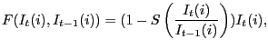
The present discounted value of the ![]() intermediate good's net cash
flow is given by:
intermediate good's net cash
flow is given by:
![$\displaystyle E_{t}\sum_{j=0}^{\infty}\beta^{j}\upsilon_{t+j}\left\{ P_{t+j}(i)... ...\left[ I_{t+j} (i)+a\left( u_{t+j}(i)\right) \bar{K}_{t+j}(i)\right] \right\} ,$](img470.gif)
where
The monetary policy rule is defined by (35)
and (36). Financial intermediaries receive
![]() from the
household. Our notation reflects the equilibrium condition,
from the
household. Our notation reflects the equilibrium condition,
![]() Financial intermediaries lend all of their money to intermediate
good firms, which use the funds to pay labor wages. Loan market
clearing requires that:
Financial intermediaries lend all of their money to intermediate
good firms, which use the funds to pay labor wages. Loan market
clearing requires that:
The aggregate resource constraint is:
We refer the reader to ACEL for a description of how the model is solved and for the methodology used to estimate the model parameters. The data and programs, as well as an extensive technical appendix, may be found at the following website:
www.faculty.econ.northwestern.edu/faculty/christiano/research/ACEL/acelweb.htm.
B. Long-Run Identification of Two Technology Shocks
This appendix generalizes the strategy for long-run identification of one shock to two shocks, using the strategy of Fisher (2006). As before, the VAR is:
We suppose that the fundamental shocks are related to the VAR disturbances as follows:
That is, only technology shocks have a long-run effect on the log-level of labor productivity, whereas only capital-embodied shocks have a long-run effect on the log-level of the price of investment goods. According to the sign restrictions, the slope of
![\begin{displaymath} \left[ I-B(1)\right] ^{-1}C=\left[ \begin{array}[c]{ccc} a &... ...ext{number} & \text{number} & \text{number} \end{array}\right] \end{displaymath}](img486.gif)
where, as before,
![\begin{displaymath} D=\left[ \begin{array}[c]{ccc} d_{11} & 0 & 0\ d_{21} & d_{22} & 0\ d_{31} & d_{32} & d_{33} \end{array}\right] . \end{displaymath}](img490.gif)
![\begin{displaymath} DD^{\prime}=\left[ \begin{array}[c]{ccc} d_{11}^{2} & d_{11}... ...\left( 0\right) & S_{Y}^{33}\left( 0\right) \end{array}\right] \end{displaymath}](img492.gif)
|
The sign restrictions imply that the square roots should be positive. The fact that
![$\displaystyle \left[ C_{1}\vdots C_{2}\right] =\left[ I-B(1)\right] \left[ D_{1}\vdots D_{2}\right] , $](img500.gif)
To construct our modified VAR procedure, simply replace
![]() in (45) by (29).
in (45) by (29).
Figure 1: A Simulated Time Series for Hours
Data for Figure 1: A Simulated Time Series for Hours
Time |
Two-Shock MLE Specification: Both shocks, ln(hours) | Two-Shock MLE Specification: Only Technology Shocks, ln(hours) | Two-Shock CKM Specification: Both Shocks, ln(hours) | Two-Shock CKM Specification: Only Technology Shocks, ln(hours) |
|---|---|---|---|---|
| 1 | -1.57346 | -1.56093 | -1.54288 | -1.55774 |
| 2 | -1.58337 | -1.5605 | -1.57193 | -1.55714 |
| 3 | -1.58809 | -1.55865 | -1.58755 | -1.5546 |
| 4 | -1.59002 | -1.55497 | -1.59738 | -1.54955 |
| 5 | -1.58387 | -1.55489 | -1.57951 | -1.54944 |
| 6 | -1.59784 | -1.55268 | -1.6205 | -1.5464 |
| 7 | -1.59196 | -1.55952 | -1.59292 | -1.5558 |
| 8 | -1.60947 | -1.5581 | -1.64233 | -1.55385 |
| 9 | -1.6063 | -1.56053 | -1.62777 | -1.55719 |
| 10 | -1.60639 | -1.56131 | -1.62512 | -1.55826 |
| 11 | -1.59256 | -1.55975 | -1.58758 | -1.55612 |
| 12 | -1.60073 | -1.55848 | -1.61142 | -1.55437 |
| 13 | -1.60544 | -1.55861 | -1.62289 | -1.55455 |
| 14 | -1.61011 | -1.56303 | -1.62795 | -1.56062 |
| 15 | -1.60276 | -1.56192 | -1.60768 | -1.5591 |
| 16 | -1.59233 | -1.56456 | -1.57447 | -1.56272 |
| 17 | -1.5918 | -1.56665 | -1.57059 | -1.56559 |
| 18 | -1.58706 | -1.56767 | -1.55683 | -1.56699 |
| 19 | -1.59596 | -1.56688 | -1.5836 | -1.5659 |
| 20 | -1.59523 | -1.56682 | -1.58186 | -1.56582 |
| 21 | -1.59475 | -1.56936 | -1.57728 | -1.56931 |
| 22 | -1.58534 | -1.56511 | -1.5578 | -1.56348 |
| 23 | -1.59005 | -1.56434 | -1.57283 | -1.56242 |
| 24 | -1.60655 | -1.56916 | -1.61197 | -1.56904 |
| 25 | -1.60882 | -1.56731 | -1.61997 | -1.5665 |
| 26 | -1.60803 | -1.57046 | -1.61234 | -1.57082 |
| 27 | -1.60814 | -1.57055 | -1.61182 | -1.57094 |
| 28 | -1.60282 | -1.56997 | -1.59733 | -1.57015 |
| 29 | -1.61685 | -1.5716 | -1.63348 | -1.57239 |
| 30 | -1.60214 | -1.57278 | -1.59006 | -1.57401 |
| 31 | -1.60858 | -1.57194 | -1.60919 | -1.57285 |
| 32 | -1.59613 | -1.56909 | -1.57843 | -1.56894 |
| 33 | -1.60963 | -1.56958 | -1.61537 | -1.56961 |
| 34 | -1.61503 | -1.56856 | -1.63079 | -1.56821 |
| 35 | -1.62583 | -1.57122 | -1.65539 | -1.57186 |
| 36 | -1.62128 | -1.5716 | -1.6402 | -1.57238 |
| 37 | -1.61537 | -1.57097 | -1.62327 | -1.57152 |
| 38 | -1.61601 | -1.56937 | -1.62624 | -1.56933 |
| 39 | -1.60415 | -1.57001 | -1.59165 | -1.5702 |
| 40 | -1.61106 | -1.57231 | -1.60766 | -1.57336 |
| 41 | -1.61268 | -1.57713 | -1.60519 | -1.57998 |
| 42 | -1.61087 | -1.57651 | -1.60111 | -1.57912 |
| 43 | -1.60225 | -1.57822 | -1.57523 | -1.58148 |
| 44 | -1.60623 | -1.57869 | -1.5867 | -1.58212 |
| 45 | -1.59319 | -1.5763 | -1.55494 | -1.57884 |
| 46 | -1.58248 | -1.57832 | -1.52456 | -1.58161 |
| 47 | -1.58525 | -1.57772 | -1.53598 | -1.58079 |
| 48 | -1.57366 | -1.57358 | -1.51233 | -1.5751 |
| 49 | -1.56778 | -1.57494 | -1.49744 | -1.57697 |
| 50 | -1.55676 | -1.57448 | -1.4715 | -1.57634 |
| 51 | -1.56001 | -1.577 | -1.48156 | -1.5798 |
| 52 | -1.54993 | -1.57305 | -1.46357 | -1.57438 |
| 53 | -1.55138 | -1.57187 | -1.47384 | -1.57276 |
| 54 | -1.55105 | -1.56798 | -1.48248 | -1.56741 |
| 55 | -1.53253 | -1.56954 | -1.43309 | -1.56956 |
| 56 | -1.53606 | -1.57279 | -1.44378 | -1.57402 |
| 57 | -1.52905 | -1.57079 | -1.43246 | -1.57127 |
| 58 | -1.54096 | -1.57531 | -1.46436 | -1.57748 |
| 59 | -1.53165 | -1.57021 | -1.4502 | -1.57048 |
| 60 | -1.52313 | -1.56594 | -1.43727 | -1.56461 |
| 61 | -1.52199 | -1.56768 | -1.43657 | -1.567 |
| 62 | -1.52176 | -1.57016 | -1.43738 | -1.5704 |
| 63 | -1.5289 | -1.57336 | -1.4575 | -1.5748 |
| 64 | -1.51957 | -1.57329 | -1.4362 | -1.5747 |
| 65 | -1.51828 | -1.57658 | -1.43313 | -1.57922 |
| 66 | -1.51638 | -1.57635 | -1.43341 | -1.5789 |
| 67 | -1.52266 | -1.57556 | -1.45683 | -1.57782 |
| 68 | -1.51537 | -1.57303 | -1.44442 | -1.57435 |
| 69 | -1.51154 | -1.57133 | -1.44064 | -1.57202 |
| 70 | -1.5123 | -1.56899 | -1.45037 | -1.5688 |
| 71 | -1.51228 | -1.56548 | -1.459 | -1.56398 |
| 72 | -1.51973 | -1.56489 | -1.48361 | -1.56317 |
| 73 | -1.52839 | -1.56613 | -1.50807 | -1.56487 |
| 74 | -1.52732 | -1.56806 | -1.50399 | -1.56752 |
| 75 | -1.52123 | -1.5703 | -1.48589 | -1.5706 |
| 76 | -1.51916 | -1.57298 | -1.479 | -1.57428 |
| 77 | -1.53729 | -1.57217 | -1.53275 | -1.57316 |
| 78 | -1.5302 | -1.5716 | -1.51484 | -1.57238 |
| 79 | -1.5178 | -1.57183 | -1.48187 | -1.57271 |
| 80 | -1.51569 | -1.57467 | -1.47477 | -1.5766 |
| 81 | -1.50516 | -1.57259 | -1.45165 | -1.57375 |
| 82 | -1.50613 | -1.56997 | -1.46158 | -1.57015 |
| 83 | -1.50712 | -1.57208 | -1.46455 | -1.57304 |
| 84 | -1.49811 | -1.56965 | -1.44623 | -1.56971 |
| 85 | -1.50877 | -1.56817 | -1.48112 | -1.56768 |
| 86 | -1.50747 | -1.56568 | -1.48318 | -1.56425 |
| 87 | -1.50255 | -1.56441 | -1.47336 | -1.56252 |
| 88 | -1.50314 | -1.56195 | -1.4806 | -1.55913 |
| 89 | -1.50444 | -1.5606 | -1.48784 | -1.55728 |
| 90 | -1.49878 | -1.56041 | -1.474 | -1.55703 |
| 91 | -1.49284 | -1.55987 | -1.46038 | -1.55627 |
| 92 | -1.48933 | -1.56291 | -1.44892 | -1.56045 |
| 93 | -1.48503 | -1.56036 | -1.44355 | -1.55695 |
| 94 | -1.47852 | -1.561 | -1.42773 | -1.55783 |
| 95 | -1.49108 | -1.56141 | -1.46518 | -1.55839 |
| 96 | -1.47872 | -1.55997 | -1.43533 | -1.55642 |
| 97 | -1.47965 | -1.55819 | -1.44344 | -1.55397 |
| 98 | -1.48673 | -1.56367 | -1.45806 | -1.56149 |
| 99 | -1.4972 | -1.56264 | -1.49064 | -1.56008 |
| 100 | -1.51597 | -1.56349 | -1.54213 | -1.56125 |
| 101 | -1.50403 | -1.56616 | -1.50495 | -1.56491 |
| 102 | -1.51362 | -1.56411 | -1.53487 | -1.5621 |
| 103 | -1.52539 | -1.56377 | -1.56723 | -1.56163 |
| 104 | -1.52507 | -1.56415 | -1.5642 | -1.56216 |
| 105 | -1.52725 | -1.56393 | -1.56903 | -1.56185 |
| 106 | -1.54459 | -1.564 | -1.61489 | -1.56195 |
| 107 | -1.54746 | -1.5661 | -1.61661 | -1.56483 |
| 108 | -1.53566 | -1.5643 | -1.58344 | -1.56236 |
| 109 | -1.53471 | -1.56212 | -1.58176 | -1.55937 |
| 110 | -1.52884 | -1.56617 | -1.55797 | -1.56493 |
| 111 | -1.5382 | -1.56551 | -1.58361 | -1.56402 |
| 112 | -1.55043 | -1.57099 | -1.60775 | -1.57155 |
| 113 | -1.53006 | -1.57225 | -1.54752 | -1.57328 |
| 114 | -1.52914 | -1.57379 | -1.54266 | -1.57539 |
| 115 | -1.52378 | -1.57118 | -1.53153 | -1.57181 |
| 116 | -1.52202 | -1.56656 | -1.53333 | -1.56547 |
| 117 | -1.52992 | -1.56825 | -1.55271 | -1.56778 |
| 118 | -1.51915 | -1.5676 | -1.52338 | -1.5669 |
| 119 | -1.51676 | -1.56891 | -1.51546 | -1.56869 |
| 120 | -1.52094 | -1.57114 | -1.52465 | -1.57176 |
| 121 | -1.51878 | -1.56908 | -1.52209 | -1.56892 |
| 122 | -1.51218 | -1.56876 | -1.50489 | -1.56848 |
| 123 | -1.50779 | -1.57257 | -1.48874 | -1.57372 |
| 124 | -1.51508 | -1.57581 | -1.5062 | -1.57816 |
| 125 | -1.5309 | -1.578 | -1.54802 | -1.58118 |
| 126 | -1.52722 | -1.58007 | -1.53502 | -1.58402 |
| 127 | -1.53126 | -1.58039 | -1.54622 | -1.58446 |
| 128 | -1.51024 | -1.5784 | -1.49134 | -1.58172 |
| 129 | -1.49767 | -1.57788 | -1.45956 | -1.58101 |
| 130 | -1.50036 | -1.57574 | -1.47301 | -1.57807 |
| 131 | -1.51285 | -1.57925 | -1.50502 | -1.58289 |
| 132 | -1.50385 | -1.5805 | -1.48006 | -1.5846 |
| 133 | -1.50698 | -1.57414 | -1.49983 | -1.57588 |
| 134 | -1.51393 | -1.57665 | -1.51681 | -1.57933 |
| 135 | -1.511 | -1.5743 | -1.51286 | -1.57609 |
| 136 | -1.51532 | -1.57135 | -1.52964 | -1.57204 |
| 137 | -1.50779 | -1.5742 | -1.50512 | -1.57595 |
| 138 | -1.51453 | -1.57344 | -1.52582 | -1.57492 |
| 139 | -1.50526 | -1.5711 | -1.50388 | -1.5717 |
| 140 | -1.50822 | -1.57238 | -1.51124 | -1.57346 |
| 141 | -1.50994 | -1.57299 | -1.51592 | -1.57429 |
| 142 | -1.50369 | -1.57157 | -1.50134 | -1.57235 |
| 143 | -1.50943 | -1.56816 | -1.52287 | -1.56766 |
| 144 | -1.50481 | -1.56693 | -1.51199 | -1.56597 |
| 145 | -1.5158 | -1.56562 | -1.54442 | -1.56417 |
| 146 | -1.52346 | -1.56365 | -1.56736 | -1.56146 |
| 147 | -1.52042 | -1.56534 | -1.55495 | -1.56378 |
| 148 | -1.52118 | -1.56572 | -1.55534 | -1.56431 |
| 149 | -1.51791 | -1.56697 | -1.54346 | -1.56603 |
| 150 | -1.52661 | -1.56629 | -1.56765 | -1.5651 |
| 151 | -1.51524 | -1.5637 | -1.53842 | -1.56154 |
| 152 | -1.52396 | -1.56218 | -1.56386 | -1.55945 |
| 153 | -1.52228 | -1.56315 | -1.55632 | -1.56079 |
| 154 | -1.52871 | -1.56171 | -1.57469 | -1.5588 |
| 155 | -1.52939 | -1.56025 | -1.57658 | -1.55679 |
| 156 | -1.5448 | -1.56237 | -1.61391 | -1.55971 |
| 157 | -1.54997 | -1.56442 | -1.62197 | -1.56252 |
| 158 | -1.52977 | -1.56648 | -1.56016 | -1.56535 |
| 159 | -1.53532 | -1.56663 | -1.57413 | -1.56556 |
| 160 | -1.53089 | -1.5629 | -1.56551 | -1.56044 |
| 161 | -1.51606 | -1.56063 | -1.52647 | -1.55732 |
| 162 | -1.52319 | -1.56314 | -1.54252 | -1.56078 |
| 163 | -1.51984 | -1.56239 | -1.53381 | -1.55974 |
| 164 | -1.52843 | -1.56419 | -1.55467 | -1.5622 |
| 165 | -1.51793 | -1.56372 | -1.52554 | -1.56157 |
| 166 | -1.52436 | -1.56611 | -1.54005 | -1.56484 |
| 167 | -1.52852 | -1.56447 | -1.55343 | -1.5626 |
| 168 | -1.53991 | -1.56534 | -1.58267 | -1.56379 |
| 169 | -1.54662 | -1.56552 | -1.599 | -1.56403 |
| 170 | -1.53981 | -1.56344 | -1.58071 | -1.56119 |
| 171 | -1.53925 | -1.56352 | -1.57723 | -1.56129 |
| 172 | -1.54097 | -1.56901 | -1.57273 | -1.56883 |
| 173 | -1.5352 | -1.57327 | -1.54979 | -1.57468 |
| 174 | -1.52825 | -1.57468 | -1.52862 | -1.57662 |
| 175 | -1.53071 | -1.57565 | -1.53474 | -1.57795 |
| 176 | -1.53992 | -1.57869 | -1.55638 | -1.58211 |
| 177 | -1.53134 | -1.57532 | -1.5373 | -1.5775 |
| 178 | -1.53506 | -1.57776 | -1.54455 | -1.58085 |
| 179 | -1.53675 | -1.57903 | -1.54768 | -1.58259 |
| 180 | -1.54383 | -1.57625 | -1.57115 | -1.57878 |
Figure 2: Short-run Identification Results
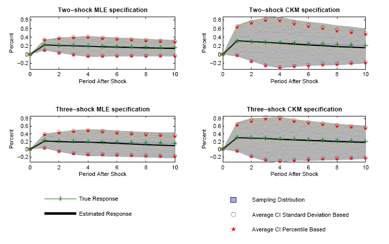
Data for Figure 2: Short-run Identification Results
Two-shock MLE specification (percent):
| Period After Shock | Response: TRUE | Response: Estimated | Sampling Distribution: Lower Bound | Sampling Distribution: Upper Bound | Average CI Standard Deviation Based: Lower Bound | Average CI Standard Deviation Based: Upper Bound | Average CI Percentile Based: Lower Bound | Average CI Percentile Based: Upper Bound |
|---|---|---|---|---|---|---|---|---|
| 0 | 0 | 0 | 0 | 0 | 0 | 0 | 0 | 0 |
| 1 | 0.224817 | 0.220434 | 0.098599 | 0.337069 | 0.097945 | 0.342924 | 0.090327 | 0.330482 |
| 2 | 0.215228 | 0.2079 | 0.039281 | 0.383645 | 0.037362 | 0.378438 | 0.02747 | 0.361311 |
| 3 | 0.206048 | 0.200182 | -0.01286 | 0.400865 | -0.0032 | 0.403564 | -0.01473 | 0.383115 |
| 4 | 0.197259 | 0.18902 | -0.05212 | 0.417773 | -0.03497 | 0.41301 | -0.04918 | 0.389581 |
| 5 | 0.188845 | 0.179063 | -0.04676 | 0.400474 | -0.0301 | 0.388226 | -0.04557 | 0.364014 |
| 6 | 0.18079 | 0.169726 | -0.04336 | 0.383369 | -0.02888 | 0.368333 | -0.04555 | 0.344396 |
| 7 | 0.173079 | 0.162209 | -0.04279 | 0.371952 | -0.02709 | 0.351512 | -0.04393 | 0.328352 |
| 8 | 0.165696 | 0.152485 | -0.04527 | 0.352999 | -0.02816 | 0.333134 | -0.04659 | 0.308549 |
| 9 | 0.158629 | 0.145963 | -0.03891 | 0.341741 | -0.02664 | 0.318566 | -0.04382 | 0.294886 |
| 10 | 0.151863 | 0.13846 | -0.03827 | 0.328068 | -0.02669 | 0.303609 | -0.04329 | 0.280302 |
Two-shock CKM specification (percent):
| Period After Shock | Response: TRUE | Response: Estimated | Sampling Distribution: Lower Bound | Sampling Distribution: Upper Bound | Average CI Standard Deviation Based: Lower Bound | Average CI Standard Deviation Based: Upper Bound | Average CI Percentile Based: Lower Bound | Average CI Percentile Based: Upper Bound |
|---|---|---|---|---|---|---|---|---|
| 0 | 0 | 0 | 0 | 0 | 0 | 0 | 0 | 0 |
| 1 | 0.308693 | 0.314592 | -0.04254 | 0.673878 | -0.01805 | 0.647234 | -0.02779 | 0.623804 |
| 2 | 0.295526 | 0.295759 | -0.15234 | 0.783033 | -0.15649 | 0.74801 | -0.16729 | 0.717305 |
| 3 | 0.282921 | 0.281186 | -0.25529 | 0.845505 | -0.25329 | 0.815666 | -0.26638 | 0.78063 |
| 4 | 0.270853 | 0.260686 | -0.31303 | 0.866041 | -0.29426 | 0.815632 | -0.31242 | 0.773652 |
| 5 | 0.2593 | 0.238182 | -0.284 | 0.793435 | -0.26321 | 0.739571 | -0.28485 | 0.69847 |
| 6 | 0.24824 | 0.218456 | -0.25879 | 0.751611 | -0.24347 | 0.680386 | -0.26833 | 0.640736 |
| 7 | 0.237652 | 0.202869 | -0.25245 | 0.714697 | -0.22241 | 0.62815 | -0.24698 | 0.593162 |
| 8 | 0.227515 | 0.181005 | -0.24496 | 0.666628 | -0.20977 | 0.571779 | -0.23657 | 0.535228 |
| 9 | 0.217811 | 0.168637 | -0.22516 | 0.635865 | -0.19168 | 0.528953 | -0.21241 | 0.499599 |
| 10 | 0.20852 | 0.155345 | -0.20497 | 0.590961 | -0.17709 | 0.487783 | -0.19451 | 0.462818 |
Three-shock MLE specification (percent):
| Period After Shock | Response: TRUE | Response: Estimated | Sampling Distribution: Lower Bound | Sampling Distribution: Upper Bound | Average CI Standard Deviation Based: Lower Bound | Average CI Standard Deviation Based: Upper Bound | Average CI Percentile Based: Lower Bound | Average CI Percentile Based: Upper Bound |
|---|---|---|---|---|---|---|---|---|
| 0 | 0 | 2.26E-18 | -7E-17 | 7.76E-17 | -5.3E-17 | 5.71E-17 | -5.9E-17 | 6.14E-17 |
| 1 | 0.221812 | 0.21271 | 0.028786 | 0.400301 | 0.032151 | 0.39327 | 0.022389 | 0.375947 |
| 2 | 0.212351 | 0.197342 | -0.06132 | 0.445025 | -0.05106 | 0.445744 | -0.06409 | 0.421712 |
| 3 | 0.203294 | 0.185881 | -0.13224 | 0.492192 | -0.10853 | 0.480296 | -0.12355 | 0.453656 |
| 4 | 0.194622 | 0.183614 | -0.17631 | 0.513344 | -0.13496 | 0.502187 | -0.14997 | 0.473984 |
| 5 | 0.186321 | 0.169369 | -0.18177 | 0.507313 | -0.13459 | 0.47333 | -0.15165 | 0.443525 |
| 6 | 0.178374 | 0.151232 | -0.19338 | 0.478514 | -0.14119 | 0.443653 | -0.16079 | 0.413848 |
| 7 | 0.170765 | 0.134955 | -0.19966 | 0.45798 | -0.1497 | 0.41961 | -0.16993 | 0.390676 |
| 8 | 0.163482 | 0.116794 | -0.21185 | 0.442209 | -0.16213 | 0.395715 | -0.18421 | 0.365182 |
| 9 | 0.156509 | 0.104316 | -0.22515 | 0.430158 | -0.16943 | 0.378062 | -0.18921 | 0.350317 |
| 10 | 0.149833 | 0.091458 | -0.23089 | 0.434803 | -0.177 | 0.359915 | -0.1959 | 0.333271 |
Three-shock CKM specification (percent):
| Period After Shock | Response: TRUE | Response: Estimated | Sampling Distribution: Lower Bound | Sampling Distribution: Upper Bound | Average CI Standard Deviation Based: Lower Bound | Average CI Standard Deviation Based: Upper Bound | Average CI Percentile Based: Lower Bound | Average CI Percentile Based: Upper Bound |
|---|---|---|---|---|---|---|---|---|
| 0 | 0 | -7.9E-18 | -9.5E-17 | 0 | -6.4E-17 | 4.82E-17 | -8.3E-17 | 3.92E-17 |
| 1 | 0.308693 | 0.302079 | -0.06073 | 0.692116 | -0.04332 | 0.647474 | -0.05725 | 0.621147 |
| 2 | 0.295526 | 0.288764 | -0.2043 | 0.800781 | -0.17862 | 0.756148 | -0.1972 | 0.717048 |
| 3 | 0.282921 | 0.279528 | -0.30843 | 0.81611 | -0.26766 | 0.826717 | -0.28859 | 0.783652 |
| 4 | 0.270853 | 0.258725 | -0.34187 | 0.843412 | -0.30685 | 0.824295 | -0.32684 | 0.781213 |
| 5 | 0.2593 | 0.241813 | -0.29098 | 0.77331 | -0.27768 | 0.76131 | -0.30129 | 0.720517 |
| 6 | 0.24824 | 0.226933 | -0.3035 | 0.732467 | -0.25613 | 0.709991 | -0.27994 | 0.671858 |
| 7 | 0.237652 | 0.214981 | -0.28693 | 0.699766 | -0.24037 | 0.670333 | -0.26315 | 0.635784 |
| 8 | 0.227515 | 0.197313 | -0.27941 | 0.658455 | -0.23445 | 0.629075 | -0.25843 | 0.593517 |
| 9 | 0.217811 | 0.187768 | -0.26733 | 0.627373 | -0.224 | 0.599539 | -0.24221 | 0.569403 |
| 10 | 0.20852 | 0.176062 | -0.25425 | 0.605437 | -0.21766 | 0.569781 | -0.2331 | 0.542569 |
Figure 3: Coverage Rates, Percentile-Based Confidence Intervals
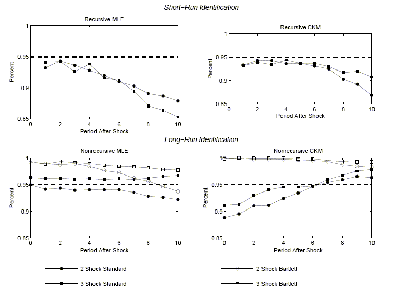
Data for Figure 3: Coverage Rates, Percentile-Based Confidence Intervals
Short-Run Identification (percent):
| Period After Shock | Recursive MLE: .95 line | Recursive MLE: 2 Shock Standard | Recursive MLE: 3 Shock Standard | Recursive CKM: .95 line | Recursive CKM: 2 Shock Standard | Recursive CKM: 3 Shock Standard |
|---|---|---|---|---|---|---|
| 0 | 0.95 | 0.95 | ||||
| 1 | 0.95 | 0.932 | 0.941 | 0.95 | 0.933 | 0.932 |
| 2 | 0.95 | 0.943 | 0.942 | 0.95 | 0.943 | 0.939 |
| 3 | 0.95 | 0.936 | 0.926 | 0.95 | 0.943 | 0.934 |
| 4 | 0.95 | 0.928 | 0.938 | 0.95 | 0.936 | 0.944 |
| 5 | 0.95 | 0.92 | 0.916 | 0.95 | 0.937 | 0.937 |
| 6 | 0.95 | 0.91 | 0.912 | 0.95 | 0.931 | 0.937 |
| 7 | 0.95 | 0.903 | 0.895 | 0.95 | 0.925 | 0.93 |
| 8 | 0.95 | 0.891 | 0.871 | 0.95 | 0.903 | 0.917 |
| 9 | 0.95 | 0.887 | 0.864 | 0.95 | 0.892 | 0.92 |
| 10 | 0.95 | 0.879 | 0.853 | 0.95 | 0.869 | 0.908 |
Long-Run Identification (percent):
| Period After Shock | Nonrecursive MLE: .95 line | Nonrecursive MLE: 2 Shock Standard | Nonrecursive MLE: 2 Shock Bartlett | Nonrecursive MLE: 3 Shock Standard | Nonrecursive MLE: 3 Shock Bartlett | Nonrecursive CKM: .95 line | Nonrecursive CKM: 2 Shock Standard | Nonrecursive CKM: 2 Shock Bartlett | Nonrecursive CKM: 3 Shock Standard | Nonrecursive CKM: 3 Shock Bartlett |
|---|---|---|---|---|---|---|---|---|---|---|
| 0 | 0.95 | 0.949 | 0.991 | 0.963 | 0.993 | 0.95 | 0.888 | 0.999 | 0.911 | 0.998 |
| 1 | 0.95 | 0.941 | 0.989 | 0.961 | 0.988 | 0.95 | 0.895 | 0.999 | 0.913 | 1 |
| 2 | 0.95 | 0.943 | 0.987 | 0.962 | 0.993 | 0.95 | 0.91 | 0.997 | 0.929 | 0.999 |
| 3 | 0.95 | 0.939 | 0.989 | 0.96 | 0.991 | 0.95 | 0.911 | 0.997 | 0.94 | 0.999 |
| 4 | 0.95 | 0.94 | 0.984 | 0.961 | 0.989 | 0.95 | 0.924 | 0.997 | 0.945 | 0.999 |
| 5 | 0.95 | 0.94 | 0.976 | 0.959 | 0.986 | 0.95 | 0.934 | 0.996 | 0.945 | 0.998 |
| 6 | 0.95 | 0.94 | 0.972 | 0.961 | 0.984 | 0.95 | 0.946 | 0.995 | 0.947 | 0.998 |
| 7 | 0.95 | 0.935 | 0.962 | 0.959 | 0.983 | 0.95 | 0.954 | 0.993 | 0.959 | 0.995 |
| 8 | 0.95 | 0.928 | 0.956 | 0.962 | 0.981 | 0.95 | 0.959 | 0.987 | 0.967 | 0.993 |
| 9 | 0.95 | 0.926 | 0.946 | 0.965 | 0.978 | 0.95 | 0.965 | 0.984 | 0.975 | 0.992 |
| 10 | 0.95 | 0.922 | 0.937 | 0.967 | 0.977 | 0.95 | 0.963 | 0.982 | 0.978 | 0.992 |
Figure 4: Coverage Rates, Standard Deviation-Based Confidence Intervals
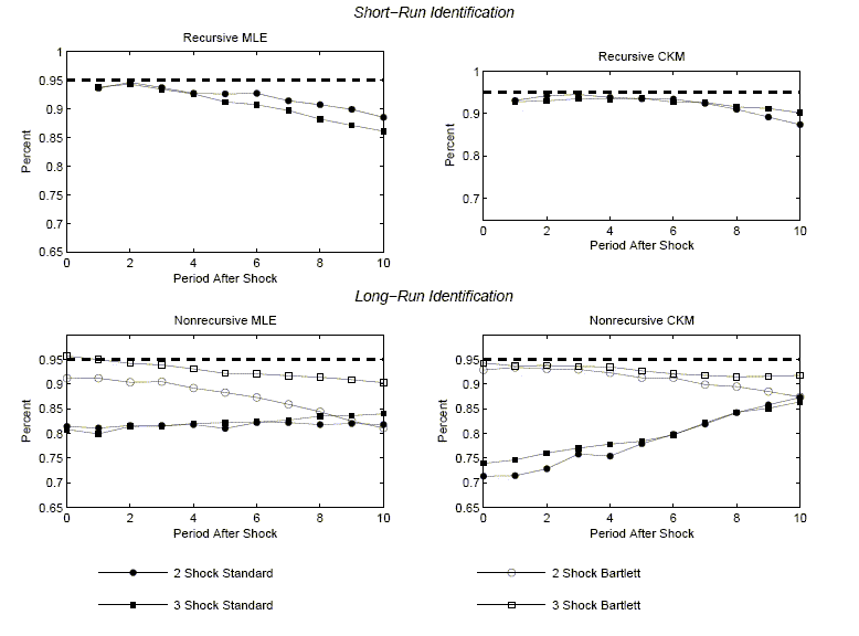
Data for Figure 4: Coverage Rates, Standard Deviation-Based Confidence Intervals
Short-run Identification (percent):
| Period after shock | Recursive MLE: .95 percent | Recursive MLE: 2 Shock Standard | Recursive MLE: 3 Shock Standard | Recursive CKM: .95 percent | Recursive CKM: 2 Shock Standard | Recursive CKM: 3 Shock Standard |
|---|---|---|---|---|---|---|
| 0 | 0.95 | 0.95 | ||||
| 1 | 0.95 | 0.936 | 0.938 | 0.95 | 0.931 | 0.928 |
| 2 | 0.95 | 0.946 | 0.943 | 0.95 | 0.942 | 0.93 |
| 3 | 0.95 | 0.937 | 0.934 | 0.95 | 0.945 | 0.935 |
| 4 | 0.95 | 0.927 | 0.926 | 0.95 | 0.938 | 0.934 |
| 5 | 0.95 | 0.926 | 0.912 | 0.95 | 0.935 | 0.936 |
| 6 | 0.95 | 0.927 | 0.907 | 0.95 | 0.934 | 0.927 |
| 7 | 0.95 | 0.914 | 0.897 | 0.95 | 0.924 | 0.926 |
| 8 | 0.95 | 0.907 | 0.882 | 0.95 | 0.91 | 0.916 |
| 9 | 0.95 | 0.899 | 0.871 | 0.95 | 0.892 | 0.912 |
| 10 | 0.95 | 0.885 | 0.861 | 0.95 | 0.874 | 0.902 |
Long-run Identification (percent):
| Period after shock | Nonrecursive MLE: .95 percent | Nonrecursive MLE: 2 Shock Standard | Nonrecursive MLE: 2 Shock Bartlett | Nonrecursive MLE: 3 Shock Standard | Nonrecursive MLE: 3 Shock Bartlett | Nonrecursive CKM: .95 percent | Nonrecursive CKM: 2 Shock Standard | Nonrecursive CKM: 2 Shock Bartlett | Nonrecursive CKM: 3 Shock Standard | Nonrecursive CKM: 3 Shock Bartlett |
|---|---|---|---|---|---|---|---|---|---|---|
| 0 | 0.95 | 0.814 | 0.912 | 0.808 | 0.957 | 0.95 | 0.713 | 0.929 | 0.739 | 0.943 |
| 1 | 0.95 | 0.811 | 0.912 | 0.799 | 0.95 | 0.95 | 0.714 | 0.934 | 0.746 | 0.937 |
| 2 | 0.95 | 0.816 | 0.904 | 0.814 | 0.942 | 0.95 | 0.728 | 0.931 | 0.76 | 0.938 |
| 3 | 0.95 | 0.816 | 0.905 | 0.815 | 0.939 | 0.95 | 0.758 | 0.93 | 0.77 | 0.936 |
| 4 | 0.95 | 0.818 | 0.892 | 0.82 | 0.931 | 0.95 | 0.754 | 0.923 | 0.778 | 0.935 |
| 5 | 0.95 | 0.81 | 0.883 | 0.822 | 0.922 | 0.95 | 0.779 | 0.913 | 0.784 | 0.927 |
| 6 | 0.95 | 0.822 | 0.873 | 0.823 | 0.921 | 0.95 | 0.798 | 0.913 | 0.797 | 0.921 |
| 7 | 0.95 | 0.822 | 0.859 | 0.827 | 0.917 | 0.95 | 0.819 | 0.899 | 0.821 | 0.918 |
| 8 | 0.95 | 0.818 | 0.844 | 0.835 | 0.914 | 0.95 | 0.842 | 0.895 | 0.843 | 0.915 |
| 9 | 0.95 | 0.82 | 0.825 | 0.836 | 0.909 | 0.95 | 0.858 | 0.885 | 0.851 | 0.916 |
| 10 | 0.95 | 0.818 | 0.811 | 0.84 | 0.903 | 0.95 | 0.873 | 0.874 | 0.864 | 0.918 |
Figure 5: Long-run Identification Results
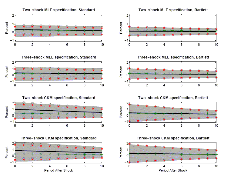
Data for Figure 5: Long-run Identification Results (percent)
| Period After Shock | Two-Shock MLE specification, Standard: Response: TRUE | Two-Shock MLE specification, Standard: Response: Estimated | Two-Shock MLE specification, Standard: Sampling Distribution: Lower Bound | Two-Shock MLE specification, Standard:Sampling Distribution: Upper Bound | Two-Shock MLE specification, Standard: Average CI Standard Deviation Based: Lower Bound | Two-Shock MLE specification, Standard: Average CI Standard Deviation Based: Upper Bound | Two-Shock MLE specification, Standard: Average CI Percentile Based: Lower Bound | Two-Shock MLE specification, Standard: Average CI Percentile Based: Upper Bound | Two-shock MLE specification, Bartlett: Response: TRUE | Two-shock MLE specification, Bartlett: Response: Estimated | Two-shock MLE specification, Bartlett: Sampling Distribution: Lower Bound | Two-shock MLE specification, Bartlett: Sampling Distribution: Upper Bound | Two-shock MLE specification, Bartlett: Average CI Standard Deviation Based: Lower Bound | Two-shock MLE specification, Bartlett: Average CI Standard Deviation Based: Upper Bound | Two-shock MLE specification, Bartlett: Average CI Percentile Based: Lower Bound | Two-shock MLE specification, Bartlett: Average CI Percentile Based: Upper Bound |
|---|---|---|---|---|---|---|---|---|---|---|---|---|---|---|---|---|
| 0 | 0.231057 | 0.289676 | -0.56289 | 0.810931 | -0.24935 | 0.828706 | -0.36018 | 0.65647 | 0.231057 | 0.105155 | -0.48134 | 0.632083 | -0.43523 | 0.645539 | -0.42096 | 0.633054 |
| 1 | 0.221202 | 0.281535 | -0.54349 | 0.804135 | -0.2481 | 0.811174 | -0.35252 | 0.651572 | 0.221202 | 0.100249 | -0.46359 | 0.60489 | -0.41372 | 0.614216 | -0.3997 | 0.60453 |
| 2 | 0.211766 | 0.271501 | -0.52456 | 0.800842 | -0.24725 | 0.790255 | -0.34876 | 0.639333 | 0.211766 | 0.095507 | -0.42724 | 0.585615 | -0.39252 | 0.583536 | -0.37927 | 0.576247 |
| 3 | 0.202734 | 0.262708 | -0.54301 | 0.799717 | -0.24628 | 0.771695 | -0.34153 | 0.630416 | 0.202734 | 0.092642 | -0.42826 | 0.564985 | -0.3716 | 0.556884 | -0.35959 | 0.551648 |
| 4 | 0.194086 | 0.249743 | -0.52404 | 0.775162 | -0.25133 | 0.750821 | -0.3414 | 0.615344 | 0.194086 | 0.085304 | -0.41533 | 0.543163 | -0.35536 | 0.525964 | -0.34106 | 0.519757 |
| 5 | 0.185808 | 0.239338 | -0.50002 | 0.762952 | -0.23762 | 0.716298 | -0.32426 | 0.590341 | 0.185808 | 0.081458 | -0.39563 | 0.517728 | -0.32766 | 0.490577 | -0.31405 | 0.48332 |
| 6 | 0.177883 | 0.230296 | -0.48517 | 0.741558 | -0.22866 | 0.689257 | -0.3112 | 0.571273 | 0.177883 | 0.077931 | -0.37354 | 0.492491 | -0.30705 | 0.462909 | -0.29344 | 0.45667 |
| 7 | 0.170295 | 0.220451 | -0.47291 | 0.727716 | -0.21755 | 0.658456 | -0.29606 | 0.548969 | 0.170295 | 0.074566 | -0.36034 | 0.470608 | -0.2838 | 0.432935 | -0.27098 | 0.427365 |
| 8 | 0.163032 | 0.210401 | -0.45182 | 0.717407 | -0.20899 | 0.629787 | -0.28339 | 0.527136 | 0.163032 | 0.070735 | -0.33841 | 0.453983 | -0.26434 | 0.405814 | -0.25275 | 0.400616 |
| 9 | 0.156078 | 0.201652 | -0.4373 | 0.700829 | -0.19994 | 0.603249 | -0.27079 | 0.507401 | 0.156078 | 0.06781 | -0.31753 | 0.443913 | -0.24569 | 0.38131 | -0.23473 | 0.376393 |
| 10 | 0.14942 | 0.193404 | -0.41767 | 0.689355 | -0.19247 | 0.57928 | -0.2598 | 0.489705 | 0.14942 | 0.065028 | -0.30679 | 0.425891 | -0.2296 | 0.359658 | -0.21978 | 0.35503 |
| Period After Shock | Three-Shock MLE specification, Standard: Response: TRUE | Three-Shock MLE specification, Standard: Response: Estimated | Three-Shock MLE specification, Standard: Sampling Distribution: Lower Bound | Three-Shock MLE specification, Standard:Sampling Distribution: Upper Bound | Three-Shock MLE specification, Standard: Average CI Standard Deviation Based: Lower Bound | Three-Shock MLE specification, Standard: Average CI Standard Deviation Based: Upper Bound | Three-Shock MLE specification, Standard: Average CI Percentile Based: Lower Bound | Three-Shock MLE specification, Standard: Average CI Percentile Based: Upper Bound | Three-shock MLE specification, Bartlett: Response: TRUE | Three-shock MLE specification, Bartlett: Response: Estimated | Three-shock MLE specification, Bartlett: Sampling Distribution: Lower Bound | Three-shock MLE specification, Bartlett: Sampling Distribution: Upper Bound | Three-shock MLE specification, Bartlett: Average CI Standard Deviation Based: Lower Bound | Three-shock MLE specification, Bartlett: Average CI Standard Deviation Based: Upper Bound | Three-shock MLE specification, Bartlett: Average CI Percentile Based: Lower Bound | Three-shock MLE specification, Bartlett: Average CI Percentile Based: Upper Bound |
|---|---|---|---|---|---|---|---|---|---|---|---|---|---|---|---|---|
| 0 | 0.227968 | 0.321596 | -0.94455 | 1.177234 | -0.52003 | 1.163218 | -0.62267 | 0.953856 | 0.227968 | 0.171726 | -0.65892 | 0.998247 | -0.69831 | 1.041767 | -0.66269 | 1.039794 |
| 1 | 0.218245 | 0.30471 | -0.93827 | 1.205732 | -0.53238 | 1.141802 | -0.62544 | 0.950611 | 0.218245 | 0.162159 | -0.65379 | 0.971568 | -0.65786 | 0.982179 | -0.62595 | 0.976519 |
| 2 | 0.208936 | 0.288413 | -0.94373 | 1.169734 | -0.53548 | 1.11231 | -0.62259 | 0.936964 | 0.208936 | 0.150499 | -0.65214 | 0.929636 | -0.6225 | 0.9235 | -0.59274 | 0.919375 |
| 3 | 0.200024 | 0.282122 | -0.92895 | 1.187192 | -0.52843 | 1.092675 | -0.61174 | 0.927821 | 0.200024 | 0.145215 | -0.62126 | 0.892868 | -0.58637 | 0.876797 | -0.55756 | 0.874256 |
| 4 | 0.191492 | 0.271278 | -0.90445 | 1.175605 | -0.52425 | 1.066803 | -0.60779 | 0.904703 | 0.191492 | 0.13654 | -0.58727 | 0.850243 | -0.56055 | 0.833629 | -0.5337 | 0.828337 |
| 5 | 0.183324 | 0.255028 | -0.87923 | 1.160452 | -0.50895 | 1.019009 | -0.58744 | 0.866951 | 0.183324 | 0.128196 | -0.55787 | 0.800487 | -0.52537 | 0.781759 | -0.4988 | 0.77528 |
| 6 | 0.175505 | 0.242805 | -0.8703 | 1.147439 | -0.5012 | 0.986812 | -0.57542 | 0.844939 | 0.175505 | 0.121769 | -0.5323 | 0.768648 | -0.50253 | 0.746066 | -0.47486 | 0.740424 |
| 7 | 0.168019 | 0.230056 | -0.8571 | 1.118676 | -0.49071 | 0.950822 | -0.56084 | 0.817033 | 0.168019 | 0.115281 | -0.51396 | 0.735898 | -0.47683 | 0.707392 | -0.44928 | 0.702422 |
| 8 | 0.160852 | 0.217086 | -0.84291 | 1.107298 | -0.48596 | 0.920136 | -0.5517 | 0.793303 | 0.160852 | 0.108222 | -0.48765 | 0.706562 | -0.45791 | 0.674356 | -0.43089 | 0.669156 |
| 9 | 0.153991 | 0.206461 | -0.83631 | 1.07805 | -0.47837 | 0.891297 | -0.53947 | 0.773561 | 0.153991 | 0.102808 | -0.46985 | 0.684111 | -0.43875 | 0.644366 | -0.41228 | 0.640125 |
| 10 | 0.147423 | 0.196914 | -0.81458 | 1.07255 | -0.47234 | 0.866163 | -0.52921 | 0.757129 | 0.147423 | 0.097773 | -0.45007 | 0.666064 | -0.4229 | 0.618448 | -0.3978 | 0.616195 |
| Period After Shock | Two-Shock CKM specification, Standard: Response: TRUE | Two-Shock CKM specification, Standard: Response: Estimated | Two-Shock CKM specification, Standard: Sampling Distribution: Lower Bound | CKM-Shock MLE specification, Standard:Sampling Distribution: Upper Bound | Two-Shock CKM specification, Standard: Average CI Standard Deviation Based: Lower Bound | Two-Shock CKM specification, Standard: Average CI Standard Deviation Based: Upper Bound | Two-Shock CKM specification, Standard: Average CI Percentile Based: Lower Bound | Two-Shock CKM specification, Standard: Average CI Percentile Based: Upper Bound | Two-shock CKM specification, Bartlett: Response: TRUE | Two-shock CKM specification, Bartlett: Response: Estimated | Two-shock CKM specification, Bartlett: Sampling Distribution: Lower Bound | Two-shock CKM specification, Bartlett: Sampling Distribution: Upper Bound | Two-shock CKM specification, Bartlett: Average CI Standard Deviation Based: Lower Bound | Two-shock CKM specification, Bartlett: Average CI Standard Deviation Based: Upper Bound | Two-shock CKM specification, Bartlett: Average CI Percentile Based: Lower Bound | Two-shock CKM specification, Bartlett: Average CI Percentile Based: Upper Bound |
|---|---|---|---|---|---|---|---|---|---|---|---|---|---|---|---|---|
| 0 | 0.317261 | 0.965227 | -0.5737 | 2.041564 | -0.23723 | 2.167689 | -0.54776 | 1.754532 | 0.317261 | 0.401947 | -1.06463 | 1.77546 | -0.95284 | 1.756733 | -0.95562 | 1.734179 |
| 1 | 0.303728 | 0.914762 | -0.5517 | 2.052182 | -0.24142 | 2.07094 | -0.52804 | 1.698675 | 0.303728 | 0.37738 | -0.99964 | 1.659215 | -0.87072 | 1.625484 | -0.869 | 1.611061 |
| 2 | 0.290773 | 0.862236 | -0.58651 | 1.896666 | -0.25437 | 1.978844 | -0.51244 | 1.641089 | 0.290773 | 0.358631 | -0.89623 | 1.56193 | -0.79641 | 1.51367 | -0.8029 | 1.501026 |
| 3 | 0.27837 | 0.813542 | -0.62769 | 1.83466 | -0.2612 | 1.888288 | -0.49405 | 1.584659 | 0.27837 | 0.336563 | -0.84174 | 1.445324 | -0.7307 | 1.40383 | -0.73075 | 1.402262 |
| 4 | 0.266497 | 0.757098 | -0.57787 | 1.773265 | -0.26403 | 1.778225 | -0.48408 | 1.497654 | 0.266497 | 0.313335 | -0.80083 | 1.3124 | -0.65894 | 1.285612 | -0.66792 | 1.275868 |
| 5 | 0.25513 | 0.696839 | -0.5213 | 1.695599 | -0.2468 | 1.640481 | -0.44142 | 1.390243 | 0.25513 | 0.287873 | -0.71307 | 1.212097 | -0.57857 | 1.15432 | -0.58406 | 1.144804 |
| 6 | 0.244248 | 0.646706 | -0.49512 | 1.605174 | -0.23834 | 1.531754 | -0.40723 | 1.309435 | 0.244248 | 0.266012 | -0.67691 | 1.118517 | -0.52158 | 1.053608 | -0.52553 | 1.046025 |
| 7 | 0.23383 | 0.59587 | -0.4539 | 1.560015 | -0.22609 | 1.417834 | -0.37322 | 1.222341 | 0.23383 | 0.244787 | -0.59762 | 1.040434 | -0.46167 | 0.95125 | -0.4631 | 0.945924 |
| 8 | 0.223856 | 0.547017 | -0.42835 | 1.49176 | -0.22499 | 1.319028 | -0.3532 | 1.143076 | 0.223856 | 0.223118 | -0.55751 | 0.9644 | -0.41996 | 0.866198 | -0.42055 | 0.862044 |
| 9 | 0.214308 | 0.505281 | -0.38415 | 1.418986 | -0.21635 | 1.226913 | -0.32337 | 1.073589 | 0.214308 | 0.205925 | -0.50252 | 0.902687 | -0.37653 | 0.78838 | -0.37433 | 0.789189 |
| 10 | 0.205167 | 0.467497 | -0.35197 | 1.361024 | -0.21042 | 1.145417 | -0.29882 | 1.010757 | 0.205167 | 0.190531 | -0.46913 | 0.863785 | -0.34116 | 0.722227 | -0.33682 | 0.727048 |
| Period After Shock | Three-Shock CKM specification, Standard: Response: TRUE | Three-Shock CKM specification, Standard: Response: Estimated | Three-Shock CKM specification, Standard: Sampling Distribution: Lower Bound | Three-Shock CKM specification, Standard:Sampling Distribution: Upper Bound | Three-Shock CKM specification, Standard: Average CI Standard Deviation Based: Lower Bound | Three-Shock CKM specification, Standard: Average CI Standard Deviation Based: Upper Bound | Three-Shock CKM specification, Standard: Average CI Percentile Based: Lower Bound | Three-Shock CKM specification, Standard: Average CI Percentile Based: Upper Bound | Three-shock CKM specification, Bartlett: Response: TRUE | Three-shock CKM specification, Bartlett: Response: Estimated | Three-shock CKM specification, Bartlett: Sampling Distribution: Lower Bound | Three-shock CKM specification, Bartlett: Sampling Distribution: Upper Bound | Three-shock CKM specification, Bartlett: Average CI Standard Deviation Based: Lower Bound | Three-shock CKM specification, Bartlett: Average CI Standard Deviation Based: Upper Bound | Three-shock CKM specification, Bartlett: Average CI Percentile Based: Lower Bound | Three-shock CKM specification, Bartlett: Average CI Percentile Based: Upper Bound |
|---|---|---|---|---|---|---|---|---|---|---|---|---|---|---|---|---|
| 0 | 0.317261 | 0.851112 | -0.90259 | 2.127806 | -0.40053 | 2.102756 | -0.63095 | 1.76735 | 0.317261 | 0.404461 | -1.16389 | 1.837508 | -1.07281 | 1.881728 | -1.03476 | 1.897182 |
| 1 | 0.303728 | 0.801645 | -0.87738 | 2.109122 | -0.39827 | 2.001562 | -0.60661 | 1.703234 | 0.303728 | 0.37956 | -1.05439 | 1.701848 | -0.95791 | 1.717034 | -0.9304 | 1.72348 |
| 2 | 0.290773 | 0.770071 | -0.84958 | 2.07164 | -0.38991 | 1.930049 | -0.58181 | 1.651805 | 0.290773 | 0.365329 | -0.94598 | 1.572458 | -0.86518 | 1.595842 | -0.84098 | 1.603683 |
| 3 | 0.27837 | 0.731267 | -0.78884 | 2.009485 | -0.39109 | 1.853628 | -0.56648 | 1.598786 | 0.27837 | 0.342985 | -0.91632 | 1.513652 | -0.7957 | 1.481667 | -0.77472 | 1.493743 |
| 4 | 0.266497 | 0.693385 | -0.72295 | 1.92564 | -0.36666 | 1.75343 | -0.5314 | 1.516108 | 0.266497 | 0.326585 | -0.86883 | 1.439891 | -0.71703 | 1.370203 | -0.70772 | 1.375656 |
| 5 | 0.25513 | 0.656799 | -0.60293 | 1.815994 | -0.32063 | 1.634232 | -0.46767 | 1.422802 | 0.25513 | 0.311235 | -0.75075 | 1.322529 | -0.62412 | 1.246591 | -0.61411 | 1.249644 |
| 6 | 0.244248 | 0.625136 | -0.57637 | 1.733189 | -0.29391 | 1.544177 | -0.41964 | 1.357026 | 0.244248 | 0.298135 | -0.65295 | 1.288795 | -0.56011 | 1.156377 | -0.54712 | 1.163023 |
| 7 | 0.23383 | 0.591828 | -0.50264 | 1.651405 | -0.27084 | 1.454497 | -0.38222 | 1.287398 | 0.23383 | 0.283388 | -0.60395 | 1.223977 | -0.49973 | 1.066505 | -0.48668 | 1.075609 |
| 8 | 0.223856 | 0.559127 | -0.43887 | 1.572853 | -0.26133 | 1.379589 | -0.35995 | 1.22807 | 0.223856 | 0.268636 | -0.53633 | 1.156231 | -0.4575 | 0.994768 | -0.44405 | 1.002715 |
| 9 | 0.214308 | 0.530744 | -0.41011 | 1.471036 | -0.2494 | 1.310886 | -0.33421 | 1.174993 | 0.214308 | 0.256049 | -0.48587 | 1.082434 | -0.41687 | 0.928965 | -0.40242 | 0.938054 |
| 10 | 0.205167 | 0.504108 | -0.38807 | 1.404788 | -0.24266 | 1.250874 | -0.31447 | 1.130154 | 0.205167 | 0.244043 | -0.4462 | 1.036987 | -0.3856 | 0.873685 | -0.36862 | 0.885256 |
Figure 6: Analyzing Precision in Inference
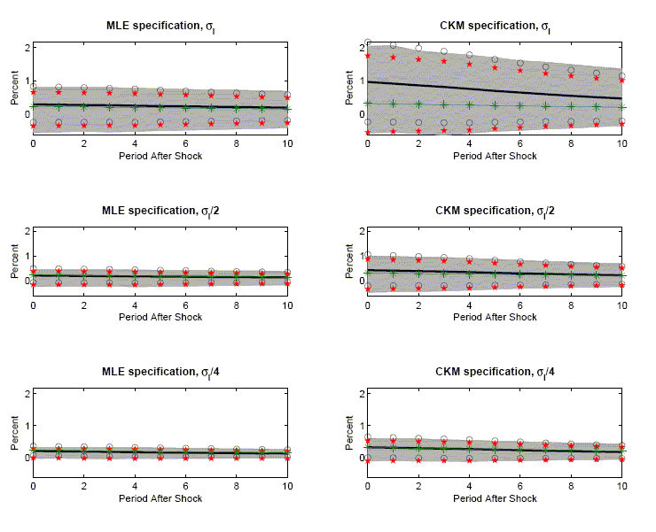
Data for Figure 6: Analyzing Precision in Inference (percent)
| Period After Shock | MLE specification, |
MLE specification, |
MLE specification, |
MLE specification, |
MLE specification, |
MLE specification, |
MLE specification, |
MLE specification, |
CKM specification, |
CKM specification, |
CKM specification, |
CKM specification, |
CKM specification, |
CKM specification, |
CKM specification, |
CKM specification, |
|---|---|---|---|---|---|---|---|---|---|---|---|---|---|---|---|---|
| 0 | 0.231057 | 0.289676 | -0.56289 | 0.810931 | -0.24935 | 0.828706 | -0.36018 | 0.65647 | 0.317261 | 0.965227 | -0.5737 | 2.041564 | -0.23723 | 2.167689 | -0.54776 | 1.754532 |
| 1 | 0.221202 | 0.281535 | -0.54349 | 0.804135 | -0.2481 | 0.811174 | -0.35252 | 0.651572 | 0.303728 | 0.914762 | -0.5517 | 2.052182 | -0.24142 | 2.07094 | -0.52804 | 1.698675 |
| 2 | 0.211766 | 0.271501 | -0.52456 | 0.800842 | -0.24725 | 0.790255 | -0.34876 | 0.639333 | 0.290773 | 0.862236 | -0.58651 | 1.896666 | -0.25437 | 1.978844 | -0.51244 | 1.641089 |
| 3 | 0.202734 | 0.262708 | -0.54301 | 0.799717 | -0.24628 | 0.771695 | -0.34153 | 0.630416 | 0.27837 | 0.813542 | -0.62769 | 1.83466 | -0.2612 | 1.888288 | -0.49405 | 1.584659 |
| 4 | 0.194086 | 0.249743 | -0.52404 | 0.775162 | -0.25133 | 0.750821 | -0.3414 | 0.615344 | 0.266497 | 0.757098 | -0.57787 | 1.773265 | -0.26403 | 1.778225 | -0.48408 | 1.497654 |
| 5 | 0.185808 | 0.239338 | -0.50002 | 0.762952 | -0.23762 | 0.716298 | -0.32426 | 0.590341 | 0.25513 | 0.696839 | -0.5213 | 1.695599 | -0.2468 | 1.640481 | -0.44142 | 1.390243 |
| 6 | 0.177883 | 0.230296 | -0.48517 | 0.741558 | -0.22866 | 0.689257 | -0.3112 | 0.571273 | 0.244248 | 0.646706 | -0.49512 | 1.605174 | -0.23834 | 1.531754 | -0.40723 | 1.309435 |
| 7 | 0.170295 | 0.220451 | -0.47291 | 0.727716 | -0.21755 | 0.658456 | -0.29606 | 0.548969 | 0.23383 | 0.59587 | -0.4539 | 1.560015 | -0.22609 | 1.417834 | -0.37322 | 1.222341 |
| 8 | 0.163032 | 0.210401 | -0.45182 | 0.717407 | -0.20899 | 0.629787 | -0.28339 | 0.527136 | 0.223856 | 0.547017 | -0.42835 | 1.49176 | -0.22499 | 1.319028 | -0.3532 | 1.143076 |
| 9 | 0.156078 | 0.201652 | -0.4373 | 0.700829 | -0.19994 | 0.603249 | -0.27079 | 0.507401 | 0.214308 | 0.505281 | -0.38415 | 1.418986 | -0.21635 | 1.226913 | -0.32337 | 1.073589 |
| 10 | 0.14942 | 0.193404 | -0.41767 | 0.689355 | -0.19247 | 0.57928 | -0.2598 | 0.489705 | 0.205167 | 0.467497 | -0.35197 | 1.361024 | -0.21042 | 1.145417 | -0.29882 | 1.010757 |
| Period After Shock | MLE specification, |
MLE specification, |
MLE specification, |
MLE specification, |
MLE specification, |
MLE specification, |
MLE specification, |
MLE specification, |
CKM specification, |
CKM specification, |
CKM specification, |
CKM specification, |
CKM specification, |
CKM specification, |
CKM specification, |
CKM specification, |
|---|---|---|---|---|---|---|---|---|---|---|---|---|---|---|---|---|
| 0 | 0.231057 | 0.210906 | -0.23928 | 0.44873 | -0.07263 | 0.494439 | -0.1528 | 0.38436 | 0.317261 | 0.426006 | -0.4685 | 1.00459 | -0.20548 | 1.057492 | -0.33593 | 0.869008 |
| 1 | 0.221202 | 0.20237 | -0.22924 | 0.441947 | -0.0769 | 0.48164 | -0.1519 | 0.380285 | 0.303728 | 0.406312 | -0.44723 | 0.981755 | -0.19992 | 1.012548 | -0.3219 | 0.841089 |
| 2 | 0.211766 | 0.192385 | -0.22934 | 0.439963 | -0.0832 | 0.467969 | -0.15361 | 0.373439 | 0.290773 | 0.388226 | -0.43328 | 0.952395 | -0.19792 | 0.974369 | -0.30987 | 0.817935 |
| 3 | 0.202734 | 0.182589 | -0.22297 | 0.445458 | -0.08847 | 0.453648 | -0.15611 | 0.364797 | 0.27837 | 0.37193 | -0.41554 | 0.940841 | -0.194 | 0.937861 | -0.29692 | 0.795577 |
| 4 | 0.194086 | 0.175374 | -0.2445 | 0.436871 | -0.09073 | 0.441477 | -0.1544 | 0.357013 | 0.266497 | 0.348006 | -0.38115 | 0.908067 | -0.19679 | 0.892798 | -0.29209 | 0.759203 |
| 5 | 0.185808 | 0.167271 | -0.2316 | 0.42552 | -0.08582 | 0.420367 | -0.14623 | 0.341343 | 0.25513 | 0.320667 | -0.3409 | 0.869498 | -0.18249 | 0.823825 | -0.26749 | 0.705256 |
| 6 | 0.177883 | 0.160808 | -0.21755 | 0.412886 | -0.0825 | 0.404112 | -0.13921 | 0.329518 | 0.244248 | 0.298194 | -0.3103 | 0.822821 | -0.17264 | 0.769026 | -0.2467 | 0.664448 |
| 7 | 0.170295 | 0.153599 | -0.20534 | 0.403814 | -0.07836 | 0.385556 | -0.13158 | 0.315702 | 0.23383 | 0.275265 | -0.2935 | 0.779299 | -0.16176 | 0.712288 | -0.22655 | 0.619661 |
| 8 | 0.163032 | 0.147148 | -0.19547 | 0.397502 | -0.07454 | 0.36883 | -0.12436 | 0.303493 | 0.223856 | 0.253617 | -0.27301 | 0.753587 | -0.15391 | 0.661145 | -0.21043 | 0.579449 |
| 9 | 0.156078 | 0.14063 | -0.18522 | 0.394737 | -0.07166 | 0.352918 | -0.11861 | 0.291455 | 0.214308 | 0.234932 | -0.2597 | 0.715045 | -0.14539 | 0.615257 | -0.19282 | 0.543699 |
| 10 | 0.14942 | 0.134519 | -0.17494 | 0.387264 | -0.06939 | 0.338426 | -0.11354 | 0.280469 | 0.205167 | 0.217668 | -0.23863 | 0.690665 | -0.13917 | 0.574505 | -0.17854 | 0.512139 |
| Period After Shock | MLE specification, |
MLE specification, |
MLE specification, |
MLE specification, |
MLE specification, |
MLE specification, |
MLE specification, |
MLE specification, |
CKM specification, |
CKM specification, |
CKM specification, |
CKM specification, |
CKM specification, |
CKM specification, |
CKM specification, |
CKM specification, |
|---|---|---|---|---|---|---|---|---|---|---|---|---|---|---|---|---|
| 0 | 0.231057 | 0.202356 | -0.03268 | 0.307991 | 0.052635 | 0.352076 | -0.00977 | 0.276081 | 0.317261 | 0.318734 | -0.1179 | 0.602859 | -0.00947 | 0.646935 | -0.10575 | 0.522908 |
| 1 | 0.221202 | 0.192648 | -0.02878 | 0.313275 | 0.042578 | 0.342717 | -0.01603 | 0.273672 | 0.303728 | 0.305368 | -0.10075 | 0.588801 | -0.01315 | 0.623883 | -0.10211 | 0.512215 |
| 2 | 0.211766 | 0.183896 | -0.03732 | 0.319046 | 0.032986 | 0.334805 | -0.02203 | 0.270267 | 0.290773 | 0.289948 | -0.11947 | 0.585012 | -0.01929 | 0.59919 | -0.09995 | 0.497898 |
| 3 | 0.202734 | 0.174894 | -0.04674 | 0.313968 | 0.024074 | 0.325714 | -0.02728 | 0.26557 | 0.27837 | 0.277487 | -0.12012 | 0.558601 | -0.02454 | 0.579511 | -0.09921 | 0.486508 |
| 4 | 0.194086 | 0.165596 | -0.0332 | 0.307502 | 0.017589 | 0.313602 | -0.02964 | 0.257551 | 0.266497 | 0.262405 | -0.12845 | 0.53979 | -0.03048 | 0.555293 | -0.09789 | 0.468251 |
| 5 | 0.185808 | 0.156648 | -0.0404 | 0.300271 | 0.01484 | 0.298456 | -0.02919 | 0.245466 | 0.25513 | 0.244072 | -0.11009 | 0.513599 | -0.02919 | 0.517338 | -0.09023 | 0.437761 |
| 6 | 0.177883 | 0.149376 | -0.03609 | 0.293449 | 0.012269 | 0.286482 | -0.02828 | 0.236537 | 0.244248 | 0.227821 | -0.11109 | 0.494903 | -0.02993 | 0.485572 | -0.08368 | 0.413597 |
| 7 | 0.170295 | 0.141602 | -0.03059 | 0.277448 | 0.009863 | 0.273341 | -0.02776 | 0.225762 | 0.23383 | 0.211666 | -0.08877 | 0.473493 | -0.02984 | 0.453171 | -0.07687 | 0.388479 |
| 8 | 0.163032 | 0.135085 | -0.02771 | 0.272083 | 0.008232 | 0.261938 | -0.02592 | 0.217155 | 0.223856 | 0.197013 | -0.07723 | 0.454074 | -0.02999 | 0.42402 | -0.07049 | 0.366278 |
| 9 | 0.156078 | 0.128097 | -0.02637 | 0.265127 | 0.00592 | 0.250275 | -0.02567 | 0.207617 | 0.214308 | 0.182936 | -0.07005 | 0.439053 | -0.03116 | 0.397028 | -0.06591 | 0.344898 |
| 10 | 0.14942 | 0.121609 | -0.0245 | 0.259728 | 0.003647 | 0.239571 | -0.02523 | 0.199064 | 0.205167 | 0.170125 | -0.06049 | 0.417588 | -0.03271 | 0.37296 | -0.06197 | 0.326313 |
Figure 7: Varying the Labor Elasticity in the Two-shock CKM Specification
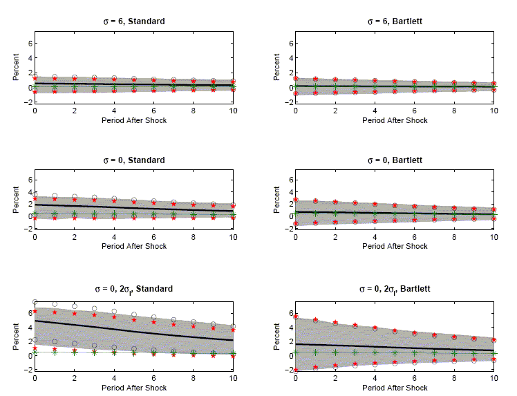
Data for Figure 7: Varying the Labor Elasticity in the Two-shock CKM specification (percent)
|
Period After Shock |
|
|||||||||||||||
|---|---|---|---|---|---|---|---|---|---|---|---|---|---|---|---|---|
| 0 | 0.122083 | 0.530941 | -0.76794 | 1.454371 | -0.43084 | 1.492717 | -0.61339 | 1.220703 | 0.122083 | 0.168674 | -1.03915 | 1.274497 | -0.86488 | 1.202232 | -0.82025 | 1.223388 |
| 1 | 0.117775 | 0.507677 | -0.78177 | 1.411787 | -0.42204 | 1.437398 | -0.5918 | 1.187444 | 0.117775 | 0.160606 | -0.97209 | 1.193033 | -0.80239 | 1.123596 | -0.75818 | 1.147591 |
| 2 | 0.113618 | 0.487617 | -0.70523 | 1.395412 | -0.41134 | 1.386573 | -0.56543 | 1.15754 | 0.113618 | 0.1554 | -0.92088 | 1.101551 | -0.74323 | 1.05403 | -0.70118 | 1.080689 |
| 3 | 0.109609 | 0.464566 | -0.72735 | 1.347642 | -0.40532 | 1.334449 | -0.54673 | 1.124306 | 0.109609 | 0.14859 | -0.88088 | 1.041175 | -0.69222 | 0.9894 | -0.65537 | 1.014775 |
| 4 | 0.105741 | 0.433406 | -0.67353 | 1.277555 | -0.40311 | 1.269926 | -0.53894 | 1.071706 | 0.105741 | 0.13693 | -0.83113 | 0.964751 | -0.64105 | 0.914911 | -0.60919 | 0.930973 |
| 5 | 0.102009 | 0.404719 | -0.59728 | 1.22969 | -0.37146 | 1.180896 | -0.4933 | 1.003061 | 0.102009 | 0.128985 | -0.73438 | 0.915514 | -0.57157 | 0.829534 | -0.54275 | 0.844298 |
| 6 | 0.09841 | 0.380428 | -0.56737 | 1.181033 | -0.34841 | 1.109261 | -0.45832 | 0.950038 | 0.09841 | 0.122118 | -0.66284 | 0.863069 | -0.51845 | 0.762689 | -0.49313 | 0.776887 |
| 7 | 0.094937 | 0.354807 | -0.52225 | 1.12587 | -0.3241 | 1.033715 | -0.42299 | 0.891757 | 0.094937 | 0.114538 | -0.617 | 0.788495 | -0.46479 | 0.693863 | -0.44325 | 0.708376 |
| 8 | 0.091586 | 0.328211 | -0.4816 | 1.08809 | -0.30878 | 0.965202 | -0.39868 | 0.83684 | 0.091586 | 0.105248 | -0.56279 | 0.737689 | -0.42369 | 0.634185 | -0.40502 | 0.647067 |
| 9 | 0.088354 | 0.30685 | -0.4523 | 1.04743 | -0.28906 | 0.902758 | -0.36788 | 0.788929 | 0.088354 | 0.099128 | -0.52149 | 0.693609 | -0.38266 | 0.580915 | -0.36563 | 0.595468 |
| 10 | 0.085236 | 0.287438 | -0.42084 | 1.004767 | -0.27299 | 0.84787 | -0.34214 | 0.74673 | 0.085236 | 0.093473 | -0.49107 | 0.660393 | -0.3485 | 0.535443 | -0.33308 | 0.551339 |
|
Period After Shock |
|
|||||||||||||||
|---|---|---|---|---|---|---|---|---|---|---|---|---|---|---|---|---|
| 0 | 0.475978 | 1.886516 | -0.36851 | 3.219048 | 0.230943 | 3.542089 | -0.31862 | 2.8741 | 0.475978 | 0.713306 | -1.59699 | 2.57335 | -1.26399 | 2.690598 | -1.19064 | 2.739748 |
| 1 | 0.452677 | 1.778356 | -0.50613 | 3.146697 | 0.174209 | 3.382503 | -0.32836 | 2.786861 | 0.452677 | 0.67716 | -1.36983 | 2.483957 | -1.13299 | 2.48731 | -1.06844 | 2.532761 |
| 2 | 0.430518 | 1.681075 | -0.27372 | 3.098105 | 0.121613 | 3.240538 | -0.33032 | 2.701988 | 0.430518 | 0.641294 | -1.29145 | 2.414946 | -1.02863 | 2.31122 | -0.95812 | 2.359559 |
| 3 | 0.409443 | 1.586166 | -0.45737 | 2.980229 | 0.067145 | 3.105187 | -0.33912 | 2.613931 | 0.409443 | 0.613208 | -1.21342 | 2.2316 | -0.93201 | 2.158423 | -0.86542 | 2.2152 |
| 4 | 0.389399 | 1.457312 | -0.40756 | 2.862199 | 0.009759 | 2.904865 | -0.35874 | 2.460654 | 0.389399 | 0.557095 | -1.11997 | 2.12092 | -0.84944 | 1.963631 | -0.79024 | 2.0132 |
| 5 | 0.370337 | 1.329944 | -0.33519 | 2.695049 | -0.02083 | 2.680721 | -0.34272 | 2.28272 | 0.370337 | 0.50662 | -1.00843 | 1.994265 | -0.74546 | 1.758701 | -0.69285 | 1.797438 |
| 6 | 0.352208 | 1.22469 | -0.30175 | 2.510417 | -0.04916 | 2.498538 | -0.32285 | 2.143125 | 0.352208 | 0.466244 | -0.92188 | 1.842566 | -0.66617 | 1.598654 | -0.61022 | 1.637799 |
| 7 | 0.334967 | 1.118379 | -0.24402 | 2.376348 | -0.07401 | 2.310766 | -0.30481 | 1.991026 | 0.334967 | 0.425467 | -0.8204 | 1.703178 | -0.58852 | 1.439451 | -0.53472 | 1.473908 |
| 8 | 0.318569 | 1.021517 | -0.21816 | 2.261767 | -0.10753 | 2.150562 | -0.29953 | 1.864883 | 0.318569 | 0.385281 | -0.74664 | 1.596839 | -0.53877 | 1.309335 | -0.48632 | 1.342865 |
| 9 | 0.302974 | 0.93353 | -0.19285 | 2.138047 | -0.1271 | 1.994159 | -0.28001 | 1.74181 | 0.302974 | 0.352355 | -0.67026 | 1.506221 | -0.48207 | 1.186781 | -0.42832 | 1.224433 |
| 10 | 0.288143 | 0.854252 | -0.17209 | 2.033628 | -0.14542 | 1.85392 | -0.2636 | 1.633743 | 0.288143 | 0.322297 | -0.58746 | 1.382422 | -0.43701 | 1.081603 | -0.38097 | 1.123652 |
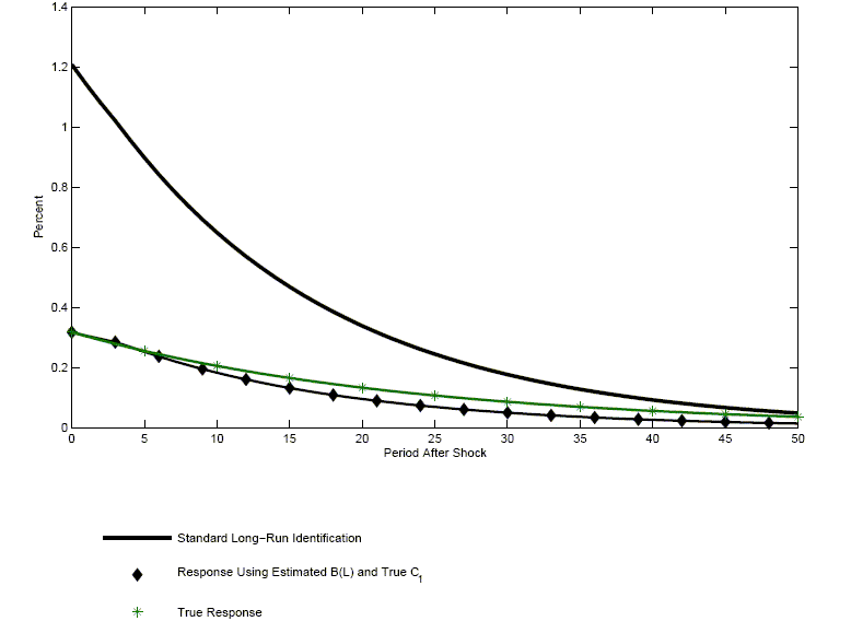
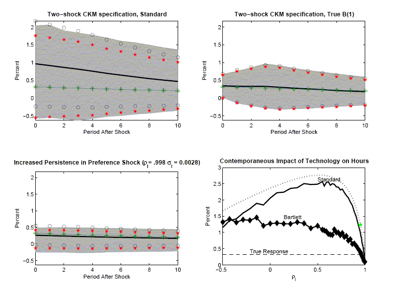
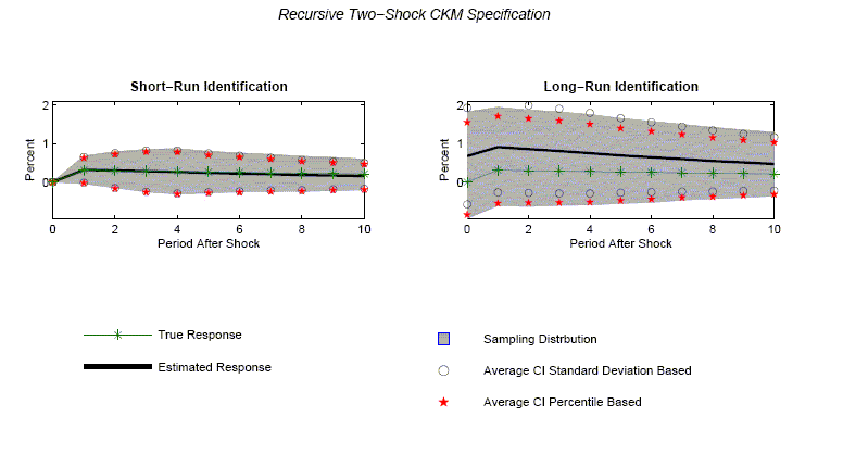
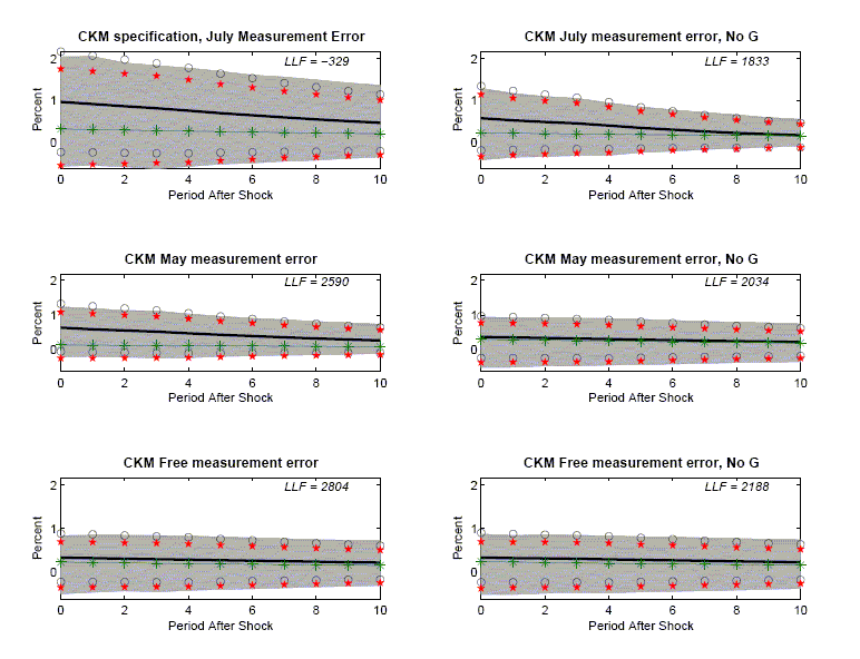
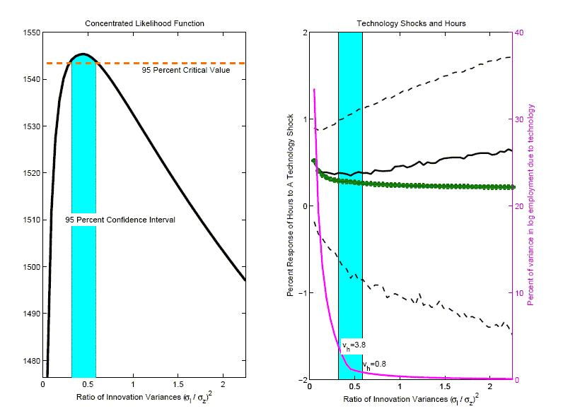
![\begin{displaymath}B_{1}=\left[ \begin{array}[c]{cc} 0.013 & 0.041\ 0.0065 & 0.94 \end{array}\right] ,\end{displaymath}](img1tab2.gif)
![\begin{displaymath}B_{2}=\left[ \begin{array}[c]{cc} 0.012 & -0.00\ 0.0062 & -0.00 \end{array}\right] ,\end{displaymath}](img2tab2.gif)
![\begin{displaymath}B_{3}=\left[ \begin{array}[c]{cc} 0.012 & -0.00\ 0.0059 & -0.00 \end{array}\right] ,\end{displaymath}](img3tab2.gif)
![\begin{displaymath}B_{4}=\left[ \begin{array}[c]{cc} 0.011 & -0.00\ 0.0056 & -0.00 \end{array}\right] ,\end{displaymath}](img4tab2.gif)
![\begin{displaymath}B_{5}=\left[ \begin{array}[c]{cc} 0.011 & -0.00\ 0.0054 & -0.00 \end{array}\right] ,\end{displaymath}](img5tab2.gif)
![\begin{displaymath}B_{6}=\left[ \begin{array}[c]{cc} 0.010 & -0.00\ 0.0051 & -0.00 \end{array}\right] \end{displaymath}](img6tab2.gif)
![\begin{displaymath}\hat{B}_{1}=\left[ \begin{array}[c]{cc} 0.017 & 0.043\ 0.0087 & 0.94 \end{array}\right] ,\end{displaymath}](img7tab2.gif)
![\begin{displaymath}\hat{B}_{2}=\left[ \begin{array}[c]{cc} 0.017 & -0.00\ 0.0085 & -0.00 \end{array}\right] ,\end{displaymath}](img8tab2.gif)
![\begin{displaymath}\hat{B}_{3}=\left[ \begin{array}[c]{cc} 0.012 & -0.00\ 0.0059 & -0.00 \end{array}\right] ,\end{displaymath}](img9tab2.gif)
![\begin{displaymath}\hat{B}_{4}=\left[ \begin{array}[c]{cc} 0.0048 & -0.0088\ 0.0025 & -0.0045 \end{array}\right] \end{displaymath}](img10tab2.gif)
![\begin{displaymath}\hat{B}\left( 1\right) =\left[ \begin{array}[c]{cc} 0.055 & 0... ...{array}[c]{cc} 0.28 & 0.022\ 0.14 & 0.93 \end{array}\right] ,\end{displaymath}](img11tab2.gif)
![\begin{displaymath}\sum_{j=1}^{4}B_{j}=\left[ \begin{array}[c]{cc} 0.047 & 0.039\ 0.024 & 0.94 \end{array}\right] \end{displaymath}](img12tab2.gif)
![\begin{displaymath}S_{Y}\left( 0\right) =\left[ \begin{array}[c]{cc} 0.00017 & 0.00097\ 0.00097 & 0.12 \end{array}\right] ,\end{displaymath}](img13tab2.gif)
![\begin{displaymath}\hat{S}_{Y}\left( 0\right) =\left[ \begin{array}[c]{cc} 0.00012 & 0.0022\ 0.0022 & 0.13 \end{array}\right] .\end{displaymath}](img14tab2.gif)
![\begin{displaymath}V=\hat{V}=\left[ \begin{array}[c]{cc} 0.00012 & -0.00015\ -0.00015 & -0.00053 \end{array}\right] \end{displaymath}](img15tab2.gif)
![\begin{displaymath}C_{1}=\left( \begin{array}[c]{c} 0.00773\ 0.00317 \end{array}\right) ,\end{displaymath}](img16tab2.gif)
![\begin{displaymath}\hat{C}_{1}=\left( \begin{array}[c]{c} 0.00406\ 0.01208 \end{array}\right) \end{displaymath}](img17tab2.gif)